Limited Feedback Channel Estimation in Massive MIMO with Non-uniform Directional Dictionaries

Abstract

Channel state information (CSI) at the base station (BS) is crucial to achieve beamforming and multiplexing gains in multiple-input multiple-output (MIMO) systems. State-of-the-art limited feedback schemes require feedback overhead that scales linearly with the number of BS antennas, which is prohibitive for $5$G massive MIMO. This work proposes novel limited feedback algorithms that lift this burden by exploiting the inherent sparsity in double directional (DD) MIMO channel representation using overcomplete dictionaries. These dictionaries are associated with angle of arrival (AoA) and angle of departure (AoD) that specifically account for antenna directivity patterns at both ends of the link. The proposed algorithms achieve satisfactory channel estimation accuracy using a small number of feedback bits, even when the number of transmit antennas at the BS is large – making them ideal for $5$G massive MIMO. Judicious simulations reveal that they outperform a number of popular feedback schemes, and underscore the importance of using angle dictionaries matching the given antenna directivity patterns, as opposed to uniform dictionaries. The proposed algorithms are lightweight in terms of computation, especially on the user equipment side, making them ideal for actual deployment in $5$G systems.

I Introduction

The idea of harnessing a large number of antennas at the base station (BS), possibly many more than the number of user equipment (UE) terminals in the cell, has recently attracted a lot of interest in massive multiple-input multiple-output (MIMO) research. The key technical reasons for this is that massive MIMO can enable leaps in spectral efficiency [1] as well as help mitigating intercell interference through simple linear precoding and combining, offering immunity to small-scale fading – known as the channel hardening effect [2, 3]. Massive MIMO systems also have the advantage of being energy-efficient since every antenna may operate at a low-energy level [4].

Acquiring accurate and timely downlink channel state information (CSI) at the BS is the key to realize the multiplexing and array gains enabled by MIMO systems [2, 5, 6, 7]. Acquiring accurate downlink CSI at the BS using only few feedback bits from the UE is a major challenge, especially in massive MIMO systems. In frequency division duplex (FDD) systems, where channel reciprocity does not hold, the BS cannot acquire downlink channel information from uplink training sequences, and the feedback overhead may be required to scale proportionally to the number of BS antennas [5]. In time division duplex (TDD) systems, channel reciprocity between uplink and downlink is often assumed, and the BS acquires downlink CSI through uplink training. Even in TDD mode, however, relying only on channel reciprocity is not accurate enough, since the uplink measurements at the BS cannot capture the downlink interference from neighboring cells [8, 9]. Thus, downlink reference signals are still required to estimate and feed back the channel quality indicator (CQI), meaning that some level of feedback is practically necessary for both FDD and TDD modes.

The largest portion of the feedback-based channel estimation literature explores various quantization techniques; see [10] for a well-rounded exposition. Many of these methods utilize a vector quantization (VQ) codebook that is known to both the BS and the UE. After estimating the instantaneous downlink CSI at the UE, the UE sends through a limited feedback channel the index of the codeword that best matches the estimated channel, in the sense of minimizing the outage probability [11], maximizing link capacity [12], or maximizing the beamforming gain [13, 14]. Codebooks for spatially correlated channels based on generalizations of the Lloyd algorithm are given in [15], while codebooks designed for temporally correlated channels are provided in [16]. Codebook-free feedback for channel tracking was considered in [17] for spatio-temporally correlated channels with imperfect CSI at the UE. Many limited feedback approaches in MIMO systems consider a Rayleigh fading channel model [18, 13, 14, 19]. Under this channel model, the number of VQ feedback bits required to guarantee reasonable performance is linear in the number of transmit antennas at the BS [5] – which is costly in the case of massive MIMO. Yet the designer is not limited to using VQ-based approaches, and massive MIMO channels can be far from Rayleigh.

In this work, we consider an approach that differs quite sharply from the prevailing limited feedback methodologies. Our approach specifically targets FDD massive MIMO in the sublinear feedback regime. We adopt the double directional (DD) MIMO channel model [20] (see also [21]) instead of the Rayleigh fading model. The DD channel model parameterizes each channel path using angle of departure (AoD) at BS, small- and large-scale propagation coefficients, and angle of arrival (AoA) at UE – a parametrization that is well-accepted and advocated by 3GPP [22, 23]. We exploit a ‘virtual sparse representation’ of the downlink channel under the double directional MIMO model [20]. Quantizing AoA and AoD, it is possible to design overcomplete dictionaries that contain steering vectors approximating those associated with the true angles of arrival and departure. Building upon [20], such representation has been exploited to design receiver-side millimeter wave (mmWave) channel estimation algorithms using high-resolution [24], or low-resolution (coarsely quantized) analog-to-digital converters (ADCs) [25, 26].

In contrast, we focus on transmitter-side (BS) downlink channel acquisition using only limited receiver-side (UE) computation and feedback to the BS [27]. We propose novel optimization formulations and algorithms for downlink channel estimation at the BS using single-bit judiciously-compressed measurements. In this way, we shift the channel computation burden from the UE to the BS, while keeping the feedback overhead low. Using the overcomplete parametrization of the DD model, three new limited feedback setups are proposed:

• In the first setup, UE applies dictionary-based sparse channel estimation and support identification to estimate the 2D angular support and the corresponding coefficients of the sparse channel. Then, the UE feeds back the support of the sparse channel estimate, plus a coarsely quantized version of the corresponding non-zero coefficients, assuming known thresholds at the BS. This is the proposed UE-based limited feedback baseline method for the DD model.

• In the second setup, the UE compresses the received measurements and sends back only the signs of the compressed measurements to the BS. Upon receiving these sign bits, the BS estimates the channel using single-bit DD dictionary-based sparse estimation algorithms.

• The third setup is a combination of the first and the second, called hybrid limited feedback: UE estimates and sends the support of the sparse channel estimate on top of the compressed sign feedback used in the second setup. Upon receiving this augmented feedback from the UE, the BS can then apply the algorithms of setup 2 on a significantly reduced problem dimension.

For sparse estimation and support identification, the orthogonal matching pursuit (OMP) algorithm [28] is utilized as it offers the best possible computational complexity among all sparse estimation algorithms [29], which is highly desired for resource-constrained UE terminals.

Contributions:

A new limited feedback channel estimation framework is proposed exploiting the sparse nature of the DD model (setup 2). Two formulations are proposed based on single-bit sparse maximum-likelihood estimation (MLE) and single-bit compressed sensing. For MLE, an optimal in terms of iteration complexity [30] first-order proximal method is designed using adaptive restart, to further speed up the convergence rate [31]. The proposed compressed sensing (CS) formulation can be – fortuitously – harnessed by invoking the recent single-bit CS literature. The underlying convex optimization problem has a simple closed-form solution, which is ideal for practical implementation. The proposed framework shifts the computational burden towards the BS side – the UE only carries out matrix-vector multiplications and takes signs. This is sharply different from most limited feedback schemes in the literature, where the UE does the ‘heavy lifting’ [6, 10]. More importantly, under our design, using a small number of feedback bits achieves very satisfactory channel estimation accuracy even when the number of BS antennas is very large, as long as the number of paths is reasonably small – which is usually the case in practice [20]; thus, the proposed framework is ideal for massive MIMO 5G cellular networks.

In addition to the above contributions, a new angle dictionary construction methodology is proposed to enhance performance, based on a companding quantization technique [32]. The idea is to create dictionaries that concentrate the angle density in a non-uniform manner, around the angles where directivity patterns attain higher values. The baseline 3GPP antenna directivity pattern is considered for this, and the end-to-end results are contrasted with those obtained using uniform quantization, to showcase this important point. Judicious simulations reveal that the proposed dictionaries outperform uniform dictionaries.

Last but not least, to further reduce computational complexity at the BS and enhance beamforming and ergodic rate performance, a new hybrid implementation is proposed (setup 3). This setup is very effective when the UE is capable of carrying out simple estimation algorithms, such as OMP. At the relatively small cost of communicating extra support information that slightly increases feedback communication overhead, the BS applies the single-bit MLE and single-bit CS algorithms on a dramatically reduced problem dimension. Simulations reveal that the performance of the two algorithms under setup 3 is always better than under setup 2. As in setup 2, the feedback overhead is tightly controlled by the system designer and the desired level of channel estimation accuracy is attained with very small feedback rate, even in the massive MIMO regime.

Comprehensive simulations over a range of pragmatic scenarios, based on the 3GPP DD channel model [33], compare the proposed methods with baseline least-squares (LS) scalar and vector quantization (VQ) feedback strategies in terms of normalized mean-squared estimation error (NRMSE), beamforming gain, and multi-user capacity under zero-forcing (ZF) beamforming. Unlike VQ, which requires that the number of feedback bits grows at least linearly with the number of BS antennas to maintain a certain level of estimation performance, the number of feedback bits of the proposed algorithms is controlled by the system designer, and substantial feedback overhead reduction is observed for achieving better performance compared to VQ methods. It is also shown that when the sparse DD model is valid, the proposed methods not only outperform LS schemes, but they may also offer performance very close to perfect CSI in some cases.

Relative to the conference precursor [34] of this work, this journal version includes the following additional contributions: the UE-based limited feedback scheme under setup 1; the novel channel estimation algorithm based on the sparse MLE formulation; the new hybrid schemes under setup 3; and comprehensive (vs. illustrative) simulations of all schemes considered. The rest of this paper is organized as follows. Section II presents the adopted wireless system model, and Section III derives the proposed non-uniform directional dictionaries. Sections IV, V, and VI develop the proposed UE-based, BS-based, and hybrid limited feedback algorithms, respectively. Section VII presents simulation results, and Section VIII summarizes conclusions.

Notation: Boldface lowercase and uppercase letters denote column vectors and matrices, respectively; $()^{*}$, $()^{\top}$, and $()^{\mathsf{H}}$, denote conjugate, transpose, and Hermitian operators, respectively. $\|\cdot\|_{p}$, $\Re(\cdot)$, $\Im(\cdot)$, and $|\cdot|$ denote the $p$-norm (with $p\in[0,\infty]$), the real, the imaginary, and the absolute or set cardinality operator, respectively. $\mathsf{diag}(\mathbf{x})$ is the diagonal matrix formed by vector $\mathbf{x}$, $\mathbf{0}$ is the all-zero vector and its size is understood from the context, $\mathbf{I}_{N}$ is the $N\times N$ identity matrix. Symbol $\otimes$ denotes the Kronecker product. $\mathbb{E}[\cdot]$ is the expectation operator. $\mathcal{CN}(\boldsymbol{\mu},\boldsymbol{\Sigma})$ denotes the proper complex Gaussian distribution with mean $\boldsymbol{\mu}$ and covariance $\boldsymbol{\Sigma}$. Matrix (vector) $\mathbf{A}_{:,\mathcal{S}}$ ($\mathbf{x}_{\mathcal{S}}$) comprises of the columns of matrix $\mathbf{A}$ (elements of $\mathbf{x}$) indexed by set $\mathcal{S}$. Function $\mathsf{sign}(x)=1$ for $x\geq 0$ and zero, otherwise; abusing notation a bit, we also apply it to vectors, element-wise. Function $(x)_{+}=\max(0,x)$, $\mathsf{j}\triangleq\sqrt{-1}$ is the imaginary unit, and $\mathsf{Q}(x)=\frac{1}{\sqrt{2\pi}}\int_{x}^{\infty}\mathsf{e}^{-t^{2}/2}\mathsf{d}t$ is the $\mathsf{Q}$-function.

II System Model

We consider an FDD cellular system consisting of a BS serving $K$ active UE terminals, where the downlink channel is estimated at the BS through feedback from each UE. For brevity of exposition, we focus on a single UE. The proposed algorithms can be easily generalized to multiple users, as the downlink channel estimation process can be performed separately for each UE. The BS is equipped with $M_{\rm T}$ antennas and the UE is equipped with $M_{\rm R}$ antennas. The channel is assumed static over a coherence block of $U_{\rm c}=B_{\rm c}T_{\rm c}(\frac{T_{\rm s}-T_{\rm g}}{T_{\rm s}})$ complex orthogonal frequency division multiplexing (OFDM) symbols, where $B_{\rm c}$ is the coherence bandwidth (in Hz), $T_{\rm c}$ is the coherence time (in seconds), and quantity $(\frac{T_{\rm s}-T_{\rm g}}{T_{\rm s}})$ indicates the fraction of useful symbol time (i.e., $T_{\rm s}$ is the OFDM symbol duration and $T_{\rm g}$ is the cyclic prefix duration). In downlink transmission, the BS has to acquire CSI through feedback from the active UE terminals, and then design the transmit signals accordingly. At the training phase, the BS employs $N_{\rm tr}$ training symbols for channel estimation. The narrowband (over time-frequency) discrete model over a period of $N_{\rm tr}$ training symbols is given by

$$\mathbf{y}_{n}=\mathbf{H}\,\mathbf{s}_{n}+\mathbf{n}_{n},~{}~{}n=1,2,\ldots,N_{\rm tr},$$ (1)

where $n$ is the $n$-th training index, $\mathbf{s}_{n}\in\mathds{C}^{M_{\rm T}}$ is the transmitted training signal, $\mathbf{y}_{n}\in\mathds{C}^{M_{\rm R}}$ is the received vector, $\mathbf{H}\in\mathds{C}^{M_{\rm R}\times M_{\rm T}}$ denotes the complex baseband equivalent channel matrix, and $\mathbf{n}_{n}\sim\mathcal{CN}(\mathbf{0},\sigma^{2}\mathbf{I}_{M_{\rm R}})$ is additive Gaussian noise at the receiver of variance $\sigma^{2}$. All quantities in the right hand-side of (1) are independent of each other; $\mathbb{E}[\mathbf{s}_{n}\mathbf{s}_{n}^{\mathsf{H}}]=\frac{P_{\rm T}}{M_{\rm T}}\mathbf{I}_{M_{\rm T}}$, for all $n$, where $P_{\rm T}$ denotes the average total transmit power. The signal-to-noise ratio (SNR) is defined as ${\rm SNR}\triangleq\frac{P_{\rm T}}{\sigma^{2}}$.

To estimate $\mathbf{H}$, we can use linear least-squares (LS) [18], or, if the channel covariance is known, the linear minimum mean-squared error (LMMSE) approach [6]. These linear approaches need more than $M_{\rm T}M_{\rm R}$ training symbols to establish identifiability of the channel (to ‘over-determine’ the problem) – which is rather costly in massive MIMO scenarios.

A more practical approach to the problem of downlink channel acquisition at the BS of massive MIMO systems would be to shift the computational burden to the BS, relying on relatively lightweight computations at the UE, and assuming that only low-rate feedback is available as well. The motivation for this is clear: the BS is connected to the communication backbone, plugged to the power grid, and may even have access to cloud computing – thus is far more capable of performing intensive computations. The challenge of course is how to control the feedback overhead – without a limitation on feedback rate, the UE can of course simply relay the signals that receives back to the BS, but such an approach is clearly wasteful and impractical. The ultimate goal is to achieve accurate channel estimation with low feedback overhead, i.e., estimate $\mathbf{H}$ using just a few feedback bits.

Towards this end, our starting idea is to employ a finite scatterer (also known as discrete multipath, or double directional) channel model comprising of $L$ paths, which can be parameterized using a virtual sparse representation. The inherent sparsity of DD parameterization in the angle-delay domain can be exploited also at the the UE side to estimate the downlink channel using compressed sensing techniques with reduced pilot sequence overhead [20]. This sparse representation will lead to a feedback scheme that is rather parsimonious in terms of both overhead and computational complexity. The narrowband downlink channel matrix $\mathbf{H}$ can be written as

$$\mathbf{H}\!=\!\sqrt{\frac{M_{\rm T}M_{\rm R}}{L}}\sum_{l=1}^{L}\alpha_{l}\,\mathsf{c}_{\rm T}(\phi_{l}^{\prime})\,\mathsf{c}_{\rm R}(\phi_{l})\,\mathbf{a}_{\rm R}(\phi_{l})\,\mathbf{a}_{{\rm T}}^{\mathsf{H}}(\phi_{l}^{\prime})\,\mathsf{e}^{\mathsf{j}\varphi_{l}},$$ (2)

where $\alpha_{l}$ is the complex gain of the $l$-th path incorporating path-losses, small- and large-scale fading effects; variables $\phi_{l}$ and $\phi_{l}^{\prime}$ are the azimuth angle of arrival (AoA) and angle of departure (AoD) for the $l$th path, respectively; and $\mathbf{a}_{\rm T}(\cdot)\in\mathds{C}^{M_{\rm T}}$, $\mathbf{a}_{\rm R}(\cdot)\in\mathds{C}^{M_{\rm R}}$ represent the transmit and receive array steering vectors, respectively, which depend on the antenna array geometry. Random phase $\varphi_{l}$ is associated with the delay of the $l$-th path. Functions $\mathsf{c}_{\rm T}(\cdot)$ and $\mathsf{c}_{\rm R}(\cdot)$ represent the BS and UE antenna element directivity pattern, respectively (all transmit antenna elements are assumed to have the same directivity pattern, and the same holds for the receive antenna elements). Examples of transmit and receive antenna patterns are the uniform directivity pattern over a sector $[\phi_{\rm T}^{\rm l},\phi_{\rm T}^{\rm u}]$, given by $\mathsf{c}_{\rm T}(\phi)=1$, when $\phi\in[\phi_{\rm T}^{\rm l},\phi_{\rm T}^{\rm u}]$ and $\mathsf{c}_{\rm T}(\phi)=0$, otherwise, and likewise for $\mathsf{c}_{\rm R}(\phi)$. Another baseline directivity pattern is advocated by 3GPP [36]

$$\mathsf{c}_{\rm T}(\phi)=10^{\frac{\mathtt{G}_{\rm dB}}{20}+\max\left\{-0.6\left(\frac{\phi}{\phi_{\rm 3dB}}\right)^{2},-\frac{\mathtt{A}_{m}}{20}\right\}},$$ (3)

with $\phi\in[-\pi,\pi)$, where $\mathtt{G}_{\rm dB}$ is the maximum directional gain of the radiation element in dBi, $\mathtt{A}_{m}$ is the front-to-back ratio in dB, and $\phi_{\rm 3dB}$ is the $3$dB-beamwidth. A common antenna array architecture is the uniform linear array (ULA) (w.r.t. $y$ axis) using only the azimuth angle; in this case the BS steering vector (similarly for UE) is given by

$$\mathbf{a}_{\rm T}(\phi)=\sqrt{\frac{1}{{M_{\rm T}}}}\left[1~{}\mathsf{e}^{-\mathsf{j}\frac{2\pi d_{y}}{\lambda}\mathsf{sin}(\phi)}~{}\ldots~{}\mathsf{e}^{-\mathsf{j}\frac{2\pi d_{y}(M_{\rm T}-1)}{\lambda}\mathsf{sin}(\phi)}\right]^{\top},$$ (4)

where $\lambda$ is the carrier wavelength, and $d_{y}$ is the distance between the antenna elements along the $y$ axis (usually $d_{y}=\lambda/2$).

The channel in (2) can be written more compactly as

$$\mathbf{H}=\mathbf{A}_{\rm R}\mathsf{diag}(\boldsymbol{\alpha})\mathbf{A}_{\rm T}^{\mathsf{H}},$$ (5)

with matrices $\mathbf{A}_{\rm R}\triangleq[\mathsf{c}_{\rm R}(\phi_{1})\mathbf{a}_{\rm R}(\phi_{1})~{}\ldots~{}\mathsf{c}_{\rm R}(\phi_{L})\mathbf{a}_{\rm R}(\phi_{L})]$ and $\mathbf{A}_{\rm T}\triangleq[\mathsf{c}_{\rm T}(\phi_{1}^{\prime})\mathbf{a}_{\rm T}(\phi_{1}^{\prime})~{}\ldots~{}\mathsf{c}_{\rm T}(\phi_{L}^{\prime})\mathbf{a}_{\rm T}(\phi_{L}^{\prime})]$ denoting all transmit and receive steering vectors in compact form, respectively, while vector $\boldsymbol{\alpha}\triangleq\sqrt{\frac{M_{\rm T}M_{\rm R}}{L}}[\alpha_{1}\mathsf{e}^{\mathsf{j}\varphi_{1}}~{}\ldots~{}\alpha_{L}\mathsf{e}^{\mathsf{j}\varphi_{L}}]^{\top}$ collects the path-loss and phase shift coefficients. Starting from the model in (5), one can come up with a sparse representation of the channel [20]. First, the angle space of AoA and AoD is quantized by discretizing the angular space. Let us denote these dictionaries $\mathcal{P}_{\rm T}$ and $\mathcal{P}_{\rm R}$ for AoDs and AoAs, respectively. Dictionary $\mathcal{P}_{\rm T}$ contains $G_{\rm T}$ dictionary members, while $\mathcal{P}_{\rm R}$ contains $G_{\rm R}$ dictionary members. One simple way of constructing these dictionaries is to use a uniform grid of phases in an angular sector $\left[a,b\right)\subseteq[-\pi,\pi)$. In that case, $\mathcal{P}_{\rm R}=\left\{a+\frac{j\,(b-a)}{G_{\rm R}+1}\right\}_{j=1}^{G_{\rm R}}$ and $\mathcal{P}_{\rm T}=\left\{a+\frac{j\,(b-a)}{G_{\rm T}+1}\right\}_{j=1}^{G_{\rm T}}$. For given dictionaries $\mathcal{P}_{\rm R}$ and $\mathcal{P}_{\rm T}$, dictionary matrices are defined

$$\widetilde{\mathbf{A}}_{\rm R}\triangleq ~{}\{\mathsf{c}_{\rm R}(\phi)\,\mathbf{a}_{\rm R}(\phi):\phi\in\mathcal{P}_{\rm R}\}\in\mathds{C}^{M_{\rm R}\times{G}_{\rm R}},$$ (6)

$$\widetilde{\mathbf{A}}_{\rm T}\triangleq ~{}\{\mathsf{c}_{\rm T}(\phi)\,\mathbf{a}_{\rm T}(\phi):\phi\in\mathcal{P}_{\rm T}\}\in\mathds{C}^{M_{\rm T}\times{G}_{\rm T}},$$ (7)

which stand for an overcomplete quantized approximation of the matrices $\mathbf{A}_{\rm R}$ and $\mathbf{A}_{\rm T}$, respectively. Hence, the channel matrix in the left-hand side of (5) can be written, up to some quantization errors, as

$$\mathbf{H}\approx\widetilde{\mathbf{A}}_{\rm R}\mathbf{G}\widetilde{\mathbf{A}}_{\rm T}^{\mathsf{H}},$$ (8)

where matrix $\mathbf{G}\in\mathds{C}^{{G}_{\rm R}\times{G}_{\rm T}}$ is an interaction matrix, whose $(j,k)$th element is associated with the $j$th and $k$th columns in $\widetilde{\mathbf{A}}_{\rm R}$ and $\widetilde{\mathbf{A}}_{\rm T}$, respectively – if $[{\bf G}]_{j,k}\neq 0$, this means that a propagation path associated with the $k$th angle in ${\cal P}_{\rm T}$ and the $j$th angle in ${\cal P}_{\rm R}$ is active. In practice, the number of active paths is typically very small compared to the number of elements of $\mathbf{G}$ (i.e., $G_{\rm T}G_{\rm R}$). Thus, the matrix $\mathbf{G}$ is in most cases very sparse [20].

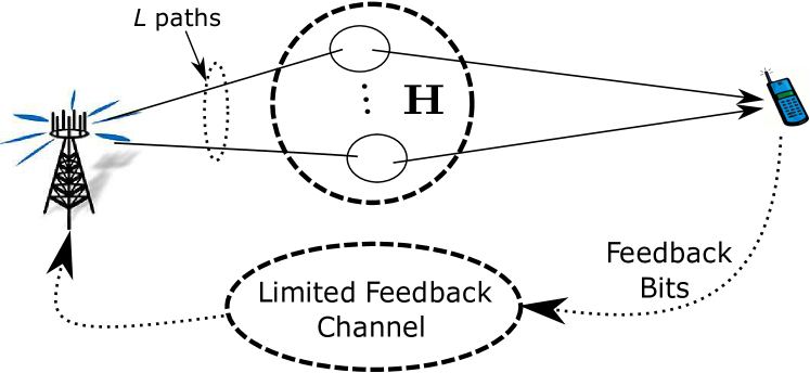
Figure 1: System model: UE receives $\mathbf{y}$, employs one of the three limited feedback setups to compress the downlink channel matrix $\mathbf{H}$, feeds back the bits to the BS through a limited feedback channel, and the BS reconstructs $\mathbf{H}$.

Stacking all columns $\{\mathbf{y}_{n}\}_{n=1}^{N_{\rm tr}}$ in (1) in a parallel fashion, we form matrix $\mathbf{Y}=[\mathbf{y}_{1}~{}\mathbf{y}_{2}~{}\ldots~{}\mathbf{y}_{N_{\rm tr}}]$. Denoting $\mathbf{S}=[\mathbf{s}_{1}~{}\mathbf{s}_{2}~{}\ldots~{}\mathbf{s}_{N_{\rm tr}}]$ for the transmitted training symbol sequence and $\mathbf{N}=[\mathbf{n}_{1}~{}\mathbf{n}_{2}~{}\ldots~{}\mathbf{n}_{N_{\rm tr}}]$ for the noise, and using the channel matrix approximation in (8), the baseband signal in (1) can be written in a compact matrix form as

$$\mathbf{Y}=\widetilde{\mathbf{A}}_{\rm R}\mathbf{G}\widetilde{\mathbf{A}}_{\rm T}^{\mathsf{H}}\mathbf{S}+\mathbf{N}.$$ (9)

Applying the vectorization property $\mathsf{vec}(\mathbf{ABC})=(\mathbf{C}^{\top}\otimes\mathbf{A})\mathsf{vec}(\mathbf{B})$ in Eq. (9), the baseband received signal is given by

$$\mathbf{y}=\left((\mathbf{S}^{\top}\widetilde{\mathbf{A}}_{\rm T}^{*})\otimes\widetilde{\mathbf{A}}_{\rm R}\right)\mathbf{g}+\mathbf{n}=\mathbf{Q}\mathbf{g}+\mathbf{n},$$ (10)

where $\mathbf{y}\triangleq\mathsf{vec}(\mathbf{Y})\in\mathds{C}^{{M_{\rm R}N_{\rm tr}}}$, $\mathbf{g}\triangleq\mathsf{vec}(\mathbf{G})\in\mathds{C}^{G_{\rm T}G_{\rm R}}$, $\mathbf{n}\triangleq\mathsf{vec}(\mathbf{N})\in\mathds{C}^{{M_{\rm R}N_{\rm tr}}}$, and $\mathbf{Q}\triangleq(\mathbf{S}^{\top}\widetilde{\mathbf{A}}_{\rm T}^{*})\otimes\widetilde{\mathbf{A}}_{\rm R}\in\mathds{C}^{{M_{\rm R}N_{\rm tr}}\times G_{\rm T}G_{\rm R}}$. We define $G\triangleq G_{\rm T}G_{\rm R}$ the joint (product) dictionary size. This quantity plays a pivotal role on the performance of the algorithms considered, since it determines the angle granularity of the dictionaries, which in turn determines the ultimate estimation error performance. Fig. 1 provides a high-level overview of the system model.

III Angle Dictionary Construction Accounting for Antenna Directivity Patterns

Before introducing the proposed feedback schemes, let us consider the practical issue of quantizing the angular space. Prior art on channel estimation employs the sparse representation in (5) using uniformly discretized angles as dictionaries [20]. However, a more appealing angle dictionary should take into consideration the antenna directivity patterns, since the channel itself naturally reflects the directivity pattern. In this work we propose the following: pack more angles around the peaks of the antenna directivity pattern, because the dominant paths will likely fall in those regions, and this is where we need higher angular resolution. Denser discretization within high-antenna-power regions can reduce quantization errors more effectively compared to a uniform quantization that ignores the directivity pattern.

To explain our approach, let $\mathsf{q}:[a,b)\longrightarrow\mathds{R}^{+}$ be a given antenna directivity pattern function, which is assumed continuous over $\phi\in[a,b)$ and suppose that we want to represent it using $N$ quantization points; see Fig. 2 for the 3GPP directivity pattern. We define the cumulative function of $\mathsf{q}$, given by $\mathsf{G}(\phi)\triangleq\int_{a}^{\phi}\mathsf{q}(x)\mathsf{d}x$. As the range space of function $\mathsf{q}$ takes positive values, its continuity implies that $\mathsf{G}$ is monotone increasing. Thus, the following set

$$\mathcal{C}_{\mathsf{q}}\triangleq\left\{\mathsf{G}(a)+\frac{n(\mathsf{G}(b)-\mathsf{G}(a))}{N+1},\right\}_{n=1}^{N},$$ (11)

partitions the range of $\mathsf{G}$ in $N+1$ intervals of equal size. By the definition of $\mathsf{G}$, the set in (11) partitions function $\mathsf{q}$ in $N+1$ equal area intervals. Having the elements of set $\mathcal{C}_{\mathsf{q}}$, we can find the phases at which $\mathsf{q}(\phi)$ is partitioned in $N+1$ equal area intervals – which means that we achieve our goal of putting denser grids in the angular region where the ${\sf q}$ function has higher intensity. These phases can be found as

$$\mathcal{F}_{\mathsf{q}}\triangleq\left\{\mathsf{G}^{-1}(y)\right\}_{y\in\mathcal{C}_{\mathsf{q}}},$$ (12)

where $\mathsf{G}^{-1}:[\mathsf{G}(a),\mathsf{G}(b))\longrightarrow[a,b)$ is the inverse (with respect to composition) function of $\mathsf{G}$. Observe that $\mathsf{G}^{-1}$ is a continuous, monotone increasing function since $\mathsf{G}$ is itself continuous and monotone increasing. The discrete set $\mathcal{F}_{\mathsf{q}}$ is a subset of $[a,b)$ and concentrates more elements at points where function $\mathsf{q}$ has larger values.

Let us exemplify the procedure of constructing the angle dictionaries using the 3GPP antenna directivity pattern. As the most general case [36], we assume $a\leq-\phi_{\rm 3dB}\sqrt{\frac{\mathtt{A}_{\rm m}}{12}}$ and $b\geq\phi_{\rm 3dB}\sqrt{\frac{\mathtt{A}_{\rm m}}{12}}$. The domain of $\mathsf{q}$ can be partitioned into 3 disjoint intervals as $[a,b)=[a,-\phi_{0})\cup[-\phi_{0},\phi_{0})\cup[\phi_{0},b)$, with $\phi_{0}\triangleq\phi_{\rm 3dB}\sqrt{\frac{\mathtt{A}_{\rm m}}{12}}$. Using $\mathsf{q}(x)\equiv\mathsf{c}_{\rm T}(x)$ in Eq. (3), applying the definition of cumulative function $\mathsf{G}(\phi)=\int_{a}^{\phi}\mathsf{q}(x)\mathsf{d}x$, and using its continuity, we obtain [34]

$$\mathsf{G}(\phi)\!=\!\begin{cases}(\phi-a)10^{\frac{\mathtt{G}_{\rm dB}}{20}-\frac{\mathtt{A}_{m}}{20}},&\!\phi\in[a,-\phi_{0}),\\ \mathsf{G}\!\left(-\phi_{0}\right)+10^{\frac{\mathtt{G}_{\rm dB}}{20}}\sqrt{\frac{\pi\,\phi_{\rm 3dB}^{2}}{\mathsf{ln}(10)\,2.4}}\cdot&\\ \left(\mathsf{erf}\!\left(\sqrt{\frac{\mathsf{ln}(10)\,0.6\,\mathtt{A}_{m}}{12}}\right)+\right.&\\ \left.\mathsf{sign}(\phi)\mathsf{erf}\!\left(\sqrt{\frac{\mathsf{ln}(10)\,0.6}{\phi_{\rm 3dB}^{2}}}|\phi|\right)\right),&\!\phi\in[-\phi_{0},\phi_{0}),\\ \mathsf{G}\!\left(\phi_{0}\right)+\left(\phi-\phi_{0}\right)10^{\frac{\mathtt{G}_{\rm dB}}{20}-\frac{\mathtt{A}_{m}}{20}},&\!\phi\in[\phi_{0},b),\end{cases}$$ (13)

where $\mathsf{erf}(x)\frac{\sqrt{\pi}}{2}=\int_{0}^{x}\mathsf{e}^{-t^{2}}\mathsf{d}t$ was utilized. Upon defining $y^{-}\triangleq\mathsf{G}(-\phi_{0})$, $y_{0}\triangleq\mathsf{G}(0)$, and $y^{+}\triangleq\mathsf{G}(\phi_{0})$, the inverse of $\mathsf{G}(\cdot)$ can be calculated using Eq. (13) in closed form as

$$\mathsf{G}^{-1}\!(y)\!=\!\begin{cases}y\,10^{\frac{\mathtt{A}_{m}}{20}-\frac{\mathtt{G}_{\rm dB}}{20}}+a,&\!y\in[0,y^{-}),\\ -\frac{\mathsf{erf}^{-1}\!\left(\frac{2\sqrt{\mathsf{ln}(10)\,0.6}}{\phi_{\rm 3dB}\sqrt{\pi}}(y_{0}-y)10^{-\frac{\mathtt{G}_{\rm dB}}{20}}\right)}{\frac{\sqrt{\mathsf{ln}(10)\,0.6}}{\phi_{\rm 3dB}}},&\!y\in[y^{-},y_{0}),\\ \frac{\mathsf{erf}^{-1}\!\left(\frac{2\sqrt{\mathsf{ln}(10)\,0.6}}{\phi_{\rm 3dB}\sqrt{\pi}}(y-y_{0})10^{-\frac{\mathtt{G}_{\rm dB}}{20}}\right)}{\frac{\sqrt{\mathsf{ln}(10)\,0.6}}{\phi_{\rm 3dB}}},&\!y\in[y_{0},y^{+}),\\ \phi_{0}+(y-y^{+})10^{\frac{\mathtt{A}_{m}}{20}-\frac{\mathtt{G}_{\rm dB}}{20}},&\!y\in[y^{+},\mathsf{G}(b)),\end{cases}$$ (14)

where $\mathsf{erf}^{-1}(\cdot)$ is the inverse (with respect to composition) function of $\mathsf{erf}(\cdot)$, and is well tabulated by several software packages, such as Matlab. The definition of inverse function in (14) for interval $[a,b)$, such that $[-\phi_{0},\phi_{0})\subseteq[a,b)\subseteq[-\pi,\pi)$, is the most general case. As one can see in Fig. 2, the point density of this quantization of the angular space indeed reflects the selectivity of the antenna directivity pattern, as desired.

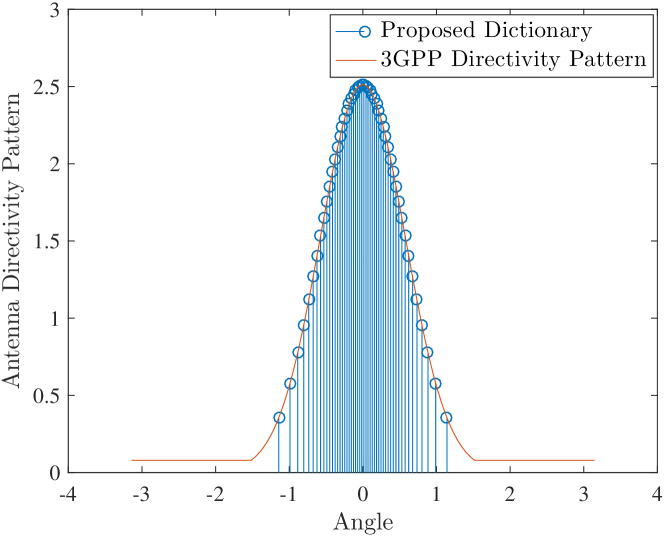
Figure 2: 3GPP directivity pattern along with function $\mathsf{q}$ applied on the proposed dictionary using $a=-\pi$ and $b=\pi$. The proposed angle dictionaries pack more points around higher values of $\mathsf{q}$.

IV UE-based Baseline Limited Feedback Sparse Channel Estimation

This section presents a baseline limited feedback setup where UE estimates the sparse channel and sends back the support along with the coarsely quantized nonzero elements of the estimated sparse channel $\mathbf{g}$.

IV-A Channel Estimation and Support Identification at UE

The inherent sparsity of $\mathbf{g}$ in (10) suggests the following formulation to recover it at UE

$$\min_{\mathbf{g}\in\mathds{C}^{G}:\|\mathbf{g}\|_{0}\leq L}\!\left\{\frac{1}{2}\|\mathbf{y}-\mathbf{Q}\mathbf{g}\|_{2}^{2}\right\}.$$ (15)

The optimization problem in (15) is a non-convex combinatorial problem. Prior art in compressed sensing (CS) optimization literature has attempted to solve (15) using approximation algorithms, such as orthogonal matching pursuit (OMP) [28], iterative hard thresholding (IHT) [37], and many others; see [29] and references therein. OMP-based algorithms are preferable for sparse channel estimation, due to their favorable performance-complexity trade-off [29]. OMP admits simple and even real-time implementation, and its run-time complexity can be further reduced by caching the QR factorization of matrix $\mathbf{Q}$ [28]. For completeness, the pseudo code for OMP is provided in Algorithm 1. For a detailed discussion regarding the implementation details and performance guarantees of the OMP algorithm the reader is referred to [38].

Algorithm 1 Channel Estimation and Support Identification at UE

Input: $\mathbf{Q},\mathbf{y}$, $\overline{L}$

1:$t=0:$ Initialize $\mathbf{r}=\mathbf{y}$, $\mathcal{S}_{\widehat{\mathbf{g}}}=\emptyset$

2:while $\|\mathbf{Q}^{\mathsf{H}}\mathbf{r}\|_{\infty}>\varepsilon$ and $t<\overline{L}$  do

3:    $t:=t+1$

4:    $\mathbf{p}=\mathbf{Q}^{\mathsf{H}}\mathbf{r}$

5:    $n^{\star}=\arg\max_{n=1,2,\ldots G}\{|p_{n}|\}$

6:    $\mathcal{S}_{\widehat{\mathbf{g}}}:=\mathcal{S}_{\widehat{\mathbf{g}}}\cup n^{\star}$

7:    $\widehat{\mathbf{g}}_{\mathcal{S}_{\widehat{\mathbf{g}}}^{\mathtt{C}}}=\mathbf{0}$ and $\widehat{\mathbf{g}}_{\mathcal{S}_{\widehat{\mathbf{g}}}}=\mathbf{Q}_{:,\mathcal{S}_{\widehat{\mathbf{g}}}}^{\dagger}\mathbf{y}$

8:    $\mathbf{r}=\mathbf{y}-\mathbf{Q}\,\widehat{\mathbf{g}}$

9:end while

Output: $\widehat{\mathbf{g}}$, $\mathcal{S}_{\widehat{\mathbf{g}}}$

IV-B Scalar Quantization and Limited Feedback

After estimating the sparse vector $\widehat{\mathbf{g}}$ associated with an estimate of interaction matrix $\widehat{\mathbf{G}}$ a simple feedback technique is to send coarsely quantized non-zero elements of $\widehat{\mathbf{g}}$, along with the corresponding indices. In this work we make use of Lloyd’s scalar quantizer to quantize the non-zero elements of $\widehat{\mathbf{g}}$, and we denote the scalar quantization operation $\mathsf{SQ}(\widehat{\mathbf{g}})$. Upon receiving the bits associated with the non-zero indices and elements of $\widehat{\mathbf{g}}$, i.e., $\mathcal{S}_{\widehat{\mathbf{g}}}$ and $\mathsf{SQ}(\widehat{\mathbf{g}})$, the BS reconstructs channel matrix $\widehat{\mathbf{H}}$ via (8), provided it has perfect knowledge of SQ threshold values. As the channel model in (10) has sparse structure comprising $L$ non-zero elements, for suitably designed $\mathbf{Q}$ and a sufficient number of training symbols, this approach tends to yield a channel estimate comprising $\mathcal{O}(L)$ non-zero elements.

Using a $Q$-bit real scalar quantizer, each non-zero element of complex vector $\widehat{\mathbf{g}}$ can be represented using $\lceil\mathsf{log}_{2}G\rceil+2Q$ bits, where the first term accounts for index coding, and the second for coding the real and imaginary parts. Hence, the total number of feedback bits to estimate the interaction matrix $\mathbf{G}$ at the BS, scales with $\mathcal{O}(L(\lceil\mathsf{log}_{2}G\rceil+2Q))$. In the worst case, OMP iterates $\overline{L}$ times, offering worst case feedback overhead $\overline{L}(\lceil\mathsf{log}_{2}G\rceil+2Q)$. Note that the number of feedback bits of the proposed UE-based baseline limited feedback algorithm is independent of $M_{\rm T}$.

V BS-based Limited Feedback Sparse Channel Estimation

In order to reduce the feedback overhead without irrevocably sacrificing our ability to recover accurate CSI at the BS, we propose to apply a pseudo-random dimensionality-reducing linear operator $\mathbf{P}^{\mathsf{H}}$ to $\mathbf{y}$. The outcome is quantized with a very simple sign quantizer, whose output is fed back to the BS through a low-rate channel. More precisely, the BS receives

$$\mathbf{b}_{\Re}+\mathsf{j}\,\mathbf{b}_{\Im}=\mathsf{sign}(\Re\!\left(\mathbf{P}^{\mathsf{H}}\mathbf{y}\right))+\mathsf{j}\,\mathsf{sign}\!\left(\Im\!\left(\mathbf{P}^{\mathsf{H}}\mathbf{y}\right)\right),$$ (16)

where $\mathbf{P}\in\mathds{C}^{M_{\rm R}N_{\rm tr}\times N_{\rm fb}}$, with $N_{\rm fb}\leq M_{\rm R}N_{\rm tr}$.

To facilitate operating in the more convenient real domain, consider the following definitions

$$\mathbf{C}_{\Re}^{\top} \triangleq\left[{\Re}(\mathbf{Q}^{\mathsf{H}}\mathbf{P})^{\top}~{}{\Im}(\mathbf{Q}^{\mathsf{H}}\mathbf{P})^{\top}\right],$$ (17a)

$$~{}~{}\mathbf{C}_{\Im}^{\top} \triangleq\left[-{\Im}(\mathbf{Q}^{\mathsf{H}}\mathbf{P})^{\top}~{}{\Re}(\mathbf{Q}^{\mathsf{H}}\mathbf{P})^{\top}\right],$$ (17b)

$${\mathbf{C}} \triangleq[\mathbf{C}_{\Re}~{}~{}\mathbf{C}_{\Im}]=\left[\mathbf{c}_{1}~{}\mathbf{c}_{2}\ldots~{}\mathbf{c}_{2N_{\rm fb}}\right]\in\mathds{R}^{2G\times 2N_{\rm fb}},$$ (17c)

$$\mathbf{x}^{\top} \triangleq\left[{\Re}(\mathbf{g})^{\top}~{}{\Im}(\mathbf{g})^{\top}\right]\in\mathds{R}^{2G},~{}~{}$$ (17d)

$$\mathbf{b}^{\top} \triangleq\left[\mathbf{b}_{\Re}^{\top}~{}\mathbf{b}_{\Im}^{\top}\right]^{\top}=[b_{1}~{}b_{2}~{}\ldots~{}b_{2N_{\rm fb}}]\in\mathds{R}^{2N_{\rm fb}},$$ (17e)

$$\mathbf{z}^{\top} \triangleq\left[\mathbf{z}_{\Re}^{\top}~{}\mathbf{z}_{\Im}^{\top}\right]^{\top}=[z_{1}~{}z_{2}~{}\ldots~{}z_{2N_{\rm fb}}]\in\mathds{R}^{2N_{\rm fb}},$$ (17f)

with $\Re\!\left(\mathbf{P}^{\mathsf{H}}\mathbf{Q}\mathbf{g}\right)=\mathbf{C}_{\Re}^{\top}\mathbf{x}$, $\Im\!\left(\mathbf{P}^{\mathsf{H}}\mathbf{Q}\mathbf{g}\right)=\mathbf{C}_{\Im}^{\top}\mathbf{x}$, $\mathbf{z}_{\Re}=\Re\!\left(\mathbf{P}^{\mathsf{H}}\mathbf{n}\right)$, and $\mathbf{z}_{\Im}=\Im\!\left(\mathbf{P}^{\mathsf{H}}\mathbf{n}\right)$. Using the above, along with (16), the received feedback bits at the BS are given by

$$b_{i}=\mathsf{sign}\!\left(\mathbf{c}_{i}^{\top}\mathbf{x}+z_{i}\right),~{}~{}i=1,2,\ldots,2N_{\rm fb}.$$ (18)

The objective at the BS is to estimate $\mathbf{x}$, given $\mathbf{b}$ and $\mathbf{C}$. If the complex vector $\mathbf{g}$ has $L$ non-zero elements, then the real vector $\mathbf{x}$ has up to $2L$ non-zero elements. More precisely, vector $\mathbf{x}$ has $L$ active (real, imaginary) element pairs, i.e., it exhibits group-sparsity of order $L$, where the groups are predefined pairs here. In our experiments, we have noticed that the distinction hardly makes a difference in practice. In the sequel, we therefore drop group sparsity in favor of simple $2L$ sparsity.

It should be noted that the number of feedback bits $N_{\rm fb}$ is controlled by the dimension of $\mathbf{P}$, which is determined by the designer to balance channel estimation accuracy versus the feedback rate. As $\|\mathbf{x}\|_{0}\leq 2L$, from compressive sensing theory we know that the number of measurements to recover $\mathbf{x}$ is lower bounded by $4L$ [38]. In practice, depending on the examined cellular setting, it is usually easy to have a rough idea of $L$ [23].

V-A Single-Bit Compressed Sensing Formulation

Single-bit compressed sensing (CS) has attracted significant attention in the compressed sensing literature [39, 40, 41, 42], where the goal is to reconstruct a sparse signal from single-bit measurements. Existing single-bit CS algorithms make the explicit assumption that $\|\mathbf{x}\|_{2}=1$ [39], or $\|\mathbf{x}\|_{2}\leq 1$ [40, 42]. Thus, the solution of single-bit CS problems is always a sparse vector on a unit hypersphere. In our context, we seek a sparse $\mathbf{x}$ that yields maximal agreement between the observed and the reconstructed signs. This suggests the following formulation

$$\widehat{\mathbf{x}}=\arg\min_{\mathbf{x}\in\mathds{R}^{2G}}\left\{-\sum_{i=1}^{2N_{\rm fb}}\mathsf{sign}({\bf c}_{i}^{\top}{\bf x})\,b_{i}+\zeta\|{\bf x}\|_{0}\right\},$$ (19)

where $\zeta>0$ is a regularization parameter that controls the sparsity of the optimal solution. Unfortunately the optimization problem in (19) is non-convex and requires exponential complexity to be solved to global optimality. In addition, notice that the scaling of $\mathbf{x}$ cannot be determined from (19): if $\mathbf{x}$ is an optimal solution, so is $c\mathbf{x}$ for any $c>0$. Therefore, the following convex surrogate of problem (19) is considered

$$\widehat{\mathbf{x}}=\arg\min_{\mathbf{x}\in\mathds{R}^{2G}:\|\mathbf{x}\|_{2}\leq R_{2}}\left\{-\mathbf{x}^{\top}\mathbf{C}\,\mathbf{b}+\zeta\,\|\mathbf{x}\|_{1}\right\},$$ (20)

where $R_{2}$ is an upper bound on the norm of $\mathbf{x}$, which also prevents meaningless scaling up of ${\bf x}$ when $\zeta$ is small. We found that setting $R_{2}$ to be on the same order of magnitude with $\mathtt{P}_{\alpha}=\sqrt{\sum_{l=1}^{L}v_{l}}$ works very well, where $v_{l}=\mathbb{E}[|\alpha_{l}|^{2}]$; note that quantity $\mathtt{P}_{\alpha}$ expresses the aggregated power of the wireless channel gain coefficients in Eq. (2). The cost function in (20) is known to be an effective surrogate of the one in (19), both in theory and in practice. If the elements of $\mathbf{C}$ are drawn from a Gaussian distribution, the formulation in (20) will recover $2L$-sparse $\mathbf{x}$ on the unit hypersphere (i.e., $R_{2}=1$) with $\epsilon$-accuracy using $\mathcal{O}(\frac{2L\mathsf{log}G}{\epsilon^{4}})$ measurements [42].

Interestingly, problem (20) admits closed-form solution, given by [42]

$$\widehat{\mathbf{x}}=\begin{cases}\mathbf{0},&\|\mathbf{C}\,\mathbf{b}\|_{\infty}\leq\zeta,\\ \frac{R_{2}\,\mathsf{T}(\zeta;\,\mathbf{C}\,\mathbf{b})}{\left\|\mathsf{T}(\zeta;\,\mathbf{C}\,\mathbf{b})\right\|_{2}},&{\rm otherwise},\end{cases}$$ (21)

where for $v>0$, $\mathsf{T}(v;\cdot):\mathds{R}^{2G}\longrightarrow\mathds{R}^{2G}$ denotes the shrinkage-thresholding operator, given by

$$[\mathsf{T}(v;\mathbf{x})]_{i}=(|x_{i}|-v)_{+}\,\mathsf{sign}(x_{i}),~{}~{}i=1,2,\ldots,2G.$$ (22)

The overall computational cost of computing (21) is $\mathcal{O}(N_{\rm fb}G)$. A key advantage of the adopted CS method is that it is a closed-form expression, and thus it is very easily implementable in real-time.

V-B Sparse Maximum-Likelihood Formulation

Let $\mathbf{P}$ be a semi-unitary matrix, i.e., $\mathbf{P}^{\mathsf{H}}\mathbf{P}=\mathbf{I}_{N_{\rm fb}}$. Because vector $\mathbf{n}$ is a circularly-symmetric complex Gaussian vector, the statistics of the noise vector $\mathbf{z}$ are $\mathcal{N}\left(\mathbf{0},\sigma_{z}^{2}\,\mathbf{I}_{2N_{\rm fb}}\right)$, where $\sigma_{z}^{2}=\frac{\sigma^{2}}{2}$. So, each $b_{i}=\mathsf{sign}(\mathbf{c}_{i}^{\top}\mathbf{x}+z_{i})$ is a Rademacher random variable (RV) with parameter ${\rm Pr}(b_{i}=1)=1-{\rm Pr}(b_{i}=-1)={\rm Pr}(\mathbf{c}_{i}^{\top}\mathbf{x}+z_{i}>0)=\mathsf{Q}\!\left(-\frac{\mathbf{c}_{i}^{\top}\mathbf{x}}{\sigma_{z}}\right)$. In addition to that, due to the fact that $\mathbf{z}$’s covariance matrix is diagonal, all $\{b_{i}\}_{i=1}^{2N_{\rm fb}}$ are independent of each other.

In the proposed sparse maximum-likelihood (ML) formulation, the sparse channel parameter vector is estimated by maximizing the regularized log-likelihood of the (sign) observations, $\mathbf{b}$, given $\mathbf{x}$. Using the independence of $\{b_{i}\}_{i=1}^{2N_{\rm fb}}$, the sparse ML problem can be formulated as [43]

$$\underset{\mathbf{x}\in\mathds{R}^{2G}}{\rm inf}\left\{-\sum_{i=1}^{2N_{\rm fb}}\mathsf{ln}\;\mathsf{Q}\!\left(-b_{i}\frac{\mathbf{c}_{i}^{\top}\mathbf{x}}{\sigma_{z}}\right)+\zeta\|\mathbf{x}\|_{1}\right\},$$ (23)

where $\zeta\geq 0$ is a tuning regularization parameter that controls the sparsity of the solution. Let us denote $\mathsf{f}(\mathbf{x})\triangleq-\sum_{i=1}^{2N_{\rm fb}}\mathsf{ln}\;\mathsf{Q}\!\left(-b_{i}\frac{\mathbf{c}_{i}^{\top}\mathbf{x}}{\sigma_{z}}\right)$ and $\mathsf{h}(\mathbf{x})\triangleq\mathsf{f}(\mathbf{x})+\zeta\|\mathbf{x}\|_{1}$. The above is a convex optimization problem since the $\mathsf{Q}$-function is log-concave [44, p. 104]. According to the Weierstrass theorem, the minimum in (23) always exists since the objective, $\mathsf{h}(\cdot)$, is a coercive function, meaning that for any sequence $\left\{\mathbf{x}^{(t)}\right\}_{t=1}^{\infty}$, such that $\|\mathbf{x}^{(t)}\|\longrightarrow\infty$, $\lim_{t\rightarrow\infty}\mathsf{h}(\mathbf{x}^{(t)})=\infty$ holds true [45, p. 495]. A choice for $\zeta$ that guarantees that the all-zero vector is not solution of (23) is $\zeta\leq\|\nabla\mathsf{f}(\mathbf{0})\|_{\infty}$ (the proof of this claim relies on a simple application of optimality conditions using subdifferential calculus [45]), where the gradient of $\mathsf{f}(\cdot)$ is given by [17]

$$\nabla\mathsf{f}(\mathbf{x})=-\sum_{i=1}^{2N_{\rm fb}}\frac{b_{i}\,\mathsf{e}^{-\frac{\left(\mathbf{c}_{i}^{\top}\mathbf{x}\right)^{2}}{2\sigma_{z}^{2}}}}{\sqrt{2\pi}\sigma_{z}\mathsf{Q}\!\left(-b_{i}\frac{\mathbf{c}_{i}^{\top}\mathbf{x}}{\sigma_{z}}\right)}\mathbf{c}_{i}.$$ (24)

It is worth noting that the minimizer of problem (23) can be also viewed as the maximum a-posteriori probability (MAP) estimate of $\mathbf{x}$ under the assumption that the elements of vector $\mathbf{x}$ are independent of each other and follow a Laplacian distribution.

The Hessian of $\mathsf{f}(\cdot)$ is given by [17]

$$\nabla^{2}\mathsf{f}(\mathbf{x})=~{}\mathbf{C}\,\mathsf{diag}(\mathbf{m}(\mathbf{x}))\,\mathbf{C}^{\top},$$ (25)

where the elements of vector $\mathbf{m}(\cdot)$ are given by

$${m}_{i}(\mathbf{x})\!=\!\frac{\mathsf{e}^{-\frac{\left(\mathbf{c}_{i}^{\top}\mathbf{x}\right)^{2}}{\sigma_{z}^{2}}}}{2\pi\sigma_{z}^{2}\left[\mathsf{Q}\!\left(-\frac{b_{i}\,\mathbf{c}_{i}^{\top}\mathbf{x}}{\sigma_{z}}\right)\right]^{2}}\!+\!\frac{b_{i}\,(\mathbf{c}_{i}^{\top}\mathbf{x})\,\mathsf{e}^{-\frac{\left(\mathbf{c}_{i}^{\top}\mathbf{x}\right)^{2}}{2\sigma_{z}^{2}}}}{\sqrt{2\pi}\sigma_{z}^{3}\,\mathsf{Q}\!\left(-\frac{b_{i}\,\mathbf{c}_{i}^{\top}\mathbf{x}}{\sigma_{z}}\right)},$$ (26)

$i=1,2,\ldots,2N_{\rm fb}$. Having calculated the Hessian, due to Cauchy-Swartz inequality for matrix norms

$$\|\nabla^{2}\mathsf{f}(\mathbf{x})\|_{2}\leq ~{}\|\mathbf{C}\|_{2}\|\mathsf{diag}(\mathbf{m}(\mathbf{x}))\|_{2}\|\mathbf{C}^{\top}\|_{2}$$

$$= ~{}\|\mathbf{C}\|_{2}^{2}\|\mathbf{m}(\mathbf{x})\|_{\infty}\triangleq\mathsf{L}(\mathbf{x}),~{}\forall\mathbf{x}\in\mathds{R}^{2G}.$$ (27)

It is noted that for bounded $\|\mathbf{x}\|_{1}$, $\mathsf{L}(\mathbf{x})$ is also bounded.

An accelerated gradient method for the $l_{1}$-regularized problem in (23) is utilized, where sequences $\{\mathbf{x}^{(t)}\}$ and $\{\mathbf{u}^{(t)}\}$ are generated according to [46]

$$\mathbf{x}^{(t+1)} =\mathsf{T}\!\left(\frac{\zeta}{\mathsf{L}\!\left(\mathbf{u}^{(t)}\right)};\;\mathbf{u}^{(t)}-\frac{1}{\mathsf{L}\!\left(\mathbf{u}^{(t)}\right)}\nabla\mathsf{f}\!\left(\mathbf{u}^{(t)}\right)\right),$$ (28a)

$$\beta^{(t+1)} =\frac{1+\sqrt{1+4\left(\beta^{(t)}\right)^{2}}}{2},$$ (28b)

$$\mathbf{u}^{(t+1)} =\mathbf{x}^{(t+1)}+\frac{\beta^{(t)}-1}{\beta^{(t+1)}}\left(\mathbf{x}^{(t+1)}-\mathbf{x}^{(t)}\right).$$ (28c)

For bounded $\mathsf{L}(\cdot)$, which holds in our case, the sequence generated by updates in (28) converges to an $\epsilon$-optimal solution (a neighborhood of the optimal solution with diameter $\epsilon$) using at most $\mathcal{O}(1/\sqrt{\epsilon})$ iterations [46].

Algorithm 2 Limited Feedback Sparse ML Channel Estimation

Input: $\mathbf{C},\mathbf{b}$, $\zeta$

1:Precompute $\|\mathbf{C}\|_{2}^{2}$

2:$t=0:$ Initialize $\beta^{(0)}=1$, $\mathbf{u}^{(0)}=\mathbf{x}^{(0)}\in\mathds{R}^{2G}$

3:while  Stopping criterion is not reached  do

4:    $\mathsf{L}^{(t)}=\|\mathbf{C}\|_{2}^{2}\|\mathbf{m}(\mathbf{u}^{(t)})\|_{\infty}$

5:    $\mathbf{x}^{(t+1)}=\mathsf{T}\!\left(\frac{\zeta}{\mathsf{L}^{(t)}};\;\mathbf{u}^{(t)}-\frac{1}{\mathsf{L}^{(t)}}\nabla\mathsf{f}\!\left(\mathbf{u}^{(t)}\right)\right)$

6:    $\beta^{(t+1)}=\frac{1+\sqrt{1+4\left(\beta^{(t)}\right)^{2}}}{2}$

7:    $\mathbf{u}^{(t+1)}=\mathbf{x}^{(t+1)}+\frac{\beta^{(t)}-1}{\beta^{(t+1)}}\left(\mathbf{x}^{(t+1)}-\mathbf{x}^{(t)}\right)$

8:    if $\nabla\mathsf{f}\!\left(\mathbf{u}^{(t)}\right)^{\top}\left(\mathbf{x}^{(t+1)}-\mathbf{x}^{(t)}\right)>0$  then

9:         $\beta^{(t+1)}=1$, $\mathbf{u}^{(t+1)}=\mathbf{x}^{(t+1)}$

10:    end if

11:    $t:=t+1$

12:end while

Output: $\widehat{\mathbf{x}}=\mathbf{x}^{(t)}$

Algorithm 2 illustrates the proposed first-order $l_{1}$-regularization algorithm incorporating Nesterov’s extrapolation method. In addition, an adaptive restart mechanism [31] is utilized in order to further speed up the convergence rate. Experimental evidence on our problems shows that it works remarkably well. At line (1), quantity $\|\mathbf{C}\|_{2}^{2}$ is precomputed, requiring $\mathcal{O}(N_{\rm fb}^{2}\,G)$ arithmetic operations. The per iteration complexity of the proposed algorithm is $\mathcal{O}(N_{\rm fb}\,G)$ due to the evaluation of $\nabla\mathsf{f}(\mathbf{u}^{(t)})$ and $\mathbf{m}(\mathbf{u}^{(t)})$ at lines 4 and 5, respectively. In the worst case, MLE-reg algorithm iterates $I_{\rm max}$ times offering total computational cost $\mathcal{O}((I_{\rm max}+N_{\rm fb})N_{\rm fb}\,G)$. Note that such complexity is linear in $G$, and thus, affordable at a typical BS.

To reconstruct an estimate of the downlink channel, the BS obtains $\widehat{\mathbf{g}}$ from $\widehat{\mathbf{x}}$ as $\widehat{\mathbf{g}}=\widehat{\mathbf{x}}_{1:G}+\mathsf{j}\widehat{\mathbf{x}}_{G+1:2G}$ and forms an estimate of the interaction matrix $\widehat{\mathbf{G}}$ using the inverse of the vectorization operation, i.e., $\widehat{\mathbf{G}}=\mathsf{unvec}(\widehat{\mathbf{g}})$. With $\widehat{\mathbf{G}}$ available, the downlink channel matrix can be estimated as $\widehat{\mathbf{H}}=\widetilde{\mathbf{A}}_{\rm R}\widehat{\mathbf{G}}\widetilde{\mathbf{A}}_{\rm T}^{\mathsf{H}}$.

VI Hybrid Limited Feedback Sparse Channel Estimation With Reduced Computational Cost

The last setup proposed in this work is a hybrid between the setups presented in Sections IV and V. This third setup is better suited to cases when the UE can afford to run simple channel estimation algorithms, such as OMP. The UE-based support identification algorithm presented in Algorithm 1 is combined with the BS-based limited feedback schemes of Section V resulting in an algorithm that can significantly reduce the computational cost at the BS, and possibly even the overall feedback overhead for a given accuracy.

The UE first estimates the support of the downlink channel vector $\mathbf{g}$, $\mathcal{S}_{\widehat{\mathbf{g}}}$, using Algorithm 1. Let $\widehat{\mathbf{g}}$ be the $\overline{L}$-sparse channel estimate. As feedback, UE sends the indices associated with non-zero elements of estimate $\widehat{\mathbf{g}}$ (i.e., $\mathcal{S}_{\widehat{\mathbf{g}}}$), using $\overline{L}\,\mathsf{log}_{2}(G)$ bits, along with $2N_{\rm fb}$ sign-quantized bits $\mathbf{b}$ associated with received signal $\mathbf{y}$. Upon receiving $\mathbf{b}$ and an estimate of the support of $\mathbf{x}$, the BS exploits the fact that the elements of vector $\widehat{\mathbf{x}}$ are zero in the complement of the support $\mathcal{S}_{\widehat{\mathbf{x}}}^{\mathtt{C}}=\{1,2,\ldots,2G\}\backslash\mathcal{S}_{\widehat{\mathbf{x}}}$, i.e., $\widehat{\mathbf{x}}_{\mathcal{S}_{\widehat{\mathbf{x}}}^{\mathtt{C}}}=\mathbf{0}$, implying that

$$b_{i}=\mathsf{sign}\!\left(\sum_{j\in\mathcal{S}_{\widehat{\mathbf{x}}}}{c}_{i,j}x_{j}+z_{i}\right),~{}i=1,2,\ldots,2N_{\rm fb},$$ (29)

and applies either of the two limited feedback channel estimation algorithms presented in Sections V-A and V-B, but this time limited to the reduced support $\mathcal{S}_{\widehat{\mathbf{x}}}$ to obtain an estimate $\widehat{\mathbf{x}}_{\mathcal{S}_{\widehat{\mathbf{x}}}}$. The whole procedure is listed in Algorithm 3.

Algorithm 3 Hybrid Limited Feedback Sparse Channel Estimation

1:UE applies Algorithm 1 to obtain support information $\mathcal{S}_{\widehat{\mathbf{g}}}$.

2:UE sends set $\mathcal{S}_{\widehat{\mathbf{g}}}$ and vector $\mathbf{b}$ using (18), requiring $\overline{L}\lceil\mathsf{log}_{2}G\rceil+2N_{\rm fb}$ feedback bits.

3:Upon receiving $\mathcal{S}_{\widehat{\mathbf{x}}}$ and $\mathbf{b}$, BS applies Algorithm 2 or Eq. (21) to obtain an estimate $\widehat{\mathbf{x}}_{\mathcal{S}_{\widehat{\mathbf{x}}}}$.

At the BS, the computational complexity of the proposed hybrid limited feedback sparse estimation algorithms invoked in Algorithm 3 is reduced by a factor $\overline{L}/G$ compared to the pure BS-based counterparts of Section V. It is reasonable to assume that $\overline{L}$ is of the same order as $L$; thus, using extra $\lceil\overline{L}\,\mathsf{log}_{2}(G)\rceil$ feedback bits, the computational cost of BS reconstruction algorithms executed over a reduced support depends only on $N_{\rm fb}$ and $\overline{L}$ and becomes independent of the joint dictionary size $G$. Numerical results show that not only the complexity diminishes, but the estimation error can be further reduced compared to the case of not sending the support information. This can in turn be used to reduce $N_{\rm fb}$, if so desired.

VII Numerical Results

The double directional channel model in Eq. (2) is used with uniform antenna directivity pattern at UE and uniform or 3GPP antenna directivity pattern at the BS. BS and UE are equipped with ULAs. A variety of performance metrics is examined such as normalized mean-squared error (NRMSE), beamforming gain, and multiuser sum-capacity. The uplink feedback channel is considered error-free. The following algorithms are compared:

• LS channel estimation at the UE, given by $\widehat{\mathbf{H}}_{\rm LS}=\mathbf{Y}\mathbf{S}^{\dagger}$, and quantization of $\widehat{\mathbf{H}}_{\rm LS}$’s elements using scalar quantizer of $Q$ bits per real number. This feedback scheme requires exactly $2QM_{\rm T}M_{\rm R}$ feedback bits. This scheme is abbreviated LS-SQ.

• For the case of $M_{\rm R}=1$, we add in the comparisons a VQ technique that applies (a) LS channel estimation at the UE, followed by (b) VQ of $(\widehat{\mathbf{h}}_{\rm LS})^{\mathsf{H}}$, and (c) feedback of the VQ index. The VQ strategy of [13] based on a $2^{Q}$-PSK codebook $\mathcal{W}_{\rm PSK}\triangleq\left\{\mathsf{e}^{\mathsf{j}2\pi\frac{(q-1)}{2^{Q}}}\right\}_{q=1}^{2^{Q}}$ is adopted for its good performance and low overhead ($Q(M_{\rm T}-1)$ bits for channel feedback). This scheme is abbreviated LS-VQ.

• Combination of OMP in Algorithm 1 with VQ technique in [14] using a rate 2/3 convolutional code. The algorithm exploits support information by executing first the OMP algorithm for support identification and then performs vector quantization over the reduced support. The number of states in the trellis diagram is $8$, and parameter $Q$ determines the number of quantization phases in the optimization problem in [14, Eq. (12)], equal to $2^{Q}$. The specific configuration for the algorithm in [14] uses $\overline{L}(\lceil\mathsf{log}_{2}G\rceil+2)+3$ feedback bits for the support information and the vector-quantized values, and is abbreviated OMP-VQ.

• The proposed UE-based baseline limited feedback scheme presented in Section IV, henceforth abbreviated OMP-SQ.

• Single-bit CS limited feedback, as given in Section V-A.

• Single-bit $l_{1}$-regularized MLE limited feedback, as described in Section V-B.

• Hybrid single-bit $l_{1}$-regularized MLE and single-bit CS limited feedback algorithms, presented in Section VI.

For scalar quantization, LS-SQ uses Lloyd’s algorithm for non-uniform quantization and assumes perfect knowledge of SQ thresholds at the BS.

VII-A NRMSE vs. SNR

First the impact of SNR on NRMSE performance for the BS-based schemes and hybrid counterparts is examined. NRMSE is defined as $\mathbb{E}\!\left[\frac{\|\widehat{\mathbf{H}}-\mathbf{H}\|_{F}}{\|\mathbf{H}\|_{F}}\right].$ The angle dictionary sizes for all algorithms were set to $G_{\rm T}=140$ and $G_{\rm R}=16$. The number of scatterers, $L$, follows discrete uniform distribution over $[5,6,\ldots,9,10]$. We study two cases where the azimuth angles $\phi_{l}$ and $\phi_{l}^{\prime}$ (a) were drawn uniformly from uniform angle dictionaries $\mathcal{P}_{\rm R}$ and $\mathcal{P}_{\rm T}$, both defined over $[-\pi/2,\pi/2)$; and (b) were random variables uniformly distributed over $[-\pi/2,\pi/2)$, i.e., $\phi_{l},\phi_{l}^{\prime}\sim\mathcal{U}[-\pi/2,\pi/2)$. The remaining parameters were set as $M_{\rm R}=2$, $M_{\rm T}=128$, $N_{\rm tr}=64$, $N_{\rm fb}=N_{\rm tr}M_{\rm R}=128$, $P_{\rm T}=1$ Watt. Rician fading was considered, i.e., $\alpha_{l}\sim\mathcal{CN}\!\left(\sqrt{\frac{\kappa_{l}}{\kappa_{l}+1}},\frac{1}{\kappa_{l}+1}\right)$, with $\kappa_{l}\sim\mathcal{U}[0,40)$ and path delay $\varphi_{l}\sim\mathcal{U}[0,2\pi]$. The dimensionality reducing matrix $\mathbf{P}$ for all algorithms was a random selection of $N_{\rm fb}$ columns of the $N_{\rm tr}M_{\rm R}\times N_{\rm fb}$ DFT matrix. Hybrid schemes use $\overline{L}=15$.

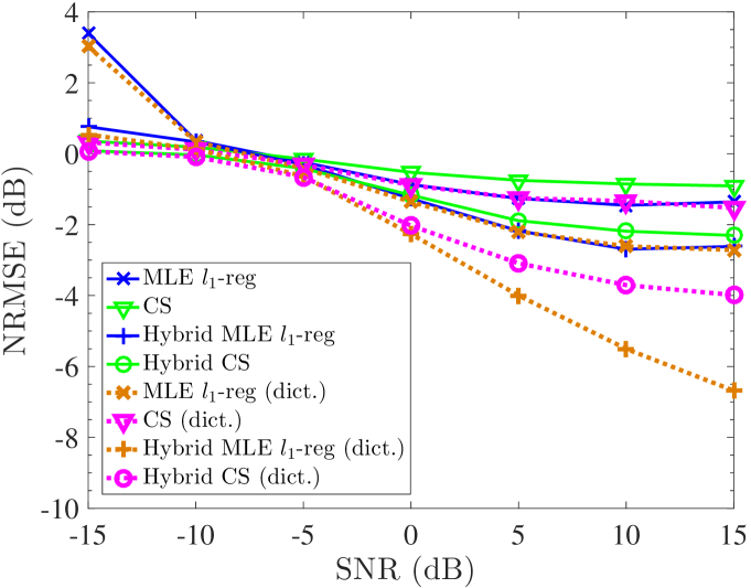
Figure 3: Comparison of NRMSE as a function of SNR for BS-based limited feedback schemes.

Fig. 3 shows the impact of quantization error for AoA and AoD. It can be seen that if the angles are drawn from the dictionaries there is no error due to angle quantization and the NRMSE of all studied algorithms becomes quite smaller (brown and magenda dotted curves) than the case where the angles are drawn uniformly in $[-\pi/2,\pi/2)$ (green and blue solid curves). The observation is that the impact of quantization error is severe for BS-based algorithms and their hybrid counterparts, so to compensate for this, larger dictionary sizes $G_{\rm T}$ and $G_{\rm R}$ will be utilized. In what follows, we always draw $\phi_{l},\phi_{l}^{\prime}\sim\mathcal{U}[-\pi/2,\pi/2)$, so there is always dictionary mismatch.

Fig. 4 compares LS-SQ, OMP-VQ, OMP-SQ, hybrid MLE $l_{1}$-regularized, and hybrid CS algorithms. To alleviate quantization errors, the proposed dictionary-based algorithms utilize $G_{\rm T}=G_{\rm R}=240$. Moreover we use $\overline{L}=15$ for the proposed limited feedback algorithms. For fair comparison, we set parameters so that the number of feedback bits is of the same order of magnitude for all algorithms considered. Note that for OMP-VQ the feedback overhead is not a function of $Q$ and thus it cannot be increased. Hybrid $l_{1}$-regularized MLE and hybrid CS are executed with $N_{\rm fb}=100$ and $N_{\rm fb}=120$, corresponding to $440$ and $496$ feedback bits, respectively. We set $Q=3$ (corresponding to $1548$ feedback bits) for LS-SQ, $Q=5$ (corresponding to $390$ feedback bits) for OMP-SQ, while OMP-VQ employs $273$ feedback bits with $2^{Q}$ phase states.

Figure 4: The proposed methods use fewer feedback bits yet outperform the LS baseline for all values of SNR.

Fig. 4 shows the NRMSE performance as a function of SNR. For SNR less than $-5$ dB the hybrid limited feedback schemes achieve the best NRMSE performance. In the very low SNR regime the hybrid CS algorithm offers the smallest NRMSE. For SNR greater than $6$ dB, OMP-SQ with $Q=5$ outperforms the other algorithms. The poor performance of LS-SQ stems from the fact that the soft estimate $\widehat{\mathbf{H}}_{\rm LS}$ before quantization is itself poor, as it does not exploit sparsity. OMP-VQ offers the worst performance across all algorithms in the high SNR regime. That happens because the VQ technique in [14] employs a predefined structured codebook at the BS, designed for Rayleigh fading. Although the proposed algorithms use fewer feedback bits than LS-SQ, they achieve much better performance due to their judicious design. For a moderate number of BS antennas, hybrid limited feedback algorithms are more suitable at low-SNR, while OMP-SQ is better at high-SNR.

VII-B NRMSE vs. $\overline{L}$

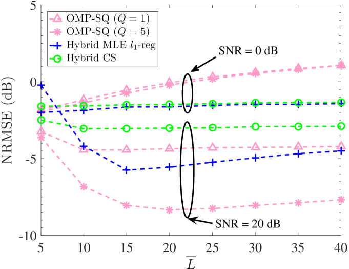
Figure 5: NRMSE versus $\overline{L}$ for the algorithms of setup 1 and 3. It can be seen that the NRMSE is not necessarily a decreasing function of $\overline{L}$.

Using the same parameters as in the previous paragraph, Fig. 5 studies the impact of the maximum number of OMP iterations, $\overline{L}$, on NRMSE performance of OMP-SQ and hybrid limited feedback algorithms under different values of SNR. It can be seen that in the low SNR regime the smaller $\overline{L}$ is, the smaller NRMSE can be achieved by all schemes. Namely, the smallest NRMSE is achieved for $\overline{L}=5$ for all algorithms. On the other hand, in the high SNR regime the NRMSE versus $\overline{L}$ curve has a convex shape with minimum around $\overline{L}\in[10,20]$ for all algorithms. This indicates that $\overline{L}$ should be chosen $\geq L$, but not much higher than $L$.

VII-C NRMSE vs. $G$ and $M_{\rm T}$

Next the impact of joint dictionary size, $G$, and the number of transmit antennas on NRMSE is studied for the proposed algorithms in Sections IV and VI. For this simulation, $M_{\rm R}=1$, $N_{\rm tr}=80$, and ${\rm SNR}=10$ dB. Hybrid schemes utilize $N_{\rm fb}=80$, the number of paths, the maximum number of OMP iterations, and the dimensionality reducing matrix are the same as in Section VII-A. OMP-SQ uses $Q=5$ bits per real number, and thus hybrid schemes and OMP-SQ utilize $160+15\mathsf{log}_{2}G$ and $150+15\mathsf{log}_{2}G$ feedback bits, respectively, in the worst case.

Figure 6: NRMSE as a function of the number of BS antennas for different joint dictionary sizes $G$. Higher $G$ improves NRMSE.

Fig. 6 studies the impact of $M_{\rm T}$ and $G$ on NRMSE. Recall that $G$ is determined from $G_{\rm T}$ and $G_{\rm R}$. Three different scenarios are considered for $G$, using $G_{\rm T}=G_{\rm R}=7$, $G_{\rm T}=G_{\rm R}=31$, and $G_{\rm T}=G_{\rm R}=127$. From Fig. 6 it is observed that for fixed $G$ increasing the number of transmit antennas yields higher NRMSE, while for fixed number of transmit antennas, using higher $G$ yields reduced NRMSE, as expected. Note that for $M_{\rm T}\geq 200$ OMP-SQ has the worst NRMSE performance, while for smaller $M_{\rm T}$ it achieves better NRMSE compared to hybrid schemes. For small $M_{\rm T}$, increasing $G$ significantly reduces the NRSME. For large $M_{\rm T}$, increasing $G$ has little impact on the NRMSE.

VII-D Beamforming Gain vs. SNR

Using the same parameters as in Section VII-A (Fig. 4) with $M_{\rm T}=128$, $M_{\rm R}=1$, and $P_{\rm T}=1$ Watt, in Fig. 7 we study the beamforming gain performance metric, defined as $\mathbb{E}\left[\frac{P_{\rm T}}{\|\widehat{\mathbf{h}}\|_{2}^{2}}\left|\mathbf{h}^{\mathsf{H}}\,\widehat{\mathbf{h}}\right|^{2}\right],$ as a function of SNR. This metric measures the similarity between the actual channel $\mathbf{h}$ and the normalized channel estimate $\widehat{\mathbf{h}}$ and is proportional to average received SNR. We also include the performance of perfect CSI to assess an upper bound on beamforming gain performance for the studied algorithms. Hybrid schemes of setup 3, OMP-VQ ($Q=5$), OMP-SQ ($Q=5$), LS-SQ ($Q=4$), and LS-VQ ($Q=5$) use $400$, $273$, $390$, $1024$, and $635$ feedback bits overhead, respectively. Interestingly, for ${\rm SNR}\geq 20$ dB OMP-SQ with $Q=5$ achieves the performance of perfect CSI. The proposed hybrid schemes have very similar but slightly worse performance relative to OMP-SQ. In addition, the performance gap between perfect CSI and the proposed algorithms is less than $1.5$ dB for ${\rm SNR}\geq 10$ dB. The proposed algorithms outperform LS schemes for all values of SNR. OMP-VQ performs very poorly compared to OMP-SQ and other hybrid schemes. OMP-SQ offers the best performance, but note that it assumes perfect knowledge of the SQ thresholds at the BS, which in reality depend on the unknown channel. Perhaps surprisingly, LS-VQ offers smaller beamforming gain than LS-SQ. One reason is that LS-SQ assumes perfect knowledge of the scalar quantization thresholds at the BS; another is that the vector-quantized codewords are confined to be PSK-codewords that lie on the $M_{\rm T}$-dimensional unit complex circle, so magnitude variation among the elements of $\widehat{\mathbf{h}}_{\rm LS}^{\mathsf{H}}$ cannot be exploited. We also note that the majority of VQ algorithms in the limited feedback literature, including LS-VQ, are designed for non-light-of-sight channels, a.k.a. Rayleigh fading, and the DD model used here is far from Rayleigh – so LS-VQ and OMP-VQ are not well-suited for the task.

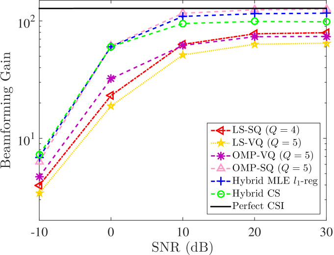
Figure 7: Beamforming gain as a function of SNR for $5$ different algorithms. The proposed methods outperform LS schemes for all values of SNR.

VII-E Beamforming Gain vs. $M_{\rm T}$

A more realistic channel scenario is considered next, based on the 3GPP multipath channel model [33], where path-loss and shadowing are also incorporated in the path gains $\alpha_{l}$. We assume a system operating at carrier frequency $F_{\rm car}=2$ GHz, and thus $\lambda\approx 0.15$. Transmit power and noise power are set $0.5$ Watts and $10^{-10}$ Watts, respectively. The number of paths is a discrete uniform RV in $[5,6,\ldots,19,20]$. For each path $l$: $\phi_{l},\phi_{l}^{\prime}\sim\mathcal{U}[-\pi/2,\pi/2)$, path distance $d_{l}\sim\mathcal{U}[80,120]$, common path-loss exponent $\eta\sim\mathcal{N}(2.8,0.1^{2})$, inverse path-loss $\rho_{l}=\left(\frac{\lambda}{4\pi}\right)^{2}\left(\frac{1}{d_{l}}\right)^{\eta}$, shadowing $10\mathsf{log}_{10}(v_{l})\sim\mathcal{N}(10\mathsf{log}_{10}(\rho_{l}),4^{2})$, and Rician parameter $\kappa_{l}\sim\mathcal{U}[0,50]$. Thus, the final multipath gain is given by $\alpha_{l}\sim\mathcal{CN}\!\left(\sqrt{\frac{\kappa_{l}}{\kappa_{l}+1}v_{l}},\frac{1}{\kappa_{l}+1}v_{l}\right)$, with path delay $\varphi_{l}\sim\mathcal{U}[0,2\pi]$. The average received SNR, incorporating path-losses, small- and large- scale fading effects, changes per realization, so an implicit averaging with respect to the received SNR is applied. The beamforming gain of all algorithms compared in Section VII is examined as a function of the number of transmit antennas. For this scenario we consider: $M_{\rm R}=1$ received antenna, $N_{\rm tr}=64$ training symbols, $\overline{L}=25$ for OMP and hybrid schemes, $N_{\rm fb}=N_{\rm tr}=64$ for all BS-based limited feedback algorithms and their hybrid counterparts, and $N_{\rm fb}$ columns of the DFT matrix were chosen for the dimensionality reducing matrix $\mathbf{P}$. The dictionary sizes were set to $G_{\rm T}=G_{\rm R}=180$.

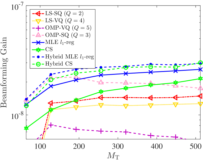
Figure 8: Beamforming gain as a function of $M_{\rm T}$ in the massive MIMO regime. The proposed algorithms outperform LS-SQ and LS-VQ for all values of $M_{\rm T}$.

Fig. 8 examines a massive MIMO scenario where $M_{\rm T}$ becomes very large. We observe that in this scenario the beamforming gain takes values of order $10^{-8}$. This is not surprising since on top of small-scale fading this scenario further incorporates path-loss and shadowing effects.

From Fig. 8 we note that hybrid $l_{1}$-regularized MLE achieves the best beamforming gain for almost all $M_{\rm T}$, while hybrid CS has very similar performance. OMP-SQ and OMP-VQ are the only algorithms whose performance decreases as the number of transmit antennas increases. It should be noted that OMP-VQ ($Q=5$), OMP-SQ (with $Q=3$), classic BS-based, and hybrid limited feedback schemes utilize only $428,$ $524$, $128$, and $502$, feedback bits overhead, respectively. MLE $l_{1}$-reg and CS have worse performance than their hybrid counterparts. On the other hand, LS-SQ (with $Q=2$), and LS-VQ (with $Q=4$), employ $4M_{\rm T}$ and $4(M_{\rm T}-1)$ feedback bits overhead, that is linear in $M_{\rm T}$. All proposed algorithms outperform LS schemes as they exploit the inherent sparsity of the DD channel, while the OMP-VQ algorithm offers very poor performance. It can be concluded that in the massive MIMO regime with realistic channel parameters, the BS-based limited feedback algorithms and their hybrid counterparts perform better than the other alternatives.

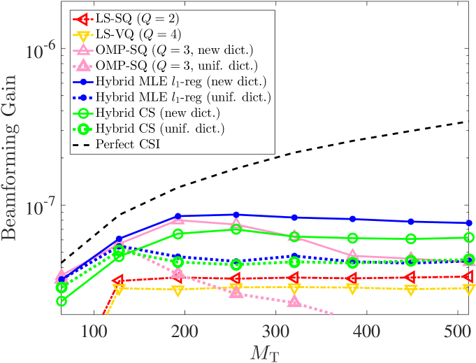
Figure 9: Beamforming gain vs $M_{\rm T}$ using 3GPP antenna directivity pattern at the BS. The directivity pattern-aware dictionary outperforms uniform dictionary.

Next Fig. 9 compares the proposed angle dictionary (labeled ‘new dict.’) and the uniform quantization dictionary (labeled ‘unif. dict.’) in the same massive MIMO scenario assuming that each BS antenna directivity pattern is given by Eq. (3) using $\phi_{\rm 3dB}=55^{o}$, $\mathtt{A}_{\rm m}=30$ dB, and $\mathtt{G}_{\rm dB}=8$ dBi [23]. All algorithms are configured with the same parameters as in the previous paragraph. From Fig. 9 is evident that for the same number of dictionary elements, the proposed non-uniform directivity-based dictionary offers considerably higher beamforming gain performance compared to the uniform one. In contrast to LS schemes, as the number of transmit antennas increases, the feedback overhead for the proposed algorithms remains unaffected, rendering them a promising option for massive MIMO systems.

VII-F Execution Time vs. $M_{\rm T}$

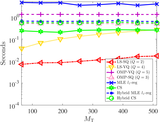
Figure 10: Execution time as a function of $M_{\rm T}$ in the massive MIMO regime.

For the pragmatic simulation setting of Fig. 8, Fig. 10 measures the end-to-end execution time of all algorithms averaged over 200 independent experiments. It can be seen that MLE-reg algorithm of setup 2 requires approximately 4 seconds for all values of $M_{\rm T}$, which is the highest execution time. OMP-VQ algorithm requires approximately 1.3 seconds for all studied values of $M_{\rm T}$. Hybrid schemes and OMP-SQ offer end-to-end execution time of 0.5 seconds for all values of $M_{\rm T}$, while CS scheme of setup 2 can reduce the execution time to the half, requiring 0.25 seconds. As can be seen in Fig. 10 the execution time of the above algorithms remains unaffected by the number of BS antennas. On the contrary, the execution time of the baseline LS schemes increases with the number of BS antennas. The execution time of LS schemes is the smallest among all algorithms. When the number of BS antennas is moderate, LS-SQ and LS-VQ require execution time in the order of 0.01 seconds, while in the massive MIMO regime their execution time increases to 0.017 and 0.25 seconds respectively. The low execution time of LS-SQ stems form the fact that it requires a calculation of a pseudoinverse followed by the execution of Lloyd’s algorithm using the build-in Matlab functions.

VII-G Multiuser Sum-Capacity vs. $P_{\rm T}$

In practice, cellular systems serve concurrently multiple UE terminals at the same time, so a multiuser performance metric is of significant interest. Towards this end, we consider the downlink sum-capacity of a cellular network under zero-forcing ZF beamforming as a function of $P_{\rm T}$, assuming $M_{\rm T}=256$, $K=16$ scheduled UEs, $M_{\rm R}=1$, and $N_{\rm tr}=80$. Hybrid schemes and OMP algorithms employ $\overline{L}$, $G_{\rm T}=210$ and $G_{\rm R}=180$ elements. BS uses a data stream of dimension $K$, $\mathbf{u}\in\mathds{C}^{K}$. After receiving the feedback from $K$ UEs, BS estimates the downlink channels for each user $k$, $\widehat{\mathbf{h}}_{k}^{\mathsf{H}}$, forms the compound downlink channel matrix $\widehat{\mathbf{T}}=\left[\widehat{\mathbf{h}}_{1}~{}\widehat{\mathbf{h}}_{2}~{}\ldots~{}\widehat{\mathbf{h}}_{K}\right]^{\mathsf{H}}.$ Under ZF precoding with equal power allocation $\frac{P_{\rm T}}{K}$ per user, precoding matrix $\mathbf{V}$ is given by $\mathbf{V}=[\mathbf{v}_{1}~{}\mathbf{v}_{2}~{}\ldots~{}\mathbf{v}_{K}]=\mathtt{t}\left(\widehat{\mathbf{T}}^{\mathsf{H}}\widehat{\mathbf{T}}\right)^{-1}\widehat{\mathbf{T}}^{\mathsf{H}},$ where $\mathtt{t}^{2}={\frac{K}{\mathsf{trace}\!\left(\left(\widehat{\mathbf{T}}^{\mathsf{H}}\widehat{\mathbf{T}}\right)^{-1}\right)}}$ guarantees that precoding vector satisfies the power constraint. BS transmits $\mathbf{s}=\mathbf{V}\mathbf{u}$. The corresponding instantaneous signal-to-interference-plus-noise-ratio (SINR) for user $k$ is given by $\gamma_{k}=\frac{P_{\rm T}\left|\mathbf{h}_{k}^{\mathsf{H}}{\mathbf{v}}_{k}\right|^{2}}{\sum\limits_{k^{\prime}\neq k}P_{\rm T}\left|\mathbf{h}_{k}^{\mathsf{H}}{\mathbf{v}}_{k^{\prime}}\right|^{2}+K\,\sigma^{2}}.$ The achievable ergodic rate for user $k$ is given by $\mathbb{E}[\mathsf{R}(\gamma_{k})]=\left(1-\frac{N_{\rm tr}}{U_{\rm c}}\right)\mathbb{E}[\mathsf{log}_{2}(1+\gamma_{k})].$ The achievable ergodic sum-rate (sum-capacity) for $K$ scheduled UEs is expressed as $\sum_{k=1}^{K}\mathbb{E}[\mathsf{R}(\gamma_{k})]$.

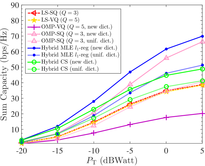
Figure 11: Downlink sum-capacity as a function of the BS transmit power. The proposed limited feedback along with non-uniform directional dictionaries schemes offer significant sum-capacity performance gains.

TABLE I: Complexity analysis and number of feedback bits.

	Complexity at the BS	Complexity at the UE	Feedback Bits
LS-SQ	$\mathcal{O}(M_{\rm T}\,M_{\rm R})$	$\mathcal{O}\!\left(I_{\rm SQ}\,2^{Q}\,M_{\rm T}\,M_{\rm R}+N_{\rm tr}^{2}(M_{\rm T}+N_{\rm tr})\right)$	$2\,Q\,M_{\rm T}\,M_{\rm R}$
LS-VQ	$\mathcal{O}(1)$	$\mathcal{O}\!\left(M_{\rm T}\,\mathsf{log}(M_{\rm T})+N_{\rm tr}^{2}(M_{\rm T}+N_{\rm tr})\right)$	$Q\,(M_{\rm T}-1)$
OMP-SQ	$\mathcal{O}(\overline{L}\,M_{\rm T}\,M_{\rm R})$	$\mathcal{O}\!\left(I_{\rm SQ}\,2^{Q}\,\overline{L}+\overline{L}\,M_{\rm R}\,N_{\rm tr}(\overline{L}+G)\right)$	$\overline{L}(\lceil\mathsf{log}_{2}G\rceil+2Q)$
OMP-VQ	$\mathcal{O}(\overline{L}(M_{\rm T}\,M_{\rm R}+2^{5+Q}))$	$\mathcal{O}\!\left(2^{5+Q}\,\overline{L}+\overline{L}\,M_{\rm R}\,N_{\rm tr}(\overline{L}+G)\right)$	$\overline{L}(\lceil\mathsf{log}_{2}G\rceil+2)+3$
CS	$\mathcal{O}\!\left(G(N_{\rm fb}+M_{\rm T}\,M_{\rm R})\right)$	$N_{\rm fb}\,M_{\rm R}\,N_{\rm tr}$	$2N_{\rm fb}$
MLE-reg	$\mathcal{O}\!\left(G((I_{\rm max}+N_{\rm fb})N_{\rm fb}+M_{\rm T}\,M_{\rm R})\right)$	$N_{\rm fb}\,M_{\rm R}\,N_{\rm tr}$	$2N_{\rm fb}$
Hybrid CS	$\mathcal{O}\!\left(\overline{L}(N_{\rm fb}+M_{\rm T}\,M_{\rm R})\right)$	$\mathcal{O}\!\left(N_{\rm fb}\,M_{\rm R}\,N_{\rm tr}+\overline{L}\,M_{\rm R}\,N_{\rm tr}(\overline{L}+G)\right)$	$2N_{\rm fb}+\overline{L}\lceil\mathsf{log}_{2}G\rceil$
Hybrid MLE-reg	$\mathcal{O}\!\left(\overline{L}((I_{\rm max}+N_{\rm fb})N_{\rm fb}+M_{\rm T}\,M_{\rm R})\right)$	$\mathcal{O}\!\left(N_{\rm fb}\,M_{\rm R}\,N_{\rm tr}+\overline{L}\,M_{\rm R}\,N_{\rm tr}(\overline{L}+G)\right)$	$2N_{\rm fb}+\overline{L}\lceil\mathsf{log}_{2}G\rceil$

Fig. 11 depicts the downlink sum-capacity as a function of BS transmit power $P_{\rm T}$. The downlink channels for each user are generated using the same parameters as in Section VII-E with antenna directivity pattern parameters $\phi_{\rm 3dB}=55^{o}$, $\mathtt{A}_{\rm m}=30$ dB, and $\mathtt{G}_{\rm dB}=8$ dBi. The coherence block occupies 20 resource blocks, i.e., $U_{\rm c}=1680$ channel uses. The following algorithms are compared: LS-SQ with $Q=3$, LS-VQ with $Q=5$, OMP-VQ with $Q=5$, OMP-SQ with $Q=3$, and hybrid schemes using the proposed dictionaries (labeled ‘new dict.’) and uniform dictionaries (labeled ‘unif. dict.’). The performance gains of the proposed non-uniform dictionaries over conventional uniform ones are evident in Fig. 11, especially for MLE-reg and OMP-SQ algorithms. For $1$ Watt transmission power, MLE-reg and OMP-SQ with proposed non-uniform dictionaries offer $15$ and $20$ bit/sec/Hz higher capacity than MLE-reg and OMP-SQ executed with uniform dictionaries. The proposed methods in conjunction with non-uniform dictionaries offer a substantial sum-capacity performance gain compared to LS schemes. The performance of OMP-VQ is very poor, at least $5$ dB worse than proposed MLE-reg algorithm with non-uniform dictionaries for all values of $P_{\rm T}$.

VII-H Complexity Analysis

In this section a detailed computational complexity analysis at both UE and BS is presented for all studied algorithms. Table I shows the computational cost of all studied algorithms along with the required number of feedback bits.

For LS schemes, at the UE side the calculation of $\widehat{\mathbf{H}}_{\rm LS}$ requires $\mathcal{O}(N_{\rm tr}^{2}(M_{\rm T}+N_{\rm tr}))$ arithmetic operations. For LS-SQ, at the UE side, for each element of $\widehat{\mathbf{H}}_{\rm LS}$, $\mathcal{O}(I_{\rm SQ}\,2^{Q})$ computations are required for the SQ algorithm, where $I_{\rm SQ}$ is the maximum of iterations for algorithm to converge. After receiving the associated indices and the elements of the quantized channel, the BS reconstructs the channel with complexity $\mathcal{O}(M_{\rm T}\,M_{\rm R})$. For LS-VQ, at the UE side, the computational cost is due to the calculation of $\widehat{\mathbf{H}}_{\rm LS}$ and the computation of optimal $M_{\rm T}$-dimensional $2^{Q}$-PSK sequence, which requires $\mathcal{O}(M_{\rm T}\,\mathsf{log}(M_{\rm T}))$ computations [13]. Since the codebook is already stored at the BS the channel reconstruction requires $\mathcal{O}(1)$ computations. The complexity of OMP algorithm is dominated by lines 4, 7, and 8 in Algorithm 1, which is $\overline{L}\,M_{\rm R}\,N_{\rm tr}(\overline{L}+G))$. Hence, the complexity for OMP-SQ is $\mathcal{O}\!\left(I_{\rm SQ}\,2^{Q}\,\overline{L}+\overline{L}\,M_{\rm R}\,N_{\rm tr}(\overline{L}+G)\right)$. At the BS, the reconstruction of the channel matrix for OMP-SQ exploits the sparsity of channel vector $\widehat{\mathbf{g}}$, and thus using only the $\overline{L}$ non-zero elements of sparse matrix $\widehat{\mathbf{G}}$ the channel reconstruction using (8) requires only $\mathcal{O}(\overline{L}\,M_{\rm T}\,M_{\rm R})$ arithmetic operations. The complexity of the algorithm in [14] at the UE side is due to the vector quantization of the $\overline{L}$ non-zero elements of path coefficient vector $\widehat{\mathbf{g}}$ through Viterbi algorithm ($2^{5+Q}\overline{L}$ operations) and the support identification of $\widehat{\mathbf{g}}$ through OMP algorithm. Hence, OMP-VQ algorithm requires total $\mathcal{O}\!\left(2^{5+Q}\,\overline{L}+\overline{L}\,M_{\rm R}\,N_{\rm tr}(\overline{L}+G)\right)$ arithmetic operations at the UE. At the BS side, OMP-VQ algorithm reconstructs the non-zero elements of $\widehat{\mathbf{g}}$ through the Viterbi algorithm, requiring $O(2^{5+Q}\,\overline{L})$ computations; whereas the reconstruction of the actual channel, using (8), demands $\mathcal{O}(\overline{L}\,M_{\rm T}\,M_{\rm R})$ arithmetic operations. BS-based limited feedback schemes require $N_{\rm fb}\,M_{\rm R}\,N_{\rm tr}$ arithmetic operations at the UE side due to the multiplication of $\mathbf{P}^{\mathsf{H}}$ with $\mathbf{y}$. While hybrid schemes require an extra $\overline{L}\,M_{\rm R}\,N_{\rm tr}(\overline{L}+G))$ computational cost at the UE side due to the execution of OMP algorithm for support identification. At the BS side, as shown in Sections V-A and V-B, CS and MLE-reg algorithms require $\mathcal{O}(G\,N_{\rm fb})$ and $\mathcal{O}((I_{\rm max}+N_{\rm fb})G\,N_{\rm fb})$ computations, respectively, to obtain an estimate of vector $\mathbf{x}$. In addition, an extra $\mathcal{O}(G\,M_{\rm T}\,M_{\rm R})$ computational cost is required to reconstruct the actual channel through (8). Finally, hybrid schemes require at the BS, $\mathcal{O}(\overline{L}\,N_{\rm fb})$ for CS and $\mathcal{O}((I_{\rm max}+N_{\rm fb})\overline{L}\,N_{\rm fb})$ for MLE-reg algorithms. Using the support information obtained from feedback, hybrid schemes require extra $\mathcal{O}(\overline{L}M_{\rm T}\,M_{\rm R})$ calculations to evaluate (8) for channel reconstruction.

VII-I Take-home Points from the Simulations

We close this section by summarizing the most important take-home points from our numerical results.

The baseline quantization algorithms LS-SQ and LS-VQ require low execution time but their feedback overhead scales linearly with the number of BS antennas. As they don’t exploit the DD parameterization, LS-SQ and LS-VQ yield worse estimation accuracy compared to the proposed limited feedback algorithms of setups 1, 2, and 3, even though LS-SQ/VQ use a higher number of feedback bits. OMP-VQ requires relative execution time and feedback overhead, depending linearly on $\overline{L}$ and logarithmically on $G$; it performs very poorly in all our simulation scenarios. The principal reason for the poor performance for OMP-VQ is that its codewords are pre-defined and fixed, offering limited channel estimation granularity. The proposed algorithms of setup 2 require $2N_{\rm fb}\leq 2N_{\rm tr}M_{\rm R}$ feedback bits, independent of the number of BS antennas. The execution time of one-bit MLE-reg is high, whereas the execution time of one-bit CS is at least an order of magnitude lower; on the other hand, the estimation performance of one-bit CS is worse compared to one-bit MLE-reg. Both algorithms of setup 2 have slightly worse estimation performance than OMP-SQ for moderate number of BS antennas in the high SNR regime. Conversely, in the low SNR regime or when the number of BS antennas increases, one-bit CS and one-bit MLE-reg outperform OMP-SQ. Moreover, the algorithms of setup 2 perform slightly worse compared to their hybrid counterparts of setup 3. Such performance gains of hybrid schemes come at the cost of an extra $\overline{L}\lceil\mathsf{log}_{2}G\rceil$ bits in feedback overhead.

We found that employing joint dictionary size $G=\mathcal{O}(M_{\rm T}M_{\rm R})$ suffices to obtain good channel estimation accuracy for the dictionary-based algorithms, corroborating the findings of dictionary-based estimation prior art [20, 21, 24]. Consequently, the feedback overhead for massive MIMO systems employing the proposed OMP-SQ and hybrid schemes, scales as $\mathcal{O}(\overline{L}\,(\mathsf{log}(M_{\rm T}M_{\rm R})+2Q))$ and $\mathcal{O}(\overline{L}\,\mathsf{log}(M_{\rm T}M_{\rm R})+2N_{\rm fb})$, respectively. This logarithmic scaling with the number of BS antennas underscores the practicality of the proposed limited feedback algorithms for the DD model in massive MIMO scenarios.

VIII Conclusion and Future Work

This work provided a new limited feedback framework using dictionary-based sparse channel estimation algorithms that entail low computational complexity, and thus can be implemented in real-time. The proposed dictionary accounts for the antenna directivity pattern and can offer beamforming and capacity gains while requiring less feedback overhead compared to uniform dictionaries. Unlike VQ-based schemes for which the number of feedback bits must grows linearly with the number of BS antennas to maintain a certain performance level, the number of feedback bits for the proposed algorithms is under designer control, and they can achieve better performance using a substantially lower bit budget. The proposed baseline OMP-SQ algorithm (setup 1) achieves the best performance when the number of transmit antennas is moderate and SNR is high, while in the low-SNR regime the BS-based (setup 2) and hybrid (setup 3) schemes offer better performance. The hybrid schemes (setup 3) achieve the best performance in the massive MIMO regime.

References

- [1] J. Hoydis, S. ten Brink, and M. Debbah, “Massive MIMO in the UL/DL of cellular networks: How many antennas do we need?” IEEE J. Sel. Areas Commun., vol. 31, no. 2, pp. 160–171, Feb. 2013.
- [2] T. L. Marzetta, “Noncooperative cellular wireless with unlimited numbers of base station antennas,” IEEE Trans. Wireless. Comm., vol. 9, no. 11, pp. 3590–3600, Nov. 2010.
- [3] F. Rusek et al., “Scaling up MIMO: Opportunities and challenges with very large arrays,” IEEE Signal Process. Mag., vol. 30, no. 1, pp. 40–60, Jan. 2013.
- [4] H. Q. Ngo, E. G. Larsson, and T. L. Marzetta, “Energy and spectral efficiency of very large multiuser MIMO systems,” IEEE Trans. Commun., vol. 61, no. 4, pp. 1436–1449, Apr. 2013.
- [5] N. Jindal, “MIMO broadcast channels with finite-rate feedback,” IEEE Trans. Inf. Theor., vol. 52, no. 11, pp. 5045–5060, Nov. 2006.
- [6] G. Caire, N. Jindal, M. Kobayashi, and N. Ravindran, “Multiuser MIMO achievable rates with downlink training and channel state feedback,” IEEE Trans. Inf. Theor., vol. 56, no. 6, pp. 2845–2866, Jun. 2010.
- [7] A. Adhikary, J. Nam, J.-Y. Ahn, and G. Caire, “Joint spatial division and multiplexing—the large-scale array regime,” IEEE Trans. Inf. Theor., vol. 59, no. 10, pp. 6441–6463, Oct. 2013.
- [8] E. Dahlman, S. Parkvall, and J. Skold, 4G, LTE-Advanced Pro and The Road to 5G. Elsevier Science, 2016.
- [9] H. Ji et al., “Overview of full-dimension MIMO in LTE-Advanced Pro.” CoRR, 2016.
- [10] D. J. Love, R. W. Heath, V. K. Lau, D. Gesbert, B. D. Rao, and M. Andrews, “An overview of limited feedback in wireless communication systems,” IEEE J. Sel. Areas Commun., vol. 26, no. 8, pp. 1341–1365, Oct. 2008.
- [11] K. K. Mukkavilli, A. Sabharwal, E. Erkip, and B. Aazhang, “On beamforming with finite rate feedback in multiple-antenna systems,” IEEE Trans. Inf. Theor., vol. 49, no. 10, pp. 2562–2579, Oct. 2003.
- [12] V. Lau, Y. Liu, and T.-A. Chen, “On the design of MIMO block-fading channels with feedback-link capacity constraint,” IEEE Trans. Commun., vol. 52, no. 1, pp. 62–70, Jan. 2004.
- [13] D. J. Ryan, I. V. L. Clarkson, I. B. Collings, D. Guo, and M. L. Honig, “QAM and PSK codebooks for limited feedback MIMO beamforming,” IEEE Trans. Commun., vol. 57, no. 4, pp. 1184–1196, Apr. 2009.
- [14] J. Choi, Z. Chance, D. J. Love, and U. Madhow, “Noncoherent trellis coded quantization: A practical limited feedback technique for massive MIMO systems,” IEEE Trans. Commun., vol. 61, no. 12, pp. 5016–5029, Dec. 2013.
- [15] P. Xia and G. Giannakis, “Design and analysis of transmit-beamforming based on limited-rate feedback,” IEEE Trans. Signal Process., vol. 54, no. 5, pp. 1853–1863, May 2006.
- [16] K. Huang, R. W. Heath Jr, and J. G. Andrews, “Limited feedback beamforming over temporally-correlated channels,” IEEE Trans. Signal Process., vol. 57, no. 5, pp. 1959–1975, May 2009.
- [17] O. Mehanna and N. D. Sidiropoulos, “Channel tracking and transmit beamforming with frugal feedback,” IEEE Trans. Signal Process., vol. 62, no. 24, pp. 6402–6413, Dec. 2014.
- [18] T. L. Marzetta and B. M. Hochwald, “Fast transfer of channel state information in wireless systems.” IEEE Trans. Signal Process., vol. 54, no. 4, pp. 1268–1278, Apr. 2006.
- [19] Z. Jiang, A. F. Molisch, G. Caire, and Z. Niu, “Achievable rates of FDD massive MIMO systems with spatial channel correlation,” IEEE Trans. Wireless. Comm., vol. 14, no. 5, pp. 2868–2882, May 2015.
- [20] W. U. Bajwa, J. Haupt, A. M. Sayeed, and R. Nowak, “Compressed channel sensing: A new approach to estimating sparse multipath channels,” Proc. IEEE, vol. 98, no. 6, pp. 1058–1076, Jun. 2010.
- [21] R. W. Heath, N. Gonzalez-Prelcic, S. Rangan, W. Roh, and A. M. Sayeed, “An overview of signal processing techniques for millimeter wave MIMO systems,” IEEE J. Sel. Topics Signal Process., vol. 10, no. 3, pp. 436–453, May 2016.
- [22] 3GPP TS 36.101 V13.2.1, “Evolved universal terrestrial radio access (E-UTRA); User Equipment (UE) radio transmission and reception, Release 13,” May 2016.
- [23] A. Kammoun, H. Khanfir, Z. Altman, M. Debbah, and M. Kamoun, “Preliminary results on 3D channel modeling: From theory to standardization,” IEEE J. Sel. Areas Commun., vol. 32, no. 6, pp. 1219–1229, Jun. 2014.
- [24] R. Méndez-Rial, C. Rusu, N. González-Prelcic, A. Alkhateeb, and R. W. Heath, “Hybrid MIMO architectures for millimeter wave communications: Phase shifters or switches?” IEEE Access, vol. 4, pp. 247–267, Jan. 2016.
- [25] J. Mo, P. Schniter, N. G. Prelcic, and R. W. Heath, “Channel estimation in millimeter wave MIMO systems with one-bit quantization,” in Proc. Asilomar Conf. on Signals, Systems and Computers (Asilomar), Pacific Grove, CA, 2014, pp. 957–961.
- [26] C. Rusu, R. Méndez-Rial, N. González-Prelcic, and J. R. W. Heath, “Adaptive one-bit compressive sensing with application to low-precision receivers at mmWave,” in Proc. IEEE Global Telecommunications Conf. (GLOBECOM), San Diego, CA, Dec. 2015.
- [27] Z. Zhou, X. Chen, D. Guo, and M. L. Honig, “Sparse channel estimation for massive MIMO with 1-bit feedback per dimension,” in Proc. IEEE Wireless Commun. and Networking Conf. (WCNC), San Francisco, CA, 2017.
- [28] J. A. Tropp and A. C. Gilbert, “Signal recovery from random measurements via orthogonal matching pursuit,” IEEE Trans. Inf. Theor., vol. 53, no. 12, pp. 4655–4666, Dec. 2007.
- [29] J. W. Choi, B. Shim, Y. Ding, B. Rao, and D. In Kim, “Compressed sensing for wireless communications : Useful tips and tricks,” ArXiv e-prints, Nov. 2015.
- [30] Y. Nesterov, Introductory lectures on convex optimization : a basic course, ser. Applied optimization. Boston, Dordrecht, London: Kluwer Academic Publ., 2004.
- [31] B. O’Donoghue and E. Candès, “Adaptive restart for accelerated gradient schemes,” Foundations of Computational Mathematics, vol. 15, no. 3, pp. 715–732, 2015.
- [32] R. M. Gray and D. L. Neuhoff, “Quantization,” IEEE Trans. Inf. Theor., vol. 44, no. 6, pp. 2325–2383, Oct. 1998.
- [33] 3GPP TS 36.814 V9.0.0, “Evolved universal terrestrial radio access (E-UTRA); Further advancements for E-UTRA physical layer aspects, Release 9,” Mar. 2010.
- [34] P. N. Alevizos, X. Fu, N. Sidiropoulos, Y. Yang, and A. Bletsas, “Non-uniform directional dictionary-based limited feedback for massive MIMO systems,” in Proc. IEEE International Symposium on Modeling and Optimization in Mobile, Ad Hoc, and Wireless Networks (WiOpt), Paris, FR, May 2017.
- [35] S. Sesia, I. Toufik, and M. Baker, LTE - The UMTS Long Term Evolution: From Theory to Practice. Wiley, 2011. [Online]. Available: https://books.google.es/books?id=beIaPXLzYKcC
- [36] 3GPP TR 37.840 V12.1.0, “Technical Specification Group Radio Access Network; Study of Radio Frequency (RF) and Electromagnetic Compatibility (EMC) requirements for Active Antenna Array System (AAS) base station, Release 12,” Dec. 2013.
- [37] T. Blumensath, “Accelerated iterative hard thresholding,” Signal Processing, vol. 92, no. 3, pp. 752–756, 2012.
- [38] S. Foucart and H. Rauhut, A Mathematical Introduction to Compressive Sensing. Birkhäuser Basel, 2013.
- [39] P. T. Boufounos and R. G. Baraniuk, “1-bit compressive sensing,” in Proc. IEEE Information Sciences and Systems (CISS), 2008, pp. 16–21.
- [40] Y. Plan and R. Vershynin, “One-bit compressed sensing by linear programming,” Communications on Pure and Applied Mathematics, vol. 66, no. 8, pp. 1275–1297, 2013.
- [41] L. Jacques, J. N. Laska, P. T. Boufounos, and R. G. Baraniuk, “Robust 1-bit compressive sensing via binary stable embeddings of sparse vectors,” IEEE Trans. Inf. Theor., vol. 59, no. 4, pp. 2082–2102, Apr. 2013.
- [42] L. Zhang, J. Yi, and R. Jin, “Efficient algorithms for robust one-bit compressive sensing,” in Proc. International Conference on Machine Learning (ICML), Beijing, China, Jun. 2014, pp. 820–828.
- [43] E. Tsakonas, J. Jaldén, N. D. Sidiropoulos, and B. Ottersten, “Sparse conjoint analysis through maximum likelihood estimation,” IEEE Trans. Signal Process., vol. 61, no. 22, pp. 5704–5715, Nov. 2013.
- [44] S. Boyd and L. Vandenberghe, Convex Optimization. New York, NY, USA: Cambridge University Press, 2004.
- [45] D. P. Bertsekas, Convex optimization algorithms. Nashua, NH: Athena Scientific, 2015.
- [46] A. Beck and M. Teboulle, “A fast iterative shrinkage-thresholding algorithm for linear inverse problems,” SIAM journal on imaging sciences, vol. 2, no. 1, pp. 183–202, 2009.