Low-Level Augmented Bayesian Optimization for Finding the Best Cloud VM

Abstract

With the advent of big data applications, which tends to have longer execution time, choosing the right cloud VM to run these applications has significant performance as well as economic implications. For example, in our large-scale empirical study of 107 different workloads on three popular big data systems, we found that a wrong choice can lead to a 20 times slowdown or an increase in cost by 10 times.

Bayesian optimization is a technique for optimizing expensive (black-box) functions. Previous attempts have only used instance-level information (such as # of cores, memory size) which is not sufficient to represent the search space. In this work, we discover that this may lead to the fragility problem—either incurs high search cost or finds only the sub-optimal solution. The central insight of this paper is to use low-level performance information to augment the process of Bayesian Optimization. Our novel low-level augmented Bayesian Optimization is rarely worse than current practices and often performs much better (in 46 of 107 cases). Further, it significantly reduces the search cost in nearly half of our case studies.

Based on this work, we conclude that it is often insufficient to use general-purpose off-the-shelf methods for configuring cloud instances without augmenting those methods with essential systems knowledge such as CPU utilization, working memory size and I/O wait time.

I Introduction

Motivation. Cloud computing is a cost-effective alternative to on-premise computing. To accommodate diverse workloads, cloud service providers (Amazon, Google, and Azure) offer over 100 virtual machines (VM) types [1]. Our experiments show the optimal choice of VMs can be up to 20 times faster and 10 times less expensive than the worst VM for the same workload. Therefore, choosing the right VM type for a workload is essential to provide quality service while being commercially competitive [2, 3].

In this paper, we address the problem of finding a suitable cloud VM type for a recurring job. This problem is further aggravated by the long execution times of the workloads since a brute-force approach will no longer be a viable option. Furthermore, because there are charges to evaluate, this decision space must be explored efficiently. The prior work in this area, solved this problem using two different approaches namely (1) PARIS [1] builds a complex performance model (using large-scale one-time benchmark data) to predict workload performance, and (2) CherryPick [4] uses Bayesian optimization to find the best cloud configuration. We prefer the Bayesian Optimization (BO) method because it does not require additional historical training data and supports any objective functions (essential for diverse workloads).

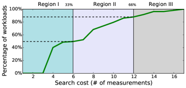
Figure 1: The number of measurements required by Bayesian Optimization (as used in  [4]) to find the optimal VM type. We observe that 50% and 85% of the workloads (shown in dashed lines) require 6 (33% of the search space) and 12 (66% of the search space) measurements respectively. Bayesian Optimization is not always effective for any workload. The fragility problem—either incurs high search cost or yields sub-optimal solution (as in Region II and Region III.

However, we have come across workloads where a BO method is ineffective—surprisingly, we found this problem in a large number of workloads. Our large-scale empirical study, as shown in Figure  1, reveals that BO incurs different search cost on different workloads. We observe that BO is effective in 50% of the workloads (in Region I) since it requires exploration of only 33% of the total search space. However, we also notice that BO is not as effective at finding the optimal VM type for the other workloads (in Region II and Region III). This poor performance can be attributed to the insufficient information (for example # of cores, memory, etc.) used by BO during the search process. Such VM characteristics are not sufficient to capture application behavior [5, 1, 6]. Consequently, BO may fail to find the optimal VM for some workloads efficiently. Figure 2 shows how BO is sluggish to find a ‘better’ VM type for a workload from the Region III. In summary, the lesson that we learned from the large-scale empirical study is BO is not a silver bullet to find optimal VM type for any workloads. Furthermore, it can be fragile—either incurs higher search cost or yields a sub-optimal solution. Without further investigation, it is hard to claim BO is an effective method for finding the best VM type.

Our Work. To further understand the fragility of Bayesian Optimization, we conducted a large-scale empirical study with three popular big data systems along with 107 different workloads and 18 different VM types (for more details refer to Section II-B). We first observe that using rule-of-thumbs (intuitions) to select the best VM type is far from ideal. There does not exist one such best VM type for all the workloads. Second, the same application with different input sizes may favor different VM types. Last, while the execution time tends to decrease with a more powerful VM, the cost per unit time goes up, which compresses the deployment costs. This creates a level playing field—several inferior configurations in execution time are now competitive in deployment cost. These reasons make the problem of selecting the best VM for any given workload challenging.

To find the best VM type, CherryPick [4] uses Bayesian Optimization, which sequentially evaluates the VMs and moves closer to the optimal VM type. As presented before, a BO method can encounter the fragility problem. As shown in Figure 2, the performance of instance found after the fifth iteration is 1.75 times slower when compared to the optimal instance type. In this case, BO did not find the optimal solution until the thirteenth attempt. We argue that the fragility of BO arises from the insufficient information. That is, characteristics of a VM such as CPU speed, core counts, memory per core and disk capacity, is not sufficient to predict its performance. Besides, the choice of the kernel function (the prior) and the selection of the initial measurements are both critical to the effectiveness of BO [7, 8, 9, 10]. We believe they are also related to the fragility problem.

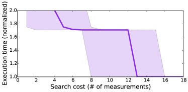
Figure 2: Using Bayesian Optimization to find the best VM type for running the ALS algorithm on Spark. The horizontal axis represents the search cost, and the vertical axis represents the execution time of the workload (both are lower the better). A naive Bayesian Optimization method progresses slowly towards the optimal VM type. The low-level augmented BO method alleviates the fragility problem as shown in Figure 10(a).

Low-level performance metrics are a good proxy for estimating application and system performance [5, 1]. They are also useful to identify performance anomalies  [11, 12]. We argue that low-level performance information such as I/O wait and memory usage better captures application behavior and better guides a BO method through the search process.

In this paper, we proposed a novel method to augment Bayesian Optimization by leveraging low-level performance information. However, embedding low-level performance information is tricky since the (low-level) information is not available until the workload is executed on a given VM type. Our proposed modeling technique seamlessly integrates the high-level features with the low-level performance information. The prediction model estimates the workload performance in VMs (not measured) using the low-level performance information collected from previous measurements. Throughout the search process, the model keeps updating the belief based on the new measurements.

The proposed low-level augmented Bayesian Optimization (Augmented BO) outperforms the naive Bayesian Optimization (Naive BO) [4]. Our evaluation shows a reduction in search cost on 46 out of 107 applications in search for the most cost-effective configuration. Our method reduces about 20% search cost on average for cases with the fragility issue, and reaches 43% reduction for some while maintaining the same or slightly better performance in comparison to Naive BO.

Summary and contributions. Our key contributions are:

1. A large-scale empirical study to analyze the performance of Bayesian Optimization on a wide range of realistic data analytics and machine learning workloads (Section II);

2. A demonstration of fragility of BO to find the suitable instance for a specific workload (Section III);

3. A novel low-level augmented Bayesian Optimization method to alleviate the fragility problem (Section IV).

II Background and Motivation

In this section, we present the challenges of selecting the best VM type. We also formulate our problem setting and explain why search-based optimization is more desirable.

II-A Problem Formalization

A cloud service provider presents its user with several choices of VM types ($\mathit{VM}$). Let $\mathit{VM}_{i}$ indicate the $i^{th}$ VM type in the list of VMs, which takes value from a finite domain $Dom(\mathit{VM}_{i})$. In general, $\mathit{VM}_{i}$ indicates the published characteristics of VMs (such as memory size, # of cores). $\mathit{VM}_{ij}$ represents the $j^{th}$ characteristic of the $i^{th}$ VM type. The instance space is thus $Dom(\mathit{VM}_{1})\times Dom(\mathit{VM}_{2})\times...\times Dom(\mathit{VM}_{n})$, which is the Cartesian product of the domains, where $n=\left|{\mathit{VM}}\right|$ is the number of VMs provided by the cloud service provider. When a workload ($w\in W$) is run on a VM ($\mathit{VM}_{i}$), the low-level metrics ($l_{i,w}\in L$) can be collected from the VM. Each VM type ($\mathit{VM}$) has a corresponding performance measure $y\in Y$ (e.g., time or cost). We denote the performance measure associated with a given VM type and a workload by $y_{i,w}=f(\mathit{VM}_{i,w})$. In this setting, $\mathit{VM}_{i,w}$ and $y_{i,w}$ is called independent and dependent variable respectively.

Our goal is design a search method to:

1. Minimize performance difference between the best VM ($\mathit{VM^{*}}$) (found by search) and the optimal VM ($\mathit{VM}^{opt})$. We find $\mathit{VM^{*}}$ both in terms of execution time and deployment cost;

2. Minimize search cost—the number of measurements required to find the (near) optimal configuration.

TABLE I: Applications evaluated in this paper. In total, there are 30 applications and 107 workloads measured on Hadoop 2.7, Spark 1.5 and Spark 2.1.

Application	Description
Micro Benchmark
sort	Sorts text input data, generated by RandomTextWriter in Hadoop.
terasort	A standard Hadoop benchmark. Data is generated from TeraGen.
pagerank	The PageRank algorithm. Hyperlinks follow the Zipfian distribution.
wordcount	Counts the frequency of words that generated by RandomTextWriter. This is a typical MapReduce job.
OLAP
aggregation	Hive queries simulates OLAP-style queries as described in [15].
join	Implement the join operation in Hive
scan	Implement the scan operation in Hive
Statistics Function
chi-feature	Chi-square Feature Selection.
chi-gof	Chi-Square Goodness of Fit Test.
chi-mat	Chi-square Tests for identity matrix.
spearman	Compute Spearman’s Correlation of two RDDs.
statistics	Generate column-wise summary statistics.
pearson	Compute the Pearson’s correlation of two series of data.
svd	Singular Value Decomposition, a fundamental matrix operation for finding approximate solutions.
pca	Principal Component Analysis for dimension reduction.
word2vec	Generate distributed vector presentation of words according to distance.
Machine Learning
classification	Implement the generalized linear classification model.
regression	Generalized Linear Regression Model.
als	The Alternating Least Squares algorithm, implemented in spark.mllib. It is a collaborative filtering algorithm used for product recommendation.
bayes	Implements the Naive Bayes algorithm for the multiclass classification problem. Input documents are generated from /usr/share/dict/linux.words.ords.
lr	A popular algorithm for the classification problem.
mm	Matrix multiplication with configurable row, column and block sizes.
d-tree	A greedy algorithm for classification and regression problems.
gb-tree	Gradient Boosted Tree, an ensemble learning method for classification and regression problems.
df	The Random Forest algorithm for classification and regression problems.
fp-growth	The FP-growth algorithm to mine frequent pattern in large-scale dataset.
gmm	Gaussian Mixture Model is a clustering algorithm that uses k Gaussian distributions to find the k clusters.
kmeans	K-means is a common clustering algorithm that finds k cluster centers.
lda	Latent Dirichlet allocation is a clustering algorithm that infers topics from a collection of text documents.
pic	Power iteration clustering is a scalable algorithm for clustering.

II-B Large-scale evaluation on AWS

To evaluate workload performance on different VMs, we conducted a large-scale evaluation using different workloads and software systems on Amazon Web Services (AWS) [13]. We choose Apache Hadoop (version 2.7) and Apache Spark (version 1.5 and 2.1) as our software system [14, 15]. Our evaluation includes data processing, OLAP queries, and machine learning, which are popular workloads on Hadoop and Spark. We choose 18 VMs and run the 30 workloads on them. Table I lists all the software systems and workloads. See Section V for details.

We also vary the input size or input parameters to the workloads because workload behavior may change dramatically [6]. Consequently, the optimal VM type for a given workload with different inputs might also change. By running workloads with different data sizes, we can observe whether a particular VM can sustain increasing resource requirements (of a workload). Our motivation (for the large-scale study) was to diversify the workloads such that we can extensively benchmark VMs. In this study, each workload is tested with three different inputs sizes. Some tests failed because smaller VM instances run out of memory. Those are excluded in our data set. In total, we measure the performance and collect the low-level information of 107 workloads on 18 different VM types.

II-C Choosing the best VM is troublesome

Finding the best VM is often very challenging. The growing complexity comes from five factors.

The increasing number of VM types: To accommodate the growing number of workloads, cloud service providers frequently adds new VM types to their already large VM portfolio. AWS, for instance, has a significant upgrade on its service two times a month on average [16]. As of December 2017, AWS provides 71 active VM types. Such a trend would make a brute-force search for the best VM type expensive. Also, it is difficult to model the performance of a workload for distinct VM types [1].

Official recommendation is insufficient: AWS recommends VM types for workloads. Even though such recommendations are beneficial for the users, these recommendations cannot be trusted completely. For example, users are encouraged to choose compute-optimized VMs for CPU-intensive workloads and memory-optimized VMs for workloads requiring large memory. However, characterizing workloads is still considered difficult and requires expertise, which is often very expensive and sometimes unavailable. This problem is exacerbated by workloads, which regularly exercise resource components in a non-uniform manner [17]. Furthermore, it is difficult to understand the resource requirement of a workload for achieving a specific performance objective [1].

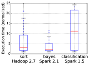
(a) Execution time

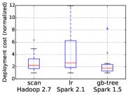
(b) Deployment cost

Figure 3: The execution time and deployment cost of workloads running on 18 virtual machines (different types). The execution time of classification-Spark 1.5 using worst VM type is 20 times slower that the best VM type. Similarly the deployment cost of running Linear Regression the worst VM type is 10 times more expensive than the best VM type.

No VM rules all: Our empirical data, as shown in Figure 3, demonstrates that a bad choice can increase the execution time (of a workload) up to 20 times and can be ten times more costly than the optimal one. Prior work reports similar results [4, 1]. Careless selection can often end up with high deployment cost and longer (sub-optimal) execution time.

Even though users are willing to pay a higher cost in exchange for performance, choosing the most expensive VM type may not always result in optimal performance. Figure 4(a) shows the distribution of the execution time when running on the most expensive VM types (namely c4.2xlarge, m4.2xlarge and r4.2xlarge). For instance, if we look at the distribution of execution times for c4.2xlarge, we observe that c4.2xlarge is the best VM for 50% of the cases. This means for the other 50% of the workloads; the most expensive VM type does not guarantee the lowest execution time. We observe similar behavior in Figure 4(b), where the least expensive VM, c4.large, does not ensure the lowest deployment cost.

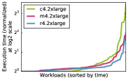
(a) Execution time on the most expensive VM types.

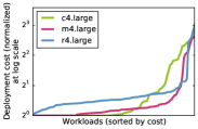
(b) Deployment cost on the least expensive VM types.

Figure 4: Performance distribution over different workloads. The performance is normalized to the optimal performance measured in the 18 virtual machine. The x-axis represents workloads, sorted by their normalized performance. Both choosing the most expensive and the cheapest VM types are not desirable.

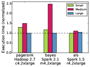
(a) Execution time.

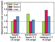
(b) Deployment cost.

Figure 5: Running application with different input sizes result in very different performance. The best performing VM types for an application can change when the input size or parameters are changed.

The same application with different input sizes favors different VM types: Machine learning workloads are readily available such as the machine learning library in Apache Spark and Python [18]. It is valid to assume that similar workloads would prefer the same VM type provided the user can accurately identify similar workloads. Consequently, users can always reuse the best VM type for their workloads without testing further. However, we found that this might not always be the case. A workload with different input sizes or parameters performs very differently on different VMs [19]. Figure 5 illustrates how the performance of an application varies with different input sizes. For example, in Figure 5(b) m4.2xlarge is the most cost-effective VM type for running the bayes application with the small input size. However, the deployment cost increases by 40% (is no longer the optimal VM) when the input size is large. A possible explanation is that a larger input size creates a resource bottleneck on a smaller VM. Hence, users need to be more careful at selecting the best VM type even for similar workloads.

Cost creates a level playing field: Finding a cost-effective VM type can be harder because a slower VM can be competitive in deployment cost. In Figure 4(a), c4.2xlarge is the fastest VM type for over 50% of the workloads (optimal execution time is 1.0). However in Figure 4(b), when considering deployment cost, we observe that c4.large is likely to be a better choice, since it is optimal VM in over 50% of the workloads.

Figure 6 presents the normalized execution time and deployment cost of a workload (regression on Spark 1.5). The figure demonstrates how execution time can be very different while deployment cost is similar across all VM types. For example, m4.2xlarge and r4.xlarge are comparable to c4.2xlarge. When the difference between execution times of a workload in different VM types is large, choosing the best VM is easier because there is a clear winner. Incorporating cost compresses the difference. Therefore, searching for the most cost-effective VM type becomes more difficult because several inferior choices (in terms of execution time) are now competitive (in deployment cost). In Section V-B, we show why finding cost-effective VM type is harder than execution time.

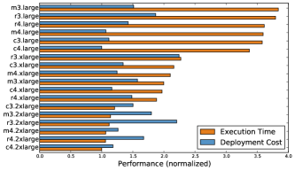
Figure 6: The performance of running the regression workload on instances with different VM types. Introducing cost creates a level playing filed, in which several inferior VM types in execution time are now competitive in deployment cost. This observation implies that searching for the most cost-effective configuration is harder than searching for the fastest configuration.

II-D Search-based optimization instead of complex models

One way to choose the best VM for a given workload is to build a complex prediction model from measurements as done in [1]. However, this approach may encounter several obstacles. First, the method assumes that data collection is free of noise. However, this is not true in a cloud environment due to the sharing infrastructure, and therefore, performance interference is unavoidable [12]. Second, a large amount of training data is required for building such complex models—which is not viable since each execution is expensive. Moreover, even with the availability of data, performance predictability remains an issue. For instance, PARIS shows up to $50\%$ RMSE (Root Mean Squared Error) while predicting performance.

Sequential model-based optimization (SMBO) iteratively measures solutions (VM types) to optimize for an objective (execution time or deployment cost) [9]. SMBO is naturally applicable to finding the best VM. A typical SMBO algorithm is described in Algorithm 1. An SMBO algorithm requires 4 inputs namely, a cloud set up to run a workload ($f$), list of VM characteristics ($vm\in\mathit{VM}$) or instance space, an acquisition function ($S$), and a choice of surrogate model ($M$). SMBO starts with an initial sample of VMs (chosen randomly), which are then measured ($D$). Line 1. SMBO builds a surrogate or a machine learning model to estimate to predict workload performance. This model is constructed using VM characteristics and the measured performance. Line 2. A VM is selected based on the surrogate model along with a predefined acquisition function (see SectionIII-A). Line 4. The selected VM ($x_{i}$) is then measured ($f$). Line 5. The VM ($x_{i}$) along with performance ($y_{i}$) is then added to the already measured VMs ($D=\{(vm_{1},y_{1}),(vm_{2},y_{2})\}$). Line 6. This process terminates after a stopping criterion is reached.

We prefer SMBO because it is resistant to the shortcomings in the complex-model building method, and is suitable for optimizing any expensive black-box function.

Input: $f$, $\mathit{VM}$, $S$, $M$

Output: The optimal configuration

1 $D$ := Initial sampling ($f$, $\mathit{VM}$)

2

3for $k$ in $|\mathit{VM}\notin D|$ do

4       $p(y|vm,D)$ := fit a surrogate model (M, D)

5       $vm_{k}$ := $argmax_{vm\in\mathit{VM}}S(vm,p(y|vm,D))$

6       $y_{k}$ := $f(vm_{k})$

7       $D$ := $D\cup(vm_{k},y_{k})$

8      

9 end for

Algorithm 1 Sequential Model-Based Optimization

III Is Bayesian Optimization Fragile?

In this section, we introduce Bayesian Optimization and explain why BO can be fragile in our problem setting.

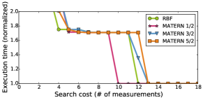
(a) Minimizing execution time for als

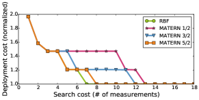
(b) Minimizing deployment cost for bayes

Figure 7: The number of actual measurements required to find the optimal VM type by Bayesian Optimization with different kernel functions. Each kernel function is tested with 100 different sets of initial points uniformly selected. The line represents the median performance from 100 runs.

III-A What is Bayesian Optimization?

BO follows the same formalism of sequential model-based optimization (SMBO) (as described in Section II-D). Like SMBO, BO has two essential components namely a (probabilistic) regression model, and an acquisition function (Refer to [20] for more details.) BO has been used as a drop-in replacement to standard techniques such as random search, grid search and manual tuning in numerous domains such as hyperparameter tuning and software performance optimization [9, 21, 22, 23]. Recently, CherryPick used BO to find the best VM for a specific workload [4].

In BO, Gaussian Process is the standard probabilistic model used for building the surrogate model. Gaussian Process is a distribution over objective functions specified by a mean function and covariance function. Once a surrogate model is trained, it can be used to estimate performance (of a workload) on the unmeasured VM. The surrogate model returns distribution of the estimated performance associated with the VM (mean and variance). The next VM to measure is determined by an acquisition function. Common acquisition functions are Probability of Improvement (PI), Expected Improvement (EI), and Gaussian Process Upper Confidence Bound (GP-UCB) [10]. Recently, the entropy search methods, backed by information theory, are promising alternatives [24]. In practice, EI is effective and used in CherryPick.

An important component in Gaussian Process is the covariance kernel function, which is crucial for model effectiveness. Covariance kernel ensures that the prior, required for GP to be effective, is met. GP assumes smoothness, or in other words, the VMs which are closer to each other in instance space have similar performance. This is particularly difficult in our problem setting, where a slight difference in the instance space and lead to significant differences in performance (cost or time). This goes to show that before using BO (with GP as a surrogate model), a practitioner needs to choose a kernel function to ensure smoothness in the instance space. Aforementioned could be particularly challenging and can affect the performance of BO. CherryPick chooses the Matérn 5/2 kernel function because it does not require strong smoothness, which are the cases for many real-world applications [4, 1].

III-B How to choose the right covariance kernel function?

Since the choosing the covariance kernel function is critical, this section examines how different kernel function can affect the usefulness of BO. We implement a BO (as prescribed by CherryPick) to examine four different kernel functions: (1) RBF: Radial Basis Function is a widely used kernel. However, RBF considers the effects of features on the covariance equally [7], which may not be realistic. Matérn kernel function is another family of covariance functions which incorporates a smoothness parameter such that it is flexible to model different objective functions. The smoothness parameter serves as similarity function that determines whether two samples are alike. The most commonly used smoothness parameters have three kinds namely, (2) Matérn 1/2, (3) Matérn 3/2, and (4) Matérn 5/2.

Figure 7 shows the number of actual measurements required to find the best VM for a given workload. In Figure 7(a), shows how BO with Matérn 1/2 kernel can find the optimal VM faster thereby reducing the search cost. However, in Figure 7(b), while trying to find a cost-effective VM, BO with Matérn 1/2 kernel performs the worst. The two particular examples we want to demonstrate how choosing the appropriate kernel function affects the performance of BO. In practice, choosing the right kernel function relies on engineering and automatic model selection [7, 8, 9, 10].

Our prior experience [5] indicates that it is possible to have non-smooth performance outcome for a given workload on different VMs. When a workload hits a resource bottleneck, e.g., memory or disk, it can slow down greatly. This means that a workload might perform very differently on two VMs which are close to each other in the instance space. Therefore, we doubt that architecture parameters along are not sufficient to predict the performance of cloud applications [1, 5].

III-C No one-size-fits-all initial points!

The choice of initial VMs also affects the effectiveness of BO. A common approach is a quasi-random method which uniformly selects very distinct VMs [25]. This method helps capture workload behavior, which can then be used to choose the next best VM to measure. However, in practice, we have seen that BO is sensitive to initial points (VMs in our setting) and can exhibit large variances in their outcome.

To demonstrate the effect of initial VMs on the performance of BO, we choose three very different starting points, i.e., c4.xlarge, m4.large and r3.2xlarge, and then run BO on all the 107 workloads. We observe that about 15% applications do not find the optimal configuration within six attempts (33% of the instance space). We then redo the same experiment but choose different initial VMs. We find that the BO can find the optimal configuration within six attempts. This result demonstrates that the initial points dramatically affects the performance of BO.

Even though there exists a set of initial points that work well on almost all applications, the optimal initial VMs are subject to change because new VMs are frequently added to the Cloud portfolios. Therefore, it is essential to design a search method that performs consistently with different initial points.

III-D Summary

BO is a promising technique for finding the best VM for any workload. However, our large-scale evaluation shows that a BO method can be fragile or unstable. Without proper design, it may lead to high search cost or a sub-optimal solution. This is because the effectiveness of BO is significantly affected by choice of the kernel function and the initial VMs (used to seed the BO). However, choosing the suitable kernel function requires further analysis and in-depth study. To sum up, BO can be fragile and requires extra care while making design choices. Our objective is to attempt to make BO less fragile by (i) augmenting BO with additional (low-level) information and (ii) use variants of BO - which are less sensitive.

IV Low-Level Insight

In this section, we introduce how to leverage low-level performance information to augment Bayesian Optimization.

IV-A Choosing the Low-Level Metrics

Prior work has shown how low-level performance metrics of workload are information, which is a good proxy for predicting performance [12, 5, 17, 1]. For example, the memory commit size represents the amount of memory required to handle current workload, and the CPU time waiting on I/O indicates the workload type or a bottleneck on I/O. However, in practical settings, we need to analyze multiple metrics to better understand the factors which affect performance. System utilities on Linux, such as sysstat, provides a comprehensive set of performance metrics [26], which are useful to characterize workloads and identify performance bottlenecks. In this work, we use these low-level metrics to augment a BO. The intuition behind this design choice stems from the fact that only instance space (published VM characteristics) is inadequate to fully characterize a VM. In Figure 8, we show an example to use the low-level information to to identify the memory bottleneck while running Logistic Regression.

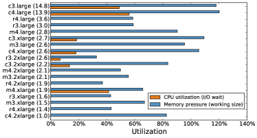
Figure 8: A memory bottleneck is identified by low-level performance information. The horizontal axis represents the resource utilization (%), and the vertical axis represents the VM types. The numbers in the parenthesis are the normalized execution time where 1.0 represent the best VM type. The memory of a small VM type (c3.large) is not sufficient to run Logistic Regression, which leads to 14.8 times slower than the best VM type (c4.2xlarge). This behavior is captured by memory pressure and CPU utilization.

Since we focus on recurring jobs, we should use metrics that can capture the workload progress and identify resource bottleneck. The selection of low-level metrics depends heavily on workloads. If possible, we should use a comprehensive set of metrics. However, a large number of features can lead to the over-fitting problem in building predictive models. This is known as the curse of dimensionality [27]. In this work, we find the following low-level metrics are effective. Automatic feature selection can help address this problem [28, 5] but will require further studies.

• Workload progress: CPU utilization on user time, I/O wait time, and the number of tasks in the task list.

• Memory pressure: % of commits in memory.

• I/O pressure: disk utilization and wait time (disk).

IV-B Low-Level Augmented Bayesian Optimization

Leveraging low-level information in BO requires novel modeling methods because the given workload is yet to be executed on the candidate VM. Our approach, instead, predicts the performance (cost or time) based on the VM characteristics and observed low-level metrics of the VM that is already measured. This is similar to the reasoning technique used in practical settings by experts and the table based models [29]. Experts choose to interpolate or extrapolate the workload performance using not only characteristics of VM but also the low-level performance information.

We make the following design choices to modify Naive BO to integrate low-level performance information into BO:

Augmented Instance Space: Instead of using only VM characteristics ($\mathit{VM}_{i}$), as an input to the surrogate model we also use low-level metrics ($L_{i}$) collected from running the workload on ($\mathit{VM}_{i}$). These constitute the independent variables. Similar to Naive BO, the performance of the workload is used as the dependent variable. Decision to use low-level information allows BO to make more informed search.

Surrogate Model: Instead of using Gaussian Process as the surrogate model, we choose a tree-based ensemble method Extra-Trees algorithm for building the surrogate model. The tree-based learning method is effective to capture complex performance behavior  [30, 31, 32, 5, 1]. We choose not to use Gaussian Process in Bayesian Optimization because determining the right kernel function (as discussed in Section III-B) requires careful evaluation, which is not practical for supporting diverse workloads. This design choice lets us side-step one of the reasons for the fragility of Naive BO.

Acquisition Function: We replace Expected Improvement (EI) with Prediction Delta as the acquisition function. Prediction delta can select a VM type with highest estimated performance (least execution time or cheapest deployment cost). Prediction Delta can also be used as a stopping criterion—terminate the search process if there exists no better VM type. We do not use Expected Improvement as our acquisition function because it is not useful when the kernel function cannot estimate the black-box function. This design choice for an acquisition function which does not require a suitable kernel function.

Surrogate Model Update: When updating the surrogate model upon a new observation for workload (w) ($\mathit{VM}_{i,w}$, $L_{i,w}$ and $y_{i,w}$), we generate multiple pairs of input ($\mathit{VM}_{j,w}$, $\mathit{VM}_{i,w}$), where $i\neq j$ with low-level information ($L_{j,w}$), where $j$ represent the source VM—which has been measured and $i$ represents the destination VM—which is yet to be measured. This surrogate model answers “what is the predicted performance of $\mathit{VM}_{i,w}$ given the low-level performance information observed on a particular VM ($\mathit{VM}_{j,w}$)”. For example, if we have measured the performance of workload (w) in 3 VMs ($VM_{1,w},VM_{2,w},VM_{3,w}$), the number of independent values for which the performance needs to be estimated would be $3\times(18-3)$. It should be noted that to estimate the performance of a workload in a VM (say $\mathit{VM}_{15,w}$), requires considering $\mathit{VM}_{1,w}\rightarrow\mathit{VM}_{15,w}$, $\mathit{VM}_{2,w}\rightarrow\mathit{VM}_{15,w}$, and $\mathit{VM}_{3,w}\rightarrow\mathit{VM}_{15,w}$. Since multiple pairs exist, we average the estimated performance. This design choice helps us update the surrogate model even when the low-level information of destination VM is not available.

Algorithm 2 illustrates the Augmented BO.

Input: $f$, $\mathit{VM}$, $S$, $M$

Output: The optimal configuration

1 $D$ := Initial sampling ($f$, $\mathit{VM}$)

2

3for $k$ in $|\mathit{VM}\notin D|$ do

4       $p(y|vm,D,L)$ := FitLowLevelModel(M, D, L)

5       $vm_{k}$ := $argmax_{vm\in\mathit{VM}}S(x,p(y|vm,L,D))$

6       $y_{k},L_{k}$ := $f(\mathit{vm}_{k})$

7       $D$ := $D\cup(\mathit{vm}_{k},y_{k},L_{k})$

8      

9 end for

Algorithm 2 Low-Level Augmented Bayesian Optimization (similar to Algorithm 1)

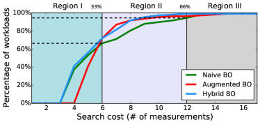
(a) Optimizing running time

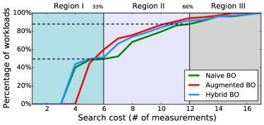
(b) Optimizing running cost

Figure 9: Search cost of finding the optimal VM type across the 107 workloads. The y-axis represents the cumulative percentages of workloads. In Region I, although Augmented BO does not find the optimal VM type at the fourth step, it does find a very near optimal solution with only 4% difference. Section VI provides further details.

V Evaluation

This section describes our experimental setting and evaluation method to compare Augmented BO with Naive BO.

V-A Experimental Method

Workload: For evaluation, we use Apache Hadoop (v2.7) and Spark (v2.1 and v1.5), which are popular systems for many big data and machine learning applications. We choose distinct workloads from HiBench and spark-perf, as listed in Table I. HiBench is a big data benchmark suite for Apache Hadoop and Spark [33]. It was designed to test batch processing jobs and streaming workloads. Similarly, spark-perf is a performance testing suite for Spark [34]. The testing suite provides a wide range of workloads including supervised learning such as regression and classification modeling, unsupervised learning such as K-Means clustering, and statistical tools such as correlation analysis, and Principal Component Analysis (PCA). We run 107 workloads to test their performance on 18 VM types. During the execution of the workload, a sysstat demon is run in the background to collect low-level performance information [26]. We do not find any signification overhead to collect low-level information.

Cloud Configurations: We measure the performance on six VM families (available on AWS) {c3, c4, m3, m4, r3 and r4}, and three VM sizes {large, xlarge and 2xlarge}. The VM size represents the core count. For example, c4.large has two cores, c4.xlarge has four cores and c4.2xlarge has eight cores.

Encode Cloud Configurations: We choose four VM characteristics namely CPU types, core count, average RAM per core, and the bandwidth to Elastic Block Storage (EBS). We encode the four features with numerical values into $\vec{\mathit{VM}}$. The CPU types are encoded from one to six in order, and for the core count, we use their actual values {2, 4, 8}. Similarly, the RAM size per core is {2, 4, 8}. Last, the bandwidth to EBS has three classes for different VM types encoded as {1, 2, 3}.

V-B Comparison

This section evaluates Naive BO and Augmented BO, on the 107 workloads with randomly selected initial VMs. The above process is repeated 100 times to account for randomness. Here we minimize execution time and deployment cost individually. Figure 9 presents the overall result.

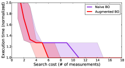
(a) PageRank on Hadoop 2.7

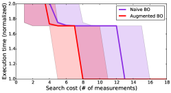
(b) Alternating Least Squares on Spark 2.1

(c) Logistic Regression on Spark 1.5

Figure 10: Examples of searching for the best VM. The objective is to find the fastest VM in subfigures (a, b) and the most cost-effective VM in subfigure (c). Both the BO methods stops after they find the optimal VM type (normalized to 1.0). The line represents the median value of the execution time over 100 repeats. Each repeat used different initial points to seed BO. The shaded region represents the IQR or Interquartile range is the difference between $3^{rd}$ and $1^{st}$ quartile. A high value (larger area) of IQR indicates high variance.

RQ1: Can Augmented BO find optimal VMs?

Figure 9(a) shows the percentage of workloads, where Naive BO and Augmented BO found the optimal VM. The horizontal axis represents the search cost (in terms of # of measurements), and the vertical axis represents the percentage of the workloads. In this figure the green line represent the Naive BO and the red line represent the Augmented BO. The Naive BO can find the optimal solution for 60% of the workloads by searching 33% of the search space (Region I). The performance of Augmented BO is similar to naive BO. However, Augmented BO has a slow start problem but becomes effective eventually. In Region II, Augmented BO is a clear winner as it can find optimal VMs for 96% of the workloads within ten measurements. At the same time, Naive BO can only find 80% of the workload.

We claim that the performance of Augmented BO is better than Naive BO, for regions I and II (at step 6 and 12). We also observe an interesting phenomenon—Augmented BO is outperformed by Naive BO in initial four steps. The one-step difference can be attributed to the over-fitting problem caused by the larger training features (both high-level and low-level information) in Augmented BO. This is a challenge of leveraging low-level information (for future work).

While looking at the performance of VMs selected by Augmented BO, we observe that the best VM found by Augmented BO is only 4% away from the optimal VM. In practice, this difference can be easily ignored (refer to Section VI). Furthermore, with the growing instance space, this difference (though we believe is little) can be amortized because the search cost will also increase.

A possible workaround to this problem can be to create a Hybrid BO (shown in blue)—which combines the best of the two methods. Figure 9(a) shows that Hybrid BO outperforms Naive BO for in all cases. However, we choose not to focus on the hybrid method in this paper because of space constraints. Another reason why we do not discuss Hybrid BO because our primary objective is to identify the fragility of Naive BO and the advantages of leveraging low-level information.

RQ2: Can Augmented BO minimize cost?

To answer the question if Augmented BO can minimize the deployment cost, it is essential to demonstrate that Augmented BO can find optimal VM faster than Naive BO (lower search cost). In Figure 9(b), we observe that the minimizing deployment cost is more difficult i.e., both methods require more search cost to reach the optimal solution. We observe that Naive BO can find the best VM with six attempts for only 50% applications while Augmented BO increases this probability to 60%. We also see a clear win for Augmented BO as it can find best VM which minimizes the deployment cost after measuring five measurements. However, we see that Augmented suffers from a slow start, which is similar to Figure 9(a) and Hybrid BO (shown in blue) is the workaround.

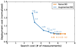
(a) Region I

(b) Region II

(c) Region III

Figure 11: Comparison between effectiveness of search with different stopping criteria. There is a trade-off between search cost and deployment cost. In Region I, Augmented BO is comparable with Naive BO in terms of deployment cost but can greatly reduce search cost at the expense of slight increase in deploymwnr cost. For Region II and Region III, Augmented BO outperform Naive BO for both search cost and deployment cost.

RQ3: Is Augmented BO fragile?

In finding the best VM, Naive BO fails in 36% (minimizing time) and 50% (minimizing cost) of the workloads after measuring the performance of the six VMs (Region I). Augmented BO alleviates this problem, and this can be observed by a up to 20% increase in the number of workloads for which Augment BO found the optimal VM (step 7 in Figure 9(b)).

Stability is another important aspect of Augmented BO. As discussed in Section III-C, initial points are critical to the performance of BO—different initial VMs can lead to very different results (performance and search cost) or high variances in results. Figure 10 compares the search cost and the performance found by the two methods. We present the median value (shown by line), and the interquartile range (the difference between the $3^{rd}$ and the $1^{st}$ quartile) shown by the shaded region. The three cases show that Augmented BO yields less search cost and reduces the variance. This demonstrates Augmented BO is not fragile.

Another interesting observation is that Augmented BO not only alleviates the fragile problem in Region II but also moves workloads from Region III to Region II.  Figure 10(a) and  Figure 10(b) are example workloads in Region III. The first quartile indicates that Augmented BO finds the optimal configuration even with four or five attempts in 25% initial points that are tested.

VI Practical Implications

VI-A Bayesian Optimization in Practice

In practice, users can tolerate a loss in performance (deployment cost or execution time) in exchange for lower search cost. In this section, we examine the performance of the two methods when we (slightly) relax the definition of optimality. Due to space limitations, we only present the results of minimizing deployment cost as we have shown it is more challenging, and the conclusion is similar to minimizing execution time.

To demonstrate the performance (of BO) and search cost trade-off, we vary the stopping criteria to understand how they affect both search cost and the best VM they find. We choose EI as the stopping criteria for Naive BO (as prescribed by CherryPick). For Augmented BO, we use Prediction Delta and vary the thresholds from 0.9 to 1.3. We examine the three regions separately to analyze the effects of stopping criterion on different categories of workload.

In Figure 11(a), Naive BO finds the optimal VM regardless of the stopping criteria. This is counter-intuitive because there should exist a trade-off between the deployment cost and the search cost. We hypothesize that Naive BO cannot estimate that it has found the optimal VM. Augmented BO, on the other hand, clearly shows the trade-off. Augmented BO with the thresholds $1.25$ and $1.3$ performs similarly to Naive BO. As pragmatic engineers, we are always hard-pressed to recommend Naive BO over Augmented BO, which achieves a performance of 1.04 rather than a perfect 1.0.

In Figures 11(b) and 11(c), Augmented BO is the clear winner. With the $1.1$ threshold, Augmented BO outperforms Naive BO in both the search cost and the deployment cost. To simplify the comparison, we choose 10% EI for Naive BO (as prescribed by CherryPick) and 1.1 threshold for Augmented BO. Our method yields lower search cost while achieving lower deployment cost. On average, it finds VMs which 5% lower in deployment cost while reducing search cost by 20%. This demonstrates that the low-level augmented Bayesian Optimization finds the well-suited VMs quicker and is more precise when compared to Naive BO.

Overall, we recommend using $1.1$ threshold in Augmented BO since the deployment cost is comparable with Naive BO and reduces the search cost. In Figure 12, we present the overall comparison of the two methods with the EI and threshold described above. The horizontal axis represents the reduction in search cost, and the vertical axis represents the decrease in the deployment cost (higher the better in both). The figure shows the result for all 107 workloads represented as points. Points enclosed with lines $x=0$ and $y=0$ (shown in blue shade) indicates workloads, where Augmented BO can find VMs which have lower deployment cost using lower search cost. For example, the workload represented in (24, 10) is the case where Augmented BO uses 24% lower search cost, and the best VM found (for that workload) has 10% lower deployment cost than the one found by Naive BO. There are 46 such workloads. Augmented BO requires higher search cost than Naive BO in five workloads (region shaded in red). But they both find the optimal solution. There are 17 workloads where Augmented BO finds VM types with higher running cost but with lower search cost—a region of trade-off.

VI-B Time-Cost Trade-off

This section demonstrates how to adapt Augmented BO as well as Naive BO to navigate the time-cost trade-off. In practice, a user would always want a solution to reduce time as well as cost. We propose a new measure called time-cost product which is similar to an energy-time trade-off in high-performance computing [35]. Not every time-cost trade-off is desirable because a small improvement in performance may incur a higher running cost. For example, a 10% improvement in execution time requires a 50% increase in deployment cost.

For simplicity, we assign the same importance to time and cost. That is, it is considered desirable for a 10% improvement in time and a 10% increase in cost. To support the time-cost trade-off, instead of predicting the execution time and deployment cost, the surrogate model estimates the product of time and cost. Any two VMs are considered the same if their products of execution time and deployment cost are the same. Similarly, a larger product represents an undesirable choice.

Figure 13 presents the comparison which is similar to Figure 12. We observe a great reduction, i.e., $>50\%$ in search cost. Naive BO exhibits long searching process (more than six attempts) in 24 percent workloads and very long searching (at least ten attempts) in 13 percent workloads. On the other hand, Augmented BO requires no more than 6 actual evaluation for all 107 applications. Please note that the threshold used for this experiment is 1.05, which also tells us that the stopping criteria also need to be changed based on the workload as well as the performance objective.

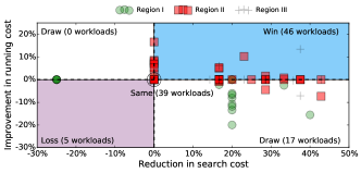
Figure 12: Overall comparison for the two BO methods in finding the most cost-effective VM type across the evaluated 107 workloads. The numbers are calculated as the reduction percentage in search cost and improvement in deployment cost, both higher the better. Workloads in (0,0) represent workload which achieve similar performance in both methods.

VII Related Work

State-of-the-art: Ernest exploits the internal structure of a workload to predict performance when running in different cluster sizes. This greatly reduces the search cost because a workload can be experimentally tested on a smaller cluster. CherryPick implements an optimization engine that uses Bayesian Optimization in searching for the best configuration [4]. However, CherryPick does not leverage low-level information and uses Gaussian Process-based BO, which makes it fragile. PARIS shares the same goal with our work [1]. It builds a comprehensive performance model from the large training dataset and uses it along with current measurements However, we argue that such approach might not be suitable for batch processing workloads because of the low prediction accuracy as discussed in Section II-D.

System Performance tuning: BOAT is a structured Bayesian Optimization-based framework for automatically tuning system performance  [6] which leverages contextual information. BOAT combines the parametric and non-parametric model for better predicting the trend in system performance. The idea behind their work and our work is very similar: leveraging domain knowledge to enhance BO.

Bilal et al. propose a framework to automate tuning system performance of stream-processing systems.Their modified hill-climbing search with heuristic sampling inspired by Latin Hypercube improves the search process by two to five times. Several papers use minimal sampling techniques to build models to optimize software systems [36], [37, 22, 38]. The above methods reduce the search cost by a significant degree. However, they focus on performance tuning for the same workload (or application) on the same type of machine. It is not clear how to leverage their approaches to support different machine configurations in cloud computing. We, instead, find the best machine configuration for a given workload.

Leveraging low-level performance: Low-level performance information is leveraged to identify performance bottlenecks and to predict application performance. DeepDive is designed to identify performance interference of co-existing VMs  [12]. Wang et al. propose using the CART model to predict storage performance. Their approach requires workload information, which may not be practical for our problem setting. Inside-out provides reliable performance prediction of distributed storage service by using only low-level performance information [5]. The authors show that high-level performance can be accurately captured by only the low-level metrics. This accurate prediction model can be used to adjust resource allocation for meeting performance objectives.

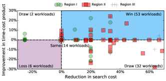
Figure 13: Similar to Figure 12, the optimization objective is to find the best configuration both in execution time and search cost. Augmented BO supports finding the best VM type, given a time-cost tradeoff.

VIII Conclusion

In this paper, we identify and demonstrate the fragility of Bayesian Optimization in finding the best cloud VM type. The fragility arises from the inadequate information used to represent the instance space. This fragility affects prior work which uses only instance space to guide Bayesian Optimization. To overcome the problem of fragility, we augment the instance space with low-level performance information, which is known to be useful for characterizing the performance of the system. We present our method, Augmented Bayesian Optimization, which seamlessly integrates the low-level metrics (obtained with negligible overhead) to the surrogate model. Additionally, we make design choices to modify existing BO to make more informed decisions. We demonstrate empirically the usefulness of Augmented BO by showing that Augmented BO can find the best VM type across all workloads. In 46 out of 107 workloads, Augmented BO outperforms the state-of-the-art Bayesian optimization method in terms of both performance and search-cost.

More generally, we conclude that it is often insufficient to use general-purpose off-the-shelf methods (BO in this case) for selecting the best VM without augmenting those methods with essential systems knowledge such as CPU utilization, working memory size and I/O wait time. In our future work, we plan to further augment Bayesian Optimizer with historical performance data to further reduce the search cost.

References

- [1] N. J. Yadwadkar, B. Hariharan, J. E. Gonzalez, B. Smith, and R. Katz, “Selecting the Best VM across Multiple Public Clouds : A Data-Driven Performance Modeling Approach,” in ACM Symposium on Cloud Computing 2017 (SoCC’17), 2017.
- [2] S. Frey, F. Fittkau, and W. Hasselbring, “Search-based genetic optimization for deployment and reconfiguration of software in the cloud,” in The 2013 International Conference on Software Engineering (ICSE’13). IEEE Press, 2013, pp. 512–521.
- [3] Y. Yao, Z. Xiao, B. Wang, B. Viswanath, H. Zheng, and B. Y. Zhao, “Complexity vs. Performance: Empirical Analysis of Machine Learning as a Service,” in The 2017 Internet Measurement Conference (IMC ’17), vol. 1417, 2017, pp. 384–397.
- [4] O. Alipourfard, H. H. Liu, J. Chen, S. Venkataraman, M. Yu, and M. Zhang, “CherryPick : Adaptively Unearthing the Best Cloud Configurations for Big Data Analytics,” in 14th USENIX Symposium on Networked Systems Design and Implementation (NSDI 17), 2017, pp. 469–482.
- [5] C.-J. Hsu, R. K. Panta, M.-r. Ra, and V. W. Freeh, “Inside-Out : Reliable Performance Prediction for Distributed Storage Systems in the Cloud,” in The 2016 IEEE 35th Symposium on Reliable Distributed Systems (SRDS 2016), 2016, pp. 127–136.
- [6] V. Dalibard, M. Schaarschmidt, and E. Yoneki, “BOAT: Building Auto-Tuners with Structured Bayesian Optimization,” in The 26th International Conference on World Wide Web (WWW ’17), 2017, pp. 479–488.
- [7] E. Brochu, V. M. Cora, and N. De Freitas, “A tutorial on Bayesian optimization of expensive cost functions, with application to active user modeling and hierarchical reinforcement learning,” ArXiv, p. 49, 2010.
- [8] J. Snoek, H. Larochelle, and R. P. Adams, “Practical Bayesian Optimization of Machine Learning Algorithms,” in Advances in Neural Information Processing Systems 25 (NIPS 2012), F. Pereira, C. J. C. Burges, L. Bottou, and K. Q. Weinberger, Eds. Curran Associates, Inc., 2012, pp. 2951–2959.
- [9] I. Dewancker, M. McCourt, and S. Clark, “Bayesian Optimization Primer,” 2015. https://sigopt.com/static/pdf/SigOpt_Bayesian_Optimization_Primer.pdf
- [10] B. Shahriari, K. Swersky, Z. Wang, R. P. Adams, and N. De Freitas, “Taking the human out of the loop: A review of Bayesian optimization,” Proceedings of the IEEE, vol. 104, no. 1, pp. 148–175, 2016.
- [11] P. Bodik, M. Goldszmidt, A. Fox, D. B. Woodard, and H. Andersen, “Fingerprinting the datacenter: automated classification of performance crises,” in The 5th European Conference on Computer Systems (EuroSys’10), 2010, p. 111.
- [12] “DeepDive: Transparently Identifying and Managing Performance Interference in Virtualized Environments,” in The 2013 USENIX Annual Technical Conference (USENIX ATC’13), 2013, pp. 219–230.
- [13] “Amazon web services.” https://aws.amazon.com
- [14] “Apache hadoop.” https://hadoop.apache.org
- [15] “Apache spark.” https://spark.apache.org
- [16] “Aws ec2 document history.” http://docs.aws.amazon.com/AWSEC2/latest/UserGuide/DocumentHistory.html
- [17] K. Ousterhout, C. Canel, S. Ratnasamy, and S. Shenker, “Monotasks: Architecting for Performance Clarity in Data Analytics Frameworks,” 2017, pp. 184–200.
- [18] “scikit-learn.” http://scikit-learn.org
- [19] S. Venkataraman, Z. Yang, M. Franklin, B. Recht, and I. Nsdi, “Ernest : Efficient Performance Prediction for Large-Scale Advanced Analytics This paper is included in the Proceedings of the,” in 13th USENIX Conf. Networked Syst. Des. Implement., 2016, pp. 363–378.
- [20] B. Shahriari, K. Swersky, Z. Wang, R. P. Adams, and N. de Freitas, “Taking the human out of the loop: A review of bayesian optimization,” Proceedings of the IEEE, vol. 104, no. 1, pp. 148–175, 2016.
- [21] D. Golovin, B. Solnik, S. Moitra, G. Kochanski, J. Karro, and D. Sculley, “Google vizier: A service for black-box optimization,” in The 23rd ACM SIGKDD International Conference on Knowledge Discovery and Data Mining (KDD ’17). ACM, 2017, pp. 1487–1495.
- [22] V. Nair, Z. Yu, and T. Menzies, “Flash: A faster optimizer for sbse tasks,” arXiv preprint arXiv:1705.05018, 2017.
- [23] M. Zuluaga, A. Krause, and M. Püschel, “-pal: an active learning approach to the multi-objective optimization problem,” The Journal of Machine Learning Research, vol. 17, no. 1, pp. 3619–3650, 2016.
- [24] Z. Wang and S. Jegelka, “Max-value entropy search for efficient Bayesian optimization,” in Proceedings of the 34th International Conference on Machine Learning, ser. Proceedings of Machine Learning Research, D. Precup and Y. W. Teh, Eds., vol. 70. International Convention Centre, Sydney, Australia: PMLR, 06–11 Aug 2017, pp. 3627–3635. http://proceedings.mlr.press/v70/wang17e.html
- [25] I. M. Sobol, “On quasi-monte carlo integrations,” Mathematics and Computers in Simulation, vol. 47, no. 2, pp. 103–112, 1998.
- [26] “sysstat.” http://sebastien.godard.pagesperso-orange.fr
- [27] P. Domingos, “A few useful things to know about machine learning,” Communications of the ACM, vol. 55, no. 10, pp. 78–87, 2012.
- [28] I. Guyon and A. Elisseeff, “An introduction to variable and feature selection,” Journal of machine learning research, vol. 3, no. Mar, pp. 1157–1182, 2003.
- [29] E. Anderson, “Simple table-based modeling of storage devices,” Technical Report HPL-SSP-2001-04, HP Laboratories, Tech. Rep., 2001.
- [30] “Storage device performance prediction with CART models,” in The 12th IEEE International Symposium on the Modeling, Analysis, and Simulation of Computer and Telecommunication Systems (MASCOTS 2004). IEEE, 2004, pp. 588–595.
- [31] L. Y. L. Yin, S. Uttamchandani, and R. Katz, “An Empirical Exploration of Black-Box Performance Models for Storage Systems,” in The 14th IEEE International Symposium on the Modeling, Analysis, and Simulation of Computer and Telecommunication Systems (MASCOTS 2006). IEEE, 2006, pp. 433–440.
- [32] “Predictive performance modeling of virtualized storage systems using optimized statistical regression techniques,” in The 4th ACM/SPEC International Conference on Performance Engineering (ICPE 2013). ACM Press, apr 2013, p. 283.
- [33] “Hibench.” https://github.com/intel-hadoop/HiBench
- [34] “spark-perf.” https://github.com/databricks/spark-perf
- [35] “Analyzing the energy-time trade-off in high-performance computing applications,” IEEE Transactions on Parallel and Distributed Systems, vol. 18, no. 6, pp. 835–848, 2007.
- [36] V. Nair, T. Menzies, N. Siegmund, and S. Apel, “Using bad learners to find good configurations,” arXiv preprint arXiv:1702.05701, 2017.
- [37] J. Oh, D. Batory, M. Myers, and N. Siegmund, “Finding near-optimal configurations in product lines by random sampling,” in Proceedings of the 2017 11th Joint Meeting on Foundations of Software Engineering. ACM, 2017, pp. 61–71.
- [38] V. Nair, T. Menzies, N. Siegmund, and S. Apel, “Faster discovery of faster system configurations with spectral learning,” arXiv preprint arXiv:1702.05701, 2017.