Kernel Robust Bias-Aware Prediction under Covariate Shift

Abstract

Under covariate shift, training (source) data and testing (target) data differ in input space distribution, but share the same conditional label distribution. This poses a challenging machine learning task. Robust Bias-Aware (RBA) prediction provides the conditional label distribution that is robust to the worst-case logarithmic loss for the target distribution while matching feature expectation constraints from the source distribution. However, employing RBA with insufficient feature constraints may result in high certainty predictions for much of the source data, while leaving too much uncertainty for target data predictions. To overcome this issue, we extend the representer theorem to the RBA setting, enabling minimization of regularized expected target risk by a reweighted kernel expectation under the source distribution. By applying kernel methods, we establish consistency guarantees and demonstrate better performance of the RBA classifier than competing methods on synthetically biased UCI datasets as well as datasets that have natural covariate shift.

Introduction

In standard supervised machine learning, data used to evaluate the generalization error of a classifier is assumed to be independently drawn from the same distribution that generates training samples. This assumption of independent and identically distributed (IID) data is partially violated in the covariate shift setting (?), where the conditional label distribution $P(y|x)$ is shared by source and target data, but the distribution on input variables $P(x)$ differs between source and target samples, i.e., $P_{\text{src}}(x)$ differs from $P_{\text{trg}}(x)$. All models trained under IID assumptions can suffer from covariate shift and provide overly optimistic extrapolation when generalizing to new data (?). An intuitive and traditional method to address covariate shift is by importance weighting (?; ?), which tries to de-bias the objective loss function by weighting each instance with the ratio ${P_{\text{trg}}(x)}/{P_{\text{src}}(x)}$. However, importance weighting not only results in high variance predictions, but also only provides generalization performance guarantees when strong conditions are met by the source and target data distributions (?).

The recently developed robust bias aware (RBA) approach to covariate shift (?) is based on a minimax robust estimation formulation (?) that assumes the worst case conditional label distribution and requires only source feature expectation matching as constraints. The approach provides conservative target predictions when the target distribution does not have sufficient statistical support from the source data. This statistical support is defined by the choice of source statistics or features. The classifier tries to make the prediction certainty under the target distribution as small as possible, but feature matching constraints prevent it from doing so fully. As a result, less restrictive feature constraints produce less certain predictions on target data from the resulting classifier. As shown in Figure 1(a), with limited features, the classifier may allocate most of the certainty under portions of the source distribution (solid line) where the target distribution (dashed line) density is small to satisfy the source feature expectation matching constraints, leaving too much uncertainty in portions of the target distribution. On the other hand, when there are more restrictive features constraining the conditional label distribution, the classifier produces a better model of the data and gives more informative predictions with less target entropy and logloss, as in Figure 1(b). This relation inspires our contribution: leveraging kernel methods to provide higher dimensional features to the RBA classifier without introducing a proportionate computational burden.

According to the representer theorem (?), the minimizer of regularized empirical loss in reproducing kernel Hilbert space can be represented by a linear combination of kernel products evaluated on training data. Model parameters are then obtained by estimating the coefficients of this linear combination. However, in the robust bias-aware classification framework, the objective function of the dual problem is the regularized expected logarithmic loss under the target data distribution. It cannot be computed explicitly using data because labeled target samples are unavailable. Meanwhile, the distribution discrepancy when evaluating the risk function and sampling training data prevents us from applying the representer theorem directly.

(a) First moment features	(b) Third moment features
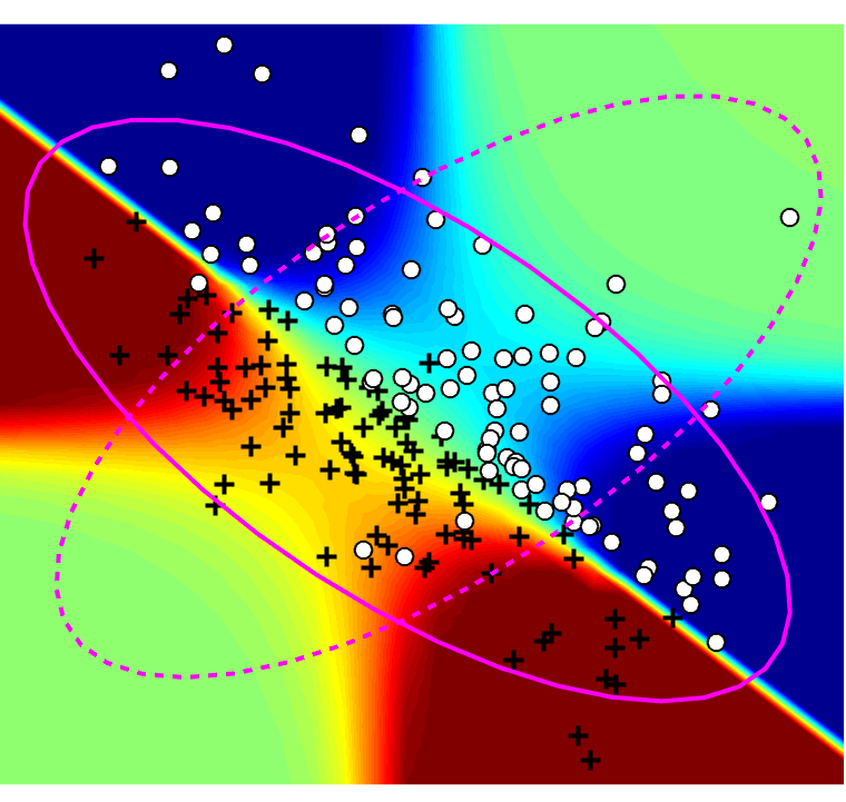
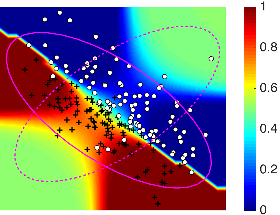
logloss: 0.74	logloss: 0.53
entropy: 0.93	entropy: 0.73

Figure 1: Performance comparison with the robust bias aware classifier using first-order features (a) and first-order through third-order features (b). Labeled source data samples (‘o’ and ‘+’ classes), source (solid line) and target (dashed line) distributions that data are drawn from are shown. The colormap represents the predicted probability, $P(y=$‘+’$|x)$. The intersection of the source distribution and the target distribution is better predicted with third-order features and is much more uncertain when only using first moment features. The corresponding target logloss and entropy are shown.

A quantitative form of the representer theorem has been proposed that holds for the continuous case (?) in which a minimizer over a distribution—rather than discrete samples—is sought. The minimizer of regularized expected risk is represented as the expectation under the same probability distribution instead of a linear combination of the training data. We utilize this result to extend the representer theorem for RBA prediction in the covariate shift setting. We show that the minimizer of the regularized expected target risk can be represented as a reweighted kernel expectation under the source distribution. This enables us to apply kernel methods to the robust bias aware classifier.

In this paper, we explore the theoretical foundation of kernel methods for robust covariate shift prediction. We investigate the underlying effect brought by kernelization and establish consistency properties that are realized by applying kernel methods to RBA prediction. We then demonstrate the empirical advantages of the kernel robust bias aware classifier on synthetically biased benchmark datasets as well as datasets that have natural covariate shift bias.

Related Work

To address the shifts between training and testing input distributions, which is known as covariate shift, existing methods often try to reweight the source samples, denoted $\tilde{P}_{\text{src}}(x)$, to make them more representative of target distribution samples. The theoretical argument supporting this approach (?) is that reweighting is asymptotically optimal for minimizing target distribution log loss (equivalently, maximizing target distribution log-likelihood):

$$\mathbb{E}_{P_{\text{trg}}(x)P(y|x)}[\text{loss}(\hat{P}(Y|X),Y)]=$$

$$\lim_{n\rightarrow\infty}\mathbb{E}_{\tilde{P}_{\text{src}}(x)\tilde{P}(y|x)}\left[\frac{P_{\text{trg}}(X)}{P_{\text{src}}(X)}\text{loss}(\hat{P}(Y|X),Y)\right],$$ (1)

where we use $\hat{P}(y|x)$ to represent the estimated predictor and $\tilde{P}(y|x)$ is the empirical distribution.

Most existing covariate shift research follows this idea of seeking an unbiased estimator of target risk (?). Significant attention has been paid to estimating the density ratio ${P_{\text{trg}}(x)}/{P_{\text{src}}(x)}$, which strongly impacts predictive performance (?; ?). Direct estimation methods estimate the density ratio by minimizing information theoretical criterion like KL-divergence (?; ?; ?) or matching kernel means (?; ?) rather than estimating the ratio’s numerator and denominator densities separately. Other methods (?) consider the ratio as an inner parameter within the model and relate the ratio with model misspecification. There are also methods for specific models of the covariate shift mechanism (?; ?). Additional methods have also been recently proposed to address some of the limitations of importance weighting (?).

Theoretical analyses have uncovered the brittleness of importance weighting for covariate shift by analyzing its statistical learning bounds (?; ?). Cortes et al. (?) establish generalization bounds for learning importance weighting under covariate shift that only hold when the second moment of sampled importance weights is bounded, $\mathbb{E}_{P_{\text{src}}(x)}[(P_{\text{trg}}(X)/P_{\text{src}}(X))^{2}]<\infty$. When not bounded, a small number of data points with large importance weights can dominate the reweighted loss, resulting in high variance predictions.

Kernel methods have been employed for estimating the density ratio in importance weighting methods; for example, kernel mean matching (?; ?). uses the core idea that the kernel mean in a reproducing kernel Hilbert space (RKHS) of the source data should be close to that of the reweighted target data and the optimal density ratio is obtained by minimizing this difference. Kernel methods have also served as a bridge between the source and the target domains in broader transfer learning or domain adaptation problems. In these approaches, kernel methods are used to project source data and target data into a latent space where the distance between the two distributions is small or can be minimized (?).

These existing applications of kernel methods for covariate shift are orthogonal to our approach because they are based on empirical risk minimization formulations with the assumption that source data could somehow be transformed to match target distributions. This differs substantially from our robust approach.

Approach

Robust bias-aware classifier

The robust bias-aware classification model is based on a minimax robust estimation framework (2). Under this framework, an estimator player $\hat{P}(Y|X)$ first chooses a conditional label distribution to minimize the logloss and then an adversarial player $\check{P}(Y|X)$ chooses a label distribution from the set ($\Xi$) of statistic-matching conditional probability to maximize the logloss (?):

$$\min_{\hat{P}(Y|X)}\;\max_{\check{P}(Y|X)\in\Xi}\;\text{loss}_{P_{\text{trg}}(X)}\left(\check{P}(Y|X),\hat{P}(Y|X)\right).$$ (2)

Under IID settings, it is known that robust loss minimization is equivalent and dual to empirical risk minimization (?). From this perspective, RBA prediction modifies the dual robust loss minimization problem in contrast to existing importance weighting methods, which modify the primal empirical risk minimization problem. After distinguishing between source and target distributions and using the logarithmic loss, the robust optimization problem reduces to a maximum entropy problem:

$$\!\!\!\max_{\hat{P}(Y|X)}\!H_{P_{\text{trg}}(x)}(Y|X)\triangleq\mathbb{E}_{P_{\text{trg}}(x)\hat{P}(y|x)}[-\!\log\hat{P}(Y|X)]$$ (3)

$$\text{ such that: }\!\hat{P}(Y|X)\!\in\!\Delta\text{ and }\mathbb{E}_{P_{\text{src}}(x)\hat{P}(y|x)}[\Phi(X,Y)]={\bf c},$$

where $\Delta$ defines the conditional probability simplex that $\hat{P}(y|x)$ must reside within, $\Phi$ is a vector-valued feature function that is evaluated on input $x$, and ${\bf c}=\mathbb{E}_{P_{\text{src}}(x,y)}[\Phi(X,Y)]$ is a vector of the expected feature values that corresponds with the feature function, which is approximated using source sample data in practice. Solving for the parametric form of $\hat{P}(y|x)$ from this optimization problem yields:

$$\hat{P}(y|x)={e^{\frac{P_{\text{src}}(x)}{P_{\text{trg}}(x)}\theta\cdot\Phi(x,y)}}\Big{/}{Z(x)},$$ (4)

with a normalization term defined as $Z(x)=\sum_{y^{\prime}\in\mathcal{Y}}\exp\{\frac{P_{\text{src}}(x)}{P_{\text{trg}}(x)}\theta\cdot\Phi(x,y^{\prime})\}$. Minimizing the target logarithmic loss,

$$\theta=\operatornamewithlimits{argmin}_{\theta}\mathbb{E}_{P_{\text{trg}}(x)P(y|x)}[-\log\hat{P}(Y|X)]+\lambda||\theta||^{2}_{2},$$ (5)

provides parameter vector estimates $\theta$. This can be accomplished by approximating the gradient using source samples rather than approximating the objective function (5). After plugging (4) into (5), the gradient using source samples is:

$$\mathbb{E}_{\tilde{P}_{\text{src}}(x)\hat{P}(y|x)}[\Phi(X,Y)]-\tilde{\mathbf{c}}+2\lambda\theta,$$ (6)

with $\tilde{\bf c}\triangleq\mathbb{E}_{\tilde{P}_{\text{src}}(x)\tilde{P}(y|x)}[\Phi(X,Y)]$. Therefore, the RBA approach directly minimizes the expected target logloss rather than approximating it using importance weighting with finite source samples.

As illustrated by Figure 1, the feature function of the RBA predictor $\Phi$ forms the constraints that prevent high levels of uncertainty (entropy) in the target distribution. As a result, more extensive sets of feature constraints may be needed to appropriately constrain the RBA model to provide more certain predictions in portions of the input space where target data is more probable under source distribution, like the intersection of source and target distribution in Figure 1.

Extended representer theorem for RBA

Kernel methods are motivated in the RBA approach to provide a more sufficiently restrictive set of constraints that forces generalization from source data samples to target data. However, the inability to directly apply empirical risk minimization in the RBA approach (5) complicates their incorporation since kernel method applications often use empirical risk minimization as a starting point.

We extend the representer theorem in the RBA approach by first investigating the minimizer of the regularized expected target loss. Theorem  1 shows that the minimizer of a regularized expected target loss can instead be represented by a reweighted expectation under the source distribution. This paves the theoretical foundation of applying kernel methods to RBA, which essentially differs from traditional empirical risk minimization based methods and use expected target loss as a starting point.

(a) Linear	(b) Gaussian	(c) Polynomial-2	(d) Polynomial-3
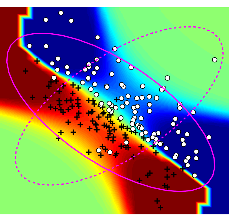
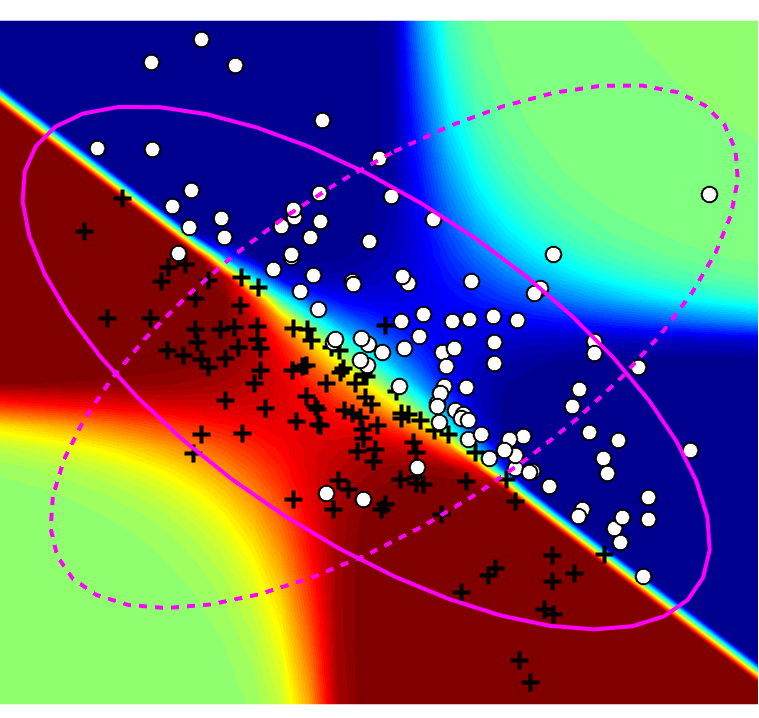
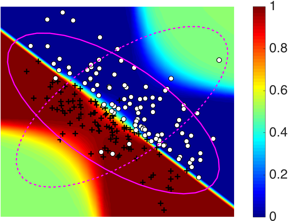
logloss: 0.74	logloss: 0.65	logloss: 0.48	logloss: 0.41
entropy: 0.93	entropy: 0.86	entropy: 0.67	entropy: 0.45

Figure 2: Performance comparison with robust bias aware classifier using linear features (a), using Gaussian kernels with bandwidth 0.5 (b), using polynomial kernels with order 2 (c) and using polynomial kernels with order 3 (d). Ellipses show the same source and target data distribution as in Figure 1. The intersection of source distribution and target distribution is better predicted with kernel methods applied. The corresponding logloss and entropy evaluated on the target distribution shows that more certain and informative predictions are produced by kernel RBA.

Theorem 1.

Let $\mathcal{X}$ be the input space and $\mathcal{Y}$ be the output space, $K$ is a positive definite real valued kernel on $(\mathcal{X},\mathcal{Y})\times(\mathcal{X},\mathcal{Y})$ with corresponding reproducing kernel Hilbert space $H_{k}$, if the training samples $(x_{1}^{s},y_{1}^{s}),\dotsc,(x_{n}^{s},y_{n}^{s})\in\mathcal{X}\times\mathcal{Y}$ are drawn from a source distribution $P_{\text{src}}(x)P(y|x)$ and the testing samples $(x_{1}^{t},y_{1}^{t}),\dotsc,(x_{m}^{t},y_{m}^{t})\in\mathcal{X}\times\mathcal{Y}$ are drawn from a target distribution $P_{\text{trg}}(x)P(y|x)$, any minimizer $f^{*}$ of (5) in $H_{k}$, defining the conditional label distribution,

$$\hat{P}(y|x)={e^{f^{*}(x,y)}}\Big{/}{\sum_{y^{\prime}}e^{f^{*}(x,y^{\prime})}},$$ (7)

admits a representation with a form such that each $f^{*}(x_{i}^{t},y_{i}^{t})=$

$$\frac{P_{\text{src}}(x_{i}^{t})}{P_{\text{trg}}(x_{i}^{t})}\mathbb{E}_{P_{\text{src}}(x)P(y|x)}\left[\alpha(X,Y)K((x_{i}^{t},y_{i}^{t}),(X,Y))\right],$$ (8)

where $\alpha(x_{i},y_{i})\in\mathbb{R}$, for $1\leq i\leq m$, with

$$\theta=\mathbb{E}_{P_{\text{src}}(x)P(y|x)}\left[\alpha(X,Y)\Phi(X,Y)\right].$$ (9)

Proof.

Defining $\Phi^{\prime}(x,y)\triangleq\frac{P_{\text{src}}(x)}{P_{\text{trg}}(x)}\Phi(x,y)$, the robust bias-aware label distribution can be rewritten as $\hat{P}(y|x)=e^{\theta\cdot\Phi^{\prime}(x,y)}/Z(x)$, with $Z(x)=\sum_{y^{\prime}\in\mathcal{Y}}e^{\theta\cdot\Phi^{\prime}(x,y^{\prime})}$. The objective function (5) is then:

$$\mathbb{E}_{P_{\text{trg}}(x)P(y|x)}[-\log\hat{P}(Y|X)]+\lambda||\theta||^{2}_{2}$$ (10)

$$=\mathbb{E}_{P_{\text{trg}}(x)P(y|x)}[-f(X,Y)+\log Z(X)]+\lambda||\theta||^{2}_{2},$$

where $f(x,y)=\langle\Phi^{\prime}(x,y),\theta\rangle$ is the function that we aim to find that minimizes this regularized expected loss. Let $K^{\prime}$ be a positive definite real valued kernel on $H_{k}^{\prime}$, according to the generalized representer theorem (?) in this expected risk case, the minimizer $f^{*}$ takes the form:

$$f^{*}(x_{i}^{t},y_{i}^{t})=\mathbb{E}_{P_{\text{trg}}(x)P(y|x)}[\alpha(X,Y)K^{\prime}((x_{i}^{t},y_{i}^{t}),(X,Y))],$$

where $K^{\prime}((x_{i}^{t},y_{i}^{t}),(x,y))=\langle\Phi^{\prime}(x_{i}^{t},y_{i}^{t}),\Phi^{\prime}(x,y)\rangle$. Since the target label is not available in training, the minimizer cannot be represented directly by target data. Instead, we represent it using source data, which, for each $1\leq i\leq m$, is:

$$f^{*}(x_{i}^{t},y_{i}^{t})=$$

$$\mathbb{E}_{P_{\text{trg}}(x)P(y|x)}\bigg{[}\frac{P_{\text{src}}(x_{i}^{t})}{P_{\text{trg}}(x_{i}^{t})}\frac{P_{\text{src}}(X)}{P_{\text{trg}}(X)}\alpha(X,Y)K((x_{i}^{t},y_{i}^{t}),(X,Y))\bigg{]}$$

$$=\frac{P_{\text{src}}(x_{i}^{t})}{P_{\text{trg}}(x_{i}^{t})}\mathbb{E}_{P_{\text{src}}(x)P(y|x)}\left[\alpha(X,Y)K((x_{i}^{t},y_{i}^{t}),(X,Y))\right].$$

Given $f(x,y)=\langle\Phi^{\prime}(x,y),\theta\rangle=\frac{P_{\text{src}}(x)}{P_{\text{trg}}(y)}\theta\cdot\Phi(x,y)$, we obtain $\theta=\mathbb{E}_{P_{\text{src}}(x)P(y|x)}\left[\alpha(X,Y)\Phi(X,Y)\right]$.

∎

Kernel RBA parameter estimation

As in the non-kernelized RBA model, the objective function (5) is defined in terms of the labeled target distribution data, which is unavailable. However, the parametric model’s form (7) bypasses this difficulty when employing the kernelized minimizer (8). In order to estimate the parameters $\{\alpha(x,y)\}$, we derive the gradient of the kernel RBA predictor.

Corollary 1 (of Theorem 1).

The gradient (with respect to kernelized parameters $\alpha$) of the regularized expected loss is obtained by approximating kernel evaluations under the source distribution with source sample kernel evaluations.

Proof.

Plugging (9) into (5), we obtain the form of the objective function represented by kernels and take derivatives with respect to $\alpha(x^{\prime},y^{\prime})$:

$$\frac{\partial}{\partial\alpha(x^{\prime},y^{\prime})}\left(\mathbb{E}_{P_{\text{trg}}(x)P(y|x)}[-\log P_{\theta}(Y|X)]+\lambda||\theta||^{2}_{2}\right)$$

$$=-\mathbb{E}_{P_{\text{src}}(x)P(y|x)}[K((x^{\prime},y^{\prime}),(X,Y))]$$

$$+\mathbb{E}_{P_{\text{src}}(x)\hat{P}(y|x)}[K((x^{\prime},y^{\prime}),(X,Y))]$$

$$+\lambda\mathbb{E}_{P_{\text{src}}(x^{\prime\prime})P(y^{\prime\prime}|x^{\prime\prime})}[\alpha(X^{\prime\prime},Y^{\prime\prime})K((x^{\prime},y^{\prime}),(X^{\prime\prime},Y^{\prime\prime}))]$$

$$\approx-\mathbb{E}_{\tilde{P}_{\text{src}}(x)\tilde{P}(y|x)}\left[K((x^{\prime},y^{\prime}),(X,Y))\right]$$

$$+\mathbb{E}_{\tilde{P}_{\text{src}}(x)\hat{P}(y|x)}\left[K((x^{\prime},y^{\prime}),(X,Y))\right]$$

$$+\lambda\mathbb{E}_{\tilde{P}_{\text{src}}(x^{\prime\prime})\tilde{P}(y^{\prime\prime}|x^{\prime\prime})}[\alpha(X^{\prime\prime},Y^{\prime\prime})K(x^{\prime},y^{\prime}),(X^{\prime\prime},Y^{\prime\prime})].$$

∎

Corollary  1 indicates that the computation of the gradient only requires source samples. This requires an approximation of the source distribution’s expected kernel evaluations with the empirical evaluations of the sample mean. The reason for the approximation is rooted in the idea of minimizing the exact expected target loss directly in kernel RBA. Consequently, we need to use the empirical gradient to approximate the true gradient. However, the error can be controlled using standard finite sample bounds, like Hoeffding bounds, so that the corresponding error in the objective is also bounded. On the contrary, importance weighted empirical risk minimization (ERM) methods do not approximate the gradient, but approximate the training objective from the beginning as in (1), which is essentially different from our method.

(a) Linear-100	(b) Gaussian-200	(c) Gaussian-300	(d) Gaussian-400
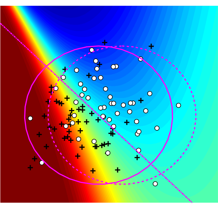
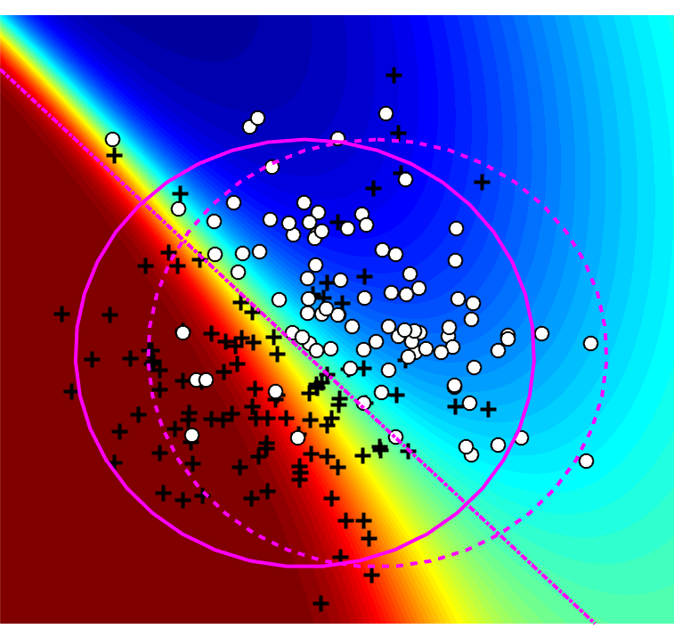
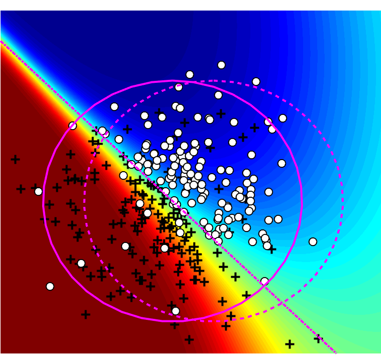
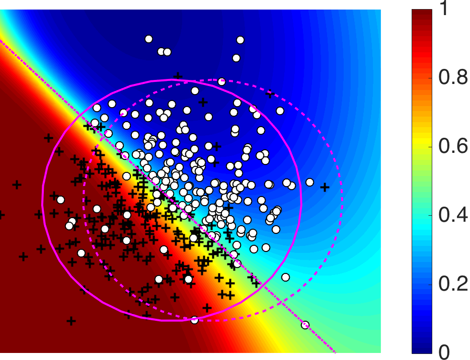
accuracy: 0.760	accuracy: 0.774	accuracy: 0.789	accuracy: 0.815

Figure 3: Convergence of decision boundary in robust bias aware classifier using linear features on 100 samples (a), using Gaussian kernels on 200 samples (b), on 300 samples (c) and on 400 samples (d), with 20% noise in each example. Ellipses show source and target data distribution that closely overlap. The tiled line shows the true decision boundary. With an increasing number of samples and universal kernels, the true decision boundary is recovered with accuracy gradually converging to optimal.

Understanding Kernel RBA

In order to illustrate the effectiveness of kernel RBA, we consider the same datasets from Figure 1 and compare linear RBA and kernel RBA with different kernel types and parameters in Figure 2. Even though kernel methods are usually regarded as a way to introduce non-linearity, its main effect in kernel RBA is the expansion of the constraint space for the adversarial player $\check{P}(Y|X)$ in the two player game in (2). As in Figure 2, kernel RBA achieves better (smaller target logarithmic loss) and more informative (smaller target prediction entropy) predictions in the intersection of source and target distribution, while the true decision boundary is a linear one. Note that here the Gaussian kernel has a large bandwidth to obtain a more linear decision boundary for better visualization. Moreover, the difference between target entropy and logarithmic loss gradually gets smaller in the last three figures. This corresponds with the property of RBA that target logarithmic loss is always upper bounded by the target entropy (with high probability), as proven for a general case in previous literature (?). Therefore, when a larger number of constraints are imposed, i.e., kernel methods are applied, it forms a more restrictive constraint set for $\check{P}(Y|X)$ so that target entropy will bound target loss more and more tightly.

Note that the choice of kernel method and kernel parameters depends on the specific learning problem because we also need to account for overfitting issues in practice. The amount of bias also plays a role in how more source constraints brought by kernel methods help improve over RBA method. Specifically, the larger the bias is, the more RBA will suffer from insufficient constraints from source sample data, which results in larger entropy in target predictions.

Consistency Analysis

We now analyze some theoretical properties of the kernel RBA method. As stated before, kernel RBA directly minimizes the regularized expected target loss. We start with defining this expected target loss explicitly, parameterized by learned $\theta$, at a specific data point $(x,y)$ as: $L_{RBA}(x,y)=\gamma(\theta,x,y)-\log Z$, where $\gamma(\theta,x,y)=\frac{P_{\text{src}}(x)}{P_{\text{trg}}(x)}\theta\Phi(x,y)$ and $\log Z$ is the normalization term.

Theorem 2.

Let $k$ be an bounded universal kernel, and regularization $\lambda$ tending to zero slower than $1/m$ for the kernel RBA method, with $\hat{\theta}$ as the parameter in the resulting predictor, then $\mathbb{E}_{P_{\text{trg}(x,y)}}[L_{RBA}(\hat{\theta},x,y)]-\mathbb{E}_{P_{\text{trg}}(x,y)}[L_{RBA}(\theta^{*},x,y)]\xrightarrow{a.s.}0$.

Proof.

$L_{RBA}$ is a Lipschitz loss because it follows the basic form of logistic loss except $\gamma(\theta,x,y)$ consists of one more component: the density ratio. Given Theorem  1, the minimizer of expected target $L_{RBA}$ can be represented using source samples. It implies that kernel RBA is consistent w.r.t $\mathbb{E}_{P_{\text{trg}(x,y)}}[L_{RBA}(\theta,x,y)]$ when equipped with a universal kernel (?) in source data, assuming $\frac{P_{\text{src}}(x)}{P_{\text{trg}}(x)}$ is accurate, according to consistency properties for Lipschitz loss (?). ∎

Next, we explore whether the optimal expected $L_{RBA}$ on the target distribution $\mathbb{E}_{P_{\text{trg}}(x,y)}[L_{RBA}(\theta^{*},x,y)]$ indicates the optimal 0-1 loss on the target distribution.

Corollary 2 (of Theorem 2).

For any pair of distributions that $P_{\text{src}}(x)>0$, $P_{\text{trg}}(x)>0$ and $P_{\text{src}}(y|x)=P_{\text{trg}}(y|x)$, if $\hat{\eta}(x)$ is the kernel RBA predictor satisfying all the conditions in Theorem  2, then $\mathbb{E}_{P_{\text{trg}}(x,y)}[L_{0-1}(\hat{\eta}(x),y)]-\mathbb{E}_{P_{\text{trg}}(x,y)}[L_{0-1}(\eta^{*}(x),y)]\xrightarrow{a.s.}0$.

Proof.

$L_{RBA}$ is a proper composite loss in both the binary (?) and multi-class cases (?), which means it satisfies $L_{RBA}(\eta,\hat{\eta})-L_{RBA}(\eta,\eta)\geq\frac{C}{2}(\hat{\eta}-\eta)^{2}$ for any $\eta,\hat{\eta}\in[0,1]$, where $\eta$ is the Bayes conditional label probability, $\hat{\eta}$ is the estimated label probability function $\eta(\hat{\theta},x)$ from RBA (4) and $C>0$ is a constant. We then have target expected 0-1 regret be bounded by the expected $L_{RBA}$ regret:

$$\mathbb{E}_{P_{\text{trg}}(x,y)}[L_{0-1}(\hat{h}(x),y)]-\mathbb{E}_{P_{\text{trg}}(x,y)}[L_{0-1}(h^{*}(x),y)]$$

$$\leq 2\sqrt{\mathbb{E}_{P_{\text{trg}}(x,y)}[\hat{\eta}(x)-\eta^{*}(x)]^{2}}$$

$$\leq 2\sqrt{\frac{2}{C}\mathbb{E}_{P_{\text{trg}}(x,y)}[L_{RBA}(\hat{\eta}(x))-L_{RBA}(\eta^{*}(x))]},$$

where $h$ is a predictor function that maps conditional label probability $\eta(x)$ to label. Here the first inequality is due to property of plug-in classifiers and Jensen’s inequality and the second inequality directly comes from the definition of proper loss. Therefore, according to Theorem  2, kernel RBA is consistent w.r.t $L_{RBA}$, and we then conclude that $\mathbb{E}_{P_{\text{trg}}(x,y)}[L_{0-1}(\hat{\eta}(x),y)]-\mathbb{E}_{P_{\text{trg}}(x,y)}[L_{0-1}(\eta^{*}(x),y)]\xrightarrow{a.s.}0$. ∎

Note that employing a universal kernel is a sufficient condition for consistency to hold. Therefore, kernel methods not only provide a larger number of features without increasing computational burdens, but also facilitate the theoretical property to hold for kernel RBA.

We demonstrate how the true decision boundary in the target distribution is recovered with an increasing number of samples when source and target distribution are fairly close in Figure 3. As shown in the first figure, the decision boundary in the linear case is tilted due to the noise. Equipped with more samples and a universal kernel (Gaussian kernel), the decision boundary is shifted to align with the true one. At the same time, the accuracy on target data gets better and better, roughly converging to the optimal. This property of kernel RBA corresponds to Corollary 2 that the 0-1 loss of kernel RBA should converge to the optimal 0-1 loss in the limit.

As a comparison, we show the plots of logloss and accuracy of Kernel IW (solid line) and Kernel Robust (dashed line) methods after 20 repeated experiments using increasing number of samples in Figure 4. The dataset is similar with the example in Figure 3 with 10% noise and source and target distribution closely overlapped. The kernel used here is Gaussian kernel. As shown in the error bars, even though the importance weighted loss converges to the target loss in the limit in theory, it suffers from larger variance and sensitivity to noise in reality when there is only limited number of samples. The reason is that it can be dominated by data with large $P_{\text{trg}}(x)/P_{\text{src}}(x)$ weights, like points with ‘+’ labels in the right-upper corner in Figure 3. Those noise points will push the decision boundary to the left-bottom direction in order to suffer less logloss. On the other hand, Kernel Robust is more robust to noise and keeps reducing the variance and improving the mean logloss and accuracy. This is not only due to the inherently more modest predictions that robust methods produce on biased target distribution, but also due to the consistency property it enjoys as stated in Theorem 2 and Corollary 2. Even though the number of samples is still small and limited here, the source and target distribution is close enough to reflect the convergence tendency with the increasing of source samples.

(a) Logloss	(b) Accuracy

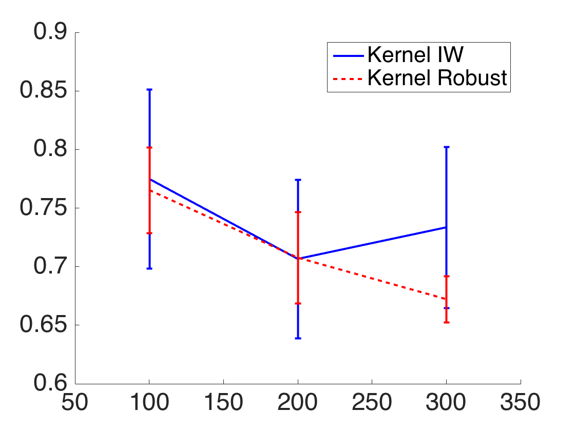
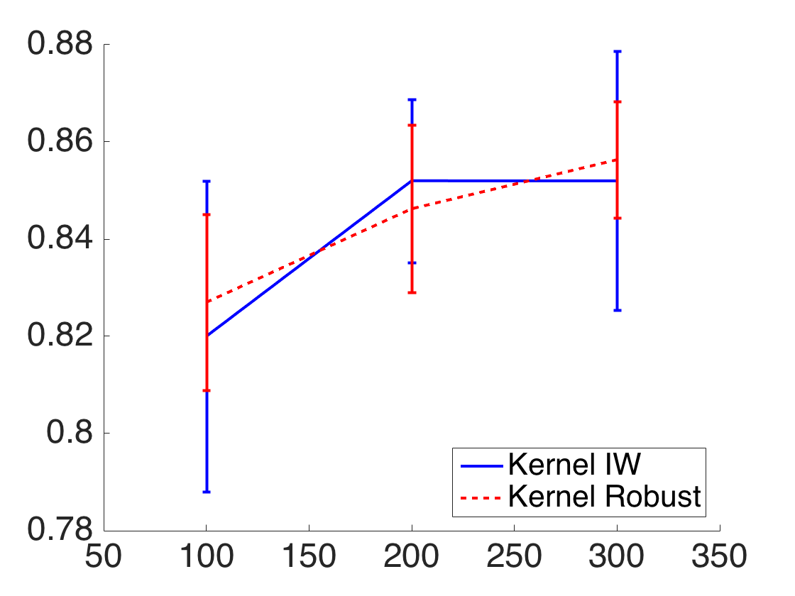
Figure 4: Logloss and accuracy plots as sample size increases from 100 to 300 in kernel IW and kernel Robust methods, with Gaussian kernel, for datasets similar in Figure 3. The error bar shows the 95% confidence interval of the sampling distribution after 20 repeated experiments. IW methods suffer from large variance as robust methods gradually reduce variance and improves on logloss and accuracy more consistently.

Experiments

In this section, we demonstrate the advantages of our kernel RBA approach on datasets that are either synthetically biased via sampling or naturally biased by a differing characteristic or noise. We chose three datasets from the UCI repository (?; ?) for synthetically biased experiments, based on the criteria that each contains approximately 1,000 or more examples and has minimal missing values. They are Vehicle, Segment and Sat. For each dataset, we synthetically generate 20 separate experiments by taking 200 source samples and 200 target data samples from it, generally following the sampling procedure described in ? (?), which we summarize as:

1. Separate the data into source and target portion according to mean of a variable;

2. Randomly sample the target portion as the target dataset;

3. In the source portion, calculate the sample mean $\mu$ and sample covariance $\sigma$, then sample in proportion to weights generated from a multivariate Gaussian with $\mu^{\prime}=\mu/5$ and $\sigma^{\prime}=\sigma/5$ as the source dataset. If the dimension is too large to sample any points, perform PCA first and use the first several principle components to obtain the weights.

We also investigate three naturally biased covariate shift datasets. One of them is Abalone, in which we use the sex variable (male, female, and infant) to create bias. Specifically, we use infant as source samples and the rest as target samples. Note that we use the simplified 3-category classification problem of the Abalone dataset as described in Clark et al. (?) and also sample 200 data points respectively for the source and target datasets. We chose this data because the sex variable makes source-target separation easier and reasonable, and allows the covariate shift assumption to generally hold. In addition, we evaluate our methods on the MNIST dataset (?), which we reduc to binary predictive tasks of differentiating ‘3’ versus ‘8’ and ‘7’ versus ‘9’. We add a biased Gaussian noise with mean 0.2 and standard deviation 0.5 to the testing data to form the covariate shift, i.e. noise $z\sim N(0.2,0.5)$. We randomly sample 2000 training and testing samples and repeat the experiments 20 times. Shown in Figure 5 is the comparison between one batch of training samples and testing samples.

(a) Training Samples	(b) Testing Samples

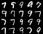
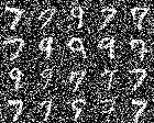
Figure 5: Binarized MNIST data with noise added to the testing set to form covariate shift.

Table 1: Average Target Logloss Comparison

Dataset	Kernel Robust	Kernel LR	Kernel IW	Robust	LR	IW
Vehicle	1.92	16.41	87.69	1.94	8.15	4.94
Segment	2.53	9.62	83.75	2.55	4.37	4.01
Sat	2.44	205.27	111.57	2.57	13.27	8.95
Abalone	1.58	8.52	6.91	1.59	8.73	2.09
MNIST-7v9	0.42	0.44	0.49	0.55	0.80	0.59
MNIST-3v8	0.39	0.46	0.41	0.48	0.84	0.60

Methods

We evaluate our approach and five other methods:
Kernel robust bias aware classifier (Kernel Robust) adversarially minimizes the target distribution logloss using kernel methods, trained using direct gradient calculations as in Corollary 1.
Kernel logistic regression (Kernel LR) ignores the covariate shift and maximizes the source data conditional likelihood, $\max_{\theta}\mathbb{E}_{P_{\text{src}}(x)P{(y|x)}}\left[\log P_{\theta}(Y|X)\right]-\lambda\|\theta\|^{2}_{2}$, where $\hat{P}_{\theta}(y|x)=\frac{\exp(\theta\cdot\Phi(x,y))}{\sum_{y^{\prime}\in\mathcal{Y}}\exp(\theta\cdot\Phi(x,y^{\prime}))}$ and $\lambda$ is the regularization constant.
Kernel importance weighting method (Kernel IW) maximizes the conditional target data likelihood as estimated using importance weighting with the density ratio, $\max_{\theta}\mathbb{E}_{P_{\text{src}}(x)P(y|x)}\left[\frac{P_{\text{trg}}(x)}{P_{\text{src}}(x)}\left(\log P_{\theta}(Y|X)\right)\right]-\lambda\|\theta\|^{2}_{2}$.
Linear robust bias aware prediction (Robust) adversarially minimizes the target distribution logloss without utilizing kernelization , i.e. only first order features are used, trained using direct gradient calculations (6).
Linear logistic regression (LR) utilizes only first order features in the source conditional log likelihood maximization.
Linear importance weighting method (IW) uses first order features only to maximize reweighted source likelihood.

Model Selection

For each kernelized method, we employ a polynomial kernel with order 2. We choose regularization parameter $\lambda$ by 5-fold cross validation, or importance weighted cross validation (IWCV) from $\lambda\in[2^{-16},2^{-12},2^{-8},2^{-4},1]$. We apply traditional cross validation on Kernel LR and LR, and apply IWCV on both importance weighting methods and robust methods. Note that the traditional cross validation process is not correct anymore in the covariate shift setting, because under the covariate shift assumption, the source marginal data distribution of $P(x)$ is different from the target distribution (?). Though IWCV was originally designed for the importance weighting methods, it is proven to be unbiased for any loss function. We apply it to perform model tuning for our robust methods, even though the error estimate variance could be large.

Logistic regression as density estimation

We use a discriminative density estimation method that leverages the logistic regression classifier for estimating the density ratios. According to Bayes rule: $\frac{P_{\text{src}}(x)}{P_{\text{trg}}(x)}=\frac{P(x|\text{``source"})}{P(x|\text{``target"})}=\frac{P(\text{``source"}|x)}{P(\text{``target"}|x)}\frac{P(\text{``target"})}{P(\text{``source"})},$where the second ratio $P(\text{``target"})/P(\text{``source"})$ is computed as the ratio of the number of target and source examples, and the first one is obtained by training a classifier with source data labeled as one class and target data as another class. Similar ideas also appears in recent literature (?). The resulting density ratio of this method is also closely controlled by the amount of regularization. We also choose the regularization weight by cross validation.

Performance Evaluation

We compare average logloss, $\mathbb{E}_{\tilde{P}_{\text{trg}}(x)\tilde{P}(y|x)}[-\log_{2}\hat{P}(Y|X)]$, for each method in Table 1. We perform a paired t-test among each pair of methods. We indicate the methods that have the best performance in bold, along with methods that are statistically indistinguishable from the best (paired t-test with $0.05$ significance level). As shown from the table, the average logloss of the Kernel Robust method is significantly better or not significantly worse than all of the alternatives in all of the datasets. Moreover, we observe the following:

First, logloss of Kernel Robust and Robust is bounded by the uniform distribution baselines, while LR and IW methods can be arbitrary worse when the bias is large, like in Vehicle. This aligns with the properties of robust methods because when the bias is large, the density ratio becomes small and results in uniform predictions. This indicates that robust methods should be preferred if robustness or safety is a concern when the amount of covariate shift is large.

Secondly, Kernel Robust consistently improves the performance from Robust while kernelization may harm LR and IW methods, like in Sat. The reason is when the implicit assumption that (reweighted) source features can be generalize to target distribution in LR and IW does not hold anymore, incorporating larger dimensions of features could make predictions worse. For Kernel Robust and Robust, even though overfitting could still be a concern, the density ratio could adjust the certainty of the prediction and function like a regularizer based on the data’s density in training and testing distribution, so that they suffer less from overfitting.

Finally, we find that Kernel Robust improvement over Robust is related to how far the source input distributions is from the target input distribution. The natural bias in Abalone comes from one feature variable and could be smaller than the bias in synthetic data. This could be why the improvement of logloss in Abalone is smaller than other datasets.

Conclusion

Providing meaningful and robust predictions under covariate shift is challenging. Kernel methods are one avenue for considering large or infinite feature spaces without incurring a proportionate computational burden. We investigated the underlying theoretical foundations for applying kernel methods to RBA by extending the generalized representer theorem, which makes it possible to represent the minimizer of the regularized expected loss with reweighted kernel expectations under the source distribution, and therefore minimize the objective using gradient calculations that only depend on source samples. In addition, we presented the implication of kernel RBA in providing more restrictive feature matching constraints and tighter entropy bounds for target loss, and demonstrated that kernel RBA is both consistent w.r.t its own expected target loss and 0-1 loss. We experimentally validated the advantages of kernelized RBA with synthetically subsampled benchmark data and naturally biased data.

Appendix A SUPPLEMENTARY MATERIALS

Dataset Details

We show the more detailed information about the datasets we used in the experiment in the following tables. We expect the method to also work for higher dimensional dataset when equipped with accurate density ratio estimation. Since the development and analysis of this paper focus more on the Kernel RBA method itself and not on density estimation, we believe smaller datasets are more suitable for the evaluation. We leave the problem of being robust to possibly inaccurate density ratios in higher dimension to future work.

Table 2: Biased Datasets

Dataset	Features	Examples	Classes
Vehicle	18	846	4
Segment	19	2310	7
Sat	36	6435	7
Abalone	7	4177	3
MNIST-3v8	784	5885	2
MNIST-7v9	784	5959	2

Accuracy analysis

We investigate the accuracy (the complement of the misclassification error) of the predictions provided by each of the six approaches on both synthetically biased datasets and naturally biased datasets (in Table 3), where the significant best performance in paired t-test are demonstrated in bold numbers. The significance level here is 0.05. Despite the discrepancy between the logarithmic loss and the misclassification error, the Kernel Robust approach provides statistically better performance than other alternative methods, except on the Abalone dataset. The logarithmic loss is an upper bound of the 0-1 loss. However, the bound can be somewhat loose, so a lower log loss does not necessarily indicate a smaller classification error rate. This is a natural outcome of using logarithmic loss for convenience of optimization. Since logloss is the natural loss measure for probabilistic prediction and is being optimized by all methods (and not accuracy), we validate our method by comparing to other methods using it. Accuracy and logloss do not correlated perfectly, so it is unsurprising that this small difference exists on a measure not being directly optimized.

Table 3: Average Accuracy Comparison

Dataset	Kernel Robust	Kernel LR	Kernel IW	Robust	LR	IW
Vehicle	38%	37%	33%	36%	36%	28%
Segment	71%	70%	37%	67%	68%	36%
Sat	33%	30%	28%	10%	10%	16%
Abalone	46%	43%	42%	48%	47%	39%
MNIST-3v8	88%	86%	86%	87%	75%	85%
MNIST-7v9	87%	85%	86%	86%	71%	83%

References

- [Bache and Lichman 2013] Bache, K., and Lichman, M. 2013. UCI machine learning repository.
- [Ben-David et al. 2007] Ben-David, S.; Blitzer, J.; Crammer, K.; Pereira, F.; et al. 2007. Analysis of representations for domain adaptation. In NIPS.
- [Bickel, Brückner, and Scheffer 2009] Bickel, S.; Brückner, M.; and Scheffer, T. 2009. Discriminative learning under covariate shift. J. Mach. Learn. Res. 10:2137–2155.
- [Clark, Schreter, and Adams 1996] Clark, D.; Schreter, Z.; and Adams, A. 1996. A quantitative comparison of dystal and backpropagation. In Australian Conference on Neural Networks.
- [Cortes et al. 2008] Cortes, C.; Mohri, M.; Riley, M.; and Rostamizadeh, A. 2008. Sample selection bias correction theory. In Algorithmic Learning Theory, 38–53.
- [Cortes, Mansour, and Mohri 2010] Cortes, C.; Mansour, Y.; and Mohri, M. 2010. Learning bounds for importance weighting. In Advances in Neural Information Processing Systems, 442–450.
- [De Vito et al. 2004] De Vito, E.; Rosasco, L.; Caponnetto, A.; Piana, M.; and Verri, A. 2004. Some properties of regularized kernel methods. The Journal of Machine Learning Research 5:1363–1390.
- [Dudík, Schapire, and Phillips 2005] Dudík, M.; Schapire, R. E.; and Phillips, S. J. 2005. Correcting sample selection bias in maximum entropy density estimation. In Advances in Neural Information Processing Systems, 323–330.
- [Fan et al. 2005] Fan, W.; Davidson, I.; Zadrozny, B.; and Yu, P. S. 2005. An improved categorization of classifier’s sensitivity on sample selection bias. In Proc. of the IEEE International Conference on Data Mining, 605–608.
- [Grünwald and Dawid 2004] Grünwald, P. D., and Dawid, A. P. 2004. Game theory, maximum entropy, minimum discrepancy and robust bayesian decision theory. Annals of Statistics 1367–1433.
- [Huang et al. 2006] Huang, J.; Smola, A. J.; Gretton, A.; Borgwardt, K. M.; and Schölkopf, B. 2006. Correcting sample selection bias by unlabeled data. In Neural Information Processing Systems, 601–608.
- [Kanamori, Hido, and Sugiyama 2009] Kanamori, T.; Hido, S.; and Sugiyama, M. 2009. Efficient direct density ratio estimation for non-stationarity adaptation and outlier detection. In Advances in neural information processing systems, 809–816.
- [Kimeldorf and Wahba 1971] Kimeldorf, G., and Wahba, G. 1971. Some results on tchebycheffian spline functions. Journal of Mathematical Analysis and Applications 33(1):82 – 95.
- [LeCun et al. 1998] LeCun, Y.; Bottou, L.; Bengio, Y.; and Haffner, P. 1998. Gradient-based learning applied to document recognition. Proceedings of the IEEE 86(11):2278–2324.
- [Liu and Ziebart 2014] Liu, A., and Ziebart, B. 2014. Robust classification under sample selection bias. In Advances in Neural Information Processing Systems 27, 37–45.
- [Liu, Reyzin, and Ziebart 2015] Liu, A.; Reyzin, L.; and Ziebart, B. D. 2015. Shift-pessimistic active learning using robust bias-aware prediction. In AAAI, 2764–2770.
- [Lopez-Paz and Oquab 2016] Lopez-Paz, D., and Oquab, M. 2016. Revisiting classifier two-sample tests. arXiv preprint arXiv:1610.06545.
- [Micchelli, Xu, and Zhang 2006] Micchelli, C. A.; Xu, Y.; and Zhang, H. 2006. Universal kernels. Journal of Machine Learning Research 7(Dec):2651–2667.
- [Pan and Yang 2010] Pan, S. J., and Yang, Q. 2010. A survey on transfer learning. Knowledge and Data Engineering, IEEE Transactions on 22(10):1345–1359.
- [Reddi and Póczos 2015] Reddi, S. J., and Póczos, B. 2015. Doubly robust covariate shift correction. In AAAI Conference on Artificial Intelligence.
- [Reid and Williamson 2010] Reid, M. D., and Williamson, R. C. 2010. Composite binary losses. Journal of Machine Learning Research 11(Sep):2387–2422.
- [Shimodaira 2000] Shimodaira, H. 2000. Improving predictive inference under covariate shift by weighting the log-likelihood function. Journal of Statistical Planning and Inference 90(2):227–244.
- [Siebert 1987] Siebert, J. P. 1987. Vehicle recognition using rule based methods. Technical report.
- [Steinwart 2005] Steinwart, I. 2005. Consistency of support vector machines and other regularized kernel classifiers. IEEE Transactions on Information Theory 51(1):128–142.
- [Sugiyama and Müller 2005] Sugiyama, M., and Müller, K.-R. 2005. Model selection under covariate shift. In Artificial Neural Networks: Formal Models and Their Applications–ICANN 2005. Springer. 235–240.
- [Sugiyama et al. 2008] Sugiyama, M.; Nakajima, S.; Kashima, H.; Buenau, P. V.; and Kawanabe, M. 2008. Direct importance estimation with model selection and its application to covariate shift adaptation. In Advances in Neural Information Processing Systems, 1433–1440.
- [Sugiyama, Krauledat, and Müller 2007] Sugiyama, M.; Krauledat, M.; and Müller, K.-R. 2007. Covariate shift adaptation by importance weighted cross validation. The Journal of Machine Learning Research 8:985–1005.
- [Vernet, Reid, and Williamson 2011] Vernet, E.; Reid, M. D.; and Williamson, R. C. 2011. Composite multiclass losses. In Advances in Neural Information Processing Systems, 1224–1232.
- [Wen, Yu, and Greiner 2014] Wen, J.; Yu, C.-N.; and Greiner, R. 2014. Robust learning under uncertain test distributions: Relating covariate shift to model misspecification. In International Conference on Machine Learning, 631–639.
- [Yamada et al. 2011] Yamada, M.; Suzuki, T.; Kanamori, T.; Hachiya, H.; and Sugiyama, M. 2011. Relative density-ratio estimation for robust distribution comparison. In Advances in Neural Information Processing Systems, 594–602.
- [Yu and Szepesvári 2012] Yu, Y., and Szepesvári, C. 2012. Analysis of kernel mean matching under covariate shift. In Proc. of the International Conference on Machine Learning, 607–614.
- [Zadrozny 2004] Zadrozny, B. 2004. Learning and evaluating classifiers under sample selection bias. In Proceedings of the International Conference on Machine Learning, 114–121.