Improving the theoretical prediction for the $\bm{B_{s}-\bar{B}_{s}}$ width difference: matrix elements of next-to-leading order $\bm{\Delta B=2}$ operators

Abstract

We present lattice QCD results for the matrix elements of $R_{2}$ and other dimension-7, $\Delta B=2$ operators relevant for calculations of $\Delta\Gamma_{s}$, the $B_{s}-\bar{B}_{s}$ width difference. We have computed correlation functions using 5 ensembles of the MILC Collaboration’s 2+1+1-flavour gauge field configurations, spanning 3 lattice spacings and light sea quarks masses down to the physical point. The HISQ action is used for the valence strange quarks, and the NRQCD action is used for the bottom quarks. Once our analysis is complete, the theoretical uncertainty in the Standard Model prediction for $\Delta\Gamma_{s}$ will be substantially reduced.

1 Introduction

Mixing between particle and antiparticle states of neutral mesons has now been observed in $K^{0}$, $D^{0}$, $B^{0}$, and $B_{s}^{0}$ mesons. These mixings are due to couplings between generations of quark $\mathrm{SU}(2)_{L}$ doublets after electroweak symmetry breaking. Since the leading-order weak process, represented by the “box” diagrams, is at 1-loop level, there is the chance that new heavy particles, beyond those in the Standard Model, could cause differences between Standard Model predictions and experimental results.

To a good approximation, three parameters are sufficient to describe neutral meson mixing: the moduli of the off-diagonal matrix elements of the $2\times 2$ mass and width matrices, $M$ and $\Gamma$, and their relative phase $\phi=\arg(-M_{12}/\Gamma_{12})$. For the $B_{s}^{0}$ system these parameters are constrained by experimental measurements of the $B_{s}^{0}$-$\bar{B}_{s}^{0}$ mass difference, width difference, and a flavour-specific CP asymmetry:

$$\Delta M_{s}=2|M_{12}^{s}|\,,\leavevmode\nobreak\ \leavevmode\nobreak\ \Delta\Gamma_{s}=2|\Gamma_{12}^{s}|\cos\phi_{s}\,,\leavevmode\nobreak\ \mbox{and}\leavevmode\nobreak\ a_{\mathrm{fs}}^{s}=\frac{\Delta\Gamma_{s}}{\Delta M_{s}}\tan\phi_{s}\,.$$ (1)

In (1) and the remainder of this paper we use notation specific to $B_{s}^{0}$ mixing. See Ref. Artuso:2015swg for a recent review of $B_{s}^{0}$ mixing and references to a rich literature.

The calculation of $\Delta\Gamma_{s}$ within the Standard Model is summarized in Ref. Lenz:2006hd . Contributions to $\Gamma_{12}^{s}$ come from matrix elements of the non-local product of 2 $\Delta B=1$ effective Hamiltonians

$$\mathscr{T}=\mathrm{Im}\,i\!\int\!d^{4}x\,\mathcal{T}\,H_{\mathrm{eff}}^{\Delta B=1}(x)\,H_{\mathrm{eff}}^{\Delta B=1}(0)\,.$$ (2)

The contributions from charm and up quarks in the intermediate states depend on the corresponding CKM matrix elements; i.e. $\Gamma_{12}^{s}=-(\lambda_{c}^{2}\Gamma_{12}^{cc}+2\lambda_{c}\lambda_{u}\Gamma_{12}^{uc}+\lambda_{u}^{2}\Gamma_{12}^{uu})$ with $\lambda_{i}=V_{is}^{*}V_{ib}$. At the present level of accuracy, only the CKM-leading contribution from $\Gamma_{12}^{cc}$ is important.

Direct lattice QCD calculation of matrix elements such as $\langle\bar{B}_{s}|\mathscr{T}|B_{s}\rangle$ is not generally feasible due to the difficulty in correctly treating all intermediate states. However, one can employ an operator product expansion known as the heavy quark expansion (HQE). Order-by-order in $\Lambda_{QCD}/m_{B}$, one relates the matrix elements of nonlocal operators to a series of matrix elements of local $\Delta B=2$ operators. Using the most advantageous basis Lenz:2006hd the charm-charm loop contribution to $\Gamma_{12}^{s}$ is given by

$$\Gamma_{12}^{cc}=\frac{G_{F}^{2}m_{b}^{2}}{24\pi m_{B_{s}}}\left[\left(G+\frac{\alpha_{2}}{2}G_{S}\right)\langle\bar{B}_{s}|Q_{1}|{B}_{s}\rangle+\alpha_{1}G_{S}\langle\bar{B}_{s}|Q_{3}|{B}_{s}\rangle\right]\;+\;\tilde{\Gamma}_{12,1/m_{b}}^{cc}\,,$$ (3)

with the next order in the HQE given by

$$\tilde{\Gamma}_{12,1/m_{b}}^{cc}=\frac{G_{F}^{2}m_{b}^{2}}{24\pi m_{B_{s}}}\left\{g_{0}^{cc}\langle\bar{B}_{s}|R_{0}|{B}_{s}\rangle+\sum_{j=1}^{3}\left[g_{j}^{cc}\langle\bar{B}_{s}|R_{j}|{B}_{s}\rangle+\tilde{g}_{j}^{cc}\langle\bar{B}_{s}|\tilde{R}_{j}|{B}_{s}\rangle\right]\right\}\,.$$ (4)

A full basis of dimension-6 $\Delta B=2$ operators can be written as

$$Q_{1} =(\bar{b}^{\alpha}\gamma^{\mu}(1-\gamma^{5})s^{\alpha})(\bar{b}^{\beta}\gamma_{\mu}(1-\gamma^{5})s^{\beta})\,, \leavevmode\nobreak\ \leavevmode\nobreak\ \leavevmode\nobreak\ \leavevmode\nobreak\ Q_{4} =(\bar{b}^{\alpha}(1-\gamma^{5})s^{\alpha})(\bar{b}^{\beta}(1+\gamma^{5})s^{\beta})$$

$$Q_{2} =(\bar{b}^{\alpha}(1-\gamma^{5})s^{\alpha})(\bar{b}^{\beta}(1-\gamma^{5})s^{\beta})\,, \leavevmode\nobreak\ \leavevmode\nobreak\ \leavevmode\nobreak\ \leavevmode\nobreak\ Q_{5} =(\bar{b}^{\alpha}(1-\gamma^{5})s^{\beta})(\bar{b}^{\beta}(1+\gamma^{5})s^{\alpha})$$

$$Q_{3} =(\bar{b}^{\alpha}(1-\gamma^{5})s^{\beta})(\bar{b}^{\beta}(1-\gamma^{5})s^{\alpha})\,.$$ (5)

At higher order in the HQE, one needs matrix elements of the following operators

$$R_{0} =Q_{2}+\alpha_{1}Q_{3}+\frac{1}{2}\alpha_{2}Q_{1}$$

$$R_{1} =\frac{m_{s}}{m_{b}}(\bar{b}^{\alpha}(1-\gamma^{5})s^{\alpha})(\bar{b}^{\beta}(1+\gamma^{5})s^{\beta})=\frac{m_{s}}{m_{b}}Q_{4}$$

$$R_{2} =\frac{1}{m_{b}^{2}}(\bar{b}^{\alpha}\raisebox{0.50003pt}{$\stackrel{{\scriptstyle\scriptstyle\leftarrow}}{{D}}$}_{\rho}\gamma^{\mu}(1-\gamma^{5})D^{\rho}s^{\alpha})(\bar{b}^{\beta}\gamma_{\mu}(1-\gamma^{5})s^{\beta})$$

$$R_{3} =\frac{1}{m_{b}^{2}}(\bar{b}^{\alpha}\raisebox{0.50003pt}{$\stackrel{{\scriptstyle\scriptstyle\leftarrow}}{{D}}$}_{\rho}(1-\gamma^{5})D^{\rho}s^{\alpha})(\bar{b}^{\beta}(1-\gamma^{5})s^{\beta})\,.$$ (6)

Matrix elements of the $Q_{i}$ operators (5) have long been calculated using lattice QCD; unquenched results for $B_{s}$ mixing appear in Gamiz:2009ku ; Carrasco:2013zta ; Dowdall:2014qka ; Bazavov:2016nty . Until this work there have been no calculations of $R_{2}$ and $R_{3}$ matrix elements. In phenomenological analyses Lenz:2006hd ; Jubb:2016mvq the vacuum saturation approximation was used, allowing a 50% uncertainty. Sum rule estimates suggest these matrix elements should be within a few percent of the vacuum saturation approximation values Mannel:2007am , although the VSA predictions depend sensitively on the value of the $b$-quark pole mass.

2 Method

Table 1: Parameters of the ensembles used in this calculation.

label	$a$/fm	$am_{\ell}^{\mathrm{sea}}$	$am_{s}^{\mathrm{sea}}$	$am_{c}^{\mathrm{sea}}$	$N_{s}^{3}\times N_{t}$	$am_{s}^{\mathrm{val}}$	$am_{b}$
VC5	$0.1474(5)(14)(2)$	$0.013$	$0.0650$	$0.838$	$16^{3}\times 48$	$0.0641$	$3.297$
VCp	$0.1450(3)(14)(2)$	$0.00235$	$0.0647$	$0.831$	$32^{3}\times 48$	$0.0628$	$3.25$
C5	$0.1219(2)(9)(2)$	$0.0102$	$0.0509$	$0.635$	$24^{3}\times 64$	$0.0522$	$2.66$
Cp	$0.1189(2)(9)(2)$	$0.00184$	$0.0507$	$0.628$	$48^{3}\times 64$	$0.0507$	$2.62$
F5	$0.0873(2)(5)(1)$	$0.0074$	$0.037$	$0.440$	$32^{3}\times 96$	$0.0364$	$1.91$

We use MILC’s HISQ ensembles, which include sea quark effects of degenerate up and down quarks and physical-mass strange and charm quarks Bazavov:2010ru ; Bazavov:2012xda . We use the HISQ action for the valence $s$ quark and the NRQCD action for the $b$ quark. The 5 ensembles include 3 distinct lattice spacings which we respectively refer to as fine (F), coarse (C), and very coarse (VC). For each of these spacings we use configurations with dynamical pion mass of approximately 300 MeV, and for the coarse and very coarse spacings, we used the physical ensembles which have pion mass approximately 130 MeV. Table 1 lists specific input parameters and the lattice spacings as determined from the $\Upsilon(2S-1S)$ splitting Dowdall:2011wh ; Dowdall:2013tga .

In carrying out the calculation of $\langle\bar{B}_{s}|R_{i}|B_{s}\rangle$, with $i=2,3$, we need not compute all 4 terms in the Lorentz dot product (6). The temporal derivative acting on the $b$ field is $O(m_{b})$: $\bar{b}\raisebox{0.50003pt}{$\stackrel{{\scriptstyle\scriptstyle\leftarrow}}{{D}}$}_{0}=\pm m_{b}\bar{b}\gamma_{0}$, the sign depending on whether we have an outgoing $b$ quark or incoming $\bar{b}$ antiquark. Thus we can write

$$\frac{1}{m_{b}^{2}}(\bar{b}^{\alpha}\raisebox{0.50003pt}{$\stackrel{{\scriptstyle\scriptstyle\leftarrow}}{{D}}$}_{\rho}\Gamma D^{\rho}s^{\alpha})=\frac{1}{m_{b}^{2}}(\bar{b}^{\alpha}\raisebox{0.50003pt}{$\stackrel{{\scriptstyle\scriptstyle\leftarrow}}{{D}}$}_{0}\Gamma D^{0}s^{\alpha})+O\left(\frac{1}{m_{b}^{2}}\right)\,.$$ (7)

Applying the equations of motion, $i\gamma_{0}D^{0}s=(\vec{\gamma}\cdot\vec{D})s$, we arrive at

$$R_{2,3}=\pm\frac{1}{m_{b}}(\bar{b}^{\alpha}\Gamma\gamma_{0}(\vec{\gamma}\cdot\vec{D})s^{\alpha})(\bar{b}^{\beta}\Gamma s^{\beta})\,.$$ (8)

The lattice calculation of $\langle\bar{B}_{s}|R_{2,3}|B_{s}\rangle$ proceeds just as for the $Q_{j}$ matrix elements, except for the need to have a derivative operate on the strange quark at the operator. In addition to needing a staggered propagator $g(y,z)$ computed from local source Wingate:2002fh

$$K(x,y)\,g(y,z)=\delta(x,z)\,,$$ (9)

we need propagators from a point-split source ($k=1,2,3$)

$$K(x,y)\,g^{(k)}(y,z)=\frac{1}{2}\left[\delta(x,z+\hat{k}a)U_{k}^{\dagger}(z)-\delta(x,z-\hat{k}a)U_{k}(z-\hat{k}a)\right]\,.$$ (10)

Naive quark propagators are constructed from staggered propagators via

$$G(y,z) =\Omega(y)\,g(y,z)\,\Omega^{\dagger}(z)$$

$$G^{(k)}(y,z) =\Omega(y)\,g^{(k)}(y,z)\,\Omega^{\dagger}(z\pm\hat{k}a)$$ (11)

where $\Omega(x)=\prod_{\mu=0}^{3}(\gamma_{\mu})^{x_{\mu}/a}$. Since we will need to sum over spatial directions, we require 4 strange quark inversions on each configuration and for each source location.

3 Perturbative matching

One-loop matching between the lattice theory and the continuum $\overline{\mathrm{MS}}$ renormalization schemes has been carried out for the $Q_{i}$ operators, including tree-level $1/m_{b}$ corrections Monahan:2014xra . The 1-loop mixing between operators is parametrized by the $\rho_{ij}$ matrix and $1/m_{b}$ corrections are given by $\hat{Q}_{i,1}^{\mathrm{sub}}$, which are of the form $\frac{1}{2m_{b}}(D_{k}\bar{b}^{\alpha}\gamma^{k}\Gamma_{1}s^{\alpha})(\bar{b}^{\beta}\Gamma_{2}s^{\beta})$:

$$Q_{i}^{\overline{{\scriptscriptstyle\mathrm{MS}}}}=\hat{Q}_{i}+\alpha_{s}\rho_{ij}\hat{Q}_{j}+\hat{Q}_{i,1}^{\mathrm{sub}}\,.$$ (12)

Because derivatives are implemented as finite difference operators the $\frac{1}{a}\hat{Q}_{i}$ mix with $\hat{Q}_{i,1}$; this can similarly be computed in perturbation theory. We define a subtracted operator which gives a more accurate determination of the next-to-leading contribution:

$$\hat{Q}_{i,1}^{\mathrm{sub}}=\hat{Q}_{i,1}-\alpha_{s}\zeta_{ij}\hat{Q}_{j}\,.$$ (13)

The coefficients $\rho_{ij}$ and $\zeta_{ij}$ are tabulated in Monahan:2014xra .

A similar subtraction is done here for the $R_{2,3}$ operators:

$$\hat{R}_{i}^{\mathrm{sub}}=\hat{R}_{i}-\alpha_{s}\xi_{ij}\hat{Q}_{j}\,.$$ (14)

Values for $\xi_{ij}$ are given in Table 2. We use the $\alpha_{V}$ values as tabulated in Colquhoun:2015oha . Note that we have not carried out the 1-loop matching between lattice and $\overline{\mathrm{MS}}$ schemes for $\hat{Q}_{i,1}^{\mathrm{sub}}$ or $\hat{R}_{i}^{\mathrm{sub}}$. Therefore our results for their $\overline{\mathrm{MS}}$ matrix elements will have an $O(\alpha_{s})$ systematic uncertainty.

Table 2: Perturbative subtraction coefficients used in (14), for the values of $am_{b}$ used on each ensemble.

Coefficient	VC5	VCp	C5	Cp	F5
$\xi_{21}$	$-0.1311$	$-0.1327$	$-0.1557$	$-0.1573$	$-0.2004$
$\xi_{22}$	$0.0092$	$0.0093$	$0.013$	$0.0133$	$0.0225$
$\xi_{31}$	$-0.0331$	$-0.0334$	$-0.0392$	$-0.0397$	$-0.0508$
$\xi_{32}$	$-0.2829$	$-0.2864$	$-0.3404$	$-0.3449$	$-0.451$

4 Fits to correlation functions

On each of the 1000 or so configurations in the 5 ensembles listed in Table 1, we created strange quark propagators with inversion sources on 2 timeslices per configuration – except for the VC5 ensemble where we weighed the benefits of doubling the number of sources per configuration. We calculated 3-point functions with local $B_{s}$ and $\bar{B}_{s}$ sinks as well as Gaussian smeared sinks with 2 radii. The smearing was done with the links fixed to Coulomb gauge. The 2-point correlators are taken from earlier work where 16 sources per configuration were used Dowdall:2013tga .

Correlator data are fit to functions of the form

$$C^{\mathrm{2pt}}_{ab}(t) =\sum_{i}X_{a,i}X_{b,i}e^{-E_{i}t}+\sum_{i}(-1)^{t/a}Y_{a,i}Y_{b,i}e^{-E_{i}^{o}t}$$ (15)

and

$$C^{\mathrm{3pt}}_{ab}(t,T) =\sum_{i,j}X_{a,i}V_{nn,ij}X_{b,j}e^{-E_{i}t}e^{-E_{j}(T-t)}\leavevmode\nobreak\ +\leavevmode\nobreak\ \mathrm{oscillating}$$ (17)

using the corrfitter package Lepage:corrfitter . The oscillating states in (LABEL:eq:C2pt) and (17) appear due to opposite-parity temporal doublers present in staggered quark formulations. In (17), $t$ is the temporal distance between the initial state interpolating operator and the 4-quark operator and $T$ is the distance between the initial and final state interpolating operators. Values used in the fits presented here are given in Table 3.

Table 3: Ranges in Euclidean time used for fits to correlation functions. Numbers are given in lattice units.

Ensemble(s)	$t_{\mathrm{min}}$	$t_{\mathrm{max}}^{\mathrm{2pt}}$	$T$
VC5, VCp	5	17	11, 12, 13
C5, Cp	6	21	13, 14, 15, 16
F5	9	40	19, 20, 21, 22, 23, 24, 25

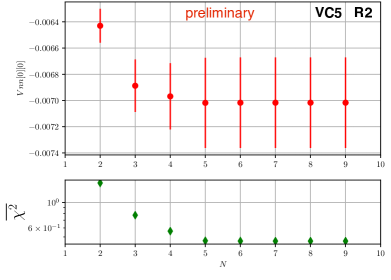
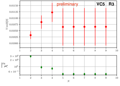
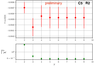
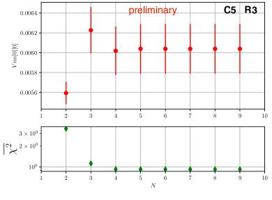
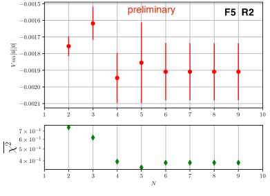
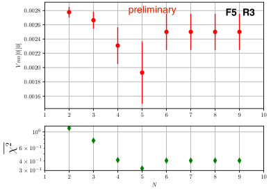
Figure 1: Fit results (upper plots) and $\chi^{2}$ per degree-of-freedom (lower plots) for unsubtracted $R_{2}$ and $R_{3}$ fit amplitudes ($V_{nn,00}$) for increasing number of exponentials (Eq. 17) on the VC5, C5, and F5 ensembles. $N$ is equal to the number of energies in the nonoscillating channel (desired parity) and the number of energies in the oscillating channel.

The Gaussian priors for the fit amplitudes and energies were set as follows. We first performed 2-exponential fits ($N=2$ exponentials in each parity channel) to the 2-point data using wide priors and $t_{\mathrm{min}}\gtrsim 1.2$ fm. From the output of this fit we took the ground state energy and amplitude, multiplied their uncertainties by 10, and used this as the prior means and half-widths for subsequent fits. For the excited states, we took the energy splittings to be $O(a\Lambda_{{\scriptscriptstyle\mathrm{QCD}}})\pm 50\%$ and the amplitudes to be $0\pm 1$.

After fixing the priors for the energies and 2-point amplitudes, we performed $N=3$ fits to 3-point correlator data with $t_{\mathrm{min}}\approx 1.0$ fm and 2 large values of $T$ using $0\pm 1$ for the priors on the $V$ fit parameters. This gave an order-of-magnitude estimate for the ground state amplitude. In subsequent fits we set the prior on $V_{nn,00}$ to be the fit result $\pm 50-100\%$; for the amplitudes in the oscillating terms, we used standard deviations of $100-400\%$ of the results from the preliminary fits.

In the fits presented below, we found that convergence was improved by first fitting the 2-point correlator data and using the results as priors for the fits to the 3-point correlators. In most cases the difference between these “chained” fits and fully simultaneous fits is not significant Bouchard:2014ypa ; however, there were some cases where the simultaneous fits failed to converge.

In Fig. 1 we show preliminary results of fits to the 3-point amplitudes $V_{nn,00}$ determining the $R_{2}$ and $R_{3}$ matrix elements. We observe results which give consistent results once enough exponentials are included to account for excited state contributions to the correlators. In order to obtain this, it was necessary to impose an SVD cut of 0.001 on the correlation matrix whose smaller singular values are not well-determined by the data.

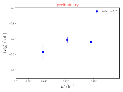
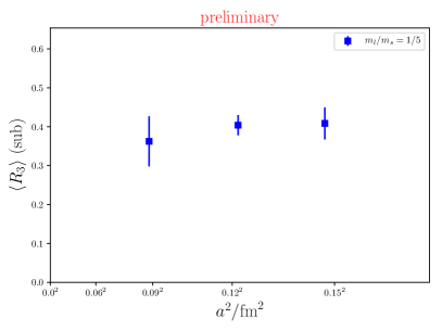
Figure 2 shows preliminary results vs. $a^{2}$ for matrix elements of $R_{2}$ and $R_{3}$ after subtraction (14), on the VC5, C5, and F5 ensembles. The fits on the physical point ensembles VCp and Cp are not as far along in the process of being checked. We are still assessing fitting uncertainties and ensuring results are robust against different fitting choices. What we present here are the results of separate fits to correlators for the operators $R_{2}$, $R_{3}$, $Q_{1}$, and $Q_{2}$. Once we have finished investigating these fits, we will form the linear combinations of correlators, configuration-by-configuration, which will allow us to determine matrix elements of $R_{2}^{\mathrm{sub}}$ and $R_{3}^{\mathrm{sub}}$ directly.

Figure 2: Results (in GeV⁴) for subtracted $R_{2}$ and $R_{3}$ matrix elements on the ensembles with $m_{\ell}/m_{s}=1/5$. Error bars shown only include statistical and fitting uncertainties. The vacuum saturation approximation gives $\langle R_{2}\rangle^{{\scriptscriptstyle\mathrm{VSA}}}=-0.3$ GeV⁴ and $\langle R_{3}\rangle^{{\scriptscriptstyle\mathrm{VSA}}}=0.5$ GeV⁴.

5 Outlook

We presented preliminary results for $\langle\bar{B}_{s}|R_{2}|B_{s}\rangle$ and $\langle\bar{B}_{s}|R_{3}|B_{s}\rangle$ on 5 ensembles spanning a range of 3 lattice spacing and including 2 physical mass ensembles. We are presently verifying stability of fit results. The statistical precision may be improved by performing fits to the linear combinations of correlators directly yielding the 1-loop subtracted matrix elements. The results from different ensembles will then enable an assessment of discretization and quark-mass tuning effects. We expect the dominant uncertainty to be due to the $O(\alpha_{s})$ difference between lattice and continuum regularization schemes. This will be the first time these matrix elements have been computed using lattice QCD.

References

• (1) M. Artuso, G. Borissov, A. Lenz, Rev. Mod. Phys. 88, 045002 (2016), 1511.09466
• (2) A. Lenz, U. Nierste, J. High Energy Phys. 06, 072 (2007), hep-ph/0612167
• (3) Z. Bai, N.H. Christ, T. Izubuchi, C.T. Sachrajda, A. Soni, J. Yu, Phys. Rev. Lett. 113, 112003 (2014), 1406.0916
• (4) E. Gamiz et al. (HPQCD), Phys. Rev. D 80, 014503 (2009), 0902.1815
• (5) N. Carrasco et al. (ETM), JHEP 03, 016 (2014), 1308.1851
• (6) R. Dowdall, C. Davies, R. Horgan, G.P. Lepage, C. Monahan, J. Shigemitsu, PoS LATTICE2014, 373 (2014), 1411.6989
• (7) A. Bazavov et al. (Fermilab Lattice, MILC), Phys. Rev. D 93, 113016 (2016), 1602.03560
• (8) T. Jubb, M. Kirk, A. Lenz, G. Tetlalmatzi-Xolocotzi, Nucl. Phys. B915, 431 (2017), 1603.07770
• (9) T. Mannel, B.D. Pecjak, A.A. Pivovarov (2007), hep-ph/0703244
• (10) A. Bazavov et al. (MILC), Phys. Rev. D 82, 074501 (2010), 1004.0342
• (11) A. Bazavov et al. (MILC), Phys. Rev. D 87, 054505 (2013), 1212.4768
• (12) R. Dowdall et al., Phys. Rev. D 85, 054509 (2012), 1110.6887
• (13) R.J. Dowdall, C.T.H. Davies, R.R. Horgan, C.J. Monahan, J. Shigemitsu, Phys. Rev. Lett. 110, 222003 (2013), 1302.2644
• (14) M. Wingate, J. Shigemitsu, C.T.H. Davies, G.P. Lepage, H.D. Trottier, Phys. Rev. D 67, 054505 (2003), hep-lat/0211014
• (15) C. Monahan, E. Gamiz, R. Horgan, J. Shigemitsu, Phys. Rev. D 90, 054015 (2014), 1407.4040
• (16) B. Colquhoun, C.T.H. Davies, R.J. Dowdall, J. Kettle, J. Koponen, G.P. Lepage, A.T. Lytle, Phys. Rev. D 91, 114509 (2015), 1503.05762
• (17) G.P. Lepage, github.com/gplepage/corrfitter.git
• (18) C.M. Bouchard, G.P. Lepage, C. Monahan, H. Na, J. Shigemitsu, Phys. Rev. D 90, 054506 (2014), 1406.2279
• (19) MILC Code Repository, https://github.com/milc-qcd