Analytical aspects of matrix interpolation problems and its applications

Abstract

In this paper, the $mn$-dimensional space of tensor-product polynomials of two variables, of degree at most $(m-1)+(n-1)$, is considered. A theory of two-variate polynomials is developed by establishing the algebra and basic algebraic properties with respect to the usual addition, scalar multiplication, and a newly defined algebraic operation in the considered space. Further, the existence of the considered space is established with respect to the matrix interpolation problem (MIP), $P(i,j)=a_{ij}$ for all $1\leq i\leq m$, $1\leq j\leq n$, corresponds to a given matrix $(a_{ij})_{m\times n}$ in the space of $m\times n$ order real matrices. The poisedness of the MIP is proved and three formulae are presented to construct the respective polynomial in the considered space. After that, using construction formulae, a polynomial map from the space of $m\times n$ order real matrices to the considered space is defined. Some properties of the polynomial map are investigated and some isomorphic structures between the spaces are installed. It is proved that the considered space is isomorphic to the space of $m\times n$ order real matrices with respect to the algebra structure. The polynomials in the considered space with respect to the MIP’s for the given matrices also preserve the geometric properties of the matrices such as transpose, symmetry, and skew-symmetry. Some examples are included to demonstrate and verify the results.

1 Introduction

Let $\mathbb{R}^{m\times n}$ denotes the space of $m\times n$ order real matrices and $(a_{ij})_{m\times n}$ denotes the matrix $A=(a_{ij})_{m\times n}$, where $m,n\in\mathbb{N}$, [1, 2]. Again, let $\Pi^{d}$ be the space of all $d$-variate polynomials and $\Pi_{N}^{d}$ be ${{d+N}\choose{N}}$-dimensional subspace of $\Pi^{d}$, of degree at most $N$, over the field $\mathbb{F}$, where $d,N\in\mathbb{N}$, [3, 4]. For a given finite linearly independent set $\Theta$ of functionals and an associated vector $Y=(y_{\theta}:\theta\in\Theta)$ of prescribed values, find a polynomial $p$ in $\Pi^{d}$ such that

$$\Theta p=Y,\quad i.e.,\quad\theta p=y_{\theta},\quad\theta\in\Theta,$$ (1)

represents general form of the polynomial interpolation problem, [5, 3].

Let $\mathcal{S}$ be a subspace of $\Pi^{d}$, the polynomial interpolation problem (1) with respect to the set $\Theta$ is said to be poised or correct for $\mathcal{S}$, if for any $Y\in\mathbb{F}^{\Theta}$ there exists a unique $p\in\mathcal{S}$ such that $\Theta p=Y$, [5]. In other words, the interpolation problem (1) with respect to a finite set $\Theta$ of the cardinality $q$, $q\in\mathbb{N}$ is poised in $\mathcal{S}$, if and only if, $q=dim(\mathcal{S})$ and the determinant of the sample matrix, [6, 7],

$$\Theta\mathcal{B}=\begin{bmatrix}\theta p:\theta\in\Theta,p\in\mathcal{B}\end{bmatrix}\in\mathbb{F}^{{\Theta}\times\mathcal{B}}$$ (2)

is non-zero for any choice of basis $\mathcal{B}$ of $\mathcal{S}$. The problem is said to be singular if $det(\Theta\mathcal{B})=0$ for every choice of the set $\Theta$, regular if $det(\Theta\mathcal{B})=0$ for no choice of the set $\Theta$, and almost regular if $det(\Theta\mathcal{B})=0$ only on a subset of $\mathbb{R}^{d}$ of measure zero, [5, 6, 7, 8, 9].

1.1 Motivation and the considered problem

Nowadays, a matrix is the majorly used data structure in computer-oriented models and algorithms of science and engineering. Particularly, in computer graphics [10], signal processing [11], image processing [10, 11], computer-aided designs in control systems [12, 13], thermal engineering [14] to name a few. The generation of the respective three-dimensional smooth interpolating surface is one of the important tools for analysis, comparison, and interpretation. In medical imaging, the surface interpolation plays a very important role in computer-assisted surgical planning and medical diagnosis, [15].

The matrices and matrix algebra are used in a very large-scale to solve the computational problems as their solutions constitute an important and major section of scientific, engineering, and numerical computations on the modern computers. The computational problems build a challenging and application-oriented segment of effectual research. In last decades, an intense research has been witnessed to develop efficient numerical algorithms for the matrix computations and a rapid progress have been noticed in the formation of efficient and effective algorithms for the polynomials in support of algebraic, symbolic, numerical, and scientific computations, [16, 17, 18].

In this regard, considering the matrix interpolation problem [19], defined as follows:

Definition 1.1

Let $(a_{ij})\in\mathbb{R}^{m\times n}$ be a given matrix. For a given subspace $\mathcal{P}$ of $\Pi^{2}$ and the set $\mathcal{D}=\left\{(i,j):i=1,2,\ldots,m,j=1,2,\ldots,n\right\}$ of pairwise distinct interpolation points or nodes, find a polynomial $P\in\mathcal{P}$, such that

$$P(i,j)=a_{ij}\textrm{ for all }i=1,2,\ldots,m,\;j=1,2,\ldots,n$$ (*)

is defined as Matrix Interpolation Problem (MIP).

For the given matrix $(a_{ij})\in\mathbb{R}^{m\times n}$, the MIP (* ‣ 1.1) can not be poised in $\Pi_{N}^{2}$ for almost every $N\in\mathbb{N}$, in view of the fact that,

1. if $mn=dim\Pi_{N}^{2}$, the determinant of the respective sample matrix is zero.

2. if $mn\neq dim\Pi_{N}^{2}$, the necessary condition of $\frac{(N+1)(N+2)}{2}$ interpolation points does not hold (see section 1.1 in [19]).

1.2 Brief review of literature

Let $k$ be a positive integer and $\Theta=\left\{x_{1},x_{2},\ldots,x_{k}\right\}\subset\mathbb{R}^{d}$ be the set of pairwise disjoint points. Then, for a given subspace $\mathcal{H}\subset\Pi^{d}$ and some given constants $f_{1},f_{2},\ldots,f_{k}$ in $\mathbb{R}$, the problem to find a polynomial $p\in\mathcal{H}$ with respect to $\Theta$, such that

$$p(y_{i})=f_{i}\textrm{ for all }i=1,2,...,k$$ (3)

can be defined as Lagrange interpolation problem. The interpolation points $x_{i}$, $i=1,2,...,k$ are called interpolation sites or nodes and $\mathcal{H}$ is known as the interpolation space, [3, 8].

For the given set $\Theta$ and a subspace $\mathcal{H}$, if the problem (3) is poised in $\mathcal{H}$, then the required polynomial $p\in\mathcal{H}$ can be constructed using the interpolation formulae discussed in [4, 6].

In general, the problem (3) need not be poised in a given subspace $\mathcal{H}$ of $\Pi_{N}^{d}$, with respect to the given set $\Theta$ of dimension ${{d+N}\choose{N}}$. As in the case of $d\geq 2$, for a given ${{d+N}\choose{N}}$-dimensional subspace, of a certain total degree, the poisedness of the problem does not independent of the position and geometry (or configuration) of the data points. Also, the basic structure and nature of the interpolation changes utterly and the existence of Haar Spaces of dimension higher than one vanishes, [3, 4, 5, 8].

However, there always exist at least one set $\Theta$ of dimension ${{d+N}\choose{N}}$ in $\mathbb{R}^{d}$ such that the interpolation problem (3) can poised in $\Pi_{N}^{d}$, [4, 5, 8]. Again, the Kergin interpolation [20] insures that, there always exist at least one subspace of $\Pi_{r-1}^{d}$ in which the interpolation problem (3) can be poised for some arbitrarily known set $\Theta$ of dimension $r$, $r\in\mathbb{N}$. Hence, the Lagrange interpolation problem (3) can never be singular, [8]. The work in this manuscript focuses on a special case of two-variate interpolation problem. Therefore, we restrict our self to $d=2$.

For $d=2$, the MIP (* ‣ 1.1) is a class of the Lagrange interpolation problems. Therefore, due to Kergin, there must exist at at least one $mn$-dimensional subspace of $\Pi^{2}$ in which the MIP (* ‣ 1.1) can always be poised with respect to the set $\mathcal{D}$ for a given matrix $a_{ij}\in\mathbb{R}^{m\times n}$. In [19], the constructive existence of two $mn$-dimensional subspaces ${}_{n}^{1}\Pi_{m,n}^{2}$ and ${}_{1}^{m}\Pi_{m,n}^{2}$ has been established, by projecting two-dimensional interpolating points into one-dimension such that all projection are different using a bijective transformation approach and univariate polynomial interpolation, in which the MIP (* ‣ 1.1) can always be poised, where ${}_{\alpha}^{\beta}\Pi_{m,n}^{2}$ is the the space of all two variable polynomials in $x$ and $y$, of degree at most $mn-1$, in two parameters $\alpha$ and $\beta$, with real coefficients, such that, if $P\in{{}_{\alpha}^{\beta}\Pi_{m,n}^{2}}$, then

$$P(x,y)=\sum_{k=0}^{mn-1}{{\lambda_{k}}(\alpha x+\beta y)^{k}}.$$ (4)

Further, it is concluded that the MIP (* ‣ 1.1) can always be poised in ${}_{\alpha}^{\beta}\Pi_{m,n}^{2}$ for unaccountably infinite number of choices of the parameters $\alpha$ and $\beta$, provided the condition $\alpha i_{1}+\beta j_{1}\neq\alpha i_{2}+\beta j_{2}$ for all $i_{1}\neq i_{2}$ and $j_{1}\neq j_{2}$ holds, where $i_{1},i_{2}\in\left\{1,2,\ldots,m\right\}\textrm{ and }j_{1},j_{2}\in\left\{1,2,\ldots,n\right\}$.

From the computational and algebraic point of view, we have identified some flaws of the solutions and the established subspaces which are listed as follows:

1. The degree of the interpolating polynomials is up to $mn-1$, which is somehow high from the computational point of view.

2. The interpolating polynomials in these subspaces, corresponds to the MIP (* ‣ 1.1), do not satisfy the geometric structures of the given matrix $a_{ij}\in\mathbb{R}^{m\times n}$ such as transpose, symmetry, and skew-symmetry.

3. The suggested subspaces are isomorphic to $\mathbb{R}^{m\times n}$ with respect to the vector algebra structure, but they do not preserve multiplication structure as defined in the space of matrices $\mathbb{R}^{m\times n}$.

The identified demerits in the solutions and the interpolation spaces is motivating us to identify at least one $mn$-dimensional space of two variable polynomials, of least possible degree, in which the MIP(* ‣ 1.1) can always be poised and which can preserve almost every algebraic as well as geometric structures of the space $\mathbb{R}^{m\times n}$.

In [21], the author, Seimatsu Narumi suggested a $(m+1)(n+1)$-dimensional space of two variable polynomials, of total degree $mn$ (degree of the variables not greater than $m$ and $n$ respectively). The suggested space is known as the space of tensor-product polynomials in two variable. Narumi claimed this space as a correct interpolation space for a two-variate interpolation problem $P(a_{i},b_{j})=f(a_{i},b_{j})$, corresponds to a two-variate real-valued function $f(x,y)$, by sampling the data with respect to equally spaced interpolation points of the form $(a_{i},b_{j})$, $0\leq i\leq m$, $0\leq j\leq n$. A method of bivariate divided difference is discussed to evaluate the coefficients of the required polynomial in the suggested space, but the existence of the space or the approach of used interpolation method is not mentioned.

For a given matrix $a_{ij}\in\mathbb{R}^{m\times n}$, the MIP (* ‣ 1.1) becomes a special case of the Narumi interpolation problem, where $f:\mathbb{R}^{2}\rightarrow\mathbb{R}$ and the interpolation points takes the form $(i,j)$, $1\leq i\leq m$, $1\leq j\leq n$. Therefore, in this part of work, the $mn$-dimensional space of tensor-product polynomials in two variable, of degree at most $(m-1)+(n-1)$, is considered.

1.3 Objectives and arrangement of the article

The main objective of this paper is to develop a theory of two-variate polynomials in the considered space with respect to the algebraic operations and geometric properties of the space $\mathbb{R}^{m\times n}$. The second objective of this paper is to establish the existence of the considered space in which the MIP(* ‣ 1.1) can be poised for all $a_{ij}\in\mathbb{R}^{m\times n}$ and present some formulae to construct the respective polynomial in the established space. Defining a polynomial map from $\mathbb{R}^{m\times n}$ to the considered space, investigation of some algebraic properties of the polynomial map, and establish some isomorphic structures between the spaces are the other prime objectives.

The rest of the paper is consolidated as follows. In section 2, the $mn$-dimensional space of tensor-product polynomials in two variables, of degree at most $(m-1)+(n-1)$, will be defined. The basic algebra and some algebraic properties of the defined space will be discussed with respect to usual addition, scalar multiplication, and a newly defined algebraic operation. In section 3, the existence of the defined space will be established and the poisedness of the MIP (* ‣ 1.1) in it will be proved. Some formulae will be presented to construct the two-variate polynomial in the space corresponds to the MIP (* ‣ 1.1) for a given matrix $(a_{ij})\in\mathbb{R}^{m\times n}$. In section 4, the polynomial map from $\mathbb{R}^{m\times n}$ to the established subspace will be defined. Some properties of the additive and multiplicative structures will be discussed. In section 5, some examples will be included to validate the theoretical findings and to observe the geometrical prospects. Finally, section 6 will conclude the paper.

2 A theory of two-variate polynomials

In this section, the $mn$-dimensional space of tensor-product polynomial in two variables, of degree at most $(m-1)+(n-1)$, will be defined. Some properties of the defined space will be investigated and a theory of two-variate polynomials will be developed in the defined space with respect to some algebraic operations and geometric properties of the space $\mathbb{R}^{m\times n}$. Some definitions, examples, counterexamples, remarks, and theorems will be included to identify the properties of the defined space.

Definition 2.1

Let $\mathcal{P}_{m}^{n}$ denotes the space of two variable polynomials in $x$ and $y$, of degree at most $(m-1)+(n-1)$, with real coefficients such that, if $P\in\mathcal{P}_{m}^{n}$, then

$$P(x,y)={\sum_{k_{1}=0}^{m-1}{\sum_{k_{2}=0}^{n-1}}}{\lambda_{{k_{1},}{k_{2}}}}{x^{k_{1}}}{y^{k_{2}}}.$$ (**)

Here, dim $\mathcal{P}_{m}^{n}=mn$.

2.1 Equality, addition, and scalar multiplication of the polynomials in $\mathcal{P}_{m}^{n}$

The equality, addition and scalar multiplication of the polynomials in $\mathcal{P}_{m}^{n}$ is defined as the standard definitions of the two-variate polynomials.

Theorem 2.1

The space $\mathcal{P}_{m}^{n}$ is an $mn$-dimensional subspace of $\Pi_{m+n-2}^{2}$.

Proof: The space $\mathcal{P}_{m}^{n}$ is an $mn$-dimensional non-empty subset of the vector space $\Pi_{m+n-2}^{2}$. Suppose $P,Q\in\mathcal{P}_{m}^{n}$ be two polynomials, given as

$$P(x,y)={\sum_{k_{1}=0}^{m-1}{\sum_{k_{2}=0}^{n-1}}}{\lambda_{{k_{1},}{k_{2}}}}{x^{k_{1}}}{y^{k_{2}}},\quad Q(x,y)={\sum_{k_{1}=0}^{m-1}{\sum_{k_{2}=0}^{n-1}}}{\mu_{{k_{1},}{k_{2}}}}{x^{k_{1}}}{y^{k_{2}}},$$

and $\alpha$ be a real scalar. Then,

$$\qquad P(x,y)+Q(x,y) ={\sum_{k_{1}=0}^{m-1}{\sum_{k_{2}=0}^{n-1}}}{\lambda_{{k_{1},}{k_{2}}}}{x^{k_{1}}}{y^{k_{2}}}+{\sum_{k_{1}=0}^{m-1}{\sum_{k_{2}=0}^{n-1}}}{\mu_{{k_{1},}{k_{2}}}}{x^{k_{1}}}{y^{k_{2}}}$$

$$={\sum_{k_{1}=0}^{m-1}{\sum_{k_{2}=0}^{n-1}}}({\lambda_{{k_{1},}{k_{2}}}+\mu_{{k_{1},}{k_{2}}}}){x^{k_{1}}}{y^{k_{2}}},$$

$$\textrm{and }\;\;\alpha P(x,y)=\alpha{\sum_{k_{1}=0}^{m-1}{\sum_{k_{2}=0}^{n-1}}}(\lambda_{{k_{1},}{k_{2}}}){x^{k_{1}}}{y^{k_{2}}}={\sum_{k_{1}=0}^{m-1}{\sum_{k_{2}=0}^{n-1}}}({\alpha}\lambda_{{k_{1},}{k_{2}}}){x^{k_{1}}}{y^{k_{2}}}.$$

i.e., $P(x,y)+Q(x,y),\alpha P(x,y)\in\mathcal{P}_{m}^{n}$ for some scalars $\delta_{{k_{1},}{k_{2}}}={\lambda_{{k_{1},}{k_{2}}}+\mu_{{k_{1},}{k_{2}}}}$ and $\sigma_{{k_{1},}{k_{2}}}={\alpha}\lambda_{{k_{1},}{k_{2}}}$. This completes the proof.

Corollary 2.1

The spaces $\mathbb{R}^{m\times n}$ and $\mathcal{P}_{m}^{n}$ are isomorphic with respect to the vector space structure.

Remark 2.1

The set of standard basis of the vector space $\mathcal{P}_{m}^{n}$, is

$$\left\{x^{k_{1}-1}y^{k_{2}-1}:1\leq k_{1}\leq m,1\leq k_{2}\leq n,\textrm{ where }k_{1},k_{2},m,n\in\mathbb{N}\right\}.$$ (5)

2.2 Product of the polynomials in $\mathcal{P}_{m}^{n}$

Definition 2.2

Let $P\in\mathcal{P}_{m}^{n}$ and $Q\in\mathcal{P}_{n}^{q}$ be two polynomials, then the operation ‘$\otimes$’ given by

$$P(x,y)\otimes Q(x,y)={\sum_{k=1}^{n}(P(x,k)\times Q(k,y))}\textrm{ in }\mathcal{P}_{m}^{q},$$ (6)

is defined as DP product.

Example 2.1

Let $P\in\mathcal{P}_{2}^{2}$ and $Q\in\mathcal{P}_{2}^{3}$ be two polynomials given as $P(x,y)=14x-10xy+13y-18$ and $Q(x,y)=\frac{1}{2}(14y^{2}-11xy^{2}+41xy-34x-52y+44)$ respectively. Then, the definition (2.2) implies that $P(x,y)\otimes Q(x,y)=\frac{1}{2}(60xy^{2}-224xy-79y^{2}+184x+295y-242)$ in $\mathcal{P}_{2}^{3}$. But, $Q(x,y)\otimes P(x,y)$ is not defined.

Remark 2.2

If $P(x,y)\otimes Q(x,y)$ is defined, it is not necessary that $Q(x,y)\otimes P(x,y)$ is also defined.

Example 2.2

Let $P\in\mathcal{P}_{1}^{2}$ and $Q\in\mathcal{P}_{2}^{1}$ be two polynomials given as $P(x,y)=2y-3$ and $Q(x,y)=-2x+3$ respectively. Then, the definition (2.2) implies that $P(x,y)\otimes Q(x,y)=-2\in\mathcal{P}_{1}^{1}$ and $Q(x,y)\otimes P(x,y)=-4xy+6x+6y-9\in\mathcal{P}_{2}^{2}$.

Remark 2.3

If $P\in\mathcal{P}_{m}^{n}$ and $Q\in\mathcal{P}_{p}^{q}$, then $P(x,y)\otimes Q(x,y)$ and $Q(x,y)\otimes P(x,y)$ both are defined, if and only if $n=p$ and $m=q$.

Example 2.3

Let $P\in\mathcal{P}_{2}^{2}$ and $Q\in\mathcal{P}_{2}^{2}$ be two polynomials given as $P(x,y)=-x-y+3$ and $Q(x,y)=-2xy+3i+3j-4$ respectively. Then, the definition (2.2) implies that $P(x,y)\otimes Q(x,y)=y-x\in\mathcal{P}_{2}^{2}$ and $Q(x,y)\otimes P(x,y)=x-y\in\mathcal{P}_{2}^{2}$, Here, $P(x,y)\otimes Q(x,y)\neq Q(x,y)\otimes P(x,y)$.

Remark 2.4

Let $P,Q\in\mathcal{P}_{n}^{n}$, then $P(x,y)\otimes Q(x,y)$ and $Q(x,y)\otimes P(x,y)$ both are defined, but it is not necessary that $P(x,y)\otimes Q(x,y)=Q(x,y)\otimes P(x,y)$.

Example 2.4

Let $P\in\mathcal{P}_{2}^{2}$ and $Q\in\mathcal{P}_{2}^{2}$ be two polynomials given as $P(x,y)=3xy-3x-4y+4$ and $Q(x,y)=2xy-5x-4y+10$ respectively. Then, the definition (2.2) implies that $P(x,y)\otimes Q(x,y)=0\in\mathcal{P}_{2}^{2}$ and $Q(x,y)\otimes P(x,y)=xy-x-2y\in\mathcal{P}_{2}^{2}$.

Remark 2.5

$P(x,y)\otimes Q(x,y)=0$ need not implies that either $P(x,y)=0$ or $Q(x,y)=0$ or $Q(x,y)\otimes P(x,y)=0$, i.e., the set $\mathcal{P}_{n}^{n}$ possess zero-divisor property.

2.2.1 Some properties of the DP product

Theorem 2.2 (DP product closure)

The set $\mathcal{P}_{m}^{n}$ satisfies closure property under the operation $\otimes$, if and only if $m=n$.

Proof: Suppose $\mathcal{P}_{m}^{n}$ satisfies closure property under the operation $`\otimes^{\prime}$, then it has to prove that $m=n$ for all $m,n\in\mathbb{N}$. Let $P_{1},P_{2}\in\mathcal{P}_{m}^{n}$ and if $m\neq n$, then by the definition of DP product (2.2), neither $P_{1}(x,y)\otimes P_{2}(x,y)$ nor $P_{2}(x,y)\otimes P_{1}(x,y)$ is defined. The contra-positive approach of proof, completes the proof of first part.

Conversely, suppose that $m=n$ for all $m,n\in\mathbb{N}$. Let us consider that $P_{1},P_{2}\in\mathcal{P}_{n}^{n}$, then $P_{1}(x,k)\in\mathcal{P}_{n}^{1}$ and $P_{2}(k,y)\in\mathcal{P}_{1}^{n}$, for some fixed $k$, where $1\leq k\leq n$, $n\in\mathbb{N}$. Thus,

$$\quad P_{1}(x,k)\times P_{2}(k,y)\in\mathcal{P}_{n}^{n}\textrm{ for all }1\leq k\leq n\quad\quad\textrm{by definition of DP product}$$

$$\Rightarrow{\sum_{k=1}^{n}(P_{1}(x,k)\times P_{2}(k,y))}\in\mathcal{P}_{n}^{n}\quad\quad\quad\quad\quad\quad\quad\textrm{by additive closure}$$

$$\Rightarrow P_{1}(x,y)\otimes P_{2}(x,y))\in\mathcal{P}_{n}^{n}\quad\quad\quad\quad\quad\quad\quad\quad\quad\textrm{by definition of DP product}$$

This completes the proof.

Theorem 2.3 (DP product and zero polynomial)

Suppose $P\in\mathcal{P}_{m}^{n}$, then

1. $P(x,y)\otimes O(x,y)=0\in\mathcal{P}_{m}^{p}$ for all $O(x,y)=0\in\mathcal{P}_{n}^{p}$,

2. $O(x,y)\otimes P(x,y)=0\in\mathcal{P}_{p}^{n}$ for all $O(x,y)=0\in\mathcal{P}_{p}^{m}$.

Proof: Suppose $P\in\mathcal{P}_{m}^{n}$, then
(i) For all $O(x,y)=0\in\mathcal{P}_{n}^{p}$, we get

$$P(x,y)\otimes O(x,y)={\sum_{k=1}^{n}(P(x,k)\times O(k,y))}={\sum_{k=1}^{n}(P(x,k)\times 0}=0\in\mathcal{P}_{m}^{p}.$$

(ii) For all $O(x,y)=0\in\mathcal{P}_{p}^{m}$, we get

$$O(x,y)\otimes P(x,y)={}{\sum_{k=1}^{n}(O(x,k)\times P(k,y))}={\sum_{k=1}^{n}(0\times P(x,k))}=0\in\mathcal{P}_{p}^{n}.$$

So every entry of the product is the scalar zero, i.e., the result is a zero polynomial. This completes the proof.

Theorem 2.4 (DP product and scalar multiplication)

Suppose $P\in\mathcal{P}_{m}^{n}$, $Q\in\mathcal{P}_{n}^{p}$, and $\alpha$ be a real scalar. Then,

$$\alpha(P(x,y)\otimes Q(x,y))={\left(\alpha P(x,y)\right)}\otimes Q(x,y)=P(x,y)\otimes{\left(\alpha Q(x,y)\right)}\textrm{ in }\mathcal{P}_{m}^{p}.$$

Proof: Let $P\in\mathcal{P}_{m}^{n}$, $Q\in\mathcal{P}_{n}^{p}$ and $\alpha$ be a real scalar. Then,

$$\alpha(P(x,y)\otimes Q(x,y)) =\alpha\left({\sum_{k=1}^{n}{\left(P(x,k)\times Q(k,y)\right)}}\right)\quad\textrm{by definition of DP product}$$

$$=\alpha{\sum_{k=1}^{n}{\left(P(x,k)\times Q(k,y)\right)}}\quad\textrm{by scalar multiplication}$$

$$={\sum_{k=1}^{n}{\alpha\left(P(x,k)\times Q(k,y)\right)}}\quad\textrm{by scalars distribution}$$

$$={\sum_{k=1}^{n}{\left(\left(\alpha P(x,k)\right)\times Q(k,y)\right)}}\quad\textrm{by scalars multiplication}$$

$$={\left(\alpha P(x,y)\right)}\otimes Q(x,y)\quad\textrm{by definition of DP product}$$

so the polynomials $\alpha(P(x,y)\otimes Q(x,y))$ and ${\left(\alpha P(x,y)\right)}\otimes Q(x,y)$ are equal, entry-by-entry, and by the definition of polynomial equality, they are equal polynomials in $\mathcal{P}_{m}^{p}$. Similarly, the polynomials $\alpha(P(x,y)\otimes Q(x,y))$ and $P(x,y)\otimes(\alpha Q(x,y))$ are equal in $\mathcal{P}_{m}^{p}$. This completes the proof.

Theorem 2.5 (DP product associativity)

Suppose $P\in\mathcal{P}_{m}^{n}$, $Q\in\mathcal{P}_{n}^{p}$ and $R\in\mathcal{P}_{p}^{q}$, then

$$P(x,y)\otimes\left(Q(x,y)\otimes R(x,y)\right)=\left(P(x,y)\otimes Q(x,y)\right)\otimes R(x,y)\textrm{ in }\mathcal{P}_{m}^{q}.$$

Proof: Let $P\in\mathcal{P}_{m}^{n}$, $Q\in\mathcal{P}_{n}^{p}$ and $R\in\mathcal{P}_{p}^{q}$. Then, $P(x,y)\otimes\left(Q(x,y)\otimes R(x,y)\right)$

$$=P(x,y)\otimes\left({\sum_{l=1}^{p}{\left(Q(x,l)\times R(l,y)\right)}}\right)\quad\textrm{by definition of DP product}$$

$$={\sum_{k=1}^{n}{\left(P(x,k)\times\left({\sum_{l=1}^{p}{\left(Q(k,l)\times R(l,y)\right)}}\right)\right)}}\quad\textrm{by definition of DP product}$$

$$={\sum_{k=1}^{n}{\sum_{l=1}^{p}}{P(x,k)\times Q(k,l)\times R(l,y)}}\quad\textrm{by distributivity in $\mathbb{R}$}$$

$$={\sum_{l=1}^{p}{\sum_{k=1}^{n}}{P(x,k)\times Q(k,l)\times R(l,y)}}\quad\textrm{by switching the order of finite sums}$$

$$={\sum_{l=1}^{p}{\sum_{k=1}^{n}}{R(l,y)\times P(x,k)\times Q(k,l)}}\quad\textrm{by commutativity in $\mathbb{R}$}$$

$$={\sum_{l=1}^{p}{\left(R(l,y)\times\left({\sum_{k=1}^{n}{\left(P(x,k)\times Q(k,l)\right)}}\right)\right)}}\quad\textrm{since $R(l,y)$ is independent of the index $k$}$$

$$={\sum_{l=1}^{p}{\left(R(l,y)\times\left(P(x,l)\otimes Q(x,l)\right)\right)}}\quad\textrm{by definition of DP product}$$

$$={\sum_{l=1}^{p}{\left(\left(P(x,l)\otimes Q(x,l)\right)\times R(l,y)\right)}}\quad\textrm{by commutativity in $\mathbb{R}$}$$

$$=\left(P(x,y)\otimes Q(x,y)\right)\otimes R(x,y)\quad\textrm{by definition of DP product}$$

So the polynomials $P(x,y)\otimes\left(Q(x,y)\otimes R(x,y)\right)$ and $\left(P(x,y)\otimes Q(x,y)\right)$ $\otimes R(x,y)$ are equal, entry-by-entry, and by the definition of polynomial equality, they are equal polynomial in $\mathcal{P}_{m}^{q}$. This completes the proof.

Theorem 2.6 (DP product distributivity across addition)

Suppose $P,S\in\mathcal{P}_{m}^{n}$ and $Q,R\in\mathcal{P}_{n}^{p}$, then
(i) Left Distributive Law:

$$P(x,y)\otimes{\left(Q(x,y)+R(x,y)\right)}=P(x,y)\otimes Q(x,y)+P(x,y)\otimes R(x,y)\textrm{ in }\mathcal{P}_{m}^{p}.$$

(ii) Right Distributive Law:

$${\left(P(x,y)+S(x,y)\right)}\otimes Q(x,y)=P(x,y)\otimes Q(x,y)+S(x,y)\otimes Q(x,y)\textrm{ in }\mathcal{P}_{m}^{p}.$$

Proof: Let us consider that $P\in\mathcal{P}_{m}^{n}$, $Q\in\mathcal{P}_{n}^{p}$, $R\in\mathcal{P}_{n}^{p}$ and $S\in\mathcal{P}_{m}^{n}$. Then,

$$(i)\textrm{ }P(x,y)\otimes{\left(Q(x,y)+R(x,y)\right)} ={}{\sum_{k=1}^{n}(P(x,k)\times{\left(Q(k,y)+R(k,y)\right)}})$$

$$={}{\sum_{k=1}^{n}{\left(P(x,k)\times Q(k,y)+P(x,k)\times R(k,y)\right)}}$$

$$={}{\sum_{k=1}^{n}{\left(P(x,k)\times Q(k,y)\right)}}+{\sum_{k=1}^{n}{\left(P(x,k)\times R(k,y)\right)}}$$

$$={}P(x,y)\otimes Q(x,y)+P(x,y)\otimes R(x,y).$$

So the polynomials $P(x,y)\otimes{\left(Q(x,y)+R(x,y)\right)}$ and $P(x,y)\otimes Q(x,y)$ + $P(x,y)$ $\otimes R(x,y)$ are equal, entry-by-entry, and by the definition of polynomial equality, they are equal polynomials in $\mathcal{P}_{m}^{p}$.

$$(ii)\textrm{ }{\left(P(x,y)+S(x,y)\right)}\otimes Q(x,y) ={}{\sum_{k=1}^{n}({\left(P(x,k)+S(x,k)\right)\times Q(k,y))}}$$

$$={}{\sum_{k=1}^{n}{\left(P(x,k)\times Q(k,y)+S(x,k)\times Q(k,y)\right)}}$$

$$={}{\sum_{k=1}^{n}{\left(P(x,k)\times Q(k,y)\right)}}+{\sum_{k=1}^{n}{\left(S(x,k)\times Q(k,y)\right)}}$$

$$={}P(x,y)\otimes Q(x,y)+S(x,y)\otimes Q(x,y).$$

So the polynomials ${\left(P(x,y)+S(x,y)\right)}\otimes Q(x,y)$ and $P(x,y)\otimes Q(x,y)$+$S(x,y)$ $\otimes Q(x,y)$ are equal, entry-by-entry, and by the definition of polynomial equality, they are equal polynomials in $\mathcal{P}_{m}^{p}$. This completes the proof.

Definition 2.3 (Identity under DP product)

Let $P\in\mathcal{P}_{m}^{n}$ be any polynomial. Then, the polynomial

1. $I_{n}\in\mathcal{P}_{n}^{n}$ is said to right identity, if $P(x,y)\otimes I_{n}(x,y)=P(x,y)$,

2. $I_{m}\in\mathcal{P}_{m}^{m}$ is said to be left identity, if $I_{m}(x,y)\otimes P(x,y)=P(x,y)$.

In general, the polynomial $I_{n}\in\mathcal{P}_{n}^{n}$ is said to be the identity, if

$$P(x,y)\otimes I_{n}(x,y)=P(x,y)=I_{n}(x,y)\otimes P(x,y)$$ (7)

for all $P\in\mathcal{P}_{n}^{n}$.

Example 2.5

Let $P\in\mathcal{P}_{3}^{2}$, $Q\in\mathcal{P}_{2}^{2}$, and $R\in\mathcal{P}_{3}^{3}$ and be three polynomials given by $P(x,y)=ax^{2}y+bxy+cx^{2}+dx+ey+f$, $Q(x,y)=2xy-3x-3y+5$, and $R(x,y)=\frac{1}{2}(3x^{2}y^{2}-12x^{2}y-12xy^{2}+10x^{2}+49xy+10y^{2}-42x-42y+38)$ respectively. Then, the definition (2.2) implies that $P(x,y)\otimes Q(x,y)=ax^{2}y+bxy+cx^{2}+dx+ey+f$ and $R(x,y)\otimes P(x,y)=ax^{2}y+bxy+cx^{2}+dx+ey+f$. Therefore, $Q\in\mathcal{P}_{2}^{2}$ and $R\in\mathcal{P}_{3}^{3}$ are the right and left identity of $P\in\mathcal{P}_{3}^{2}$ respectively.

Example 2.6

Let $P(x,y)=axy+bx+cy+d$ and $Q(x,y)=2xy-3x-3y+5$ be two polynomials in $\mathcal{P}_{2}^{2}$. Then, the definition (2.2) implies that

$$P(x,y)\otimes Q(x,y)=axy+bx+cy+d=Q(x,y)\otimes P(x,y).$$

Thus, $P(x,y)\otimes Q(x,y)=P(x,y)=Q(x,y)\otimes P(x,y)$ holds. Hence, $Q(x,y)=2xy-3x-3y+5$ is the identity polynomial in $\mathcal{P}_{2}^{2}$.

Remark 2.6

The polynomials $I_{1}(x,y)=1$, $I_{2}(x,y)=2xy-3x-3y+5$, and $I_{3}(x,y)=\frac{1}{2}(3x^{2}y^{2}-12x^{2}y-12xy^{2}+10x^{2}+49xy+10y^{2}-42x-42y+38)$ are the identity polynomials in $\mathcal{P}_{1}^{1}$, $\mathcal{P}_{2}^{2}$ and $\mathcal{P}_{3}^{3}$ respectively.

Definition 2.4 (Inverse under DP product)

Let $P\in\mathcal{P}_{n}^{n}$ be any polynomial. Then, the polynomial $Q\in\mathcal{P}_{n}^{n}$ is said to be the inverse of $P(x,y)$, if

$$P(x,y)\otimes Q(x,y)=I_{n}(x,y)=Q(x,y)\otimes P(x,y),$$ (8)

where $I_{n}\in\mathcal{P}_{n}^{n}$ is the identity polynomial.

Remark 2.7

Let $\alpha_{1},\alpha_{2},\ldots,\alpha_{n}$ be $n$ scalars. The polynomial $P\in\mathcal{P}_{n}^{n}$ is invertible (or non-singular), if

$${\sum_{i=1}^{n}{\alpha_{i}.P(i,y)}}=0\Rightarrow\alpha_{i}=0\textrm{ for all }i=1,2,\ldots,n,$$ (9)

or

$${\sum_{j=1}^{n}{\alpha_{j}.P(x,j)}}=0\Rightarrow\alpha_{j}=0\textrm{ for all }j=1,2,\ldots,m.$$ (10)

Example 2.7

Let $P(x,y)=-10xy+14x+13y-18$ and $Q(x,y)=15xy-21x-20y+28$ be two polynomials in $\mathcal{P}_{2}^{2}$. Suppose $\alpha_{1},\alpha_{2}$ be two scalars, then ${\sum_{i=1}^{2}{\alpha_{i}.P(i,y)}}=0$ and ${\sum_{j=1}^{2}{\alpha_{j}.P(x,j)}}=0$ implies that $\alpha_{1}=\alpha_{2}=0$. Therefore, the polynomial $P\in\mathcal{P}_{2}^{2}$ is invertible. The, the polynomial $Q\in\mathcal{P}_{2}^{2}$ is not invertible, since ${\sum_{i=1}^{2}{\alpha_{i}.P(i,y)}}=0$ implies that $(\alpha_{1},\alpha_{2})=(2k,k)$, where $k$ is an arbitrary constant. Suppose $R\in\mathcal{P}_{2}^{2}$ be the inverse of $P\in\mathcal{P}_{2}^{2}$, given as

$$R(x,y)=\beta_{1}xy+\beta_{2}x+\beta_{3}y+\beta_{4};\quad\beta_{1},\beta_{2},\beta_{3},\beta_{4}\in\mathbb{R}.$$ (11)

Since $I_{2}(x,y)=2xy-3x-3y+5$ is the identity in $\mathcal{P}_{2}^{2}$, therefore the definition (2.4) implies that $\beta_{1}=0$, $\beta_{2}=-\frac{1}{2}$, $\beta_{3}=-1$, and $\beta_{4}=\frac{7}{2}$. Hence, $R(x,y)=-\frac{1}{2}(x+2y-7)$ is the inverse of the given polynomial $P\in\mathcal{P}_{2}^{2}$.

Definition 2.5 (Eigenvalue of the polynomial)

Let $P\in\mathcal{P}_{n}^{n}$ and $X\in\mathcal{P}_{n}^{1}$ be two polynomials. Suppose $\lambda$ is a scalar, if

$$P(x,y)\otimes X(x,1)=\lambda.X(x,1),$$ (12)

then $\lambda$ is said to be “eigenvalue” of the polynomial $P\in\mathcal{P}_{n}^{n}$ and $X\in\mathcal{P}_{n}^{1}$ is the “eigen-polynomial” corresponding to the eigenvalue $\lambda$.

Example 2.8

Let $P\in\mathcal{P}_{2}^{2}$ and $X_{1},X_{2}\in\mathcal{P}_{2}^{1}$ be three polynomials such that $P(x,y)=-xy+4x+3y-5$, $X_{1}(x,1)=5x-8$ and $X_{2}(x,1)=x$. Then,

$$P(x,y)\otimes X_{1}(x,1)=-X_{1}(x,1)\textrm{ and }P(x,y)\otimes X_{2}(x,1)=7X_{2}(x,1).$$

Hence, $\lambda=-1$ and $\lambda=7$ are the eigenvalues of the polynomial $P(x,y)=-xy+4x+3y-5$, where $X_{1}(x,1)=5x-8$ and $X_{2}(x,1)=x$ are the eigen-polynomials corresponding to the eigenvalues $\lambda=-1$ and $\lambda=7$ respectively.

Definition 2.6 (Power of the polynomial)

Let $P\in\mathcal{P}_{n}^{n}$ and $r\geq 2$, $r\in\mathbb{N}$, then

$${\left(P(x,y)\right)}^{2}=P(x,y)\otimes P(x,y)\in\mathcal{P}_{n}^{n}.$$ (13)

Remark 2.8

The polynomial $P\in\mathcal{P}_{n}^{n}$ is said to

1. involuntary, if ${\left(P(x,y)\right)}^{2}=I_{n}(x,y)$, where $I_{n}(x,y)$ is the identity polynomial in $\mathcal{P}_{n}^{n}$.

2. idempotent, if ${\left(P(x,y)\right)}^{2}=P(x,y)$.

3. nilpotent with index $r$, if ${\left(P(x,y)\right)}^{r}=0$, where $r$ is the least positive integer.

4. periodic with index $r$, if ${\left(P(x,y)\right)}^{r+1}=P(x,y)$, where $r$ is the least positive integer.

2.3 Transpose, symmetry, skew-symmetry, and orthogonality of the polynomials in $\mathcal{P}_{m}^{n}$

Definition 2.7 (Transpose of the polynomial)

Let $P(x,y)$ be a polynomial in $\mathcal{P}_{m}^{n}$, then its transpose is defined as

$$P^{T}(x,y)=P(y,x),$$ (14)

such that $P^{T}\in\mathcal{P}_{n}^{m}$.

Remark 2.9

The polynomial $P\in\mathcal{P}_{n}^{n}$ is said to

1. symmetric, if $P(x,y)=P(y,x)$.

2. skew-symmetric, if $P(x,y)=-P(y,x)$.

3. orthogonal, if $P(x,y)\otimes P^{T}(x,y)=I_{n}(x,y)=P^{T}(x,y)\otimes P(x,y)$, where $I_{n}(x,y)$ is the identity polynomial in $\mathcal{P}_{n}^{n}$.

3 Existence of the subspace $\mathcal{P}_{m}^{n}$, poisedness of the MIP, and some polynomial construction formulae

In this section, the existence of the subspace $\mathcal{P}_{m}^{n}$ against the solution of the MIP (* ‣ 1.1) and the poisedness of the MIP (* ‣ 1.1) in it will be proved. Three polynomial construction formulae will be derived using univariate Lagrange, Newton-forward difference, and Newton-backward difference interpolation formulae [22, 23] with respect to the MIP(* ‣ 1.1) for a given matrix $(a_{ij})\in\mathbb{R}^{m\times n}$ in the subspace $\mathcal{P}_{m}^{n}$. Some arguments and other construction methods will be remarked.

Theorem 3.1

Let $a_{ij}\in\mathbb{R}^{m\times n}$ be any given matrix. Then, there exists a unique polynomial $P\in\mathcal{P}_{m}^{n}$ with respect to the set $\mathcal{D}$ which satisfy the MIP (* ‣ 1.1) .

Proof: The proof consist of two parts, existence and uniqueness. Both will be proved one by one as follows:

Existence: Let $A=(a_{ij})\in\mathbb{R}^{m\times n}$ be a given matrix. Then, for the given set of nodes

$$\Omega_{m}=\left\{i:i=1,2,\ldots,n\right\},$$ (15)

associated with the $r$th column, there exists a unique polynomial $p_{r}(x)$ in one variable $x$, of degree at most $m-1$, for all $r=1,2,\ldots,m$, satisfying the problem

$$p_{r}(i)=a_{ir}\textrm{ for all }i=1,2,\ldots,m.$$ (16)

Therefore, the matrix $A=(a_{ij})_{m\times n}$ can be represented as $\begin{pmatrix}p_{1}(x)p_{2}(x)\ldots p_{m}(x)\end{pmatrix}_{1\times n}$. Again, for the given set of nodes

$$\Omega_{n}=\left\{j:j=1,2,\ldots,n\right\},$$ (17)

there exists a unique polynomial $P(x,y)$ in the variable $y$ (for fixed $x$), of degree at most $n-1$, satisfying the problem

$$P(x,j)=p_{j}(x)\textrm{ for all }j=1,2,\ldots,n.$$ (18)

On combing, $P(x,y)$ is a polynomial in $\mathcal{P}_{m}^{n}$, satisfying the MIP (* ‣ 1.1) with respect to the set $\mathcal{D}=\Omega_{m}\times\Omega_{n}$. This completes the proof of existence part.

Uniqueness: The polynomial expressions with respect to the set of nodes (15) can be written as

$$a_{ir}=p_{r}(i)+R_{m,r}(i),\;\;i=1,2,\ldots,m,$$ (19)

where $R_{m,r}(i)$ are the remainders for all $r=1,2,\ldots,n$. The polynomials, satisfy the conditions $a_{kr}=p_{r}(k)$ for all $k=1,2,\ldots,m$. Therefore, the remainder term $R_{m,r}$; $r=1,2,\ldots,n$ vanishes at $i=k$ for all $k=1,2,\ldots,m$. Thus, the polynomials satisfying the conditions (16) are unique for all $r=1,2,\ldots,n$. Again, the polynomial expression with respect to the set of nodes (17) can be written as

$$p_{j}(x)=P(x,j)+R_{n}(j),\;\;j=1,2,\ldots,n,$$ (20)

where $R_{n}(j)$ is the remainder. The polynomial $P(x,j)$, satisfies the conditions $p_{r}(k)=P(x,k)$ for all $k=1,2,\ldots,n$. Therefore, the remainder term $R_{n}$ vanishes at $j=k$ for all $k=1,2,\ldots,n$. Hence, polynomial satisfying the conditions (18) is unique. This completes the theorem.

Remark 3.1

We have used an approach of uni-variate polynomial interpolation for the considered MIP(* ‣ 1.1) and the interpolation space coincide with the space suggested by the author Narumi in the year 1920 in [21]. Narumi had not mentioned the used approach of interpolation for the existence of the space, however a method of bivariate divided difference is used to evaluate the coefficients of the given polynomial form in the suggested space.

Remark 3.2

In general, the interpolation methods assume some certain properties on the sought structure such as smoothness, regularity (nonexistence of some singularities) in a sufficiently large vicinity and so on. The ignorance of these types of assumptions would be dangerous from the error point of view, [24, 25, 26]. We are assuming that the original function is smooth and regular or ‘well-behaved’ in the given domain. The present work is carried out in the algebraic direction and approximation or error estimation is not the part of the article.

In the next theorems, some formulae to construct the unique polynomial $P\in\mathcal{P}_{m}^{n}$ satisfying the MIP (* ‣ 1.1) with respect to the set $\mathcal{D}$ for a given matrix in $\mathbb{R}^{m\times n}$ are formulated using well-known univariate interpolation formulae.

Theorem 3.2

Let $A=(a_{ij})\in\mathbb{R}^{m\times n}$ be a given matrix, then there exist a unique polynomial $P\in\mathcal{P}_{m}^{n}$, satisfying $a_{ij}=P(i,j)$ for all $i=1,2,\ldots,m$, $j=1,2,\ldots,n$, given by

$$P(x,y)=\sum_{r=1}^{n}\left\{\prod_{\alpha=1,\alpha\neq r}^{n}{\frac{(y-\alpha)}{(r-\alpha)}}\right\}{p_{r}(x)},$$ (21)

where

$$\quad p_{r}(x)=\sum_{k=1}^{m}\left\{\prod_{\alpha=1,\alpha\neq k}^{m}{\frac{(x-\alpha)}{(k-\alpha)}}\right\}{a_{kr}}\textrm{ for all }r=1,2,\ldots,n.$$ (22)

Proof: Let $A=(a_{ij})\in\mathbb{R}^{m\times n}$ be a given matrix, then the poisedness of the MIP (* ‣ 1.1) with respect to the set $\mathcal{D}$ of nodes insures that, there exist unique polynomial $P\in\mathcal{P}_{m}^{n}$ satisfying $a_{ij}=P(i,j)$ for all $i=1,2,\ldots,m$,  $j=1,2,\ldots,n$. Using univariate Lagrange interpolation formula, the polynomials with respect to the set of nodes (15), satisfying the problem (16), can be written in the form

$$p_{r}(x)=l_{1,r}(x)a_{1r}+l_{2,r}(x)a_{2r}+\ldots+l_{n,r}(x)a_{nr},$$ (23)

where $l_{k,r}(x)$, $k=1,2,\ldots,m$ are the polynomials of one variable $x$, of degree at most $m-1$ for all $r=1,2,\ldots,n$. The polynomials (23) will satisfy the interpolating conditions (16), if and only if

$$l_{k,r}(x_{i})=\begin{cases}0,&\text{if }k\neq i\\ 1,&\text{if }k=i\end{cases}\textrm{ for all }r=1,2,\ldots,n,$$ (24)

and the polynomials $l_{k,r}(x)$ for all $r=1,2,\ldots,n$, satisfying the conditions (24), can be given as

$$l_{k,r}(x)=\prod_{\alpha=1,\alpha\neq k}^{m}{\frac{(x-\alpha)}{(k-\alpha)}}\textrm{ for all }k=1,2,\ldots,m.$$ (25)

The equations (23) and (25), insured that

$$\quad p_{r}(x)=\sum_{k=1}^{m}\left\{\prod_{\alpha=1,\alpha\neq k}^{m}{\frac{(x-\alpha)}{(k-\alpha)}}\right\}{a_{kr}}\textrm{ for all }r=1,2,\ldots,n.$$

Again, using univariate Lagrange interpolation formula, the polynomial with respect to the set nodes (17), satisfying the problem (18), can be written in the form

$$P(x,y)=L_{1}(y)p_{1}(x)+L_{2}(y)p_{2}(x)+\ldots+L_{n}(y)p_{n}(x),$$ (26)

where $L_{r}(x)$, $r=1,2,\ldots,n$ are the polynomials of one variables $y$, of degree at most $n-1$, i.e., $L_{r}\in\Pi_{n-1}^{1}$. The polynomial (26) will satisfy the interpolating conditions (18), if and only if

$$L_{r}(y_{j})=\begin{cases}0,&\text{if }r\neq j\\ 1,&\text{if }r=j\end{cases},$$ (27)

and the polynomials $L_{r}(y)$, satisfying the conditions (27), can be given as

$$L_{r}(y)=\prod_{\alpha=1,\alpha\neq r}^{n}{\frac{(y-\alpha)}{(r-\alpha)}}\textrm{ for all }r=1,2,\ldots,n.$$ (28)

The combination of the equations (26) and (28), completes the result.

In the similar manner, two more formulae using univariate Newton forward and backward interpolation formulae, for the given set of nodes (15) and (17) satisfying the interpolation problems (16) and (18) respectively, can be given as follows:

Theorem 3.3

Let $A=(a_{ij})\in\mathbb{R}^{m\times n}$ be a given matrix, then there exist a unique polynomial $P\in\mathcal{P}_{m}^{n}$, satisfying $a_{ij}=P(i,j)$ for all $i=1,2,\ldots,m$, $j=1,2,\ldots,n$, given by

$$P(x,y)={} p_{1}(x)+\frac{(y-1)}{1!}{\Delta p_{1}(x)}+\frac{(y-1)(y-2)}{2!}{\Delta^{2}p_{1}(x)}$$ (29)

$$\quad\quad\quad\quad+\ldots+\frac{(y-1)(y-2)\ldots(y-(n-1))}{(n-1)!}{\Delta^{n-1}p_{1}(x)},$$

where

$$\Delta^{r}p_{1}(x)=\sum_{\beta=0}^{r}{(-1)^{\beta}}{r\choose\beta}{p_{r+1-\beta}(x)}\textrm{ for all }r=1,2,\ldots,n-1,$$ (30)

and

$$p_{r}(x)={} a_{1r}+\frac{(x-1)}{1!}{\Delta a_{1r}}+\frac{(x-1)(x-2)}{2!}{\Delta^{2}a_{1r}}$$ (31)

$$\quad\quad\quad\quad\quad\quad+\ldots+\frac{(x-1)(x-2)\ldots(x-(m-1))}{(m-1)!}{\Delta^{m-1}a_{1r}},$$

for all $r=1,2,\ldots,n$, where

$$\Delta^{k}a_{1r}=\sum_{\alpha=0}^{k}{(-1)^{\alpha}}{k\choose\alpha}{a_{(k+1-\alpha)r}}\textrm{ for all }k=1,2,\ldots,m-1.$$ (32)

Theorem 3.4

Let $A=(a_{ij})\in\mathbb{R}^{m\times n}$ be a given matrix, then there exist a unique polynomial $P\in\mathcal{P}_{m}^{n}$, satisfying $a_{ij}=P(i,j)$ for all $i=1,2,\ldots,m$, $j=1,2,\ldots,n$, given by

$$P(x,y)={} p_{n}(x)+\frac{(y-n)}{1!}{\nabla p_{n}(x)}+\frac{(y-n)(y-(n-1))}{2!}{\nabla^{2}p_{n}(x)}$$ (33)

$$\quad\quad\quad\quad+\ldots+\frac{(y-n)(y-(n-1))\ldots(y-2)}{(n-1)!}{\nabla^{n-1}p_{n}(x)},$$

where

$$\nabla^{r}p_{n}(x)=\sum_{\beta=0}^{r}{(-1)^{\beta}}{r\choose\beta}{p_{n-\beta}(x)}\textrm{ for all }r=1,2,\ldots,n-1.$$ (34)

and

$$p_{r}(x)={} a_{mr}+\frac{(x-m)}{1!}{\nabla a_{mr}}+\frac{(x-m)(x-(m-1))}{2!}{\nabla^{2}a_{nr}}$$ (35)

$$\quad\quad\quad\quad\quad\quad+\ldots+\frac{(x-m)(x-(m-1))\ldots(x-2)}{(m-1)!}{\nabla^{m-1}a_{mr}},$$

for all $r=1,2,\ldots,n$, where

$$\nabla^{k}a_{mr}=\sum_{\alpha=0}^{k}{(-1)^{\alpha}}{k\choose\alpha}{a_{(m-\alpha)r}}\textrm{ for all }k=1,2,\ldots,m-1.$$ (36)

Remark 3.3

Suppose $P\in\mathcal{P}_{m}^{n}$ is the unique polynomial of the form (** ‣ 2.1) which satisfy the MIP (* ‣ 1.1) for the given matrix $(a_{ij})\in\mathbb{R}^{m\times n}$. Then, the $mn$ independent conditions $a_{ij}=P(i,j)$ for all $i=1,2,\ldots,m$,  $j=1,2,\ldots,n$ constitute a non-homogeneous linear system of $mn$ equations of the form ${\Lambda}X=\mu$, where $X=(\lambda_{00},\lambda_{01},\ldots,\lambda_{(m-1)(n-1)})^{T}$, $\mu=(a_{11},a_{12},\ldots,a_{mn})^{T}$, and $\Lambda$ is a coefficient matrix. The uniqueness of the solution implies that $det(\Lambda)\neq 0$. Using some suitable method to solve linear system of non-homogeneous equations, the coefficients $\lambda_{k_{1}k_{2}}$, where $k_{1}=0,1,\ldots,m-1$ and $k_{2}=0,1,\ldots,n-1$ can be determined uniquely.

4 Isomorphism and isomorphic structures between the spaces $\mathbb{R}^{m\times n}$ and $\mathcal{P}_{m}^{n}$

Suppose the notation $P_{A}(x,y)$ represent the unique polynomial $P_{A}\in\mathcal{P}_{m}^{n}$ which satisfy the MIP (* ‣ 1.1) for the given matrix $A\in\mathbb{R}^{m\times n}$. This notation will be used frequently in the reaming part of the paper. The spaces $\mathbb{R}^{m\times n}$ and $\mathcal{P}_{m}^{n}$ are isomorphic with respect to the vector spaces structure, therefore there must exist an isomorphism (invertible linear map) between them [2].

Using the result of the theorem 3.1, the polynomial map $D_{p}:\mathbb{R}^{m\times n}\rightarrow\mathcal{P}_{m}^{n}$ can be defined as

$$D_{p}(A)=P_{A}(x,y)\textrm{ for all }A\in\mathbb{R}^{m\times n}.$$ (37)

Again, let the map $f:\mathbb{R}^{m\times n}\times\mathbb{R}^{n\times q}\rightarrow\mathbb{R}^{m\times q}$ is defined as $f(A,B)=A.B$ for all $A\in\mathbb{R}^{m\times n}$, $B\in\mathbb{R}^{n\times q}$, then the composition map $D_{p}of:\mathbb{R}^{m\times n}\times\mathbb{R}^{n\times q}\rightarrow\mathbb{R}^{m\times q}$ is given as $D_{p}of(A,B)=P_{A.B}(x,y)$ for all $A\in\mathbb{R}^{m\times n}$, $B\in\mathbb{R}^{n\times q}$. Also, let the maps $g:\mathbb{R}^{m\times n}\times\mathbb{R}^{n\times q}\rightarrow\mathcal{P}_{m}^{n}\times\mathcal{P}_{n}^{q}$ and $h:\mathcal{P}_{m}^{n}\times\mathcal{P}_{n}^{q}\rightarrow\mathcal{P}_{m}^{q}$ are defined as $g(A,B)=(P_{A}(x,y),P_{B}(x,y))$ for all $A\in\mathbb{R}^{m\times n}$, $B\in\mathbb{R}^{n\times q}$ and $h(P,Q)=P(x,y)\otimes Q(x,y)$ for all $P\in\mathcal{P}_{m}^{n}$, $Q\in\mathcal{P}_{n}^{q}$ respectively. Then, the composition map $hog:\mathbb{R}^{m\times n}\times\mathbb{R}^{n\times q}\rightarrow\mathcal{P}_{m}^{q}$ is given as $hog(A,B)=P_{A}(x,y)\otimes P_{B}(x,y)$ for all $A\in\mathbb{R}^{m\times n}$, $B\in\mathbb{R}^{n\times q}$.

In this section, by proving the invertibility and linearity, it will be proved that the polynomial map (37) is an isomorphism. Further, the property $P_{A.B}(x,y)=P_{A}(x,y)\otimes P_{B}(x,y)$ for all $A\in\mathbb{R}^{m\times n}$, $B\in\mathbb{R}^{n\times q}$ will be proved to establish the discussed product structure. At last, the existence of the identity polynomial under the operation ‘$\otimes$’ will be ensured and it will be proved that the algebraic structures $\langle\mathbb{R}^{n\times n},.\rangle$ and $\langle\mathcal{P}_{n}^{n},\otimes\rangle$ are isomorphic.

Theorem 4.1

For all $P\in\mathcal{P}_{m}^{n}$, there exists a unique matrix $A=(a_{ij})\in\mathbb{R}^{m\times n}$ such that $a_{ij}=P(i,j)$ for all $i=1,2,\ldots,m$, $j=1,2,\ldots,n$.

Theorem 4.2

Let $A,B\in\mathbb{R}^{m\times n}$ and $\alpha$ be a real scalar, then the following properties holds:

1. $P_{A+B}(x,y)=P_{A}(x,y)+P_{B}(x,y)$ in $\mathcal{P}_{m}^{n}$.

2. $P_{\alpha A}(x,y)=\alpha P_{A}(x,y)$ in $\mathcal{P}_{m}^{n}$.

Proof: Let $A,B\in\mathbb{R}^{m\times n}$ be two matrices given as $A=(a_{ij})_{m\times n}$ and $B=(b_{ij})_{m\times n}$. Then, $A+B=(a_{ij}+b_{ij})_{m\times n}$ and $\alpha A=(\alpha a_{ij})_{m\times n}$, for some scalar $\alpha$. Therefore, there exists unique $P_{A}\in\mathcal{P}_{m}^{n}$, $P_{B}\in\mathcal{P}_{m}^{n}$, $P_{A+B}\in\mathcal{P}_{m}^{n}$, and $P_{\alpha A}\in\mathcal{P}_{m}^{n}$, which satisfy the MIP’s

$$P_{A}(i,j)=a_{ij}\textrm{ for all }i=1,2,\ldots,m,\;j=1,2,\ldots,n,$$ (38)

$$P_{B}(i,j)=b_{ij}\textrm{ for all }i=1,2,\ldots,m,\;j=1,2,\ldots,n,$$ (39)

$$P_{A+B}(i,j)=a_{ij}+b_{ij}\textrm{ for all }i=1,2,\ldots,m,\;j=1,2,\ldots,n,$$ (40)

$$\textrm{and }P_{\alpha A}(i,j)=\alpha a_{ij}\textrm{ for all }i=1,2,\ldots,m,\;j=1,2,\ldots,n,$$ (41)

respectively. Again, the definition of usual addition and scalar multiplication of the polynomials in $\mathcal{P}_{m}^{n}$ implies that

$$(i)\;\;P_{A}(i,j)+P_{B}(i,j) =a_{ij}+b_{ij}\textrm{ for all }i=1,2,\ldots,m,\;j=1,2,\ldots,n$$

$$=P_{a+B}(i,j)\textrm{ for all }i=1,2,\ldots,m,\;j=1,2,\ldots,n,$$

$$and\;\;(ii)\;\;\alpha P_{A}(i,j) =\alpha a_{ij}\textrm{ for all }i=1,2,\ldots,m,\;j=1,2,\ldots,n$$

$$=\alpha P_{\alpha A}(i,j)\textrm{ for all }i=1,2,\ldots,m,\;j=1,2,\ldots,n.$$

The MIP (40) and (41) have unique solution in the space $\mathcal{P}_{m}^{n}$ with respect to the set $\mathcal{D}$ by the theorem 3.1. This completes the proof.

Remark 4.1

If $A_{1},A_{2},...,A_{k}\in M_{n,n}$, and $\alpha_{1},\alpha_{2},...,\alpha_{k}$ be some real scalars, then

$$P_{\alpha_{1}{A_{1}}+\alpha_{2}{A_{2}}+...+\alpha_{k}{A_{k}}}(x,y)={\sum_{i=1}^{k}}{\alpha_{i}{P_{A_{i}}(x,y)}}.$$

On combining the theorems 3.1, 4.1, and 4.2, the properties of the polynomial map (37) can be combine as follows.

Theorem 4.3

The polynomial map $D_{p}:\mathbb{R}^{m\times n}\rightarrow\mathcal{P}_{m}^{n}$ defined by

$$D_{p}(A)=P_{A}(x,y)\textrm{ for all }A\in\mathbb{R}^{m\times n}.$$ (42)

is an ispmprphism.

Remark 4.2

The inverse linear map ${D_{p}}^{-1}:\mathcal{P}_{m}^{n}\rightarrow\mathbb{R}^{m\times n}$ is given by

$${D_{p}}^{-1}(P(x,y))={\left[P(i,j)\right]}_{m\times n}\textrm{ for all }P\in\mathcal{P}_{m}^{n}.$$ (43)

Theorem 4.4

Let $A\in\mathbb{R}^{m\times n}$ and $B\in\mathbb{R}^{n\times q}$, then $P_{AB}(x,y)=P_{A}(x,y)\otimes P_{B}(x,y)\textrm{ in }\mathcal{P}_{m}^{q}$.

Proof: Let $A\in\mathbb{R}^{m\times n}$ and $B\in\mathbb{R}^{n\times q}$ be two matrices given as $A=(a_{ij})_{m\times n}$ and $B=(b_{ij})_{n\times p}$. Then,

$$AB=\left({\sum_{k=1}^{n}}{\left(a_{ik}\times b_{kj}\right)}\right)_{m\times q}$$

Therefore, there exists unique $P_{A}\in\mathcal{P}_{m}^{n}$, $P_{B}\in\mathcal{P}_{m}^{n}$ and $P_{AB}\in\mathcal{P}_{m}^{p}$ satisfying the MIP’s

$$P_{A}(i,j)=a_{ij}\textrm{ for all }i=1,2,\ldots,m,\;j=1,2,\ldots,n,$$ (44)

$$P_{B}(i,j)=b_{ij}\textrm{ for all }i=1,2,\ldots,n,\;j=1,2,\ldots,q,$$ (45)

$$P_{AB}(i,j)={\sum_{k=1}^{n}}{\left(a_{ik}\times b_{kj}\right)}\textrm{ for all }i=1,2,\ldots,m,\;j=1,2,\ldots,q,$$ (46)

with respect to the sets $\{(i,j):i=1,2,\ldots,m$,  $j=1,2,\ldots,n\}$, $\{(i,j):i=1,2,\ldots,n$,  $j=1,2,\ldots,q\}$, and $\{(i,j):i=1,2,\ldots,m$,  $j=1,2,\ldots,q\}$ respectively. Again, the definition of DP product (2.2) implies that

$$P_{A}(i,j)\otimes P_{B}(i,j) ={\sum_{k=1}^{n}}{\left(P_{A}(i,k)\times P_{B}(k,j)\right)}\textrm{ for all }i=1,2,\ldots,m,\;j=1,2,\ldots,p$$

$$={\sum_{k=1}^{n}}{\left(a_{ik}\times b_{kj}\right)}\textrm{ for all }i=1,2,\ldots,m,\;j=1,2,\ldots,p$$

$$=P_{AB}(i,j)\textrm{ for all }i=1,2,\ldots,m,\;j=1,2,\ldots,q.$$

Using Theorem 3.1, the MIP (46) with respect to the set $\{(i,j):i=1,2,\ldots,m$,  $j=1,2,\ldots,q\}$ will have unique solution in $\mathcal{P}_{m}^{q}$. This completes the proof.

Remark 4.3

If $A_{1},A_{2},...,A_{k}\in\mathbb{R}^{m\times n}$, $B_{1},B_{2},...,B_{k}\in M_{n,p}$, and $\alpha_{1},\alpha_{2},...,\alpha_{k}$ be some real scalars, then

$$P_{\alpha_{1}{A_{1}}{B_{1}}+\alpha_{2}{A_{2}}{B_{2}}+...+\alpha_{k}{A_{k}}{B_{k}}}(x,y)={\sum_{i=1}^{k}}{\alpha_{i}{\left(P_{A_{i}}(x,y)\otimes P_{B_{i}}(x,y)\right)}}\in\mathcal{P}_{m}^{p}.$$

Corollary 4.1 (Existence of identity polynomial under DP product)

Suppose $P_{A}\in\mathcal{P}_{m}^{n}$, then

1. there exist a $P_{I_{n}}\in\mathcal{P}_{n}^{n}$, such that $P_{A}(x,y)\otimes P_{I_{n}}(x,y)=P_{A}(x,y)$,

2. there exist a $P_{I_{m}}\in\mathcal{P}_{m}^{m}$, such that $P_{I_{m}}(x,y)\otimes P_{A}(x,y)=P_{A}(x,y)$.

The combination of the theorems 4.3 and 4.4 establish a very important result, that can be summarize as follows.

Theorem 4.5

The binary structures $\langle\mathbb{R}^{n\times n},.\rangle$ and $\langle\mathcal{P}_{n}^{n},\otimes\rangle$ are isomorphic.

For $m=n$, the combination of the theorems 2.1, 2.2, 2.5, 2.6 and the corollary 4.1 can be resulted as follows.

Theorem 4.6

The binary structure $\langle\mathcal{P}_{n}^{n},+,\otimes\rangle$ form a ring with unity.

5 Numerical verification

In this section, five examples will be included to illustrate and verify the results.

Example 5.1

Let $\delta\in\mathbb{R}^{1\times 3}$, $\eta\in\mathbb{R}^{3\times 1}$, $\vartheta,\psi\in\mathbb{R}^{2\times 2}$, $\zeta\in\mathbb{R}^{2\times 3}$ and $\theta\in\mathbb{R}^{3\times 2}$ be six matrices $\delta=\begin{pmatrix}1&-1&-2\end{pmatrix}$, $\eta=\begin{pmatrix}-1\\ 1\\ 3\end{pmatrix}$, $\vartheta=\begin{pmatrix}-15&36\\ -1&96\end{pmatrix}$, $\psi=\begin{pmatrix}-216&2\\ 540&-5\end{pmatrix}$, $\zeta=\begin{pmatrix}1&0&2\\ -1&2&-3\end{pmatrix}$ and $\theta=\begin{pmatrix}1&0\\ 0&-1\\ 1&0\end{pmatrix}$ respectively. Therefore, there exists unique $P_{\delta}(1,y)\in\mathcal{P}_{2}^{1}$, $P_{\eta}(x,1)\in\mathcal{P}_{2}^{1}$, $P_{\vartheta}(x,y)\in\mathcal{P}_{2}^{2}$, $P_{\psi}(x,y)\in\mathcal{P}_{2}^{2}$, $P_{\zeta}(x,y)\in\mathcal{P}_{2}^{3}$ and $P_{\theta}(x,y)\in\mathcal{P}_{3}^{2}$ given by $P_{\delta}(1,y)=\frac{1}{2}y^{2}-\frac{7}{2}y+4$, $P_{\eta}(x,1)=2x-3$, $P_{\vartheta}(x,y)=46xy-32x+5y-34$, $P_{\psi}(x,y)=-763xy+1519x+981y-1953$, $P_{\zeta}(x,y)=-\frac{11}{2}xy^{2}+7y^{2}+\frac{41}{2}xy-17x-26y+22$, and $P_{\theta}(x,y)=x^{2}-4x-y+5$ respectively.

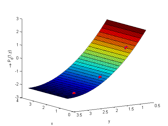
(a) $P_{\delta}\in{\mathcal{P}_{2}^{1}}$

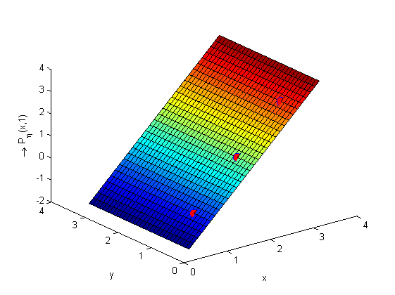
(b) $P_{\eta}\in{\mathcal{P}_{2}^{1}}$

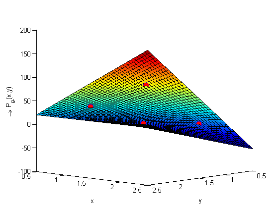
(c) $P_{\vartheta}\in{\mathcal{P}_{2}^{2}}$

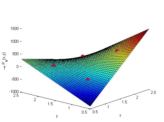
(d) $P_{\psi}\in{\mathcal{P}_{2}^{2}}$

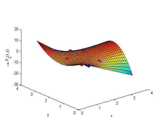
(e) $P_{\zeta}\in{\mathcal{P}_{2}^{3}}$

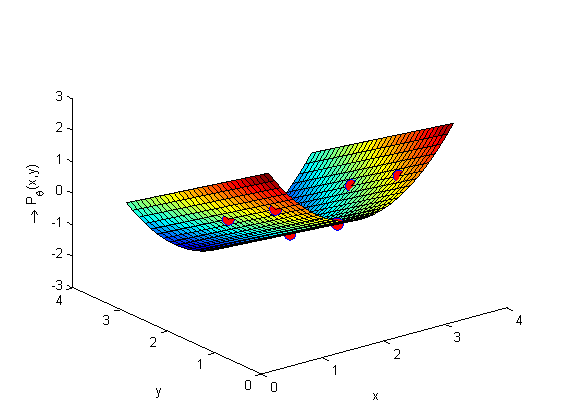
(f) $P_{\theta}\in{\mathcal{P}_{3}^{2}}$

Figure 1: Three-dimensional interpolating surfaces of the polynomials associated to the MIP’s for the given matrices $\delta$, $\eta$, $\vartheta$, $\psi$, $\zeta$ and $\theta$ indicating the data points.

Example 5.2

Let $A_{1}\in\mathbb{R}^{2\times 3}$, $A_{2}\in\mathbb{R}^{3\times 2}$, $A_{3}\in\mathbb{R}^{3\times 3}$, and $A_{4}\in\mathbb{R}^{3\times 3}$ be four matrices given by $A_{1}=\begin{pmatrix}1&-1&2\\ -1&0&-2\end{pmatrix}$, $A_{2}=\begin{pmatrix}1&-1\\ -1&0\\ 2&-2\end{pmatrix}$, $A_{3}=\begin{pmatrix}1&2&3\\ 2&0&4\\ 3&4&-1\end{pmatrix}$, and $A_{4}=\begin{pmatrix}0&1&2\\ -1&0&3\\ -2&-3&0\end{pmatrix}$ respectively. Then, there exists unique $P_{A_{1}}\in\mathcal{P}_{2}^{3}$, $P_{A_{2}}\in\mathcal{P}_{3}^{2}$, $P_{A_{3}}\in\mathcal{P}_{3}^{3}$, and $P_{A_{4}}\in\mathcal{P}_{3}^{3}$ given as

$$P_{A_{1}}(x,y)=-4xy^{2}+\frac{13}{2}y^{2}+15xy-13x-\frac{49}{2}y+21,$$ (47)

$$P_{A_{2}}(x,y)=-4x^{2}y+\frac{13}{2}x^{2}+15xy-\frac{49}{2}x-13y+21,$$ (48)

$$P_{A_{3}}(x,y)=-\frac{9}{2}x^{2}y^{2}+\frac{33}{2}x^{2}y+\frac{33}{2}xy^{2}-\frac{123}{2}xy-12x^{2}-12y^{2}$$ (49)

$$+46x+46y-34,$$

$$\textrm{and }P_{A_{4}}(x,y)=-x^{2}y+xy^{2}+x^{2}-y^{2}-2x+2y,$$ (50)

respectively. Clearly, $P_{A_{1}}(x,y)=P_{A_{2}}^{T}(x,y)$, $P_{A_{3}}(x,y)=P_{A_{3}}^{T}(x,y)$, and $P_{A_{4}}(x,y)=-P_{A_{4}}^{T}(x,y)$. Since $A_{1}=A_{2}^{T}$, $A_{3}=A_{3}^{T}$, and $A_{4}=-A_{4}^{T}$, where $A^{T}$ represents the transpose of the matrix $A$, i.e., the properties of transpose, symmetric and skew-symmetric matrices holds in the associated polynomial subspaces of two variables.

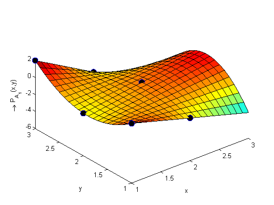
(a) $P_{A_{1}}\in{\mathcal{P}_{2}^{3}}$

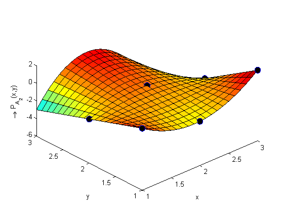
(b) $P_{A_{2}}\in{\mathcal{P}_{3}^{2}}$

(c) $P_{A_{3}}\in{\mathcal{P}_{3}^{3}}$

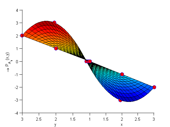
(d) $P_{A_{4}}\in{\mathcal{P}_{3}^{3}}$

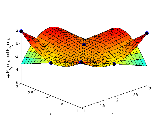
(e) $P_{A_{1}}\in\mathcal{P}_{2}^{3}$ and $P_{A_{2}}\in\mathcal{P}_{3}^{2}$

Figure 2: Three-dimensional interpolating surfaces validating geometric properties of the associated matrices $A_{1}$ $A_{2}$, $A_{3}$ and $A_{4}$ respectively.

Example 5.3

Let $\tau=\begin{pmatrix}-1&2\\ 3&-4\end{pmatrix}$ and $I_{2}=\begin{pmatrix}1&0\\ 0&1\end{pmatrix}$ be the identity matrix in $\mathbb{R}^{2\times 2}$. Then, $\tau^{2}=\begin{pmatrix}7&-10\\ -15&22\end{pmatrix}$ and there exists unique $P_{\tau},P_{\tau^{2}},\textrm{and }P_{I_{2}}\in\mathcal{P}_{2}^{2}$ given as $P_{\tau}(x,y)=-10xy+14x+13y-18$, $P_{\tau^{2}}(x,y)=54xy-76x-71y+100$, and $P_{I_{2}}(x,y)=2xy-3x-3y+5$ respectively. Here, $P_{\tau^{2}}(x,y)+5P_{\tau}(x,y)-2P_{I}(x,y)=0$, i.e.,

$$P_{\tau^{2}}(x,y)-tr(\tau).P_{\tau}(x,y)+det(\tau).P_{I_{2}}(x,y)=0,$$ (51)

i.e., the Cayley-Hamilton theorem holds in the associated polynomial space $\mathcal{P}_{2}^{2}$.

Additionally, since the polynomial $P_{\tau}(x,y)=-10xy+14x+13y-18$, is invertible (see example 2.7). Let $P_{\tau^{-1}}\in\mathcal{P}_{2}^{2}$ be the inverse polynomial. Then, using the equation (51) and definition (2.2), we get

$$P_{\tau^{-1}}(x,y)=\frac{1}{det(\tau)}[-P_{\tau}(x,y)+tr(\tau).P_{I}(x,y)]=-\frac{1}{2}x-y+\frac{7}{2}\in\mathcal{P}_{2}^{2}.$$ (52)

Therefore, $\tau^{-1}=\begin{pmatrix}2&1\\ \frac{3}{2}&\frac{1}{2}\end{pmatrix}$ and it is the required inverse of the matrix $\tau\in\mathbb{R}^{2\times 2}$.

Example 5.4

Let us consider the polynomial map $D_{p}:\mathbb{R}^{2\times 2}\rightarrow\mathcal{P}_{2}^{2}$ defined as

$$D_{p}{\left(\begin{bmatrix}a&b\\ c&d\end{bmatrix}\right)}=(4a-2b -2c+d)+(-2a+2b+c-d)x$$ (53)

$$-(2a-b-2c+d)y+(a-b-c+d)xy.$$

Since, ${D_{p}}{(kA+B)}=k{D_{p}}(A)+{D_{p}}(B)$ for all $A,B\in\mathbb{R}^{2\times 2}$ and non-zero scalar $k$. The map (53) is linear. Again, $B_{1}=\left\{\begin{bmatrix}1&0\\ 0&0\end{bmatrix},\begin{bmatrix}0&1\\ 0&0\end{bmatrix},\begin{bmatrix}0&0\\ 1&0\end{bmatrix},\begin{bmatrix}0&0\\ 0&1\end{bmatrix}\right\}$ and $B_{2}={\{1,x,y,xy\}}$ are the standard bases of the spaces $\mathbb{R}^{2\times 2}$ and $\mathcal{P}_{2}^{2}$ respectively, thus

$$D_{p}{\left(\begin{bmatrix}1&0\\ 0&0\end{bmatrix}\right)}=4-2x-2y+xy,D_{p}{\left(\begin{bmatrix}0&1\\ 0&0\end{bmatrix}\right)}=-2+x+2y-xy,$$

$$D_{p}{\left(\begin{bmatrix}0&0\\ 1&0\end{bmatrix}\right)}=-2+2x+y-xy\textrm{ and }D_{p}{\left(\begin{bmatrix}0&0\\ 0&1\end{bmatrix}\right)}=1-x-y+xy.$$

Therefore, the corresponding co-ordinate matrix with respect to the bases $B_{1}$ and $B_{2}$ is

$$[D_{p}]_{B_{1}}^{B_{2}}=\begin{bmatrix}4&-2&-2&1\\ -2&1&2&-1\\ -2&2&1&-1\\ 1&-1&-1&1\end{bmatrix}_{4\times 4}.$$ (54)

Here, $det\left([D_{p}]_{B_{1}}^{B_{2}}\right)=-1\neq 0$, i.e., $ker(D_{p})=\left\{0\right\}$.

Note 5.1

The inverse linear transformation $D_{p}^{-1}:\mathcal{P}_{2}^{2}\rightarrow\mathbb{R}^{2\times 2}$ is given by

$$D_{p}^{-1}{\left(a+bx+cy+dxy\right)}=\begin{bmatrix}a+b+c+d&a+b+2c+2d\\ a+2b+c+2d&a+2b+2c+4d\end{bmatrix}.$$

The corresponding co-ordinate matrix with respect to the bases $B_{2}$ and $B_{1}$ is

$$[D_{p}^{-1}]_{B_{2}}^{B_{1}}=\begin{bmatrix}1&1&1&1\\ 1&1&2&2\\ 1&2&1&2\\ 1&2&2&4\end{bmatrix}_{4\times 4}.$$ (55)

Clearly,

$$[D_{p}]_{B_{1}}^{B_{2}}.[D_{p}^{-1}]_{B_{2}}^{B_{1}}=\begin{bmatrix}1&0&0&0\\ 0&1&0&0\\ 0&0&1&0\\ 0&0&0&1\end{bmatrix}_{4\times 4}=[D_{p}^{-1}]_{B_{2}}^{B_{1}}.[D_{p}]_{B_{1}}^{B_{2}}.$$

Example 5.5

Let $A_{1}\in\mathbb{R}^{2\times 3}$, $A_{2}\in\mathbb{R}^{3\times 2}$, $A_{3}\in\mathbb{R}^{3\times 3}$, and $A_{4}\in\mathbb{R}^{3\times 3}$ be four matrices given in the example 5.2. Then, ${A_{1}}{A_{2}}=\begin{pmatrix}6&-5\\ -5&5\end{pmatrix}$, ${A_{1}}{A_{3}}=\begin{pmatrix}5&10&-3\\ -7&-10&-1\end{pmatrix}$, ${A_{1}}{A_{4}}=\begin{pmatrix}-3&-5&-1\\ 4&5&-2\end{pmatrix}$, ${A_{2}}{A_{1}}=\begin{pmatrix}2&-1&4\\ -1&1&-2\\ 4&-2&8\end{pmatrix}$, ${A_{3}}{A_{4}}=\begin{pmatrix}-8&-8&8\\ -8&-10&4\\ -2&6&18\end{pmatrix}$, and ${A_{4}}{A_{1}}=\begin{pmatrix}8&8&2\\ 8&10&-6\\ -8&-4&-18\end{pmatrix}$. Therefore, there exists unique $P_{{A_{1}}{A_{2}}}\in\mathcal{P}_{2}^{2}$, $P_{{A_{1}}{A_{3}}}\in\mathcal{P}_{2}^{3}$, $P_{{A_{1}}{A_{4}}}\in\mathcal{P}_{2}^{3}$, $P_{{A_{2}}{A_{1}}}\in\mathcal{P}_{3}^{3}$, $P_{{A_{3}}{A_{4}}}\in\mathcal{P}_{3}^{3}$, and $P_{{A_{4}}{A_{3}}}\in\mathcal{P}_{3}^{3}$ given as

$$P_{{A_{1}}{A_{2}}}(x,y)= {}21xy-32x-32y+49,$$

$$P_{{A_{1}}{A_{3}}}(x,y)= 15xy^{2}-24y^{2}-53xy+26x+85y-44,$$

$$P_{{A_{1}}{A_{4}}}(x,y)= -7xy^{2}+10y^{2}+24xy-10x-35y+15,$$

$$P_{{A_{2}}{A_{1}}}(x,y)= \frac{17}{2}x^{2}y^{2}-32x^{2}y-32xy^{2}+\frac{241}{2}xy+\frac{55}{2}x^{2}+\frac{55}{2}y^{2}-\frac{207}{2}x-\frac{207}{2}y+89,$$

$$P_{{A_{3}}{A_{4}}}(x,y)= -3x^{2}y^{2}+15x^{2}y+9xy^{2}-47xy-9x^{2}+2y^{2}+29x+8y-12,$$

$$\textrm{and }P_{{A_{4}}{A_{3}}}(x,y)= 3x^{2}y^{2}-9x^{2}y-15xy^{2}+47xy-2x^{2}+9y^{2}-8x-29y+12,$$

respectively. The equations (47), (48), (49), and (50) and the definition (2.2) verify that $P_{{A_{1}}{A_{2}}}(x,y)={P_{A_{1}}(x,y)}\otimes{P_{A_{2}}(x,y)}$, $P_{{A_{1}}{A_{3}}}(x,y)={P_{A_{1}}(x,y)}\otimes{P_{A_{3}}(x,y)}$, $P_{{A_{1}}{A_{4}}}(x,y)={P_{A_{1}}(x,y)}\otimes P_{A_{4}}(x,y)$, $P_{{A_{2}}{A_{1}}}(x,y)={P_{A_{2}}(x,y)}\otimes P_{A_{1}}(x,y)$, $P_{{A_{3}}{A_{4}}}(x,y)={P_{A_{3}}(x,y)}\otimes P_{A_{4}}(x,y)$, and $P_{{A_{4}}{A_{3}}}(x,y)={P_{A_{4}}(x,y)}\otimes P_{A_{3}}(x,y)$.

6 Concluding remarks

In this paper, the well known $mn$-dimensional two-variate space of tensor-product polynomials, $\mathcal{P}_{m}^{n}$, of degree at most $(m-1,n-1)$, over the field $\mathbb{R}$ is considered. A theory of two-variable polynomials is developed in $\mathcal{P}_{m}^{n}$, parallel to the basic algebraic operations and geometric properties of the space $\mathbb{R}^{m\times n}$, by establishing the basic algebra and some algebraic properties with respect to the usual addition, scalar multiplication, and a newly defined algebraic operation ‘$\otimes$’. The space $\mathcal{P}_{m}^{n}$ form a subspace of two variable polynomials, of degree at most $m+n-2$ and is isomorphic to $\mathbb{R}^{m\times n}$ with respect to vector algebra structure under usual addition and scalar multiplication operation. Using counterexamples, it is verified that space $\mathcal{P}_{n}^{n}$ is non-commutative and possess zero-divisor property under the operation $\otimes$. It is proved that $\mathcal{P}_{m}^{n}$ is closed under the operation $\otimes$, if $m=n$. Some more algebraic properties of the polynomials in $\mathcal{P}_{m}^{n}$ are discussed under the operation $\otimes$ and it is proved that the associative and distributive law hold. Some definitions are included which define identity, inverse, eigenvalue, and power of the polynomials in $\mathcal{P}_{m}^{n}$ under the operation $\otimes$. In addition, the transpose, symmetry, skew-symmetry, and orthogonality of the polynomials in $\mathcal{P}_{n}^{n}$ is also defined.

In the next section, the existence of the space $\mathcal{P}_{m}^{n}$ is established using tensor-product and univariate polynomial interpolation approach with respect to the MIP(* ‣ 1.1) for a given matrix $(a_{ij})\in\mathbb{R}^{m\times n}$. The poisedness of the MIP(* ‣ 1.1) in $\mathcal{P}_{m}^{n}$ is also ensured. Further, three formulae are derived to construct the polynomial in $\mathcal{P}_{m}^{n}$ which satisfy the MIP(* ‣ 1.1) for a given matrix $(a_{ij})\in\mathbb{R}^{m\times n}$ using well-known univariate interpolation formulae. The method of the non-homogeneous system of linear equations is also remarked to obtain the coefficients of the required polynomial.

The next section focuses on some properties of the established polynomial map from $\mathbb{R}^{m\times n}$ to $\mathcal{P}_{m}^{n}$ on behalf of the construction formulae. It is achieved that the obtained polynomial map is invertible and linear, i.e., is an isomorphism. The respective invertible linear map is also defined. Finally, the multiplicative structure of the polynomials with respect to given matrices is discussed and it is proved that $\langle\mathbb{R}^{n\times n},.\rangle$ and $\langle\mathcal{P}_{n}^{n},\otimes\rangle$ are isomorphic, i.e., the spaces $\mathbb{R}^{n\times n}$ and $\mathcal{P}_{n}^{n}$ are isomorphic with respect to the algebra structure. The existence of the identity polynomial in $\mathcal{P}_{m}^{n}$ under the operation $\otimes$ is also ensured which endorses that $\langle\mathcal{P}_{n}^{n},+,\otimes\rangle$ form a ring with unity over $\mathbb{R}$.

In the last section, five examples are included to validate the results and for geometrical observations. The first example is validating the theorems 3.1, 3.2, 3.3, and 3.4 geometrically by surface diagrams in the figures 1. The second example shows that the polynomials in the associated subspaces preserve the geometric properties of the respective matrices such as transpose, symmetry, and skew-symmetry. In the third example, it is verified that the polynomials in the associated subspace $\mathcal{P}_{2}^{2}$ satisfy the result of Cayley-Hamilton theorem with respect to the given matrix in $\mathbb{R}^{2\times 2}$ and the inverse of the given matrix is also obtained using polynomial algebra. In fourth example, the polynomial map from $\mathbb{R}^{2\times 2}$ to $\mathcal{P}_{2}^{2}$ is defined using the result of the theorems 3.2, 3.3 or 3.4. It is verified that the defined map is linear as well as invertible. The inverse linear map is also included for the cross verification. Finally, last example verify that $P_{{A_{i}}{A_{j}}}(x,y)=P_{A_{i}}(x,y)\otimes P_{A_{j}}(x,y)$ (wherever defined) for $i,j=1,2,3,4$ with respect to the given matrices $A_{1}\in\mathbb{R}^{2\times 3}$, $A_{2}\in\mathbb{R}^{3\times 2}$, $A_{3}\in\mathbb{R}^{3\times 3}$, and $A_{4}\in\mathbb{R}^{3\times 3}$. Theoretical findings and numerical observations assert that space $\mathcal{P}_{m}^{n}$ preserves almost every algebraic and geometrical structure of the space $\mathbb{R}^{m\times n}$.

The transformation of the finite order real matrices $a_{ij}\in\mathbb{R}^{m\times n}$ into $\mathcal{P}_{m}^{n}$, algebraic operations, respective algebra, algebraic and geometric structures, and isomorphism are building some additional tools for algebra, matrix theory, cryptography, and numerical linear algebra community. Considering the rapid growth in the development of the efficient algorithms for the polynomial computation (over matrices), the outcomes can also be beneficial for scientific and numerical computations. In addition, a matrix is a most common data structure to store the complete information of the objects, independent of the content of the data, in the various models of computer graphics, signal processing, image processing, computer-aided designs in control systems, thermal engineering to name a few. Therefore, the generation of the respective three-dimensional smooth interpolating surface (preserving the geometric nature) in the established subspace of two variable polynomials could play some important roles in the stages of analysis, interpretation, and applications.

References

- [1] F. S. Alfio Quarteroni, Riccardo Sacco, Numerical Mathematics. Texts in Applied Mathematics, Springer, Berlin, Heidelberg, 2007.
- [2] S. J. Axler, Linear Algebra Done Right. Undergraduate Texts in Mathematics, Springer International Publishing, third ed., 2015.
- [3] C. De Boor and A. Ron, “Computational aspects of polynomial interpolation in several variables,” Mathematics of Computation, vol. 58, no. 198, pp. 705–727, 1992.
- [4] T. Sauer and Y. Xu, “On multivariate lagrange interpolation,” Mathematics of Computation, vol. 64, no. 211, pp. 1147–1170, 1995.
- [5] T. Sauer, “Polynomial Interpolation in Several Variables: Lattices, Differences, and Ideals,” Studies in Computational Mathematics, vol. 12, pp. 191–230, 2006.
- [6] K. Saniee, “A Simple Expression for Multivariate Lagrange Interpolation,” SIAM Undergraduate Research Online, 2008.
- [7] P. J. Olver, “On Multivariate Interpolation,” Studies in Applied Mathematics, vol. 116, no. 4, pp. 201–240, 2006.
- [8] M. Gasca and T. Sauer, “Polynomial Interpolation in Several Variables,” Advances in Computational Mathematics, vol. 12, pp. 377–410, 2000.
- [9] A. L. M´ehaut´e, “On some aspects of multivariate polynomial interpolation,” Advances in Computational Mathematics, vol. 12, pp. 311–333, 2000.
- [10] S. Levy, L. Velho, A. Frery, and J. Gomes, Image Processing for Computer Graphics and Vision. Texts in Computer Science, Springer London, 2009.
- [11] M. Sonka, V. Hlavac, and R. Boyle, Image Processing, Analysis, and Machine Vision. Cengage Learning, 2014.
- [12] P. Larsen and N. Hansen, Computer Aided Design in Control and Engineering Systems: Advanced Tools for Modern Technology. IFAC proceedings series, Elsevier Science, 2014.
- [13] Z. Chen, Computer Aided Design in Control Systems 1988: Selected Papers from the 4th IFAC Symposium, Beijing, PRC, 23-25 August 1988. IFAC Symposia Series, Elsevier Science, 2017.
- [14] E. Sciubba, G. Manfrida, and U. Desideri, ECOS 2012 The 25th International Conference on Efficiency, Cost, Optimization and Simulation of Energy Conversion Systems and Processes (Perugia, June 26th-June 29th, 2012). Proceedings e report, Firenze University Press, 2012.
- [15] J. C. Carr, W. R. Fright, and R. K. Beatson, “Surface interpolation with radial basis functions for medical imaging,” IEEE transactions on medical imaging, vol. 16, no. 1, pp. 96–107, 1997.
- [16] D. Bini and V. Y. Pan, Polynomial and Matrix Computations (Vol. 1): Fundamental Algorithms. Basel, Switzerland, Switzerland: Birkhauser Verlag, 1994.
- [17] M. G. Anne Bourlioux, Modern Methods in Scientific Computing and Applications. 75, Springer Netherlands, 2002.
- [18] U. Langer and P. Paule, Numerical and Symbolic Scientific Computing: Progress and Prospects. Texts & Monographs in Symbolic Computation, Springer Vienna, 2011.
- [19] S. Dharm Prakash and U. Amit, “Matrix interpolation problem,” https://arxiv.org/abs/1712.08165, 2017.
- [20] P. Kergin, “A natural interpolation of ck functions,” Journal of Approximation Theory, vol. 29, no. 4, pp. 278–293, 1980.
- [21] S. NARUMI, “Some formulas in the theory of interpolation of many independent variables,” Tohoku Mathematical Journal, First Series, vol. 18, pp. 309–321, 1920.
- [22] K. Atkinson, Elementary Numerical Analysis. Wiley, New York, 1985.
- [23] J. R. Jain MK, Iyengar SRK, Numerical methods for scientific and engineering computation. 2nd ed, New Delhi: Wiley Eastern Limited, 1991.
- [24] B. Einarsson, Accuracy and Reliability in Scientific Computing. Software, Environments, and Tools, Society for Industrial and Applied Mathematics (SIAM, 3600 Market Street, Floor 6, Philadelphia, PA 19104), 2005.
- [25] M. Heath, Scientific computing: an introductory survey. McGraw-Hill Higher Education, McGraw-Hill, 2002.
- [26] W. H. Press, S. A. Teukolsky, W. T. Vetterling, and B. P. Flannery, Numerical Recipes 3rd Edition: The Art of Scientific Computing. New York, NY, USA: Cambridge University Press, 3 ed., 2007.