Extrapolating Expected Accuracies for Large Multi-Class Problems

Abstract

The difficulty of multi-class classification generally increases with the number of classes. Using data from a subset of the classes, can we predict how well a classifier will scale with an increased number of classes? Under the assumptions that the classes are sampled identically and independently from a population, and that the classifier is based on independently learned scoring functions, we show that the expected accuracy when the classifier is trained on $k$ classes is the $k-1$st moment of a certain distribution that can be estimated from data. We present an unbiased estimation method based on the theory, and demonstrate its application on a facial recognition example.

1 Introduction

Many machine learning tasks are interested in recognizing or identifying an individual instance within a large set of possible candidates. These problems are usually modeled as multi-class classification problems, with a large and possibly complex label set. Leading examples include detecting the speaker from his voice patterns (Togneri and Pullella, 2011), identifying the author from her written text (Stamatatos et al., 2014), or labeling the object category from its image (Duygulu et al., 2002, Deng et al., 2010, Oquab et al., 2014). In all these examples, the algorithm observes an input $x$, and uses the classifier function $h$ to guess the label $y$ from a large label set $\mathcal{S}$.

There are multiple practical challenges in developing classifiers for large label sets. Collecting high quality training data is perhaps the main obstacle, as the costs scale with the number of classes. It can be affordable to first collect data for a small set of classes, even if the long-term goal is to generalize to a larger set. Furthermore, classifier development can be accelerated by training first on fewer classes, as each training cycle may require substantially less resources. Indeed, due to interest in how small-set performance generalizes to larger sets, such comparisons can found in the literature (Oquab et al., 2014, Griffin et al., 2007). A natural question is: how does changing the size of the label set affect the classification accuracy?

We consider a pair of classification problems on finite label sets: a source task with label set $\mathcal{S}_{k_{1}}$ of size $k_{1}$, and a target task with a larger label set $\mathcal{S}_{k_{2}}$ of size $k_{2}>k_{1}$. For each label set $\mathcal{S}_{k}$, one constructs the classification rule $h^{(k)}:\mathcal{X}\to\mathcal{S}_{k}$. Supposing that in each task, the test example $(X^{*},Y^{*})$ has a joint distribution, define the generalization accuracy for label set $\mathcal{S}_{k}$ as

$$\text{GA}_{k}=\Pr[h^{(k)}(X^{*})=Y^{*}].$$ (1)

The problem of performance extrapolation is the following: using data from only the source task $\mathcal{S}_{k_{1}}$, predict the accuracy for a target task with a larger unobserved label set $\mathcal{S}_{k_{2}}$.

A natural use case for performance extrapolation would be in the deployment of a facial recognition system. Suppose a system was developed in the lab on a database of $k_{1}$ individuals. Clients would like to deploy this system on a new larger set of $k_{2}$ individuals. Performance extrapolation could allow the lab to predict how well the algorithm will perform on the client’s problem, accounting for the difference in label set size.

Extrapolation should be possible when the source and target classifications belong to the same problem domain. In many cases, the set of categories $\mathcal{S}$ is to some degree a random or arbitrary selection out of a larger, perhaps infinite, set of potential categories $\mathcal{Y}$. Yet any specific experiment uses a fixed finite set. For example, categories in the classical Caltech-256 image recognition data set (Griffin et al., 2007) were assembled by aggregating keywords proposed by students and then collecting matching images from the web. The arbitrary nature of the label set is even more apparent in biometric applications (face recognition, authorship, fingerprint identification) where the labels correspond to human individuals (Togneri and Pullella, 2011, Stamatatos et al., 2014). In all these cases, the number of the labels used to define a concrete data set is therefore an experimental choice rather than a property of the domain. Despite the arbitrary nature of these choices, such data sets are viewed as representing the larger problem of recognition within the given domain, in the sense that success on such a data set should inform performance on similar problems.

In this paper, we assume that both $\mathcal{S}_{k_{1}}$ and $\mathcal{S}_{k_{2}}$ are independent identically distributed (i.i.d.) samples from a population (or prior distribution) of labels $\pi$, which is defined on the label space $\mathcal{Y}$. These assumptions help concretely analyze the generalization accuracy, although both are only approximate characterizations of the label selection process, which is often at least partially manual. Since we assume the label set is random, the generalization accuracy of a given classifier becomes a random variable. Performance extrapolation then becomes the problem of estimating the average generalization accuracy $\text{AGA}_{k}$ of an i.i.d. label set $\mathcal{S}_{k}$ of size $k$. The condition of i.i.d. sampling of labels ensures that the separation of labels in a random set $\mathcal{S}_{k_{2}}$ can be inferred by looking at the empirical separation in $\mathcal{S}_{k_{1}}$, and therefore that some estimate of the average accuracy on $\mathcal{S}_{k_{2}}$ can be obtained. We also make the assumption that the classifiers train a separate model for each class. This convenient property allows us to characterize the accuracy of the classifier by selectively conditioning on one class at a time.

Our paper presents two main contributions related to extrapolation. First, we present a theoretical formula describing how average accuracy for smaller $k$ is linked to average accuracy for label set of size $K>k$. We show that accuracy at any size depends on a discriminability function ${D}$, which is determined by properties of the data distribution and the classifier. Second, we propose an estimation procedure that allows extrapolation of the observed average accuracy curve from $k_{1}$-class data to a larger number of classes, based on the theoretical formula. Under certain conditions, the estimation method has the property of being an unbiased estimator of the average accuracy.

The paper is organized as follows. In the rest of this section, we discuss related work. The framework of randomized classification is introduced in Section 2, and there we also introduce a toy example which is revisited throughout the paper. Section 3 develops our theory of extrapolation, and Section 3.3 we suggest an estimation method. We evaluate our method using simulations in Section 4. In Section 5, we demonstrate our method on a facial recognition problem, as well as an optical character recognition problem. In Section 6 we discuss modeling choices and limitations of our theory, as well as potential extensions.

1.1 Related Work

Linking performance between two different but related classification tasks can be considered an instance of transfer learning (Pan and Yang, 2010). Under Pan and Yang’s terminology, our setup is an example of multi-task learning, because the source task has labeled data, which is used to predict performance on a target task that also has labeled data. Applied examples of transfer learning from one label set to another include Oquab et al. (2014), Donahue et al. (2014), Sharif Razavian et al. (2014). However, there is little theory for predicting the behavior of the learned classifier on a new label set. Instead, most research classification for large label sets deal with the computational challenges of jointly optimizing the many parameters required for these models for specific classification algorithms (Crammer and Singer, 2001, Lee et al., 2004, Weston and Watkins, 1999). Gupta et al. (2014) presents a method for estimating the accuracy of a classifier which can be used to improve performance for general classifiers, but doesn’t apply for different set sizes.

The theoretical framework we adopt is one where there exists a family of classification problems with increasing number of classes. This framework can be traced back to Shannon (1948), who considered the error rate of a random codebook, which is a special case of randomized classification. More recently, a number of authors have considered the problem of high-dimensional feature selection for multiclass classification with a large number of classes (Pan et al., 2016, Abramovich and Pensky, 2015, Davis et al., 2011). All of these works assume specific distributional models for classification compared to our more general setup. However, we do not deal with the problem of feature selection.

Perhaps the most similar method that deals with extrapolation of classification error to a larger number of classes can be found in Kay et al. (2008). They trained a classifier for identifying the observed stimulus from a functional MRI scan of brain activity, and were interested in its performance on larger stimuli sets. They proposed an extrapolation algorithm as a heuristic with little theoretical discussion. In Section 4.1 we interpret their method within our theory, and discuss cases where it performs well compared to our algorithm.

2 Randomized Classification

The randomized classification model we study has the following features. We assume that there exists an infinite, perhaps continuous, label space $\mathcal{Y}$ and a example space $\mathcal{X}\in\mathbb{R}^{p}$. We assume there exists a prior distribution $\pi$ on the label space $\mathcal{Y}$. And for each label $y\in\mathcal{Y}$, there exists a distribution of examples $F_{y}$. In other words, for an example-label pair $(X,Y)$, the conditional distribution of $X$ given $Y=y$ is given by $F_{y}$.

A random classification task can be generated as follows. The label set $\mathcal{S}=\{Y^{(1)},\ldots,Y^{(k)}\}$ is generated by drawing labels $Y^{(1)},\ldots,Y^{(k)}$ i.i.d. from $\pi$. For each label, we sample a training set and a test set. The training set is obtained by sampling $r_{train}$ observations $X_{j,train}^{(i)}$ i.i.d. from $F_{Y^{(i)}}$ for $j=1,\ldots,r_{train}$ and $i=1,\ldots,k$. The test set is likewise obtained by sampling $r$ observations $X_{j}^{(i)}$ i.i.d. from $F_{Y^{(i)}}$ for $j=1,\ldots,r$.

We assume that the classifier $h(x)$ works by assigning a score to each label $y^{(i)}\in\mathcal{S}$, then choosing the label with the highest score. That is, there exist real-valued score functions $m_{y^{(i)}}(x)$ for each label $y^{(i)}\in\mathcal{S}$. Since the classifier is allowed to depend on the training data, it is convenient to view it (and its associated score functions) as random. We write $H(x)$ when we wish to work with the classifier as a random function, and likewise $M_{y}(x)$ to denote the score functions whenever they are considered as random.

For a fixed instance of the classification task with labels $\mathcal{S}=\{y^{(i)}\}_{i=1}^{k}$ and associated score functions $\{m_{y^{(i)}}\}_{i=1}^{k}$, recall the definition of the $k$-class generalization error (1). Assuming that there are no ties, it can be written in terms of score functions as

$$\text{GA}_{k}(h)=\frac{1}{k}\sum_{i=1}^{k}\Pr[m_{y^{(i)}}(X^{(i)})=\max_{j}m_{y^{(j)}}(X^{(i)})],$$

where $X^{(i)}\sim F_{y^{(i)}}$ for $i=1,\ldots,k$. However, when we consider the labels $\{Y^{(i)}\}_{i=1}^{k}$ and associated score functions to be random, the generalization accuracy also becomes a random variable.

Suppose we specify $k$ but do not fix any of the random quantities in the classification task. Then the $k$-class average generalization accuracy of a classifier is the expected value of the generalization accuracy $\text{GA}_{k}(H)$ resulting from a random set of $k$ labels, $Y^{(1)},\ldots,Y^{(k)}\stackrel{{\scriptstyle iid}}{{\sim\pi}}$, and their associated score functions,

$$\text{AGA}_{k} =\frac{1}{k}\sum_{i=1}^{k}\Pr[M_{Y^{(i)}}(X^{(i)})=\max_{j}M_{Y^{(j)}}(X^{(i)})]$$

$$=\Pr[M_{Y^{(1)}}(X^{(1)})=\max_{j}M_{Y^{(j)}}(X^{(1)})].$$

The last line follows from noting that all $k$ summands in the previous line are identical. The definition of average generalization accuracy is illustrated in Figure 1.

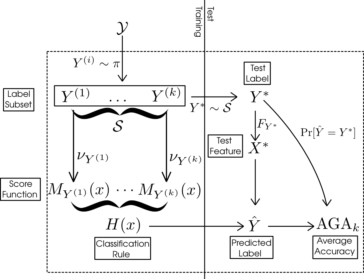
Figure 1: Average generalization accuracy: A diagram of the random quantities underlying the average generalization accuracy for $k$ labels ($\text{AGA}_{k}$). At the training stage (left), a set of $k$ labels $\mathcal{S}$ is sampled from the prior $\pi$, and score functions are trained from examples for these classes. At the test stage (right), one true class $Y^{*}$ is sampled uniformly from $\mathcal{S}$, as well as a test example $X^{*}$. $\text{AGA}_{k}$ measures the expected accuracy over these random variables.

2.1 Marginal Classifier

In our analysis, we do not want the classifier to rely too strongly on complicated interactions between the labels in the set. We therefore propose the following property of marginal separability for classification models:

Definition 1.

The classifier $H(x)$ is called a marginal classifier if the score function $M_{y^{(i)}}(x)$ only depends on the label $y^{(i)}$ and the class training set $X_{j,train}^{(i)}$; that is, for some function $g$,

$$M_{y^{(i)}}(x)=g(x;y^{(i)},X_{1,train}^{(i)},...,X_{r_{train},train}^{(i)}).$$

This means that the score function for $y^{(i)}$ does not depend on other labels $y^{(j)}$ or their training samples. Therefore, each $M_{y}$ can be considered to have been drawn from a distribution $\nu_{y}$. Classes “compete” only through selecting the highest score, but not in constructing the score functions. The operation of a marginal classifier is illustrated in Figure 2.

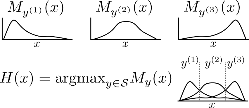
Figure 2: Classification rule: Top: Score functions for three classes in a one-dimensional example space. Bottom: The classification rule chooses between $y^{(1)},y^{(2)}$ or $y^{(3)}$ by choosing the maximal score function.

The marginal property allows us to prove strong results about the accuracy of the classifier under i.i.d. sampling assumptions.

Comments:

1. If $H$ is a marginal classifier then $M_{Y^{(i)}}$ is independent of $Y^{(j)}$ and $M_{Y^{(j)}}$ for $i\neq j$.

2. Estimated Bayes classifiers are primary examples of marginal classifiers. Let $\hat{f_{y}}$ be a density estimate of the example distribution under label $y$ obtained from the empirical distribution $\hat{F_{y}}$. Then, we can use the estimated density to produce the score functions:

   $$M^{EB}_{y}(x)=\log(\hat{f_{y}}(x)).$$

   The resulting empirical approximation for the Bayes classifier would be

   $$H^{EB}(x)=\text{argmax}_{Y\in\mathcal{S}}(M^{EB}_{Y}(x)).$$

3. Both Quadratic Discriminant Analysis (QDA) and na ive Bayes classifiers can be seen as specific instances of an estimated Bayes classifier. For QDA, the score function is given by

   $$m_{y}^{QDA}(x)=-(x-\mu(\hat{F}_{y}))^{T}\Sigma(\hat{F}_{y})^{-1}(x-\mu(\hat{F}_{y}))-\log\det(\Sigma(\hat{F}_{y})),$$

   where $\mu(F)=\int ydF(y)$ and $\Sigma(F)=\int(y-\mu(F))(y-\mu(F))^{T}dF(y)$. In Naive Bayes, the score function is

   $$m^{NB}_{y}(x)=\sum_{j=1}^{p}\log\hat{f}_{y,j}(x),$$

   where $\hat{f}_{y,j}$ is a density estimate for the $j$-th component of $\hat{F}_{y}$.

4. For some classifiers, $M_{y}$ is a deterministic function of $y$ (and therefore $\nu_{y}$ is degenerate). A prime example is when there exist fixed or pre-trained embeddings $g,\tilde{g}$ that map labels $y$ and examples $x$ into $R^{p}$. Then

   $$M_{y}^{embed}=-\|g(y)-\tilde{g}(x)\|_{2}.$$ (2)

5. There are many classifiers which do not satisfy the marginal property, such as multinomial logistic regression, multilayer neural networks, decision trees, and k-nearest neighbors.

Notational remark. Henceforth, we shall relax the assumption that the classifier $H(x)$ is based on a training set. Instead, we assume that there exist score functions $\{M_{Y^{(i)}}\}_{i=1}^{k}$ associated with the random label set $\{Y^{(i)}\}_{i=1}^{k}$, and that the score functions $M_{Y^{(i)}}$ are independent of the test set. The classifier $H(x)$ is marginal if and only if $M_{Y^{(i)}}$ are independent of both $Y^{(j)}$ and $M_{Y^{(j)}}$ for $j\neq i$.

2.2 Estimation of Average Accuracy

Before tackling extrapolation, it is useful to discuss a simpler task of generalizing accuracy results when the target set is not larger than the source set. Suppose we have test data for a classification task with $k_{1}$ classes. That is, we have a label set $\mathcal{S}_{k_{1}}=\{y^{(i)}\}_{i=1}^{k_{1}}$ and its associated set of score functions $M_{y^{(i)}}$, as well as test observations $(x_{1}^{(i)},\ldots,x_{r}^{(i)})$ for $i=1,\ldots,k_{1}$. What would be the predicted accuracy for a new randomly sampled set of $k_{2}\leq k_{1}$ labels?

Note that $\text{AGA}_{k_{2}}$ is the expected value of the accuracy on the new set of $k_{2}$ labels. Therefore, any unbiased estimator of $\text{AGA}_{k_{2}}$ will be an unbiased predictor for the accuracy on the new set.

Let us start with the case $k_{2}=k_{1}=k$. For each test observation $x_{j}^{(i)}$, define the ranks of the candidate classes $\ell=1,\ldots,k$ by

$$R_{j}^{i,\ell}=\sum_{s=1}^{k}I\{m_{y^{(\ell)}}(x_{j}^{(i)})\geq m_{y^{(s)}}(x_{j}^{(i)})\}.$$

The test accuracy is the fraction of observations for which the correct class also has the highest rank

$$\text{TA}_{k}=\frac{1}{rk}\sum_{i=1}^{k}\sum_{j=1}^{r}I\{R_{j}^{i,i}=k\}.$$ (3)

Taking expectations over both the test set and the random labels, the expected value of the test accuracy is $\text{AGA}_{k}$. Therefore, in this special case, $\text{TA}_{k}$ provides an unbiased estimator for $\text{AGA}_{k_{2}}$.

Next, let us consider the case where $k_{2}<k_{1}$. Consider label set $\mathcal{S}_{k_{2}}$ obtained by sampling $k_{2}$ labels uniformly without replacement from $\mathcal{S}_{k_{1}}$. Since $\mathcal{S}_{k_{2}}$ is unconditionally an i.i.d. sample from the population of labels $\pi$, the test accuracy of $\mathcal{S}_{k_{2}}$ is an unbiased estimator of $\text{AGA}_{k_{2}}$. However, we can get a better unbiased estimate of $\text{AGA}_{k_{2}}$ by averaging over all the possible subsamples $\mathcal{S}_{k_{2}}\subset\mathcal{S}_{k_{1}}$. This defines the average test accuracy over subsampled tasks, $\text{ATA}_{k_{2}}$.

Remark. Naïvely, computing $\text{ATA}_{k_{2}}$ requires us to train and evaluate ${k_{1}}\choose{k_{2}}$ classification rules. However, for marginal classifiers, retraining the classifier is not necessary. Looking at the rank $R_{j}^{i,i}$ of the correct label $i$ for $x_{j}^{(i)}$, allows us to determine how many subsets $\mathcal{S}_{2}$ will result in a correct classification. Specifically, there are $R_{j}^{i,i}-1$ labels with a lower score than the correct label $i$. Therefore, as long as one of the classes in $\mathcal{S}_{2}$ is $i$, and the other $k_{2}-1$ labels are from the set of $R_{j}^{i,i}-1$ labels with lower score than $i$, the classification of $x_{j}^{(i)}$ will be correct. This implies that there are ${R_{j}^{i,i}-1}\choose{k_{2}-1}$ such subsets $\mathcal{S}_{2}$ where $x_{j}^{(i)}$ is classified correctly, and therefore the average test accuracy for all ${k_{1}}\choose{k_{2}}$ subsets $\mathcal{S}_{2}$ is

$$\text{ATA}_{k_{2}}=\frac{1}{{{k_{1}}\choose{k_{2}}}}\frac{1}{rk_{2}}\sum_{i=1}^{k_{1}}\sum_{j=1}^{r}{{R_{j}^{i,i}-1}\choose{k_{2}-1}}.$$ (4)

2.3 Toy Example: Bivariate Normal

Let us illustrate these ideas using a toy example. Let $(Y,X)$ have a bivariate normal joint distribution,

$$(Y,X)\sim N\left(\begin{pmatrix}0\\ 0\end{pmatrix},\begin{pmatrix}1&\rho\\ \rho&1\end{pmatrix}\right),$$

as illustrated in Figure 3(a). Therefore, for a given randomly drawn label $Y$, the conditional distribution of $X$ for that label is univariate normal with mean $\rho Y$ and variance $1-\rho^{2}$,

$$X|Y=y\sim N(\rho Y,1-\rho^{2}).$$

Supposing we draw $k=3$ labels $\{y_{1},y_{2},y_{3}\}$, the classification problem will be to assign a test instance $X^{*}$ to the correct label. The test instance $X^{*}$ would be drawn with equal probability from one of three conditional distributions $X|Y=y^{(i)}$, as illustrated in Figure 3(b, top). The Bayes rule assigns $X^{*}$ to the class with the highest density $p(x|y_{i})$, as illustrated by Figure 3(b, bottom): it is therefore a marginal classifier, with score function

$$M_{y^{(i)}}(x)=\log(p(x|y^{(i)}))=-\frac{(x-\rho y)^{2}}{2(1-\rho^{2})}+\text{const.}$$

Joint distribution of $(X,Y)$	Problem instance with $k=3$
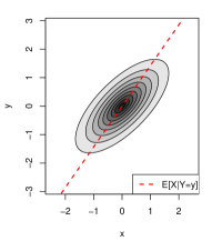
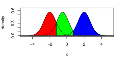
(a)	(b)

Figure 3: Toy example: Left: The joint distribution of $(X,Y)$ is bivariate normal with correlation $\rho=0.7$. Right: A typical classification problem instance from the bivariate normal model with $k=3$ classes. (Top): the conditional density of $X$ given label $Y$, for $Y=\{y^{(1)},y^{(2)},y^{(3)}\}$. (Bottom): the Bayes classification regions for the three classes.

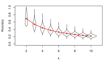
Figure 4: Generalization accuracy for toy example: The distribution of the generalization accuracy for $k=2,3,\ldots,10$ for the bivariate normal model with $\rho=0.7$. Circles indicate the average generalization accuracy $\text{AGA}_{k}$; the red curve is the theoretically computed average accuracy.

3 Extrapolation

For this model, the generalization accuracy of the Bayes rule for any label set $\{y^{(1)},\ldots,y^{(k)}\}$ is given by

$$\text{GA}_{k}(y_{1},\ldots,y_{k}) =\frac{1}{k}\sum_{i=1}^{k}\Pr_{X\sim p(x|y_{i})}[p(X|y_{i})=\max_{j=1}^{k}p(X|y_{j})]$$

$$=\frac{1}{k}\sum_{i=1}^{k}\Phi\left(\frac{y^{[i+1]}-y^{[i]}}{2\sqrt{1-\rho^{2}}}\right)-\Phi\left(\frac{y^{[i-1]}-y^{[i]}}{2\sqrt{1-\rho^{2}}}\right),$$

where $\Phi$ is the standard normal cdf, $y^{[1]}<\cdots<y^{[k]}$ are the sorted labels, $y^{[0]}=-\infty$ and $y^{[k+1]}=\infty$. We numerically computed $\text{GA}_{k}(Y_{1},\ldots,Y_{k})$ for randomly drawn labels $Y_{1},\ldots,Y_{k}\stackrel{{\scriptstyle iid}}{{\sim}}N(0,1)$, and the distributions of $\text{GA}_{k}$ for $k=2,\ldots,10$ are illustrated in Figure 4. The mean of the distribution of $\text{GA}_{k}$ is the $k$-class average accuracy, $\text{AGA}_{k}$. The theory presented in the next section deals with how to analyze the average accuracy $\text{AGA}_{k}$ as a function of $k$.

The section is organized as follows. We begin by introducing an explicit formula for the average accuracy $\text{AGA}_{k}$. The formula reveals that $\text{AGA}_{k}$ is determined by moments of a one-dimensional function ${D}(u)$. Using this formula, we can estimate ${D}(u)$ using subsampled accuracies. These estimates allow us to extrapolate the average generalization accuracy to an arbitrary number of labels.

The result of our analysis is to expose the average accuracy $\text{AGA}_{k}$ as the weighted average of a function ${D}(u)$, where ${D}(u)$ is independent of $k$, and where $k$ only changes the weighting. The result is stated as follows.

Theorem 1.

Suppose $\pi$, $\{F_{y}\}_{y\in\mathcal{Y}}$, and score functions $M_{y}$ satisfy the tie-breaking condition. Then, there exists a cumulative distribution function ${D}(u)$ defined on the interval $[0,1]$ such that

$$\text{AGA}_{k}=1-(k-1)\int{D}(u)u^{k-2}du.$$ (5)

The tie-breaking allows us to neglect specifying the case when margins are tied.

Definition 2.

Tie-breaking condition: for all $x\in\mathcal{X}$, $M_{Y}(x)\neq M_{Y^{\prime}}(x)$ with probability one for $Y,Y^{\prime}$ independently drawn from $\pi$.

In practice, one can simply break ties randomly, which is mathematically equivalent to adding a small amount of random noise $\epsilon$ to the function $\mathcal{M}$.

3.1 Analysis of Average Accuracy

For the following discussion, we often consider a random label with its associated score function and example vector. Explicitly, this sampling can be written:

$$Y\sim\pi,\,M_{Y}|Y\sim\nu_{Y},\,X|Y\sim F_{Y}.$$

Similarly we use $(Y^{\prime},M_{Y^{\prime}},X^{\prime})$ and $(Y^{*},M_{Y^{*}},X^{*})$ for two more triplets with independent and identical distributions. Specifically, $X^{*}$ will typically note the test example, and therefore $Y^{*}$ the true label and $M_{Y^{*}}$ its score function.

The function ${D}$ is related to a favorability function. Favorability measures the probability that the score for the example $x^{*}$ is going to be maximized by a particular score function $m_{y}$, compared to a random competitor $M_{Y^{\prime}}$. Formally, we write

$$U_{x^{*}}(m_{y})=\Pr[m_{y}(x^{*})>M_{Y^{\prime}}(x^{*})].$$ (6)

Note that for fixed example $x^{*}$, favorability is monotonically increasing in $m_{y}(x^{*})$. If $m_{y}(x^{*})>m_{y^{\dagger}}(x^{*})$, then $U_{x^{*}}(y)>U_{x^{*}}(y^{\dagger})$, because the event $\{m_{y}(x^{*})>M_{Y^{\prime}}(x^{*})\}$ contains the event $\{m_{y^{\dagger}}(x^{*})>M_{Y^{\prime}}(x^{*})\}$.

Therefore, given labels $y^{(1)},\ldots,y^{(k)}$ and test instance $x^{*}$, we can think of the classifier as choosing the label with the greatest favorability:

$$\hat{y}=\text{argmax}_{y^{(i)}\in\mathcal{S}}m_{y^{(i)}}(x^{*})=\text{argmax}_{y^{(i)}\in\mathcal{S}}U_{x^{*}}(m_{y^{(i)}}).$$

Furthermore, via a conditioning argument, we see that this is still the case even when the test instance and labels are random:

$$\hat{Y}=\text{argmax}_{Y^{(i)}\in\mathcal{S}}M_{Y^{(i)}}(X^{*})=\text{argmax}_{Y^{(i)}\in\mathcal{S}}U_{X^{*}}(M_{Y^{(i)}}).$$

The favorability takes values between 0 and 1, and when any of its arguments are random, it becomes a random variable with a distribution supported on $[0,1]$. In particular, we consider the following two random variables:

• the incorrect-label favorability $U_{x^{*}}(M_{Y})$ between a given fixed test instance $x^{*}$, and the score function of a random incorrect label $M_{Y}$, and

• the correct-label favorability $U_{X^{*}}(M_{Y^{*}})$ between a random test instance $X^{*}$, and the score function of the correct label, $M_{Y^{*}}$.

3.1.1 Incorrect-Label Favorability

The incorrect-label favorability can be written explicitly as

$$U_{x^{*}}(M_{Y})=\Pr[M_{Y}(x^{*})>M_{Y^{\prime}}(x^{*})|M_{Y}].$$ (7)

Note that $M_{Y}$ and $M_{Y^{\prime}}$ are identically distributed, and are both are unrelated to $x^{*}$ that is fixed. This leads to the following result:

Lemma 1.

Under the tie-breaking condition, the incorrect-label favorability $U_{x^{*}}(M_{Y})$ is uniformly distributed for any $x^{*}\in\mathcal{X}$, meaning

$$\Pr[U_{x^{*}}(M_{Y})\leq u]=u$$ (8)

for all $u\in[0,1].$

Proof.

Write $U_{x^{*}}(M_{Y})=\Pr[Z>Z^{\prime}|Z]$, where $Z=M_{Y}(x)$ and $Z^{\prime}=M_{Y^{\prime}}(x)$ for $Y,Y^{\prime}\stackrel{{\scriptstyle i.i.d.}}{{\sim}}\pi$. The tie-breaking condition implies that $\Pr[Z=Z^{\prime}]=0$. Now observe that for independent random variables $Z,Z^{\prime}$ with $Z\stackrel{{\scriptstyle D}}{{=}}Z^{\prime}$ and $\Pr[Z=Z^{\prime}]=0$, the conditional probability $\Pr[Z>Z^{\prime}|Z]$ is uniformly distributed. ∎

3.1.2 Correct-Label Favorability

The correct-label favorability is

$$U^{*}=U_{X^{*}}(M_{Y^{*}})=\Pr[M_{Y^{*}}(X^{*})>M_{Y^{\prime}}(X^{*})|Y^{*},M_{Y^{*}},X^{*}].$$ (9)

The distribution of $U^{*}$ will depend on $\pi$, $\{F_{y}\}_{y\in\mathcal{S}}$ and $\{\nu_{y}\}_{y\in\mathcal{S}}$, and generally cannot be written in a closed form. However, this distribution is central to our analysis–indeed, we will see that the function ${D}$ appearing in theorem 1 is defined as the cumulative distribution function of $U^{*}$.

The special case of $k=2$ shows the relation between the distribution of $U^{*}$ and the average generalization accuracy, $\text{AGA}_{2}$. In the two-class case, the average generalization accuracy is the probability that a random correct label score function gives a larger value than a random distractor:

$$\text{AGA}_{2}=\Pr[M_{Y^{*}}(X^{*})>M_{Y^{\prime}}(X^{*})].$$

where $Y^{*}$ is the correct label, and $Y^{\prime}$ is a random incorrect label. If we condition on $Y^{*}$, $M_{Y^{*}}$ and $X^{*}$, we get

$$\text{AGA}_{2}=\textbf{E}[\Pr[M_{Y^{*}}(X^{*})>M_{Y^{\prime}}(X^{*})|Y^{*},M_{Y^{*}},X^{*}]].$$

Here, the conditional probability inside the expectation is the correct-label favorability. Therefore,

$$\text{AGA}_{2}=\textbf{E}[U^{*}]=\int{D}(u)du,$$

where ${D}(u)$ is the cumulative distribution function of $U^{*}$, ${D}(u)=\Pr[U^{*}\leq u]$. Theorem 1 extends this to general $k$; we now give the proof.

Proof.

Without loss of generality, suppose that the true label is $Y^{*}$ and the incorrect labels are $Y^{(1)},\ldots,Y^{(k-1)}$. We have

$$\text{AGA}_{k}=\Pr[M_{Y^{*}}(X^{*})>\max_{i=1}^{k-1}M_{Y^{(i)}}(X^{*})]=\Pr[U^{*}>\max_{i=1}^{k-1}U_{X^{*}}(M_{Y^{(i)}})],$$

recalling that $U^{*}=U_{X^{*}}(M_{Y^{*}})$. Now, if we condition on $X^{*}=x^{*}$, $Y^{*}=y^{*}$ and $M_{Y^{*}}=m_{y^{*}}$, then the random variable $U^{*}$ becomes fixed, with value

$$u^{*}=U_{x^{*}}(m_{y^{*}}).$$

Therefore,

$$\text{AGA}_{k} =\textbf{E}[\Pr[U^{*}>\max_{i=1}^{k-1}U_{X^{*}}(M_{Y^{(i)}})|X^{*}=x^{*},Y^{*}=y^{*},M_{Y^{*}}=m_{y^{*}}]]$$

$$=\textbf{E}[\Pr[U^{*}>\max_{i=1}^{k-1}U_{X^{*}}(M_{Y^{(i)}})|X^{*}=x^{*},U^{*}=u^{*}]].$$

Now define $U_{max,k-1}=\max_{i=1}^{k-1}U_{X^{*}}(M_{Y^{(i)}})$. Since by Lemma 1, $U_{X^{*}}(M_{Y^{(i)}})$ are i.i.d. uniform conditional on $X^{*}=x^{*}$, we know that

$$U_{max,k-1}|X^{*}=x^{*}\sim\text{Beta}(k-1,1).$$ (10)

Furthermore, $U_{max,k-1}$ is independent of $U^{*}$ conditional on $X^{*}$. Therefore, the conditional probability can be computed as

$$\Pr[U^{*}>U_{max,k-1}|X^{*}=x^{*},U^{*}=u^{*}]=\int_{u^{*}}^{1}(k-1)u^{k-2}du.$$

Consequently,

$$\text{AGA}_{k} =\textbf{E}[\Pr[U^{*}>\max_{i=1}^{k-1}U_{X^{*}}(M_{Y^{(i)}})|X^{*}=x^{*},U^{*}=u^{*}]]$$ (11)

$$=\textbf{E}[\int_{0}^{U^{*}}(k-1)u^{k-2}du|U^{*}=u^{*}]$$ (12)

$$=\textbf{E}[\int_{0}^{1}I\{u\leq U^{*}\}(k-1)u^{k-2}du]$$ (13)

$$=(k-1)\int_{0}^{1}\Pr[U^{*}\geq u]u^{k-2}du$$ (14)

$$=1-(k-1)\int_{0}^{1}\Pr[U^{*}\leq u]u^{k-2}du.$$ (15)

By defining ${D}(u)$ as the cumulative distribution function of $U^{*}$ on $[0,1]$,

$${D}(u)=\Pr[U_{X^{*}}(M_{Y^{*}})\leq u],$$ (16)

and substituting this definition into (15), we obtain the identity (5). ∎

Theorem 1 expresses the average accuracy as a weighted integral of the function ${D}(u)$. Essentially, this theoretical result allows us to reduce the problem of estimating $\text{AGA}_{k}$ to one of estimating $D(u)$. But how shall we estimate $D(u)$ from data? We propose using non-parametric regression for this purpose in Section 3.3.

3.2 Favorability and Average Accuracy for the Toy Example

Recall that for the toy example from Section 2.3, the score function $M_{y}$ was a non-random function of $y$ that measures the distance between $x$ and $\rho y$

$$M_{y}(x^{*})=\log(p(x^{*}|y))=-\frac{(x^{*}-\rho y)^{2}}{2(1-\rho^{2})}.$$

For this model, the favorability function $U_{x^{*}}(m_{y})$ compares the distance between $x^{*}$ and $\rho y$ to the distance between $x^{*}$ and $\rho Y^{\prime}$ for a randomly chosen distractor $Y^{\prime}\sim N(0,1)$:

$$U_{x^{*}}(m_{y}) =\Pr[|\rho y-x^{*}|>|\rho Y^{\prime}-x^{*}|]$$

$$=\Phi\left(\frac{x^{*}+|\rho y-x^{*}|}{\rho}\right)-\Phi\left(\frac{x^{*}-|\rho y-x^{*}|}{\rho}\right),$$

where $\Phi$ is the standard normal cumulative distribution function. Figure 5(a) illustrates the level sets of the function $U_{x^{*}}(m_{y})$. The highest values of $U_{x^{*}}(m_{y})$ are near the line $x^{*}=\rho y$ corresponding to the conditional mean of $X|Y$, and as one moves farther from the line, $U_{x^{*}}(m_{y})$ decays. Note, however, that large values of $x^{*}$ and $y$ (with the same sign) result in larger values of $U_{x^{*}}(m_{y})$ since it becomes unlikely for $Y^{\prime}\sim N(0,1)$ to exceed $Y=y$.

Using the formula above, we can calculate the correct-label favorability $U^{*}=U_{X^{*}}(M_{Y^{*}})$ and its cumulative distribution function ${D}(u)$. The function ${D}$ is illustrated in Figure 5(b) for the current example with $\rho=0.7$. The red curve in Figure 4 was computed using the formula

$$\text{AGA}_{k}=1-(k-1)\int{D}(u)u^{k-2}du.$$

It is illuminating to consider how the average accuracy curves and the ${D}(u)$ functions vary as we change the parameter $\rho$. Higher correlations $\rho$ lead to higher accuracy, as seen in Figure 6(a), where the accuracy curves are shifted upward as $\rho$ increases from 0.3 to 0.9. The favorability $U_{x^{*}}(m_{y})$ tends to be higher on average as well, which leads to lower values of the cumulative distribution function–as we see in Figure 6(b), where the function ${D}(u)$ becomes smaller as $\rho$ increases.

$U_{x}^{*}(M_{y})$ for $\rho=0.7$	$D(u)$ for $\rho=0.7$

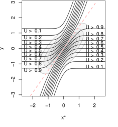
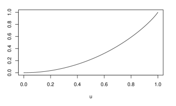
Figure 5: Favorability for toy example: Left: The level curves of the function $U_{x^{*}}(M_{y})$ in the bivariate normal model with $\rho=0.7$. Right: The function ${D}(u)$ gives the cumulative distribution function of the random variable $U_{X^{*}}(M_{Y})$.

$D(u)$	Average Accuracy

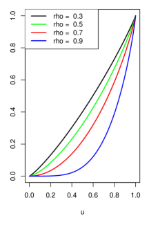
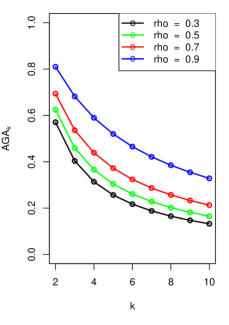
Figure 6: Average accuracy with different $\rho$’s: Left: The average accuracy $\text{AGA}_{k}$. Right: ${D}(u)$ function for the bivariate normal model with $\rho\in\{0.3,0.5,0.7,0.9\}$.

3.3 Estimation

Next, we discuss how to use data from smaller classification tasks to extrapolate average accuracy. Assume that we have data from a $k_{1}$-class random classification task, and would like to estimate the average accuracy $\text{AGA}_{k_{2}}$ for $k_{2}>k_{1}$ classes. Our estimation method will use the $k$-class average test accuracies, $\text{ATA}_{2},...,\text{ATA}_{k_{1}}$ (see Eq 4), for its inputs.

The key to understanding the behavior of the average accuracy $\text{AGA}_{k}$ is the function ${D}$. We adopt a linear model

$${D}(u)=\sum_{\ell=1}^{m}\beta_{\ell}h_{\ell}(u),$$ (17)

where $h_{\ell}(u)$ are known basis functions, and $\beta_{\ell}$ are the linear coefficients to be estimated. Since our proposed method is based on the linearity assumption (17), we refer to it as ClassExReg, meaning Classification Extrapolation using Regression.

Conveniently, $\text{AGA}_{k}$ can also be expressed in terms of the $\beta_{\ell}$ coefficients. If we plug in the assumed linear model (17) into the identity (5), then we get

$$1-\text{AGA}_{k} =(k-1)\int{D}(u)u^{k-2}du$$ (18)

$$=(k-1)\int_{0}^{1}\sum_{\ell=1}^{m}\beta_{\ell}h_{\ell}(u)u^{k-2}du$$ (19)

$$=\sum_{\ell=1}^{m}\beta_{\ell}H_{\ell,k},$$ (20)

where

$$H_{\ell,k}=(k-1)\int_{0}^{1}h_{\ell}(u)u^{k-2}du.$$ (21)

The constants $H_{\ell,k}$ are moments of the basis function $h_{\ell}$. Note that $H_{\ell,k}$ can be precomputed numerically for any $k\geq 2$.

Now, since the test accuracies $\text{ATA}_{k}$ are unbiased estimates of $\text{AGA}_{k}$, this implies that the regression estimate

$$\hat{\beta}=\text{argmin}_{\beta}\sum_{k=2}^{k_{1}}\left((1-\text{ATA}_{k})-\sum_{\ell=1}^{m}\beta_{\ell}H_{\ell,k}\right)^{2},$$

is unbiased for $\beta$. The estimate of $\text{AGA}_{k_{2}}$ is similarly obtained from (20), via

$$\widehat{\text{AGA}_{k_{2}}}=1-\sum_{\ell=1}^{m}\hat{\beta}_{\ell}H_{\ell,k_{2}}.$$ (22)

3.4 Model Selection

Accurate extrapolation using ClassExReg depends on a good fit between the linear model (17) and the true discriminability function $D(u)$. However, since the function $D(u)$ depends on the unknown joint distribution of the data, it makes sense to let the data help us choose a good basis $\{h_{u}\}$ from a set of candidate bases.

Let $B_{1},\ldots,B_{s}$ be a set of candidate bases, with $B_{i}=\{h_{u}^{(i)}\}_{u=1}^{m_{i}}$. Ideally, we would like our model selection procedure to choose the $B_{i}$ that obtains the best root-mean-squared error (RMSE) on the extrapolation from $k_{1}$ to $k_{2}$ classes. As an approximation, we estimate the RMSE of extrapolation from $\frac{k_{1}}{2}$ source classes to $k_{1}$ target classes, by means of the “bootstrap principle.” This amounts to a resampling-based model selection approach, where we perform extrapolations from $k_{0}=\lfloor\frac{k_{1}}{2}\rfloor$ classes to $k_{1}$ classes, and evaluate methods based on how closely the predicted $\widehat{\text{ABA}}_{k_{1}}$ matches the test accuracy $\text{ATA}_{k_{1}}$. To elaborate, our model selection procedure is as follows.

1. For $\ell=1,\ldots,L$ resampling steps:

   1. Subsample $\mathcal{S}_{k_{0}}^{(\ell)}$ from $\mathcal{S}_{k_{1}}$ uniformly with replacement.

   2. Compute average test accuracies $\text{ATA}_{2}^{(\ell)},\ldots,\text{ATA}_{k_{0}}^{(\ell)}$ from the subsample $\mathcal{S}_{k_{0}}^{(\ell)}$.

   3. For each candidate basis $B_{i}$, with $i=1,\ldots,s$:

      1. Compute $\hat{\beta}^{(i,\ell)}$ by solving the least-squares problem

         $$\hat{\beta}^{(i,\ell)}=\text{argmin}_{\beta}\sum_{k=2}^{k_{0}}\left((1-\text{ATA}_{k}^{(\ell)})-\sum_{j=1}^{m_{i}}\beta_{j}H_{j,k}^{(i)}\right)^{2}.$$

      2. Estimate $\widehat{\text{AGA}}_{k_{1}}^{(i,\ell)}$ by

         $$\widehat{\text{AGA}}_{k_{1}}^{(i,\ell)}=\sum_{\ell=1}^{m_{i}}\hat{\beta}_{j}^{(i,\ell)}H_{j,k_{1}}^{(i)}.$$

2. Select the basis $B_{i^{*}}$ by

   $$i^{*}=\text{argmin}_{i=1}^{s}\sum_{\ell=1}^{L}(\widehat{\text{AGA}}_{k_{1}}^{(i,\ell)}-\text{ATA}_{k_{1}})^{2}.$$

3. Use the basis $B_{i^{*}}$ to extrapolate from $k_{1}$ classes (the full data) to $k_{2}$ classes.

4 Simulation Study

We ran simulations to check how the proposed extrapolation method, ClassExReg, performs in different settings. The results are displayed in Figure 7. We varied the number of classes $k_{1}$ in the source data set, the difficulty of classification, and the basis functions. We generated data according to a mixture of isotropic multivariate Gaussian distributions: labels $Y$ were sampled from $Y\sim N(0,I_{10})$, and the examples for each label sampled from $X|Y\sim N(Y,\sigma^{2}I_{10})$. The noise-level parameter $\sigma$ determines the difficulty of classification. Similarly to the real-data example, we consider a 1-nearest neighbor classifier, which is given a single training instance per class.

For the estimation, we use the model selection procedure described in section 3.4 to select the parameter $h$ of the “radial basis”

$$h_{\ell}(u)=\Phi\left(\frac{\Phi^{-1}(u)-t_{\ell}}{h}\right).$$

where $t_{\ell}$ are a set of regularly spaced knots which are determined by $h$ and the problem parameters. Additionally, we add a constant element to the basis, equivalent to adding an intercept to the linear model (17).

The rationale behind the radial basis is to model the density of $\Phi^{-1}(U^{*})$ as a mixture of gaussian kernels with variance $h^{2}$. To control overfitting, the knots are separated by at least a distance of $h/2$, and the largest knots have absolute value $\Phi^{-1}(1-\frac{1}{rk_{1}^{2}}).$ The size of the maximum knot is set this way since $rk_{1}^{2}$ is the number of ranks that are calculated and used by our method. Therefore, we do not expect the training data to contain enough information to allow our method to distinguish between more than $rk_{1}^{2}$ possible accuracies, and hence we set the maximum knot to prevent the inclusion of a basis element that has on average a higher mean value than $u=1-\frac{1}{rk_{1}^{2}}$. However, in simulations we find that the performance of the basis depends only weakly on the exact positioning and maximum size of the knots, as long as sufficiently large knots are included. As is the case throughout non-parametric statistics, the bandwidth $h$ is the most crucial parameter. In the simulation, we use a grid $h=\{0.1,0.2,\ldots,1\}$ for bandwidth selection.

4.1 Comparison to Kay

In their paper, Kay et al. (2008) proposed a method for extrapolating classification accuracy to a larger number of classes. The method depends on repeated kernel-density estimation (KDE) steps. Because the method is only briefly motivated in the original text, we present it in our notation.

For $k_{1}$ observed classes, let $m_{y^{(j)}}(x^{(i)}_{\ell})\,1\leq i,j\leq k_{1}$ be the observed score comparing feature vector of the $\ell$’th test example of the $i$’th class $x^{(i)}_{\ell}$ to the model trained for the $j$’th class $m_{y^{(j)}}$. For each feature-vector $x^{(i)}_{\ell}$, the density of wrong-class scores is estimated by smoothing the observed scores with a kernel function $K(\cdot,\cdot)$ with bandwidth $h$,

$$\hat{f}_{\ell}^{(i)}(m)=\frac{1}{k_{1}-1}\sum_{j\neq i}K_{h}(m_{y^{(j)}}(x^{(i)}_{\ell}),m).$$

An estimate of favorability for $x^{(i)}_{\ell}$ against a single competitor is obtained by integrating the density below the observed true score $m_{y^{(i)}}(x^{(i)}_{\ell})$,

$$acc_{2}(x_{\ell}^{(i)})=\int_{0}^{m_{y^{(i)}}(x^{(i)}_{\ell})}\hat{f}_{\ell}^{(i)}(m)dm,$$

and the probability of accurate classification against $K-1$ random competitors is $acc_{K}(x^{(i)}_{\ell})=(acc_{2}(x^{(i)}_{\ell}))^{K-1}$. The average of these probabilities is the estimate for generalization accuracy

$$\hat{AGA}_{K}^{(KDE)}=\frac{1}{k_{1}r}\sum_{i=1}^{k_{1}}\sum_{\ell=1}^{r}acc_{K}(x^{(i)}_{\ell}).$$

Note that the KDE method depends non-trivially on the smoothing bandwidth used in the density estimation step: when the kernel bandwidth is too small compared to the number of classes, the extrapolated accuracy will be upwardly biased. To see this, consider a feature vector $x^{(i)}_{\ell}$ that is correctly classified in the original class set. That is, $m_{y^{(i)}}(x^{(i)}_{\ell})>m_{y^{(j)}}(x^{(i)}_{\ell})$ for every $j\neq i$. If we use for $\hat{f}_{i}$ the unsmoothed empirical density, $acc_{2}(x^{(i)}_{\ell})=1$ and therefore $acc_{K}(x^{(i)}_{\ell})=1$ as well. The method relies on smoothing of each class to generate a the tail density that exceeds $m_{y^{(i)}}(x^{(i)}_{\ell})$, and therefore it is highly dependent on the choice of kernel bandwidth.

Kay et al. (2008) recommended using a Gaussian kernel, with the bandwidth chosen via pseudolikelihood cross-validation (Cao et al., 1994). In our simulation, we tested our own implementation of the KDE method, using the two methods for cross-validated KDE estimation provided in the stats package in the R statistical computing environment: biased cross-validation and unbiased cross-validation (Scott, 1992).

4.2 Simulation Results

We see in Figure 7 that ClassExReg and the KDE methods with unbiased and biased cross-validation (KDE-UCV, KDE-BCV) perform comparably in the Gaussian simulations. We studied how the difficulty of extrapolation relates to both the absolute size of the number of classes and the extrapolation factor $\frac{k_{2}}{k_{1}}$. Our simulation has two settings for $k_{1}=\{500,5000\}$, and within each setting we have extrapolations to 2 times, 4 times, 10 times, and 20 times the number of classes.

$k_{1}$	$k_{2}$	ClassExReg	KDE-BCV	KDE-UCV
500	1000	0.032 (0.001)	0.090 (0.001)	0.067 (0.001)
500	2000	0.044 (0.002)	0.088 (0.001)	0.059 (0.001)
500	5000	0.073 (0.004)	0.079 (0.001)	0.051 (0.001)
500	10000	0.098 (0.004)	0.076 (0.001)	0.045 (0.001)
5000	10000	0.009 (0.000)	0.038 (0.000)	0.028 (0.000)
5000	20000	0.015 (0.001)	0.028 (0.000)	0.019 (0.000)
5000	50000	0.032 (0.002)	0.035 (0.000)	0.053 (0.000)
5000	100000	0.054 (0.003)	0.065 (0.000)	0.086 (0.000)

Table 1: Maximum RMSE (se) across all signal-to-noise-levels in predicting $\text{TA}_{k_{2}}$ from $k_{1}$ classes in multivariate gaussian simulation. Standard errors were computed by nesting the maximum operation within the bootstrap, to properly account for the variance of a maximum of estimated means.

Within each problem setting defined by the number of source and target classes $(k_{1},k_{2})$, we use the maximum RMSE across all signal-to-noise settings to quantify the overall performance of the method, as displayed in Table 1.

The results also indicate that more accurate extrapolation appears to be possible for smaller extrapolation ratios $\frac{k_{2}}{k_{1}}$ and larger $k_{1}$. ClassExReg improves in worst-case RMSE when moving from $k_{1}=500$ to $k_{1}=5000$ while keeping the extrapolation factor fixed, most dramatically in the case $\frac{k_{2}}{k_{1}}=2$ when it improves from a maximum RMSE of $0.032\pm 0.001$ ($k_{1}=500$) to $0.009\pm 0.000$ ($k_{1}=5000$), which is 3.5-fold reduction in worst-case RMSE, but also benefiting from at least a 1.8-fold reduction in RMSE when going from the smaller problem to the larger problem in the other three cases.

The kernel-density method produces comparable results, but is seen to depend strongly on the choice of bandwidth selection: KDE-UCV and KDE-BCV show very different performance profiles, although they differ only in the method used to choose the bandwidth. Also, the KDE methods show significant estimation bias, as can be seen from Figure 8. This can be explained by the fact that the KDE method ignores the bias introduced by exponentiation. That is, even if $\hat{p}$ is an unbiased estimator of $p$, $\hat{p}^{k}$ may not be a very good estimate of $p^{k}$, since

$$p^{k}=\textbf{E}[\hat{p}]^{k}\neq\textbf{E}[\hat{p}^{k}].$$

unless $\hat{p}$ is a degenerate random variable (constant). Otherwise, for large $k$, $\hat{p}^{k}$ may be an extremely biased estimate of $p$. ClassExReg avoids this source of bias by estimating the $(k-1)$st moment of $D(u)$ directly. As we see in Figure 8, correcting for the bias of exponentiation helps greatly to reduce the overall bias. Indeed, while ClassExReg shows comparable bias for the 500 to 10000 extrapolation, the bias is very well-controlled in all of the $k_{1}=5000$ extrapolations.

Extrapolating from $k_{1}=500$
Predicting $\text{AGA}_{1000}$	Predicting $\text{AGA}_{2000}$
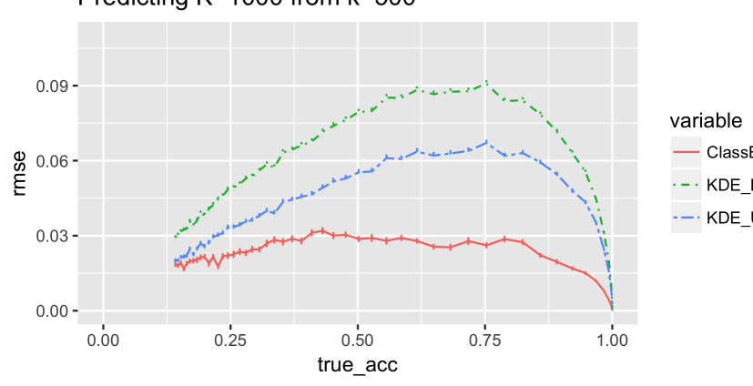
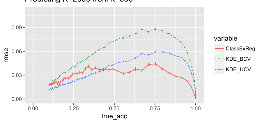
Predicting $\text{AGA}_{5000}$	Predicting $\text{AGA}_{10000}$
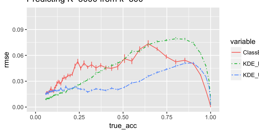
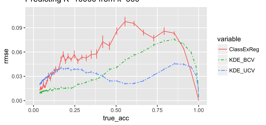
Extrapolating from $k_{1}=5000$
Predicting $\text{AGA}_{10000}$	Predicting $\text{AGA}_{20000}$
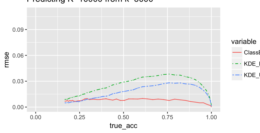
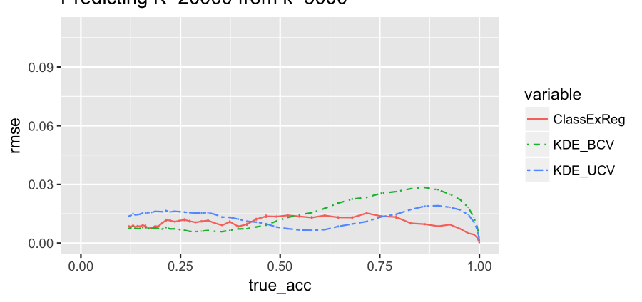
Predicting $\text{AGA}_{50000}$	Predicting $\text{AGA}_{100000}$

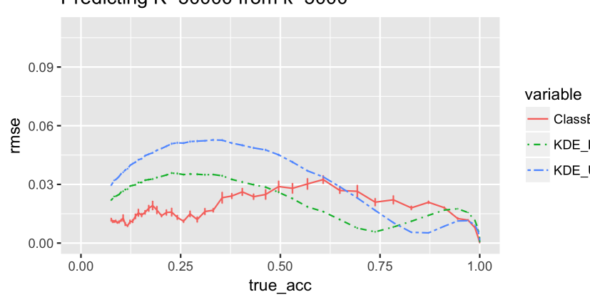
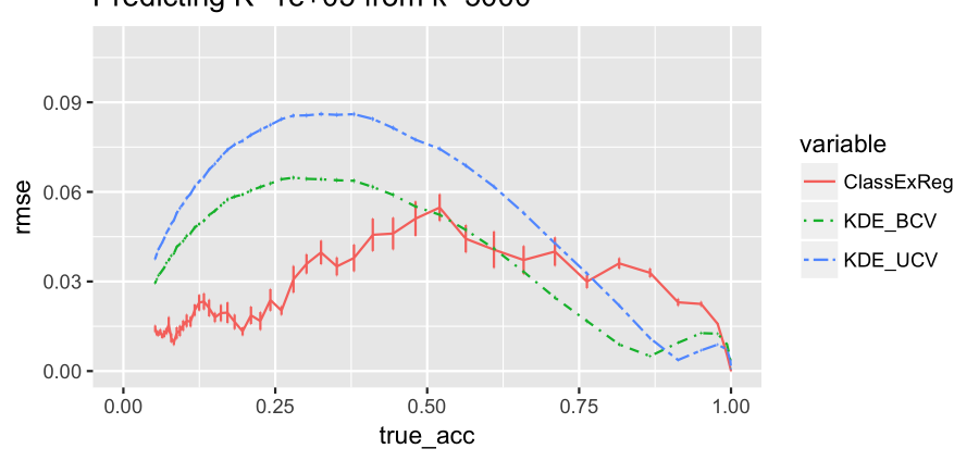
Figure 7: Simulation results (RMSE): Simulation study consisting of multivariate Gaussian $Y$ with nearest neighbor classifier. Prediction RMSE vs true $k_{2}$-class accuracy for ClassExReg with radial basis (ClassExReg), KDE-based methods with biased cross-validation (KDE_BCV) and unbiased cross-validation (KDE_UCV).

Extrapolating from $k_{1}=500$
Predicting $\text{AGA}_{2000}$	Predicting $\text{AGA}_{5000}$	Predicting $\text{AGA}_{10000}$
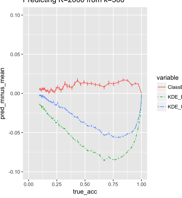
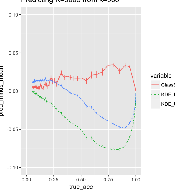
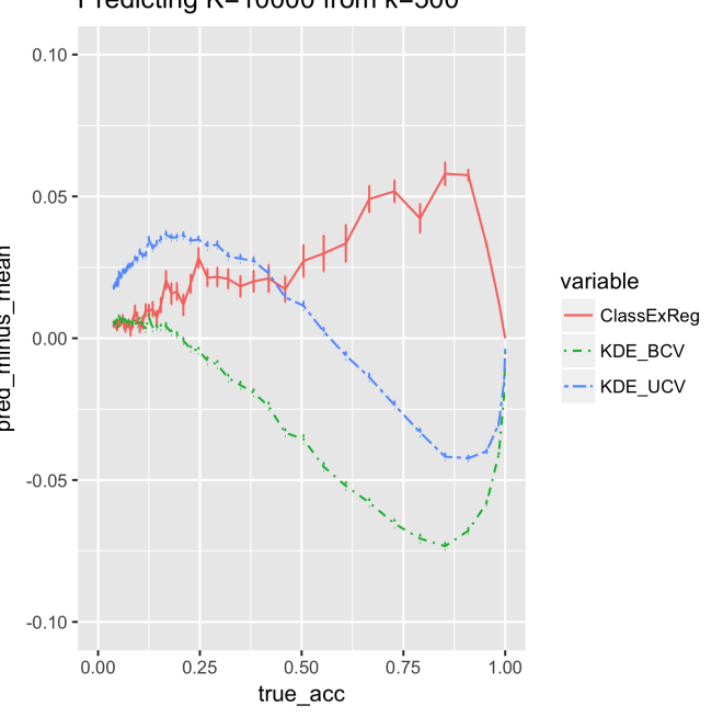
Extrapolating from $k_{1}=5000$
Predicting $\text{AGA}_{20000}$	Predicting $\text{AGA}_{50000}$	Predicting $\text{AGA}_{100000}$

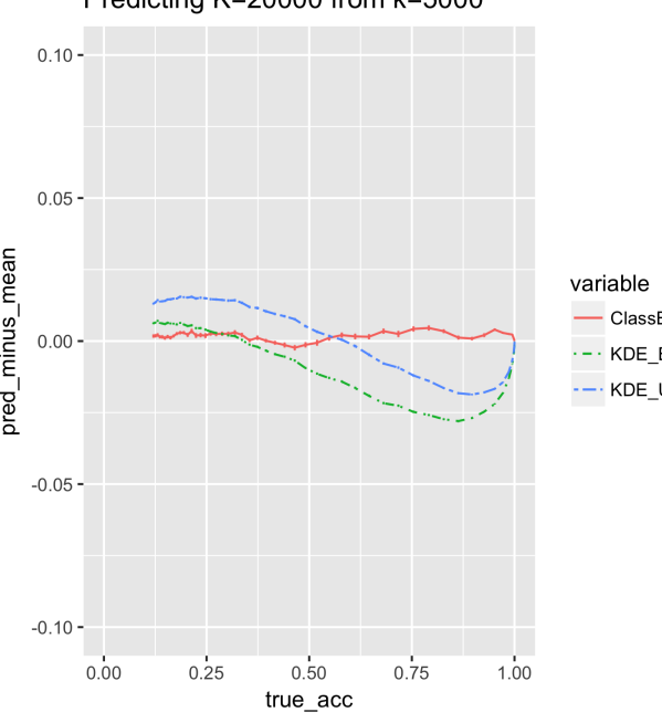
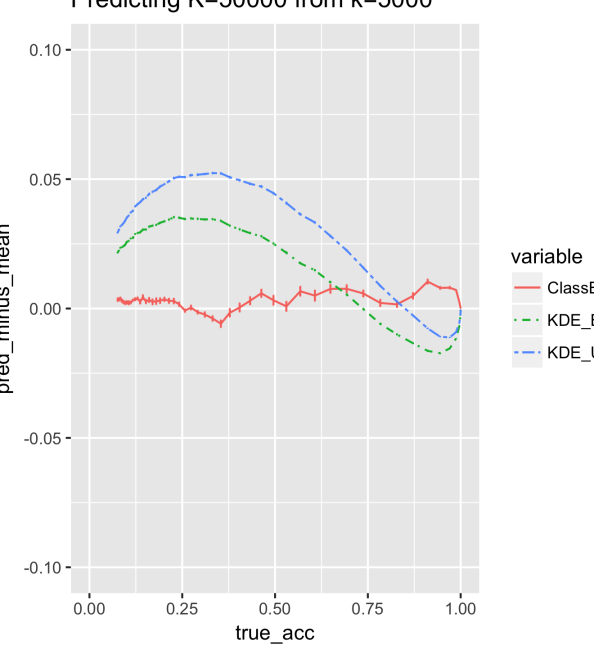
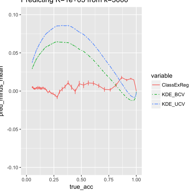
Figure 8: Simulation results (biases): Simulation study consisting of multivariate Gaussian $Y$ with nearest neighbor classifier. Bias (mean predicted minus true accuracy) vs true $k_{2}$-class accuracy for ClassExReg with radial basis (ClassExReg), KDE-based methods with biased cross-validation (KDE_BCV) and unbiased cross-validation (KDE_UCV).

5 Experimental Evaluation

We demonstrate the extrapolation of average accuracy in two data examples: (i) predicting the accuracy of a face recognition on a large set of labels from the system’s accuracy on a smaller subset, and (ii) extrapolating the performance of various classifiers on an optical character recognition (OCR) problem in the Telugu script, which has over 400 glyphs.

The face-recognition example takes data from the “Labeled Faces in the Wild” data set (Huang et al. (2007)), where we selected the 1672 individuals with at least 2 face photos. We form a data set consisting of photo-label pairs $(x_{j}^{(i)},y^{(i)})$ for $i=1,\ldots,1672$ and $j=1,2$ by randomly selecting 2 face photos for each individual. We used the OpenFace (Amos et al. (2016)) embedding for feature extraction. In order to identify a new photo $x^{*}$, we obtain the feature vector $g(x^{*})$ from the OpenFace network, and guess the label $\hat{y}$ with the minimal Euclidean distance between $g(y^{(i)})$ and $g(x^{*})$, which implies a score function

$$M_{y^{(i)}}(x^{*})=-||g(x_{1}^{(i)})-g(x^{*})||^{2}.$$

In this way, we can compute the test accuracy on all 1672 classes, $\text{TA}_{1672}$, but we also subsample $k_{1}=\{100,200,400\}$ classes in order to extrapolate from $k_{1}$ to 1672 classes.

Label		Training		Test
$y^{(1)}$=Amelia	$x_{1}^{(1)}=$	$x_{2}^{(1)}=$	$x_{3}^{(1)}=$	$x_{*}^{(1)}=$
$y^{(2)}$=Jean-Pierre	$x_{1}^{(2)}=$	$x_{2}^{(2)}=$	$x_{3}^{(2)}=$	$x_{*}^{(2)}=$
$y^{(3)}$=Liza	$x_{1}^{(3)}=$	$x_{2}^{(3)}=$	$x_{3}^{(3)}=$	$x_{4}^{(3)}=$
$y^{(4)}$=Patricia	$x_{1}^{(4)}=$	$x_{2}^{(4)}=$	$x_{3}^{(4)}=$	$x_{4}^{(4)}=$

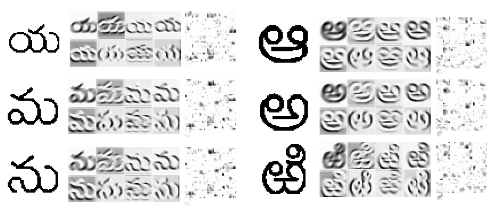
Figure 9: Face recognition setup (top): Examples of labels and features from the Labeled Faces in the Wild data set. Telugu OCR (bottom): exemplars from six of the glyph classes, along with intermediate features and final transformations from the deep convolutional network.

In the Telugu optical character recognition example (Achanta and Hastie (2015)), we consider the use of three different classifiers: logistic regression, linear support-vector machine (SVM), and a deep convolutional neural network. The full data consists of 400 classes with 50 training and 50 test observations for each class. We create a nested hierarchy of subsampled data sets consisting of (i) a subset of 100 classes uniformly sampled without replacement from the 400 classes, and (ii) a subset consisting of 20 classes uniformly sampled without replacement from the size-100 subsample. We therefore study three different prediction extrapolation problems:

1. Predicting the accuracy on $k_{2}=100$ classes from $k_{1}=20$ classes, comparing the predicted accuracy to the test accuracy of the classifier on the 100-class subsample as ground truth.

2. Same as (1), but setting $k_{2}=400$ and $k_{1}=20$, and using the full data set for the ground truth.

3. Same as (2), but setting $k_{2}=400$ and $k_{1}=100$.

Note that unlike in the case of the face recognition example, here the assumption of marginal classification is satisfied for none of the classifiers. We compare the result of our model to the ground truth obtained by using the full data set.

5.1 Results

The extrapolation results for the face recognition problem can be seen in Figure 10, which plots the extrapolated accuracy curves for each method for 100 different subsamples of size $k_{1}$. As can be seen, for all three methods, the variances decrease rapidly as $k_{1}$ increases.

The root-mean-square errors between at $k_{2}=1672$ can be seen in Table 2. KDE-BCV achieves the best extrapolation for all three cases $k_{1}=\{100,200,400\}$ with KDE-UCV consistently achieving second place. These results differ from the ranking of the RMSEs for the analagous simulation when predicting $k_{2}=2000$ from $k_{1}=500$ for accuracies around 0.45: in the first row and second column of Figure 7, where the true accuracy is 0.43 (from setting $\sigma^{2}=0.2$), the lowest RMSE belongs to KDE-UCV (RMSE=$0.0361\pm 0.001$), followed closely by ClassExReg (RMSE=$0.0372\pm 0.002$), and KDE-BCV (RMSE=$0.0635\pm 0.001$) having the highest RMSE. These discrepancies could be explained by differences between the data distributions between the simulation and the face recognition example, and also by the fact that we only have access to the $k_{2}=1672$-class ground truth for the real data example.

	ClassExReg	KDE-BCV	KDE-UCV
$k_{1}=100$
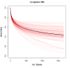
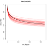
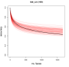
$k_{1}=200$
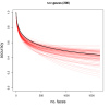
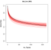
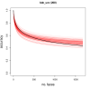
$k_{1}=400$

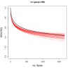
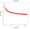
Figure 10: Predicted accuracy curves for face-recognition example: The plots show predicted accuracies. Each red curve represents the predicted accuracies using a single subsample of size $k_{1}$. The black curve shows the average test accuracy obtained from the full data set.

$k_{1}$	ClassExReg	KDE-BCV	KDE-UCV
100	0.113 (0.002)	0.053 (0.001)	0.082 (0.001)
200	0.058 (0.002)	0.037 (0.001)	0.057 (0.001)
400	0.050 (0.001)	0.024 (0.001)	0.035 (0.001)

Table 2: Face-recognition extrapolation RMSEs: RMSE (se) on predicting $\text{TA}_{1672}$ from $k_{1}$ classes

The results for Telugu OCR classification are displayed in Table 3. If we rank the three extrapolation methods in terms of distance to the ground truth accuracy, we see a consistent pattern of rankings between the 20-to-100 extrapolation and the 100-to-400 extrapolation. As we remarked in the simulation, the difficulty of extrapolation appears to be primarily sensitive to the extrapolation ratio $\frac{k_{2}}{k_{1}}$, which are similar (5 versus 4) in the 20-to-100 and 100-to-400 problems. In both settings, ClassExReg comes closest to the ground truth for the Deep CNN and the SVM, but KDE-BCV comes closest to ground truth for the Logistic regression. However, even for logistic regression, ClassExReg does better or comparably to KDE-UCV.

In the 20-to-400 extrapolation, which has the highest extrapolation ratio ($\frac{k_{2}}{k_{1}}=20$), none of the three extrapolation methods performs consistently well for all three classifiers. It could be the case that the variability is a dominating effect given the small training set, making it difficult to compare extrapolation methods using the 20-to-400 extrapolation task.

Unlike in the face recognition example, we did not resample training classes here, because that would require retraining all of the classifiers–which would be prohibitively time-consuming for the Deep CNN. Thus, we cannot comment on the robustness of the comparisons from this example, though it is likely that we would obtain different rankings under a new resampling of the training classes.

$k_{1}$	$k_{2}$	Classifier	True	ClassExReg	KDE-BCV	KDE-UCV
20	100	Deep CNN	0.9908	0.9905	0.7138	0.6507
		Logistic	0.8490	0.8980	0.8414	0.8161
		SVM	0.7582	0.8192	0.6544	0.5771
20	400	Deep CNN	0.9860	0.9614	0.4903	0.3863
		Logistic	0.7107	0.8824	0.7467	0.7015
		SVM	0.5452	0.6725	0.5163	0.4070
100	400	Deep CNN	0.9860	0.9837	0.8910	0.8625
		Logistic	0.7107	0.7214	0.7089	0.6776
		SVM	0.5452	0.5969	0.4369	0.3528

Table 3: Telugu OCR extrapolated accuracies: Extrapolating from $k_{1}$ to $k_{2}$ classes in Telugu OCR for three different classifiers: logistic regression, support vector machine, and deep convolutional network

6 Discussion

In this work, we suggest treating the class set in a classification task as random, in order to extrapolate classification performance on a small task to the expected performance on a larger unobserved task. We show that average generalized accuracy decreases with increased label set size like the $(k-1)$th moment of a distribution function. Furthermore, we introduce an algorithm for estimating this underlying distribution, that allows efficient computation of higher order moments. Code for the methods and the simulations can be found in https://github.com/snarles/ClassEx.

There are many choices and simplifying assumptions used in the description of the method. In this discussion, we discuss these decisions and map some alternative models or strategies for future work.

Since our analysis is currently restricted to i.i.d. sampling of classes, one direction for future work is to generalize the sampling mechanism, such as to cluster sampling. More broadly, the assumption that the labels in $\mathcal{S}_{k}$ are a random sample from a homogeneous distribution $\pi$ may be inappropriate. Many natural classification problems arise from hierarchically partitioning a space of instances into a set of labels. Therefore, rather than modeling $\mathcal{S}_{k}$ as a random sample, it may be more suitable to model it as a random hierarchical partition of $\mathcal{Y}$, such as one arising from an optional Pólya tree process (Wong and Ma, 2010). Finally, note that we assume no knowledge about the new class-set except for its size. Better accuracy might be achieved if some partial information is known.

Also, we only discussed extrapolating the classification accuracy–or equivalently, the risk for the zero-one cost function. However, it is possible to extend our analysis to risk functions with arbitrary cost functions, which is the subject of forthcoming work.

A third direction of exploration is impose additional modeling assumptions for specific problems. ClassExReg adopts a non-parametric model of the discriminability function $D(u)$, in the sense that $D(u)$ was defined via a spline expansion. However, an alternative approach is to assume a parametric family for $D(u)$ defined by a small number of parameters. In forthcoming work, we show that under certain limiting conditions, $D(u)$ is well-described by a two-parameter family. This substantially increases the efficiency of estimation in cases where the limiting conditions are well-approximated.

References

- Abramovich and Pensky (2015) F. Abramovich and M. Pensky. Feature selection and classification of high-dimensional normal vectors with possibly large number of classes. arXiv preprint arXiv:1506.01567, 2015.
- Achanta and Hastie (2015) R. Achanta and T. Hastie. Telugu OCR framework using deep learning. arXiv preprint arXiv:1509.05962, 2015.
- Amos et al. (2016) B. Amos, B. Ludwiczuk, and M. Satyanarayanan. Openface: A general-purpose face recognition library with mobile applications. Technical report, CMU-CS-16-118, CMU School of Computer Science, 2016.
- Cao et al. (1994) R. Cao, A. Cuevas, and W. G. Manteiga. A comparative study of several smoothing methods in density estimation. Computational Statistics & Data Analysis, 17(2):153–176, 1994.
- Crammer and Singer (2001) K. Crammer and Y. Singer. On the algorithmic implementation of multiclass kernel-based vector machines. Journal of Machine Learning Research, 2(Dec):265–292, 2001.
- Davis et al. (2011) J. Davis, M. Pensky, and W. Crampton. Bayesian feature selection for classification with possibly large number of classes. Journal of Statistical Planning and Inference, 141(9):3256–3266, 2011.
- Deng et al. (2010) J. Deng, A. C. Berg, K. Li, and L. Fei-Fei. What does classifying more than 10,000 image categories tell us? In European conference on computer vision, pages 71–84. Springer, 2010.
- Donahue et al. (2014) J. Donahue, Y. Jia, O. Vinyals, J. Hoffman, N. Zhang, E. Tzeng, and T. Darrell. Decaf: A deep convolutional activation feature for generic visual recognition. In International conference on machine learning, pages 647–655, 2014.
- Duygulu et al. (2002) P. Duygulu, K. Barnard, J. F. de Freitas, and D. A. Forsyth. Object recognition as machine translation: Learning a lexicon for a fixed image vocabulary. In European conference on computer vision, pages 97–112. Springer, 2002.
- Griffin et al. (2007) G. Griffin, A. Holub, and P. Perona. Caltech-256 object category dataset. 2007.
- Gupta et al. (2014) M. R. Gupta, S. Bengio, and J. Weston. Training highly multiclass classifiers. Journal of Machine Learning Research, 15(1):1461–1492, 2014.
- Huang et al. (2007) G. B. Huang, M. Ramesh, T. Berg, and E. Learned-Miller. Labeled faces in the wild: A database for studying face recognition in unconstrained environments. Technical Report 07-49, University of Massachusetts, Amherst, October 2007.
- Kay et al. (2008) K. N. Kay, T. Naselaris, R. J. Prenger, and J. L. Gallant. Identifying natural images from human brain activity. Nature, 452(March):352–355, 2008.
- Lee et al. (2004) Y. Lee, Y. Lin, and G. Wahba. Multicategory support vector machines: Theory and application to the classification of microarray data and satellite radiance data. Journal of the American Statistical Association, 99(465):67–81, 2004.
- Oquab et al. (2014) M. Oquab, L. Bottou, I. Laptev, and J. Sivic. Learning and transferring mid-level image representations using convolutional neural networks. In Proceedings of the IEEE conference on computer vision and pattern recognition, pages 1717–1724, 2014.
- Pan et al. (2016) R. Pan, H. Wang, and R. Li. Ultrahigh-dimensional multiclass linear discriminant analysis by pairwise sure independence screening. Journal of the American Statistical Association, 111(513):169–179, 2016.
- Pan and Yang (2010) S. J. Pan and Q. Yang. A survey on transfer learning. IEEE Transactions on knowledge and data engineering, 22(10):1345–1359, 2010.
- Scott (1992) D. W. Scott. Multivariate Density Estimation: Theory, Practice, and Visualization. Wiley, 1992.
- Shannon (1948) C. E. Shannon. A Mathematical Theory of Communication. Bell System Technical Journal, 27(3):379–423, 1948.
- Sharif Razavian et al. (2014) A. Sharif Razavian, H. Azizpour, J. Sullivan, and S. Carlsson. CNN features off-the-shelf: an astounding baseline for recognition. In Proceedings of the IEEE conference on computer vision and pattern recognition workshops, pages 806–813, 2014.
- Stamatatos et al. (2014) E. Stamatatos, W. Daelemans, B. Verhoeven, P. Juola, A. López-López, M. Potthast, and B. Stein. Overview of the author identification task at PAN 2014. In CLEF (Working Notes), pages 877–897, 2014.
- Togneri and Pullella (2011) R. Togneri and D. Pullella. An overview of speaker identification: Accuracy and robustness issues. IEEE Circuits and Systems Magazine, 11(2):23–61, 2011.
- Weston and Watkins (1999) J. Weston and C. Watkins. Support vector machines for multi-class pattern recognition. In ESANN, volume 99, pages 219–224, 1999.
- Wong and Ma (2010) W. H. Wong and L. Ma. Optional Pólya tree and Bayesian inference. The Annals of Statistics, 38(3):1433–1459, 2010.