Tensor network complexity of multilinear maps

Abstract.

We study tensor networks as a model of arithmetic computation for evaluating multilinear maps. These capture any algorithm based on low border rank tensor decompositions, such as $O(n^{\omega+\epsilon})$ time matrix multiplication, and in addition many other algorithms such as $O(n\log n)$ time discrete Fourier transform and $O^{*}(2^{n})$ time for computing the permanent of a matrix. However tensor networks sometimes yield faster algorithms than those that follow from low-rank decompositions. For instance the fastest known $O(n^{(\omega+\epsilon)t})$ time algorithms for counting $3t$-cliques can be implemented with tensor networks, even though the underlying tensor has border rank $n^{3t}$ for all $t\geq 2$. For counting homomorphisms of a general pattern graph $P$ into a host graph on $n$ vertices we obtain an upper bound of $O(n^{(\omega+\epsilon)\operatorname{bw}(P)/2})$ where $\operatorname{bw}(P)$ is the branchwidth of $P$. This essentially matches the bound for counting cliques, and yields small improvements over previous algorithms for many choices of $P$.

While powerful, the model still has limitations, and we are able to show a number of unconditional lower bounds for various multilinear maps, including:

1. an $\Omega(n^{\operatorname{bw}(P)})$ time lower bound for counting homomorphisms from $P$ to an $n$-vertex graph, matching the upper bound if $\omega=2$. In particular for $P$ a $v$-clique this yields an $\Omega(n^{\lceil 2v/3\rceil})$ time lower bound for counting $v$-cliques, and for $P$ a $k$-uniform $v$-hyperclique we obtain an $\Omega(n^{v})$ time lower bound for $k\geq 3$, ruling out tensor networks as an approach to obtaining non-trivial algorithms for hyperclique counting and the Max-$3$-CSP problem.

2. an $\Omega(2^{0.918n})$ time lower bound for the permanent of an $n\times n$ matrix.

1. Introduction

One of the cornerstones of the theory of computation is the study of efficient algorithms:

For a function $f$, how much time is required to evaluate $f$ on given inputs?

Answering this question for almost any specific $f$ is well beyond reach of contemporary tools. For example, it is theoretically possible that canonical NP-complete problems, such as the Circuit Satisfiability problem, can be solved in linear time whereas they are widely believed to require super-polynomial (or somewhat less widely, exponential) time [45, 49, 50]. The main reason for this barrier to quantitative understanding is that it is very hard to prove lower bounds for explicit functions in general models of computation such as circuits or Turing machines.

This situation withstanding, a more modest program to advance our understanding of computation is to study restricted models of computation that for many $f$ of interest are simultaneously

1. general enough to capture the fastest-known algorithms for $f$, and

2. restricted enough to admit proofs of strong unconditional time lower bounds for $f$.

There is a substantial body of existing work that fits under this program, ranging from the study of low-depth or otherwise restricted circuits (see e.g. [7], Ch. 14) to models of algorithm-design principles such as greedy algorithms, backtracking, or dynamic programming [3, 38], to linear or semidefinite programming relaxations for hard combinatorial optimization problems [68].

1.1. Multilinear maps

One class of functions $f$ that are of substantial importance is the family of $\ell$-linear maps (multilinear maps) from $\ell$ input vector spaces to an output vector space. Examples range from maps of known near-linear-time complexity in the input size, such as the discrete Fourier transform [33, 94], to maps without known polynomial-time-complexity algorithms, such as the permanent of a matrix [86, 92]. Beyond motivation in numerical multilinear algebra and its applications, recent advances in the study of fine-grained algorithm design and complexity have highlighted the fundamental role of algebraic methods in the fastest-known algorithm designs across a broad range of tasks from graph problems, such as all-pairs shortest paths and $k$-clique, to parsing and constraint satisfaction problems, such as maximum satisfiability and graph coloring [2, 15, 17, 41, 51, 72, 98, 99].

In this paper, we study the arithmetic complexity of evaluating a multilinear map, that is, the number of operations (scalar additions, subtractions, and multiplications) needed to evaluate the map. To set up a baseline, a generic $\ell$-linear map from $\ell$ vector spaces of dimension $n$ to a scalar requires $\Omega(n^{\ell})$ scalars to represent the map directly using combinations of basis vectors. Given this complexity of a direct explicit representation, it is a fundamental problem to seek less costly representations, along with associated efficient algorithms that work on the chosen representation.

We propose the systematic study of tensor networks on hypergraphs as a framework for fast evaluation of multilinear maps, and show a number of upper and lower bounds on the computational power of tensor networks in the spirit of (i) and (ii) above.

1.2. Tensor networks

Tensor networks have a long and rich history which can be traced as far back as 19-century studies in invariant theory due to Cayley [25, 26], Clebsch [29], Clifford [30], Sylvester [91], and Kempe [54, 55]. Tensor networks are extensively deployed in applications from pure mathematics and theoretical physics [53, 61, 63, 64, 77, 78, 82, 87] to computational physics and chemistry [75, 80, 89]. In theoretical computer science, they appear in various guises including, for example, in the Holant framework [93, 23, 22], in the study of probabilistic graphical models [59, 84], in the study of parallel programming [88], in the study of quantum computing [6], and in the study of arithmetic complexity [9, 24, 37]. Tensor contraction is also emerging as a basic computational primitive in computer hardware [42, 70]. (See Section 1.5 for a detailed discussion.) As the precise definitions are somewhat technical, let us start with a few simple motivating examples and then state our results, with the understanding that precise definitions appear in Section 4.

In our setting, a tensor network is a hypergraph in which the vertices are tensors and the hyperedges are called modes. Each mode that is incident to a tensor defines a “dimension” for indexing the entries of the tensor—for example, a matrix is a tensor that is incident to two modes, one mode for the rows of the matrix, and the other mode for the columns of the matrix. A network may be simplified by a sequence of contractions, where each contraction takes a subset of tensors and replaces it with a single tensor whose entries are obtained as generalized inner products of the entries of the tensors being contracted.

As a concrete first example of these concepts, let us consider the task of multiplying two matrices, $A$ and $B$. More specifically, let $A$ be a matrix with rows indexed by mode $i$ and columns indexed by mode $k$, and let $B$ be a matrix with rows indexed by mode $k$ and columns indexed by mode $j$. We may represent the multiplication task as the tensor network depicted on the left in (1). The result of contracting $A$ and $B$ is a new matrix with rows indexed by $i$ and columns indexed by $j$, where the entry at each position $(i,j)$ is $\sum_{k}A_{ik}B_{kj}$. If the three index sets all have size $n$, then computing $A\cdot B$ by contracting them in such a direct manner uses $\Theta(n^{3})$ operations. To obtain faster matrix multiplication, we can rewrite the bare-bones network on the left in (1) using a low-rank decomposition of the matrix multiplication tensor. For example, Strassen’s decomposition [90] of $2\times 2$ matrix multiplication can be represented using the second network in (1). Note that the index $i$ used by $A$ and the result has been separated into two distinct indices $i$ and $i^{\prime}$, and similarly for $j$ and $k$.

(1)

We can execute the network by succesively contracting groups of vertices. In (2) we see the process of successively contracting pairs of tensors in a carefully chosen order, until only a single tensor – the result of the computation – remains. Such an execution can be naturally represented by a rooted binary tree, as shown on the right in (2), where the tensors of the network form the leaves, and each internal node represents the result of contracting its two children. To summarize, a tensor-network algorithm is specified by providing (a) a tensor network that when contracted yields the desired result, and (b) an execution tree indicating the order in which to contract tensors in the network.

(2)

The cost of performing one of the contractions in an execution is the product of the lengths of the modes used by any tensor involved in the contraction. This simply measures (up to a constant factor) the number of arithmetic operations (additions/multiplications) used to compute the result by a direct, naïve computation that does not depend on the values of the tensors. For example, the contraction of $\alpha$ and $A$ in the first step of (2) has cost $28$ because it involves the three modes $i^{\prime}$ (length $2$), $k$ (length $2$) and $\ell$ (length $7$).

We observe that cost is data-oblivious – the tensor $\alpha$ is fixed with many zero-entries but these entries still contribute to the cost. Indeed, in many cases there may be faster ways of evaluating a contraction than to evaluate it naively, and just like we saw above, this can often be dealt with by rewriting the network appropriately. For instance, consider now the multiplication of two $2^{k}\times 2^{k}$ matrices. Because the family of matrix multiplication tensors is closed under Kronecker products, this operation may be computed by a tensor network like the one shown in (3) (depicting the case $k=5$), where $\alpha$, $\beta$ and $\gamma$ are as in (2). The rows/columns of the matrices are now indexed by $k$-tuples of bits. The execution of this network contracts one $\alpha$/$\beta$/$\gamma$ tensor at a time, which lets us keep the cost low. For example, the first contraction of $A$ with the first $\alpha$ block has a cost of $2^{k}\cdot 2^{k}\cdot 7$, and results in a tensor of size $2^{k-1}\times 2^{k-1}\times 7$, then the next contraction has a cost of $2^{k-1}\cdot 2^{k-1}\cdot 7^{2}$ and produces a result of size $2^{k-2}\times 2^{k-2}\times 7\times 7$, and so on, until the contraction with the last $\alpha$ block which has a cost of $2\cdot 2\cdot 7^{k}=O(7^{k})$, and all the contractions in the execution have cost bounded by this, meaning that we get a total running time of $O(k7^{k})=O(N^{\log_{2}7}\log N)$ for $N\times N$ matrices.

(3)

This type of argument can capture any algorithm based on a low-rank decomposition of the underlying tensor of the multilinear map, and indeed, this enables $O(n^{\omega})$-time matrix multiplication using tensor networks. Beyond simple low-rank decompositions, which always give rise to “star-like” networks as in (3), there are many interesting algorithms that can be captured using networks with a more complicated topology. For instance, many maps of substantial importance have a layered structure that decomposes the map to a sequence of elementary maps. A canonical example is the discrete Fourier transform (DFT), which for a smooth composite order such as $2^{k}$, can be decomposed into a fast Fourier transform (FFT) that consists of a sequence of $k$ transforms of order $2$ interleaved with diagonal-matrix multiplications of twiddle factors [33, 94].

1.3. Our results

Starting with motivation (i) and seeking to express existing fastest-known algorithms as executions of tensor networks by a sequence of contractions, we show upper bounds for a number of natural problems. Beyond standard linear settings such as the FFT, not only do tensor networks realize classical bilinear settings such as Abelian group algebra products and fast matrix multiplication algorithms based on low tensor rank, they are powerful enough to capture a substantial number of higher-linearity applications, including Ryser’s algorithm for matrix permanent [86], and the Kruskal operator [57, 60] (cf. Section 3.5), which underlies realization of rank-decompositions for tensor rank [58] and current fastest algorithms for detecting outlier correlations [52].

One problem for which tensor networks turn out to be particularly useful is counting homomorphisms from a fixed pattern graph $P$ to a large host graph $G$ on $n$ vertices. The most well-studied such problem is when $P$ is a $k$-clique. For this problem, the currently fastest algorithm runs in time roughly $O(n^{\omega k/3})$ (with variations in the exponent depending on $k\bmod 3$) [72, 41]. For general $P$, it is known that the problem can be solved in $O(n^{\operatorname{tw}(P)+1})$ time [39], where $\operatorname{tw}(P)$ is the treewidth of $P$. We show that tensor networks can solve the problem in $O(n^{(\omega+\epsilon)\operatorname{bw}(P)/2})$ time, where $\operatorname{bw}(P)$ is the branchwidth of $P$. For $P$ a $k$-clique we have $\operatorname{bw}(P)=\lceil 2k/3\rceil$ so this almost recovers the $O(n^{\omega k/3})$ running time, and in this case we can slightly improve the running time to recover the $O(n^{\omega\lfloor k/3\rfloor+(k\bmod 3)})$ time of Nešetřil and Poljak [72]. In the case of general $P$, this improves on the treewidth-based bound for graphs with $\operatorname{bw}(P)\leq 2(\operatorname{tw}(P)+1)/\omega$ (and in particular if $\omega=2$ it is always as fast as the treewidth-based bound, ignoring the $\epsilon$). By recent results of Curticapean, Dell, and Marx [34], fast algorithms for homomorphism-counting can be used to obtain fast algorithms for counting subgraphs of $G$ isomorphic to $P$, and in some cases our new branchwidth-based bound leads to an improvement; for example, for counting paths of lengths of length $7$, $8$ or $9$, we get a running time of $O(n^{3\omega/2+\epsilon})<O(n^{3.56})$ compared to $O(n^{4})$ using the treewidth-based bound, whereas for very long paths it is not clear whether we would need $\omega=2$ in order for these bound to improve on the treewidth-based bound. Previous work that combines branch decompositions and fast matrix multiplication includes Dorn [40] and Bodlaender et al. [19].

Further applications captured by tensor networks are the set covering and set partitioning frameworks via fast zeta and Möbius transforms that underlie the current fastest algorithms for graph coloring [17] and its generalizations such as computing the Tutte polynomial [14, 15]. To summarize, we have the following compendium theorem of upper bound results. For the detailed definitions of the relevant multilinear maps, cf. Section 3 and Section 5.

Theorem 1.1.

We have the following upper bounds on arithmetic complexity via tensor networks:

1. $O(n^{\omega+\epsilon})$ for the matrix multiplication map of two $n\times n$ matrices.

2. $O(n^{(\omega+\epsilon)\lfloor v/3\rfloor+(v\bmod 3)})$ for counting $v$-cliques in an $n$-vertex graph.

3. $O(n^{(\omega+\epsilon)\operatorname{bw}(P)/2})$ for counting homomorphisms of a fixed pattern (hyper)graph $P$ into a (hyper)graph on $n$ vertices.

4. $O(\max(n^{\lceil\ell/2\rceil(\omega+\epsilon-1)}r,\,n^{2\lceil\ell/2\rceil}r^{\omega+\epsilon-2}))$ for the Kruskal operator of $\ell$ matrices of shape $n\times r$.

5. $O(2^{k}k)$ for the discrete Fourier transforms for the Abelian groups $\mathbb{Z}_{2^{k}}$ and $\mathbb{Z}_{2}^{k}$.

6. $O(2^{k}k)$ for group algebra products on $\mathbb{F}[\mathbb{Z}_{2^{k}}]$ and $\mathbb{F}[\mathbb{Z}_{2}^{k}]$ when $2$ is unit in $\mathbb{F}$.

7. $O(2^{k}k)$ for the semigroup algebra product on $\mathbb{F}[(\{0,1\}^{k},\subseteq,\cap,\cup)]$.

8. $O(2^{n}n)$ for the permanent of an $n\times n$ matrix.

Above $\epsilon>0$ is an arbitrary constant.

Perhaps the most interesting application above is the $v$-clique problem, which suggests that one should seek to pursue generalizations to $v$-vertex hypercliques of $\binom{v}{k}$ hyperedges with $v>k\geq 3$. Indeed, subgraph counting is a problem that has received substantial interest over the years (e.g. [51, 72, 5, 4, 41, 16, 18, 100, 96, 44, 43, 74, 56, 34]), but progress in the particular case of $v$-clique has been stuck to the extent that the problem has attracted notoriety as a hardness assumption in fine-grained complexity [1, 2]. Beyond the study of cliques, hypercliques, and subgraph counting, nontrivial algorithms for such forms would have immediate applicability, for example, in the study of maximum constraint satisfaction problems (Max-CSP) for constraints of width $k\geq 3$; cf. Williams [98] for the case $k=2$. One of the main goals of our subsequent lower bounds is to rule out tensor networks as a candidate to yield improved algorithms in this setting.

Turning from upper bounds to lower bounds and motivation (ii), tensor networks are restricted enough to enable nontrivial lower bounds for many multilinear maps. To begin with, an immediate limitation of tensor networks is that all the intermediate results during the execution of a network are multilinear, and the execution of a network can be simulated by a multilinear circuit. Raz [81] shows that multilinear formulas cannot compute the determinant of an $n\times n$ matrix in a polynomial number of operations in $n$, even though polynomial-size general circuits are known for the determinant (cf. [11, 20, 85]).

It turns out that considerably stronger lower bounds can be shown for tensor networks. In particular, we establish essentially tight lower bounds (subject to the assumption $\omega=2$) for arithmetic complexity via tensor networks of $P$-homomorphism counting and the Kruskal operator. Furthermore, we rule out the possibility of any nontrivial algorithm designs via tensor networks for counting cliques in hypergraphs. The following theorem collects our main lower-bound results, and should be contrasted with the upper bounds in Theorem 1.1.

Theorem 1.2.

We have the following lower bounds on arithmetic complexity via tensor networks:

1. $\Omega(n^{\operatorname{bw}(P)})$ for the multilinear form corresponding to $P$-homomorphism counting. In particular, this yields a lower bound of $\Omega(n^{\lceil 2v/3\rceil})$ for counting cliques of size $v$, and a lower bound of $\Omega(n^{v})$ for counting hypercliques of size $v$.

2. $\Omega(\max(n^{\ell},n^{\lceil l/2\rceil}r))$ for the Kruskal operator of $\ell$ matrices of shape $n\times r$.

3. $\Omega(\binom{n}{n/3})$ for the determinant or permanent of an $n\times n$ matrix.

We remark that [69] independently showed that the border rank of the $v$-hyperclique tensor is $\Omega(n^{v})$; our $\Omega(n^{v})$ lower bound for tensor networks strengthens that. One may wonder about the gap between the bounds of $\Omega(\binom{n}{n/3})$ and $O(2^{n}n)$ for the permanent. As we explain below, our lower bound methods are inherently rank-based and cannot go beyond $\binom{n}{n/3}$. A curious point is that it is not immediately clear whether tensor networks can even achieve $O^{*}(2^{n})$ time for the determinant, and we do not know whether or not this is possible.

1.4. Overview of proof ideas

As a running example in this overview, we consider the $6$-linear forms $A:\mathbb{F}^{[n]\times[n]}\times\mathbb{F}^{[n]\times[n]}\times\ldots\times\mathbb{F}^{[n]\times[n]}\rightarrow\mathbb{F}$ taking as input $6$ matrices of size $n\times n$, defined by

$$A(X^{(1)},X^{(2)},X^{(3)},X^{(4)},X^{(5)},X^{(6)})=\sum_{i,j,k,\ell\in[n]}X^{(1)}_{ij}X^{(2)}_{ik}X^{(3)}_{i\ell}X^{(4)}_{jk}X^{(5)}_{j\ell}X^{(6)}_{k\ell}\,.$$ (4)

If $\chi$ is the adjacency matrix of a loopless graph $G$, then $A(\chi,\chi,\chi,\chi,\chi,\chi)$ counts the number of $4$-cliques in the graph. Associated with $A$ is the $6$-tensor $T(A)$ of size $n^{2}\times n^{2}\times\cdots\times n^{2}$, where each of the $6$ modes is indexed by a pair $(i,j)\in[n]\times[n]$, and the value at a given position is the coefficient of the corresponding term in $A$. Concretely,

$$T(\!A)_{i_{1}j_{1},i_{2}k_{2},i_{3}\ell_{3},j_{4}k_{4},j_{5}\ell_{5},k_{6}\ell_{6}}\!=\!\!\begin{cases}1&\!\!\!\text{if $i_{1}=i_{2}=i_{3}$, $j_{1}=j_{4}=j_{5}$, $k_{2}=k_{4}=k_{6}$ $\wedge$ $\ell_{3}=\ell_{5}=\ell_{6}$},\\ 0&\!\!\!\text{otherwise}.\end{cases}$$

Upper bounds

Most, but not all, of the families of multilinear maps we consider are closed under taking Kronecker products. For instance, consider the $4$-clique counting form (4) for an $n$-vertex graph and its associated tensor $T(A)$. Then for any $k\geq 1$, the tensor associated with the $4$-clique counting form in $n^{k}$-vertex graphs is $T(A)^{\otimes k}$, the $k$-fold Kronecker product of $T(A)$ with itself. We write $A^{\otimes k}$ for the associated map. With this in mind, it is natural to seek general constructions that, given an efficient evaluation of some map $A$, yields an efficient evaluation of $A^{\otimes k}$.

We give such a construction, and show that the cost of the best tensor network execution for $A^{\otimes k}$ is essentially submultiplicative in a quantity that we call the amortized cost of an execution. For tensors of order at most $3$, the notion of amortized cost essentially captures the rank of $T(A)$, but for higher-order tensors, the amortized cost may be significantly smaller than the rank. Roughly speaking, the amortized cost of a step in an execution of a map $A$ is: (i) equal to the normal cost if the operation involves the contraction of two tensors that both depend on some input variables of $A$, but (ii) equal to the size of the result if only one of the tensors involved in the contraction depends on the input variables of $A$. A precise definition appears in Section 5.1. Our general upper bound for the cost of $A^{\otimes k}$ can, somewhat informally, be stated as follows.

Theorem 1.3 (Submultiplicativity of cost, informal statement).

If a multilinear map $A$ has a tensor network execution consisting of $s$ steps, each with cost at most $c$ and amortized cost at most $a$, then $A^{\otimes k}$ has a tensor network execution consisting of at most $k\cdot s$ steps, each with cost at most $a^{k-1}\cdot c$.

An immediate corollary of this is that we can capture any algorithm for $A^{\otimes k}$ based on a low-rank decomposition of $T(A)$ (5.2). For example, this implies that tensor networks can multiply $n\times n$ matrices in $O(n^{\omega+\epsilon})$ time (Section 5.2).

However, returning to our running example form (4), as we explain below the tensor $T(A)$ has rank $n^{4}$, meaning that 5.2 only yields a trivial upper bound. This is where the full generality of 1.3 comes in. Consider the form (4) for graphs on some constant number $n_{0}$ of vertices. As it turns out, we can design a network and an associated execution for this form, depicted in (5) and explained in more detail in the proof of 5.11, with an execution of cost $n_{0}^{2e+3}$ and amortized cost $n_{0}^{e+1}$, where $n_{0}^{e}$ is the rank of the tensor associated with $n_{0}\times n_{0}$ matrix multiplication. Picking $n_{0}$ to be a large enough constant so that $e$ is approximately $\omega$, and letting $k$ be such that $n$ is approximately $n_{0}^{k}$, we obtain via 1.3 an $O(n^{\omega+\epsilon+1})$ time upper bound for (4).

(5)

Lower bounds

Just like many other arithmetic complexity lower bounds, our lower bounds boil down to establishing lower bounds on the rank of certain matrices.

In order to establish a lower bound on the rank of $T(A)$, we flatten it to a matrix and analyze the rank of that matrix. There are $2^{5}$ possible bipartitions of the $6$ modes of $T(A)$ into two non-empty subsets, and the lower bound on the rank of $T(A)$ that we obtain is the maximum of the ranks of the resulting matrices. Using this method it is easy to establish that for our example form (4), the rank of $T(A)=n^{4}$. That this is an upper bound follows from (4), and that it is a lower bound follows by considering the bipartition taking variables $X^{(1)}$ and $X^{(6)}$ as row indices, and the other $4$ variables as column indices. The resulting $n^{4}\times n^{8}$ matrix has full rank.

Tensor networks are more versatile and can be more efficient than low-rank decompositions of $T(A)$. Nevertheless, we show limitations on this versatility. In particular we show that every tensor network execution for $A$ induces a tree in which the leaves are the inputs of $A$ and all internal vertices have degree $3$. We call this a socket tree. Each edge in a socket tree induces a bipartition of the variables and our key technical lemma is to show that for each such bipartition, the rank of the corresponding flattening of $T(A)$ is a lower bound on the cost of the execution that gave rise to the tree. Thus, to obtain a lower bound for the cost of a specific execution, we consider the maximum rank obtained over all edges of the corresponding socket tree, and to lower bound the cost of every tensor network execution, we minimize this quantity over all possible socket trees. We refer to the resulting quantity as the socket width of $A$, denoted $w(A)$ (formal definition appears in Section 6). Our general lower bound can thus be phrased as follows, where $c(A)$ denotes the minimum cost of a tensor network for evaluating $A$ (formal definition appears in Section 4.5).

Theorem 1.4.

For every multilinear map $A$, it holds that $c(A)\geq w(A)$.

Indeed, for our running example (4), there are low-width socket trees establishing that $w(A)\leq n^{3}$, see (6). However, that bound is tight: our $\Omega(n^{\lceil 2\cdot 4/3\rceil})=\Omega(n^{3})$ lower bound for the $\binom{4}{2}$-linear form (1.2) is obtained by proving that $w(A)\geq n^{3}$ (7.4) and appealing to 1.4.

(6)

1.5. Earlier and related work

We now proceed to a more detailed discussion of earlier work.

Tensor networks

The history of tensor networks (or, alternatively, tensor diagrams or diagrams) as an analytical and computational tool goes back to the 19-century to the works by Cayley [25, 26], Clebsch [29], Clifford [30], Sylvester [91], and Kempe [54, 55]. The diagrammatic form used here can be traced back to Penrose [78]. Some early appearances of tensor diagrams are by Cvitanovic̀ [35], Cvitanovic̀ and Kennedy [36], Kuperberg [61], and many others. Surveys of tensor diagrams can be found in Penrose and Rindler [79] and Landsberg [63]. Schrijver [87] gives a brief historical account.

A principal deviation from Penrose’s notation that we make in this paper is to work subject to a basis and a corresponding dual basis in each relevant vector space to avoid distinction between primal and dual spaces. This in particular enables a concise treatment of hyperedges and saves us from considering orientation of edges, or the planar layout of edges in a drawing. That is, we will view a tensor network combinatorially as a hypergraph with tensors associated at the vertices, and with a subset of the hyperedges designated to form the boundary of the network (cf. Section 4 for the precise definitions). A yet further conceptual difference is that we view the execution of a tensor network as a sequence of contractions of sets of vertices (tensors) rather than as contractions of hyperedges (modes). This choice enables us to reduce the size of hyperedges gradually before eliminating them during an execution, thus enabling better granularity. For simplicity, we will restrict to a purely multilinear framework and will not consider sums of networks although such a study would be possible, and is pursued e.g. in Penrose’s work [78].

A large body of existing work in applications (cf. Section 1.2) studies how to efficiently execute a given tensor network $D$. Our quest in this paper differs from such studies in that we study a multilinear map $A$, and seek to design the most efficient network $D$ that realizes $A$, or to establish lower bounds for best-possible designs. In particular, our upper and lower bounds in 1.1 and 1.2 are over all tensor networks that realize a particular map $A$ of interest.

Computational problems on tensors and tensor networks

Problems on given tensors and tensor networks are known to be mostly computationally hard as soon as the setting changes from matrices to higher-order tensors. Håstad [46] showed that computing the rank of an explicitly given $\ell$-tensor is NP-complete over finite fields and NP-hard over rationals whenever $\ell\geq 3$. Hillar and Lim extended the latter result to any field containing $\mathbb{Q}$ [47]. They also showed that many other tensor problems such as the eigenvalue, singular value and spectral norm decision and approximation problems as well as rank-1 approximation problem for 3-tensors (over $\mathbb{R}$ and in some cases over $\mathbb{C}$) are NP-hard.

The task of finding the value of a given scalar-valued tensor network is known to be $\#$P-complete (see e.g. [8, 12]). Similarly, it is NP-hard to find the most efficient sequence of contractions for a given network [62, 80].

Tensor networks in applications

Beyond our present use of tensor networks as a model of computation to efficiently evaluate multilinear maps, tensor networks are used across a broad range of applications. Accordingly, the following should be viewed as mere pointers to further literature on tensor networks, not as an exhaustive listing of all applications of tensor networks. Orus [75] gives an introduction to tensor networks in the context of computational physics. Itai and Landau [6] study quantum computation and quantum algorithms for evaluating tensor networks [6]. Solomonik and Hoefler study sparse tensor algebra as a model for parallel programming [88]. The Holant framework introduced by Valiant [93] and studied further by Cai et al. [23, 22] involves the study of multilinear sum–product expressions that can be viewed as tensor networks. Tensor networks appear naturally in the study of probabilistic graphical models [59, 71, 84, 97], and in the study of various machine-learning problems [27, 28].

Bilinear and multilinear complexity

As was concisely outlined in Section 1.4, for bilinear maps our present work reduces to the study of tensor rank of 3-tensors and an extensive body of work on bilinear complexity, with the arithmetic complexity of the matrix multiplication map as the primary driver. For two starting points to this literature, we refer to the monograph by Bürgisser, Clausen, and Shokrollahi [21] and to the survey by Pan [76]. Our present work can be seen as generalizing this bilinear theory to higher orders of linearity via tensor networks and their executions. The current state of the art for fast matrix multiplication can be found in Le Gall [66, 67], Le Gall and Urrutia [65], Vassilevska Williams [95], Cohn and Umans [32], Cohn, Kleinberg, Szegedy, and Umans [31], Benson and Ballard [10], and Huang, Rice, Matthews, and van de Geijn [48].

1.6. Organization of this paper

Section 2 recalls preliminaries on tensors, multilinear maps, and branchwidth. Section 3 reviews the specific multilinear maps that we study in this work and describes for each map its associated tensor. In Section 4, tensor networks, execution and cost of a tensor network, and cost of a multilinear map are defined. Section 5 presents tensor-network algorithms for the multilinear maps introduced in Section 3. In Section 6, a general lower bound on the cost of evaluating a multilinear map using tensor network is obtained. The lower bound is expressed in terms of the socket-width of a multilinear map. In Section 7, lower bounds on socket-width for concrete multilinear maps studied in Sections 3 and 5 are derived. Finally, Appendix A gives some background results on minimum-cost executions.

2. Preliminaries

Throughout the paper $[n]$ denotes $\{1,2,\ldots,n\}$ and $\mathbb{F}$ denotes an arbitrary fixed field.

2.1. Tensors

This section sets up our notation for tensors and multilinear maps. We work with tensors and multilinear maps relative to fixed bases for the respective vector spaces over $\mathbb{F}$.

Modes, indexing, and positions

We will work with the following convention of positioning individual entries inside a tensor. Let $E$ be a finite set of modes. Associate with each mode $e\in E$ a finite nonempty index set $J(e)$. In this case we say that $E$ is a set of indexed modes. The length of $e$ is $|J(e)|$. A position is an element $j\in\prod_{e\in E}J(e)$. Let us write $J(E)=\prod_{e\in E}J(e)$ for the set of all positions with respect to the indexed modes $E$. In the special case that the set of modes $E$ is empty we define the set of positions $J(E)$ to consist of a single element.

Tensors, matrices, vectors, and scalars

Let $E$ be a set of indexed modes. A tensor with respect to $E$ is a mapping $T:J(E)\rightarrow\mathbb{F}$. Equivalently, we write $T\in\mathbb{F}^{J(E)}$ to indicate that $T$ is a tensor with respect to the indexed modes $E$. We view the set $\mathbb{F}^{J(E)}$ of all tensors over $E$ as a vector space over $\mathbb{F}$ with addition and scalar multiplication of tensors defined entrywise. We say that $|E|$ is the order of the tensor. A tensor of order zero is called a scalar, a tensor of order one is called a vector, and a tensor of order two is called a matrix. The volume of the tensor is $|J(E)|$. The tuple $(|J(e)|:e\in E)$ is the shape of the tensor. It is convenient to use the “$\times$”-symbol to punctuate the shape of a tensor; that is, instead of writing, say $(2,3,4)$ for the shape, we write $2\times 3\times 4$. For a position $j\in J(E)$ and a tensor $T\in\mathbb{F}^{J(E)}$, we say that $T_{j}\in\mathbb{F}$ is the entry of $T$ at $j$.

A flattening of $T$ induced by a bipartition $E_{1}\cup E_{2}=E$ of the modes of $T$ is a $|J(E_{1})|\times|J(E_{2})|$ matrix $M$ where, for $j_{1}\in J(E_{1})$ and $j_{2}\in J(E_{2})$ we have $M_{j_{1},j_{2}}=T_{j_{1}j_{2}}$. Given two order $\ell$ tensors $S\in\mathbb{F}^{[n_{1}]\times[n_{2}]\times\cdots\times[n_{\ell}]}$ and $T\in\mathbb{F}^{[m_{1}]\times[m_{2}]\times\cdots\times[m_{\ell}]}$, their Kronecker product $S\otimes T$ is a tensor in $\mathbb{F}^{[n_{1}m_{1}]\times[n_{2}m_{2}]\times\cdots\times[n_{\ell}m_{\ell}]}$ defined by

$$(S\otimes T)_{m_{1}(i_{1}-1)+j_{1},m_{2}(i_{2}-1)+j_{2},\ldots,m_{\ell}(i_{\ell}-1)+j_{\ell}}=S_{i_{1},i_{2},\ldots,i_{\ell}}T_{j_{1},j_{2},\ldots,j_{\ell}}.$$

2.2. Multilinear maps

Let $E_{1},E_{2},\ldots,E_{\ell},E^{\prime}$ be pairwise disjoint sets of indexed modes such that $E_{1},E_{2},\ldots,E_{\ell}$ are nonempty. We say that a map $A:\mathbb{F}^{J(E_{1})}\times\mathbb{F}^{J(E_{2})}\times\cdots\times\mathbb{F}^{J(E_{\ell})}\rightarrow\mathbb{F}^{J(E^{\prime})}$ is an $\ell$-linear map if $A$ is linear with respect to each of its $\ell$ inputs individually when the other inputs remain fixed. In particular, a $1$-linear map is a linear map. A multilinear map that gives a scalar output is a multilinear form. In particular, $A$ is a form if and only if $E^{\prime}$ is empty.

The tensors of a multilinear map

For an $\ell$-linear map $A:\mathbb{F}^{J(E_{1})}\times\mathbb{F}^{J(E_{2})}\times\cdots\times\mathbb{F}^{J(E_{\ell})}\rightarrow\mathbb{F}^{J(E^{\prime})}\,,$ we define two slightly different tensors $T(A)$ and $\hat{T}(A)$. Both are indexed by $J(E_{1}\cup E_{2}\cup\ldots\cup E_{\ell}\cup E^{\prime})$ and at position $j_{1}j_{2}\ldots j_{\ell}j^{\prime}$ take the value

$$T(A)_{j_{1}j_{2}\ldots j_{\ell}j^{\prime}}=\hat{T}(A)_{j_{1}j_{2}\ldots j_{\ell}j^{\prime}}=A\bigl{(}e^{(j_{1})},e^{(j_{2})},\ldots,e^{(j_{\ell})}\bigr{)}_{j^{\prime}}\,,$$

where $e^{(j_{i})}\in\mathbb{F}^{J(E_{i})}$ denotes the tensor with a $1$ in position $j_{i}$ and $0$s in all other position. The difference between $T(A)$ and $\hat{T}(A)$ is their shape. The shape of $T(A)$ is $|J(E_{1})|\times|J(E_{2})|\times\cdots\times|J(E_{\ell})|\times|J(E^{\prime})|$, except if $A$ is a form in which case the $|J(E^{\prime})|$ part is omitted. Thus $T(A)$ is of order $\ell+1$ (or $\ell$ if $A$ is a form). The shape of $\hat{T}(A)$ is $(|J(e)|:e\in E_{i},i\in[\ell+1])$, thus its order is $|E_{1}|+|E_{2}|+\cdots+|E_{\ell}|+|E^{\prime}|$.

In other words, each mode of $T(A)$ corresponds to one of the inputs of $A$, or the output. These inputs are in turn sets of indexed modes so may contain more “fine-grained” structure, but this information is lost at the level of granularity of $T(A)$. When working with tensor networks for evaluating $A$, we need to keep track of the fine-grained mode structure because this is in many cases what allows us to construct efficient algorithms, hence in most parts of the paper we are more interested in the tensor $\hat{T}(A)$ which contains this fine-grained structure.

On the other hand, $\hat{T}(A)$ does not contain information about which modes are grouped together to form the inputs and output of $A$, and this information is also important. This leads us to the notion of sockets, defined next.

Sockets

Let us study the tensor $\hat{T}(A)$ with respect to the map $A$. We say that the modes in $E_{1}\cup E_{2}\cup\cdots\cup E_{\ell}$ are the input modes of $\hat{T}(A)$, and the modes in $E^{\prime}$ are the output modes of $\hat{T}(A)$ with respect to $A$. Let us say that $E_{1},\ldots,E_{\ell}$ are the input sockets of $\hat{T}(A)$ with respect to $A$. Similarly, $E^{\prime}$ is the output socket in $\hat{T}(A)$ with respect to $A$. In particular, the output socket is empty if and only if $A$ is a form. To describe a socketing of the modes of a tensor, it is convenient to use parentheses to group a “$\times$”-punctuated shape of a tensor into sockets, see also Section 2.1.

Let $\hat{T}$ be a tensor over a set of indexed modes $E$. Any tuple $\mathcal{E}=(E_{1},E_{2},\ldots,E_{\ell},E^{\prime})$ of subsets of $E$ that partitions $E$ with $E_{1},E_{2},\ldots,E_{\ell}$ nonempty defines an $\ell$-linear map $A_{\mathcal{E}}(\hat{T}):\mathbb{F}^{J(E_{1})}\times\mathbb{F}^{J(E_{2})}\times\cdots\times\mathbb{F}^{J(E_{\ell})}\rightarrow\mathbb{F}^{J(E^{\prime})}$ with $\hat{T}(A_{\mathcal{E}}(\hat{T}))=\hat{T}$. In this case the tuple $(E_{1},E_{2},\ldots,E_{\ell})$ gives the input sockets of $T$ and $E^{\prime}$ is the output socket of $\hat{T}$ with respect to $A_{\mathcal{E}}(\hat{T})$.

We thus conclude that two multilinear maps $A_{1},A_{2}$ may have the same base tensor $\hat{T}(A_{1})=\hat{T}(A_{2})$, and from a tensor $\hat{T}$ one may obtain different multilinear maps by varying how the modes of $\hat{T}$ are assigned to input and output sockets.

The form of a multilinear map

Let $A$ be a multilinear map with a nonempty output socket. We can turn $A$ into a multilinear form $F(A)$ by turning its output socket into an input socket. Let us say that $F(A)$ is the multilinear form of $A$. We also set $F(A)=A$ when $A$ is a multilinear form.

2.3. Branch decompositions and branchwidth

A branch decomposition of a (hyper)graph $G$ consists of (i) a tree $T$ whose every vertex has degree either one or three, and (ii) a bijection $\pi$ between the (hyper)edge set of $G$ and the set of vertices of degree one in $T$. Deleting an edge $e\in E(T)$ from $T$ partitions $T$ into two subtrees $T_{1}$ and $T_{2}$ that via $\pi$ give rise to a partition of the (hyper)edges of $G$ into two sets $E_{1}$ and $E_{2}$. The width $w(e)$ of the partition induced by $e$ is the number of vertices of $G$ that are incident to at least one (hyper)edge in $E_{1}$ and at least one (hyper)edge in $E_{2}$. The width of the branch decomposition $(T,\pi)$ is the maximum of the widths $w(e)$ for $e\in E(T)$. The branchwidth $\operatorname{bw}(G)$ of $G$ is the minimum width of a branch decomposition of $G$.

For graphs, we recall the following upper bound on branchwidth.

Claim 2.1 (Robertson and Seymour [83]).

For every $n\geq 3$, $\operatorname{bw}(K_{n})=\lceil 2n/3\rceil$. Consequently, $\operatorname{bw}(G)\leq\lceil 2|V(G)|/3\rceil$ for every graph $G$.

3. Examples of multilinear maps

This section reviews the specific multilinear maps that we study in this work. Together with each map we describe its associated tensor and a socketing of the tensor that realizes the map.

3.1. Discrete Fourier transform

Let $n\geq 2$ be an integer and let $\rho\in\mathbb{F}$ be a primitive $n^{\text{th}}$ root of unity in the field $\mathbb{F}$. Define the $n\times n$ symmetric matrix $\Phi$ with entries $\Phi_{i,j}=\rho^{(i-1)(j-1)}$ for all $i,j\in[n]$. The discrete Fourier transform (DFT) of order $n$ at $\rho$ is the linear map $L:\mathbb{F}^{[n]}\rightarrow\mathbb{F}^{[n]}$ defined for all $x\in\mathbb{F}^{[n]}$ by the matrix-vector multiplication $L(x)=\Phi x$. In particular, the matrix $\Phi$ is the tensor associated with $L$. The matrix $\Phi$ has two modes, namely its rows and columns. To realize $L$, take the columns of $\Phi$ as the input socket, and the rows as the output socket.

3.2. Determinant and permanent

Let us write $S_{n}$ for the symmetric group of all permutations $\sigma:[n]\rightarrow[n]$. Let $c(\sigma)$ be the number of cycles in the cycle decomposition of $\sigma$, where each fixed point of $\sigma$ is counted as a cycle. Further standard examples of multilinear operators include the determinant and permanent

$$\det A =\sum_{\sigma\in S_{n}}(-1)^{n-c(\sigma)}\prod_{i\in[n]}a_{i,\sigma(i)} \operatorname{per}A =\sum_{\sigma\in S_{n}}\prod_{i\in[n]}a_{i,\sigma(i)}\,,$$ (7)

both of which are $n$-linear in the $n$ columns (or the $n$ rows) of the matrix $A=(a_{ij})_{i,j\in[n]}$. The determinant and permanent are associated with order $n$ tensors $\hat{T}^{(\det)},\hat{T}^{(\operatorname{per})}\in\mathbb{F}^{[n]\times[n]\times\cdots\times[n]}$ defined for all $j=(i_{1},i_{2},\ldots,i_{n})\in[n]\times[n]\times\cdots\times[n]$ by

$$\hat{T}^{(\det)}_{j} =\begin{cases}(-1)^{n-c(j)}&\text{if }j\in S_{n}\\ 0&\text{otherwise}\end{cases} \hat{T}^{(\operatorname{per})}_{j} =\begin{cases}1&\text{if }j\in S_{n}\\ 0&\text{otherwise}.\end{cases}$$ (8)

To realize the determinant and permanent using (8), we socket $\hat{T}^{(\det)}$ and $\hat{T}^{(\operatorname{per})}$ with the rows of $A$. The determinant and permanent tensors are not closed under taking Kronecker products, because the Kronecker product of two tensors has the same order as its input tensors, but for each $n$ there is exactly one determinant (permanent) tensor of order $n$.

3.3. Matrix multiplication

Let $n$, $r$, and $m$ be positive integers. Perhaps the most fundamental example of a bilinear map is the map that multiplies an $n\times r$ matrix $A=(A_{ij})_{i\in[n],\,j\in[r]}$ with an $r\times m$ matrix $B=(B_{ij})_{i\in[r],\,j\in[m]}$ to obtain the $n\times m$ product matrix $C=(C_{ij})_{i\in[n]\,,j\in[m]}$ defined for all $i\in[n]$ and $j\in[m]$ by

$$C_{ij}=\sum_{k\in[r]}A_{ik}B_{kj}\,.$$ (9)

It is natural to view the input $A\in\mathbb{F}^{[n]\times[r]}$ as a 2-tensor, and similarly so for the input $B\in\mathbb{F}^{[r]\times[m]}$, and the output $C\in\mathbb{F}^{[n]\times[m]}$. Thus, (9) is naturally associated with the 6-tensor $\hat{T}\in\mathbb{F}^{[n]\times[r]\times[r]\times[m]\times[n]\times[m]}$ with entries defined for all $i_{1},i_{2}\in[n]$, $j_{1},j_{2}\in[m]$, and $k_{1},k_{2}\in[r]$ by

$$\hat{T}_{i_{1}\!k_{1}\!k_{2}j_{1}\!i_{2}j_{2}}=\begin{cases}1&\text{if $i_{1}=i_{2}$ and $j_{1}=j_{2}$ and $k_{1}=k_{2}$};\\ 0&\text{otherwise}.\end{cases}$$ (10)

To realize (9) using (10), we can use the socketing grouped by parentheses in $([n]\times[r])\times([r]\times[m])\times([n]\times[m])$, where the first two groups are the two input sockets corresponding to $A$ and $B$, and the last group is the output socket corresponding to $C$.

Let us write $\langle n,r,m\rangle$ as a shorthand for the tensor (10). From (10) and the definition of the Kronecker product it is immediate that matrix-multiplication tensors satisfy

$$\langle n_{1},r_{1},m_{1}\rangle\otimes\langle n_{2},r_{2},m_{2}\rangle=\langle n_{1}n_{2},r_{1}r_{1},m_{1}m_{2}\rangle\,.$$ (11)

That is, matrix multiplication tensors are closed under taking Kronecker products.

3.4. Group algebra product

Let $(\mathbb{A},+)$ be an Abelian group of order $n$. Another fundamental example of a bilinear map is to convolve two vectors $f\in\mathbb{F}^{\mathbb{A}}$ and $g\in\mathbb{F}^{\mathbb{A}}$ according to the group operation of $\mathbb{A}$ to obtain the vector $h=f*g\in\mathbb{F}^{\mathbb{A}}$, defined for all $k\in\mathbb{A}$ by

$$h_{k}=\sum_{j\in\mathbb{A}}f_{(k-j)}\,g_{j}\,.$$ (12)

The map (12) is associated with the $3$-tensor $\hat{T}\in\mathbb{F}^{\mathbb{A}\times\mathbb{A}\times\mathbb{A}}$ defined for all $i,j,k\in\mathbb{A}$ by

$$\hat{T}_{ijk}=\begin{cases}1&\text{$i+j=k$};\\ 0&\text{otherwise}.\end{cases}$$ (13)

A socketing of the three modes of (13) that realizes (12) is to take the first two modes as two input sockets corresponding to $f$ and $g$, respectively, and to take the last mode as the output socket corresponding to $h$. The vector space $\mathbb{F}^{\mathbb{A}}$ equipped with the convolution product $*$ is the group algebra $\mathbb{F}[\mathbb{A}]$.

3.5. Kruskal operator

Let $n_{1},n_{2},\ldots,n_{\ell}$ and $r$ be positive integers. Matrix multiplication generalizes naturally to the $\ell$-linear task of multiplying $\ell$ matrices $A^{(1)}\in\mathbb{F}^{[n_{1}]\times[r]}$, $A^{(2)}\in\mathbb{F}^{[n_{2}]\times[r]}$, $\ldots$, $A^{(\ell)}\in\mathbb{F}^{[n_{\ell}]\times[r]}$ to obtain the order-$\ell$ tensor $Y\in\mathbb{F}^{[n_{1}]\times[n_{2}]\times\cdots\times[n_{\ell}]}$ defined for all $(i_{1},i_{2},\ldots,i_{\ell})\in[n_{1}]\times[n_{2}]\times\cdots\times[n_{\ell}]$ by

$$Y_{i_{1}i_{2}\cdots i_{\ell}}=\sum_{j\in[r]}A^{(1)}_{i_{1}j}A^{(2)}_{i_{2}j}\cdots A^{(\ell)}_{i_{\ell}j}\,.$$ (14)

This operator is known as the Kruskal operator [60, 57] of the matrices $A^{(1)},A^{(2)},\ldots,A^{(\ell)}$.

The map (14) is associated with the $3\ell$-tensor

$$\hat{T}\in\mathbb{F}^{[n_{1}]\times[r]\times[n_{2}]\times[r]\times\cdots\times[n_{\ell}]\times[r]\times\cdots\times[n_{1}]\times[n_{2}]\times\cdots\times[n_{\ell}]}$$

defined for all $i_{1},i_{1}^{\prime}\in[n_{1}]$, $i_{2},i_{2}^{\prime}\in[n_{2}]$, $\ldots$ $i_{\ell},i_{\ell}^{\prime}\in[n_{\ell}]$ and $j_{1},j_{2},\ldots,j_{\ell}\in[r]$ by

$$\hat{T}_{i_{1}j_{1}i_{2}j_{2}\cdots i_{\ell}j_{\ell}i_{1}^{\prime}i_{2}^{\prime}\cdots i_{\ell}^{\prime}}=\begin{cases}1&\text{if $i_{1}=i_{1}^{\prime}$, $i_{2}=i_{2}^{\prime}$, $\ldots$, $i_{\ell}=i_{\ell}^{\prime}$ and $j_{1}=j_{2}=\ldots=j_{\ell}$};\\ 0&\text{otherwise}.\end{cases}$$ (15)

A socketing of (15) that realizes (14) is to take each of the $\ell$ pairs of modes $[n_{1}]\times[r]$, $[n_{2}]\times[r]$, $\ldots$, $[n_{\ell}]\times[r]$ as an input socket and the final $\ell$ modes $[n_{1}]\times[n_{2}]\times\cdots\times[n_{\ell}]$ as the output socket.

Let us write $\langle n_{1},n_{2},\ldots,n_{\ell}|r\rangle$ for the tensor (15). Analogously to the closure property (11) for matrix multiplication tensors, we observe that

$$\langle n_{1},n_{2},\ldots,n_{\ell}|r\rangle\otimes\langle n_{1}^{\prime},n_{2}^{\prime},\ldots,n_{\ell}^{\prime}|r^{\prime}\rangle=\langle n_{1}n_{1}^{\prime},n_{2}n_{2}^{\prime},\ldots,n_{\ell}n_{\ell}^{\prime}|rr^{\prime}\rangle\,.$$ (16)

That is, Kruskal operator tensors are closed under taking Kronecker products. Furthermore, we observe that $\langle n,r,m\rangle=\langle n,m|r\rangle$. That is, the matrix multiplication tensor (10) is the special case of the Kruskal operator tensor (15) when $\ell=2$.

3.6. Homomorphism-counting forms

Further multilinear operators arise naturally by algebraization of combinatorial problems. For example, the linear form of the matrix multiplication map

$$\sum_{i,j,k\in[n]}A_{ij}B_{jk}C_{ki}$$ (17)

can be used to count the number of triangles in graph, and the form

$$\sum_{i,j,k,\ell\in[n]}A_{ij}B_{ik}C_{i\ell}D_{jk}E_{j\ell}F_{k\ell}$$ (18)

can be used to count the number of occurrences of any 4-vertex subgraph in a graph by varying the six $n\times n$ matrices $A,B,C,D,E,F\in\mathbb{F}^{[n]\times[n]}$. A more complicated variant takes as input four $3$-tensors $A,B,C,D\in\mathbb{F}^{[n]\times[n]\times[n]}$ of shape $n\times n\times n$ and considers the linear form

$$\sum_{i,j,k,\ell\in[n]}A_{ijk}B_{ik\ell}C_{ij\ell}D_{jk\ell}\,.$$ (19)

An $n^{4-\delta}$ time algorithm for the associated trilinear map $(A,B,C)\mapsto D$ would imply an algorithm for the Max 3-Sat problem with running time $(2-\delta^{\prime})^{n}$ [98].

The forms (17), (18), and (19) are all special cases of what we call a homomorphism-counting form defined by a hypergraph $P$, or, succinctly, a $P$-linear form. In more precise terms, let $P$ be a $k$-uniform hypergraph on $v\geq k$ vertices and write $\binom{[v]}{k}$ for the set of $k$-element subsets of $[v]$. For each hyperedge $S=\{i_{1},i_{2},\ldots,i_{k}\}\in E(P)\subseteq\binom{[v]}{k}$ of $P$, let $X^{(S)}$ be an input tensor of shape $[n]^{S}$. The $P$-linear form of order $n$ is the form

$$\sum_{\sigma\in[n]^{V(P)}}\prod_{S\in E(P)}X^{(S)}_{\sigma|_{S}},$$ (20)

where $\sigma|_{S}$ is the restriction of $\sigma$ to the $k$ indices in $S$. For example, the forms (17), (18), and (19) are the $P$-linear forms corresponding to $P$ being a triangle, a $K_{4}$, and a complete $3$-uniform hypergraph on $4$ vertices, respectively. It is immediate that (20) is an $|E(P)|$-linear map.

The map (20) is associated with a tensor $\hat{T}$ of order $k\cdot|E(P)|$ whose modes are $M=\{\,(S,i)\,|\,S\in E(P),i\in S\,\}$ with index sets $J((S,i))=[n]$. The entries of $\hat{T}$ are defined by

$$\hat{T}_{j}=\begin{cases}1&\text{if $\exists\sigma\in[n]^{V(P)}$ such that $j_{(S,i)}=\sigma_{i}$ for every $(S,i)\in M$};\\ 0&\text{otherwise}.\end{cases}$$ (21)

A socketing of (21) that realizes (20) is given by one input socket for each hyperedge $S\in E(P)$ such that the socket contains the $k$ modes $(S,i)$ for $i\in S$.

Let us observe that the tensors of the forms (18) and (19) are actually the same – they are both of order $12$, have volume $n^{12}$, and are in fact equal to the outer product of the $n\times n\times n$ identity tensor with itself $4$ times after renaming of modes. However, due to the difference in socketing, the forms are computationally very different. We show in Section 7 that while there are non-trivial tensor network algorithms for evaluating (18), no such algorithms exist for (19).

Let us write $\langle n\rangle_{P}$ for the tensor $\hat{T}$ as defined in (21). Analogously to the closure properties (11) and (16), we observe the closure property

$$\langle n\rangle_{P}\otimes\langle n^{\prime}\rangle_{P}=\langle nn^{\prime}\rangle_{P}\,.$$ (22)

4. Tensor networks

4.1. Networks

A network (or diagram) consists of a finite set $V$ of vertices, a finite set $E$ of hyperedges, an incidence relation $I\subseteq V\times E$, and a boundary $B\subseteq E$. A network is nondegenerate if every hyperedge is incident to at least one vertex. In what follows we assume that all networks are nondegenerate. A hyperedge $e\in E$ is a loop if $e\notin B$ and $e$ is incident to exactly one vertex.

For a vertex $v\in V$, let us write $I(v)=\{e\in E:(v,e)\in I\}$ for the set of hyperedges incident to $v$. Dually, for an hyperedge $e\in E$, let us write $I(e)=\{v\in V:(v,e)\in I\}$ for the set of vertices incident to $e$. For a network $D$, we write $V(D)$, $E(D)$, $I(D)$, and $B(D)$ to refer to the vertices of $D$, the hyperedges of $D$, the incidence relation of $D$, and the boundary of $D$, respectively.

Induced networks

For a network $D$ and a nonempty subset $W\subseteq V(D)$, the induced network $D[W]$ consists of the vertices in $W$ together with the hyperedges of $D$ that are incident to at least one vertex in $W$; the boundary of $D[W]$ consists of all hyperedges that are at the boundary of $D$ or incident to a vertex outside $W$. Formally,

$$V(D[W]) =W\,,$$ (23)

$$E(D[W]) =\{e\in E(D):\text{$\exists w\in W$ s.t.\leavevmode\nobreak\ $(w,e)\in I(D)$}\}\,,$$

$$I(D[W]) =I(D)\cap\left(V(D[W])\times E(D[W])\right)\,,$$

$$B(D[W]) =\left(B(D)\cap E(D[W])\right)\cup\{e\in E(D[W])\!:\text{$\exists v\in V(D)\!\setminus\!W$ s.t.\leavevmode\nobreak\ $(v,e)\in I(D)$}\}.$$

For a vertex $v\in V$, we abbreviate $D[v]=D[\{v\}]$. Note that the boundary of $D[v]$ consists of all non-loop hyperedges incident to $v$ in $D$.

4.2. Tensor networks

Let $D$ be a network. We index $D$ by associating with each hyperedge $e\in E$ an index set $J(e)$ of size $\ell(e)$. Induced networks inherit indexing by restriction. Next we associate with each vertex $v\in V$ a tensor $T(v)\in\mathbb{F}^{J(I(v))}$. We say that $D$ equipped with the tensors $(T(v))_{v\in V}$ is a tensor network.

The value of a tensor network $D$, or the tensor represented by $D$, is a tensor $T(D)\in\mathbb{F}^{J(B)}$, defined for all $i\in J(B)$ by

$$T(D)_{i}=\sum_{j\in J(E(D)\setminus B)}\prod_{v\in V}T(v)_{ij}\,.$$ (24)

Observe that in (24) the positions $i$ and $j$ together identify a unique entry of $T(v)$ by projection to $J(I(v))$. We also observe that the value of a tensor network with an empty boundary is a scalar.

4.3. Contracting tensors

Let $D$ be a tensor network and let $W\subseteq V(D)$ be a nonempty set of vertices. Let $w$ be a new element not in $V$. We may contract $W$ in $D$ to obtain a tensor network $D/W$ by replacing the sub-network $D[W]$ in $D$ with the single vertex $w$ whose associated tensor $T(w)$ is the tensor represented by $D[W]$. Formally,

$$V(D/W) =(V(D)\setminus W)\cup\{w\}\,,$$ (25)

$$E(D/W) =E(D)\setminus\left(E(D[W])\setminus B(D[W])\right)\,,$$

$$I(D/W) =\left(I(D)\setminus I(D[W])\right)\cup\{(w,e):e\in B(D[W])\}\,,$$

$$B(D/W) =B(D)\,,$$

$$T(w) =T(D[W])\,.$$

The cost of contracting $W$ in $D$ is $c(D,W)=\prod_{e\in E(D[W])}|J(e)|$. The value of a tensor network is invariant under contraction, i.e., for all nonempty $W\subseteq V(D)$ it holds that $T(D)=T(D/W)$ (see A.1 for a proof).

4.4. Execution and cost of a tensor network

To compute the tensor $T(D)$ from a given tensor network $D$, we may proceed by a sequence of contractions on $D$. Such a process is called executing $D$, and the cost of $D$ is the cost of a minimum-cost execution of $D$. We proceed with the details.

Let $D=D_{0}$ be a tensor network with at least one tensor. For $k=1,2,\ldots,t$, select a nonempty subset $W_{k-1}\subseteq V(D_{k-1})$ such that $W_{k-1}$ has at least two tensors or consists of a single tensor with a loop. Set $D_{k}=D_{k-1}/W_{k-1}$ and observe that the number of tensors and/or modes decreases by at least one in the contraction. Suppose that $D_{t}$ is loopless and consists of a single tensor. We say that such a sequence of contractions is an execution of $D$ in $t$ steps. The cost of the execution is $\max_{k=1,2,\ldots,t}c(D_{k-1},W_{k-1})$. The cost of an execution in zero steps is defined to be $0$.

It is immediate that $D$ has at least one execution and every execution consists of at most $2|V(D)|-1$ steps. By invariance under contractions, we have $T(D_{t})=T(D)$. The cost $c(D)$ of $D$ is the cost of a minimum-cost execution of $D$.

An execution of $D$ of cost $c(D)$ immediately translates into an algorithm that computes $T(D)$ using $O(c(D)|V(D)|)$ arithmetic operations in $\mathbb{F}$, since the contraction step $D_{k}=D_{k-1}/W_{k-1}$ takes $O(c(D_{k-1},W_{k-1}))\leq c(D)$ time to evaluate, and there are $O(V(D))$ steps.

Lemma 4.1.

Let $D$ be a tensor network. There exists a minimum-cost execution of $D$ such that each contracted set has size at most two. Furthermore, if $D$ is loopless, we can assume that each contracted set has size exactly two.

In what follows we restrict to consider loopless $D$ only. Thus while a general execution may contract arbitrary vertex sets in $D$ in each step, we may assume without loss of generality that the minimum-cost execution has the structure of a rooted binary tree, whose leaves are the vertices of the tensor network, and each internal vertex is the tensor obtained by contracting its two children.

4.5. Cost of a multilinear map

Let us now define the cost of a multilinear map via the minimum-cost tensor networks (and socketing) for evaluating the map. That is, the cost of a multilinear map is defined in terms of the best tensor network that implements the map. In more precise terms, let

$$A:\mathbb{F}^{J(E_{1})}\times\mathbb{F}^{J(E_{2})}\times\cdots\times\mathbb{F}^{J(E_{\ell})}\rightarrow\mathbb{F}^{J(E^{\prime})}$$

be an $\ell$-linear map. Consider the tensor $\hat{T}(A)$ of $A$ and the associated input sockets $E_{1},E_{2},\ldots,E_{\ell}$ and the output socket $E^{\prime}$. Let $D^{*}$ be an arbitrary tensor network such that $T(D^{*})=\hat{T}(A)$ and the boundary satisfies $B(D^{*})=E_{1}\cup E_{2}\cup\cdots\cup E_{\ell}\cup E^{\prime}$. Modify the network $D^{*}$ as follows. For each $k=1,2,\ldots,\ell$, introduce a new vertex to $D^{*}$, make the new vertex incident to each of the modes in the input socket $E_{k}$, and associate the new vertex with a tensor $X^{(k)}\in\mathbb{F}^{J(E_{k})}$. Remove the modes $E_{1}\cup E_{2}\cup\cdots\cup E_{\ell}$ from the boundary of $D^{*}$. Let us denote the resulting network by $D$ and call the introduced $\ell$ new vertices the socket vertices of $D$. We observe that $B(D)=E^{\prime}$ and $A(X^{(1)},X^{(2)},\ldots,X^{(\ell)})=T(D)$. Furthermore, the cost $c(D)$ is independent of the value of $X^{(k)}\in\mathbb{F}^{J(E_{k})}$ for $k=1,2,\ldots,\ell$. We say that $D$ is a realization of $A$ if it can be obtained from $A$ by this process, and write $\mathscr{D}(A)$ for the set of all tensor network realizations $D$ of $A$.

The cost of the map $A$ is $c(A)=\min_{D\in\mathscr{D}(A)}c(D)$. In particular, we observe that the minimum exists since the cost of a tensor network is a nonnegative integer and the family $\mathscr{D}(A)$ is nonempty.

5. Upper bounds on cost

This section presents tensor-network algorithms for the maps introduced in §3. We start with our key technical result that cost is submultiplicative (Theorem 1.3, stated formally as Theorem 5.1), which then enables us to represent essentially the fastest known algorithms using tensor networks, and, in the case of $P$-linear forms, also improve on earlier work as reviewed in §1.3.

5.1. Submultiplicativity of cost

Let $E_{1},E_{2},\ldots,E_{\ell},E^{\prime}$ be pairwise disjoint sets of indexed modes such that $E_{1},E_{2},\ldots,E_{\ell}$ are nonempty. Let

$$A:\mathbb{F}^{J(E_{1})}\times\mathbb{F}^{J(E_{2})}\times\cdots\times\mathbb{F}^{J(E_{\ell})}\rightarrow\mathbb{F}^{J(E^{\prime})}$$

be an $\ell$-linear map. For a positive integer $k$, we define the $\ell$-linear map $A^{\otimes k}$ such that its tensor satisfies $T(A^{\otimes k})=T(A)^{\otimes k}$. Then

$$A^{\otimes k}:\mathbb{F}^{J(E_{1})^{k}}\times\mathbb{F}^{J(E_{2})^{k}}\times\cdots\times\mathbb{F}^{J(E_{\ell})^{k}}\rightarrow\mathbb{F}^{J(E^{\prime})^{k}}.$$

Note that $T(A^{\otimes k})=T(A)^{\otimes k}$ is the $k$-fold Kronecker product of $T(A)$ with itself – that is, it has the same order, but the index sets are larger – whereas $\hat{T}(A^{\otimes k})$ is the $k$-fold outer product of $\hat{T}(A)$ with itself – that is, its index sets have the same sizes, but its order is $k$ times larger.

Let $D$ be a diagram that realizes $A$ and let $\mathcal{T}_{D}$ be an execution tree for $D$. For each internal vertex $x$ in $\mathcal{T}_{D}$ (that is, a vertex obtained by contraction), define the amortized cost of $x$ by splitting into the following three cases:

1. if neither of the two subtrees of $x$ contains a socket vertex, the amortized cost of $x$ is $1$;

2. if exactly one of the subtrees of $x$, say, the subtree rooted at $y$ (where $x$ and $y$ are adjacent in $\mathcal{T}_{D}$), contains at least one socket vertex, the amortized cost of $x$ is the maximum of the volume of the tensor at $x$ and the volume of the tensor at $y$;

3. if both of the subtrees of $x$ contain at least one socket vertex, the amortized cost of $x$ is the cost of the contraction to obtain $x$.

The amortized cost $a(\mathcal{T}_{D})$ of $\mathcal{T}_{D}$ is the maximum of the amortized costs of the internal vertices of $\mathcal{T}_{D}$. Since the amortized cost of each internal vertex of $\mathcal{T}_{D}$ is at most its cost, we have $a(\mathcal{T}_{D})\leq c(\mathcal{T}_{D})$. Furthermore, we observe that the amortized cost of $x$ in case (ii) above may be strictly less than the cost of the contraction to obtain $x$. In particular, in (ii) the amortized cost is defined not by the cost of the contraction but rather by volume. This is because in a $k^{\text{th}}$ Kronecker power we can amortize the cost of the aggregate transformation in case (ii) not with a single contraction but with a sequence of $k$ contractions. This observation will form the heart of the proof of Theorem 1.3.

Before proceeding with the proof, let us illustrate the key ideas in visual terms. Let us start with the three illustrations in (26).

(26)

Suppose the leftmost network in (26) is socketed so that the two modes at the top form the output socket, and the four modes at the bottom form two input sockets so that modes in the same socket are incident to the same vertex. In the middle in (26), we have adjoined two socket vertices to the input sockets to obtain a realization $D$. On the right in (26), we display an execution tree $\mathcal{T}_{D}$ for $D$. Observe that the bottom-most internal vertices of $\mathcal{T}_{D}$, and the top-most internal vertex of $\mathcal{T}_{D}$, have type (ii). The internal vertex in the center has type (iii). (There are no internal vertices of type (i).) Supposing that all the modes have length at least $2$, we also observe that the vertices of type (ii) have amortized cost strictly less than their contraction cost.

Let us now consider the $k^{\text{th}}$ power of (26) visually, for $k=4$:

(27)

The leftmost network in (27) depicts the $k$-fold outer product of the network on the left in (26) with itself. Observe that we simply take $k$ copies of the network, but that for the purposes of the visualization we have taken care to draw the $k$ copies of each mode together for the socketing. In the middle in (27), we have adjoined two socket vertices to the input sockets to obtain a realization $D^{\otimes k}$ of $A^{\otimes k}$. On the right in (27), we display an execution tree $\mathcal{T}_{D^{\otimes k}}$ for $D^{\otimes k}$. Observe how each of the internal vertices of type (ii) in $\mathcal{T}_{D}$ gets expanded to a sequence of $k$ internal vertices in $\mathcal{T}_{D^{\otimes k}}$. This transformation from $\mathcal{T}_{D}$ to $\mathcal{T}_{D^{\otimes k}}$ is the gist of the following theorem.

Theorem 5.1 (Formal statement of 1.3).

Let $D$ be an arbitrary realization of $A$ and let $\mathcal{T}_{D}$ be an arbitrary execution tree for $D$. For all positive integers $k$, we have

$$c(A^{\otimes k})\leq a(\mathcal{T}_{D})^{k-1}c(\mathcal{T}_{D})\,.$$ (28)

Furthermore, this realization of $A^{\otimes k}$ consists of at most $k\cdot|V(D)|$ vertices.

Proof.

Let $D^{*}$ be the subnetwork of $D$ with $T(D^{*})=\hat{T}(A)$. That is, $D^{*}$ is the network induced by all the non-socket vertices of $D$. Taking $k$ disjoint copies of $D^{*}$, we obtain a network whose tensor is $\hat{T}(A^{\otimes k})$. Attaching the resulting network to tensors at sockets gives a realization of $A^{\otimes k}$. Let us write $D^{\otimes k}$ for this realization.

To establish (28), it suffices to construct an execution tree $\mathcal{T}_{D^{\otimes k}}$ for $D^{\otimes k}$ whose cost satisfies $c(\mathcal{T}_{D^{\otimes k}})\leq a(\mathcal{T}_{D})^{k-1}c(\mathcal{T}_{D})$. We construct $\mathcal{T}_{D^{\otimes k}}$ by rewriting $\mathcal{T}_{D}$ from leaves towards the root to consider the $k$ copies of each vertex in $D^{*}$. We start with leaf vertices which are the vertices of $D^{\otimes k}$. We split the process into cases (i), (ii), and (iii) as in the definition of amortized cost. Let $x$ be the internal vertex of $\mathcal{T}_{D}$ that we are currently considering.

In case (i), we perform the contraction indicated by $x$ in each of the $k$ copies of $D^{*}$ in $D^{\otimes k}$ individually. This creates $k$ new internal vertices in $\mathcal{T}_{D^{\otimes k}}$ that are all copies of $x$. We set these $k$ vertices as the vertices that correspond to $x$ in the subsequent steps. Each of these contractions in $\mathcal{T}_{D^{\otimes k}}$ has the same cost as the contraction indicated by $x$ in $\mathcal{T}_{D}$. This cost is less or equal than $c(\mathcal{T}_{D})$.

In case (ii), let $y$ be the child of $x$ in $\mathcal{T}_{D}$ such that the subtree rooted at $y$ contains a socket vertex, and let $z$ be the other child of $x$ in $\mathcal{T}_{D}$. There is a single vertex in $\mathcal{T}_{D^{\otimes k}}$ corresponding to $y$ and $k$ identical vertices in $\mathcal{T}_{D^{\otimes k}}$ corresponding to $z$. We contract these $k$ vertices individually each with the vertex that corresponds to $y$. This creates $k$ new internal vertices in $\mathcal{T}_{D^{\otimes k}}$, where we set the topmost vertex as the vertex that corresponds to $x$ in the subsequent steps. After the $i$th step, the corresponding tensor has $i$ copies of modes of $x$ and $k-i$ copies of modes of $y$. The cost of the contraction in the $i$th step is the cost of contracting $y$ and $z$ in $\mathcal{T}_{D}$ multiplied by the the volume of $y$ to the power $k-i$ and the volume of $x$ to the power $i-1$. Since the volumes of $x$ and $y$ are less than or equal to $a(\mathcal{T}_{D})$, this cost is less than or equal to $a(\mathcal{T}_{D})^{k-1}c(\mathcal{T}_{D})$.

In case (iii), let $y$ and $z$ be the two child vertices of $x$ in $\mathcal{T}_{D}$. By the structure of the earlier steps, we have that a single vertex in $D^{\otimes k}$ corresponds to $y$, and similarly for $z$. We contract these two vertices. This creates one new internal vertex in $\mathcal{T}_{D^{\otimes k}}$, which we set as the vertex that corresponds to $x$ in the subsequent steps. This tensor has $k$ copies of modes of $x$. The cost of this contraction in $\mathcal{T}_{D^{\otimes k}}$ is the cost of the corresponding contraction in $\mathcal{T}_{D}$ to the $k^{\text{th}}$ power, because both tensors have $k$ copies of all modes compared to $y$ and $z$. By definition, in case (iii) the amortized cost of contracting $y$ and $z$ is the same as the cost of contracting $y$ and $z$. Hence the cost of this contraction in $\mathcal{T}_{D^{\otimes k}}$ is less or equal than $a(\mathcal{T}_{D})^{k}\leq a(\mathcal{T}_{D})^{k-1}c(\mathcal{T}_{D})$.

This rewriting process produces an execution tree $\mathcal{T}_{D^{\otimes k}}$ for $D^{\otimes k}$ with $c(\mathcal{T}_{D^{\otimes k}})\leq a(\mathcal{T}_{D})^{k-1}c(\mathcal{T}_{D})$. ∎

An immediate corollary is that tensor networks can use low rank decompositions of $T(A)$ to efficiently evaluate $A^{\otimes k}$.

Corollary 5.2 (Submultiplicativity of low-rank executions).

Let $A:\mathbb{F}^{J(E_{1})}\times\mathbb{F}^{J(E_{2})}\times\cdots\times\mathbb{F}^{J(E_{\ell})}\rightarrow\mathbb{F}^{J(E^{\prime})}$ be a multilinear map. Define $m\!=\!\max\{|J(E_{1})|,|J(E_{2})|,\ldots,|J(E_{\ell})|,|J(E^{\prime})|\}$ and $r=\operatorname{rk}T(A)$. Then $c(A^{\otimes k})\leq\max(r,m)^{k}\min(r,m)$

Proof.

By taking a star-like network topology (as in (26)) we get an execution with $a(\mathcal{T}_{D})=\max(r,m)$ and cost $c(\mathcal{T}_{D})=m\cdot r$. ∎

5.2. Fast matrix multiplication

Let us now illustrate the use of Theorem 5.1 by capturing fast matrix multiplication with tensor networks. We start by considering square matrix multiplication and then proceed to rectangular matrix multiplication.

We recall that the matrix multiplication exponent $\omega$ (cf. §1.3) satisfies [21, Proposition 15.1]

$$\omega=\inf\!\left\{\frac{\log\operatorname{rk}\,\langle n,n,n\rangle_{3}}{\log n}\,:\,n\geq 2\right\}\,.$$ (29)

Above in (29) we write $\langle n,n,n\rangle_{3}$ for the 3-tensor obtained from the 6-tensor $\langle n,n,n\rangle$ by flattening the two modes corresponding the rows and columns of each of the three matrices. That is, $\langle n,n,n\rangle_{3}$ has shape $n^{2}\times n^{2}\times n^{2}$.

Lemma 5.3.

For all $\epsilon>0$ it holds that two $n\times n$ matrices may be multiplied in $O(n^{\omega+\epsilon})$ operations by executing a tensor network.

Proof.

Fix an $\epsilon>0$. By (29) we can let $\alpha,\beta,\gamma$ be three $3$-tensors of shape $(c\times c)\times d$ for positive integer constants $c\geq 2$ and $d$ with $c^{2}\leq d\leq c^{\omega+\epsilon/2}$ such that $\alpha,\beta,\gamma$ decompose the matrix multiplication tensor $\langle c,c,c\rangle$ defined by (10) as depicted below; the indices $i_{1},k_{1},k_{2},j_{1},i_{2},j_{2}$ refer to the tensor (10). The mode shared by $\alpha,\beta,\gamma$ in (30) has length $d$, all the other modes have length $c$.

(30)

For example, Strassen’s decomposition [90] as depicted in (31) below realizes (30) with $c=2$ and $d=7$. We use the numbering in magenta to indicate correspondence between modes in (30) and (31).

(31)

Let us next set up an application of Theorem 5.1. Let $A:\mathbb{F}^{[c]\times[c]}\times\mathbb{F}^{[c]\times[c]}\rightarrow\mathbb{F}^{[c]\times[c]}$ be the bilinear multiplication map for two $c\times c$ matrices. Observe that the tensor of $A$ is $\hat{T}(A)=\langle c,c,c\rangle$. To realize $A$, define two input sockets in (30), namely $\{i_{1},k_{1}\}$ and $\{k_{2},j_{1}\}$ to obtain a realization $D$ and an execution tree $\mathcal{T}_{D}$ as follows:

(32)

Since $c^{2}\leq d$, the amortized cost of $\mathcal{T}_{D}$ satisfies $a(\mathcal{T}_{D})=d$. The cost is $c(\mathcal{T}_{D})=c^{2}d$.

Let the matrices $X,Y\in\mathbb{F}^{[n]\times[n]}$ be given. We construct a tensor network that multiplies $X$ and $Y$. We may assume that $n\geq c$. Let $k$ be the unique integer with $c^{k-1}<n\leq c^{k}$. Extend the matrices $X,Y$ to $X,Y\in\mathbb{F}^{[c^{k}]\times[c^{k}]}$ by inserting rows and columns with zero-entries.

Since $\langle c,c,c\rangle^{\otimes k}=\langle c^{k},c^{k},c^{k}\rangle$ by (11), we have that $A^{\otimes k}$ is the multiplication map for two $c^{k}\times c^{k}$ matrices. Using Theorem 5.1 with $D$ and $\mathcal{T}_{D}$, we obtain $c(A^{\otimes k})\leq a(\mathcal{T}_{D})^{k-1}c(\mathcal{T}_{D})=d^{k}c^{2}$. Moreover, the realization $D^{\otimes k}$ of $A^{\otimes k}$ given by Theorem 5.1 consists of $|V(D^{\otimes k})|=O(k)$ vertices. We can now associate $X$ and $Y$ with the two socket vertices of $D^{\otimes k}$, taking care to associate $X$ with the left socket (originating from $\{i_{1},k_{1}\}$ and $\alpha$) and $Y$ with the right socket (originating from $\{k_{1},j_{1}\}$ and $\beta$). (Cf. (27) for an illustration how $D$ and $\mathcal{T}_{D}$ in (32) yield $D^{\otimes k}$ and $\mathcal{T}_{D^{\otimes k}}$.) Executing $D^{\otimes k}$ then results in the product matrix $A^{\otimes k}(X,Y)=XY$ in $d^{k}c^{2}|V(D^{\otimes k})|\leq c^{k(\omega+\epsilon/2)+2}|V(D^{\otimes k})|\leq c^{k(\omega+\epsilon)}=O(n^{\omega+\epsilon})$ operations for all large enough $n$. ∎

Let us next proceed to rectangular matrix multiplication, where our strategy is to reduce to square matrix multiplication. Also observe that in the case $\omega=2$ the upper bounds in the following theorem are optimal up to the choice of $\epsilon>0$ because of the size of the input/output.

Lemma 5.4.

For all $\epsilon>0$ it holds that we may multiply an $n\times r$ matrix with an $r\times n$ matrix by executing a tensor network in

1. $O(n^{\omega+\epsilon-1}r)$ operations when $r\geq n$, and

2. $O(n^{2}r^{\omega+\epsilon-2})$ operations when $r\leq n$.

Proof.

Fix an $\epsilon>0$ and let $\alpha,\beta,\gamma$ be three 3-tensors of shape $(c\times c)\times d$ for constants $c$ and $d$ as in the proof of Lemma 5.3. Let the matrices $X\in\mathbb{F}^{[n]\times[r]}$ and $Y\in\mathbb{F}^{[r]\times[n]}$ be given. We construct tensor networks that compute the product $XY$.

To establish (i), first pad $X$ and $Y$ using rows and columns of zero-entries so that both $n$ and $r$ become positive integer powers of $c$ and $n$ divides $r$. This increases $n$ and $r$ by at most a multiplicative factor $c$. We now have $n=c^{k}$ and $r=c^{t}$ for positive integers $t\geq k$.

Observe that we can compute the $n\times n$ product matrix $XY$ by taking the sum of $\frac{r}{n}=c^{t-k}$ matrix products of size $n\times n$.

Let us implement this computation with a tensor network. Reshape $X$ to a $(k+t)$-tensor whose all modes have length $c$. The first $k$ modes index the rows, the last $t$ modes index the columns. Reshape $Y$ to a $(t+k)$-tensor whose all modes have length $c$. The first $t$ modes index the rows, the last $k$ modes index the columns.

Connect $X$ and $Y$ into a network as displayed in (33) on the right.

(33)

That is, we join $t-k$ column modes of $X$ with the matching $t-k$ row modes of $Y$ using $t-k$ identity matrices $I_{c}$ (to avoid degeneracy of the network if $X$ and $Y$ are removed). Then we connect the remaining modes of $X$ and $Y$ to the left and right sockets of a matrix multiplication network for $c^{k}\times c^{k}$ matrices as depicted by $\langle c^{k},c^{k},c^{k}\rangle$ in (33); this matrix multiplication network is obtained as in the proof of Lemma 5.3. The result is a multiplication network $\langle n,r,n\rangle$ as depicted in (33) on the left. We execute this network using the structure on the right in (33) by first contracting (with zero cost) the identity matrices $I_{c}$ with $Y$. We then execute the remaining network as in the proof of Lemma 5.3. For large enough $n$, the cost of the execution is at most $c^{k(\omega+\epsilon/2)+2}c^{t-k+1}$, which translates to $O(n^{\omega+\epsilon}r)$ operations since the network has $O(k)$ vertices whose contractions have nonzero cost.

To establish (ii), first pad $X$ and $Y$ using rows and columns of zero-entries so that both $n$ and $r$ become positive integer powers of $c$ and $r$ divides $n$. This increases $r$ and $n$ by at most a multiplicative factor $c$. We now have $r=c^{k}$ and $n=c^{t}$ for positive integers $t\geq k$.

Observe that we can compute the $n\times n$ product matrix $XY$ by taking $(\frac{n}{r})^{2}=c^{2(t-k)}$ matrix products of size $r\times r$.

Let us implement this computation with a tensor network. Reshape $X$ to a $(t+k)$-tensor whose all modes have length $c$. The first $t$ modes index the rows, the last $k$ modes index the columns. Reshape $Y$ to a $(k+t)$-tensor whose all modes have length $c$. The first $k$ modes index the rows, the last $t$ modes index the columns. Connect $X$ and $Y$ into a network as displayed in (33) on the right.

(34)

That is, we join $t-k$ row modes of $X$ each to an identity matrix $I_{c}$ whose other mode is at the boundary. Similarly, we join matching $t-k$ column modes of $Y$ each to an identity matrix $I_{c}$ whose other mode is at the boundary. (This is to avoid degeneracy of the network if $X$ and $Y$ are removed.) Then connect the remaining modes of $X$ and $Y$ to the left and right sockets of a matrix multiplication network for $c^{k}\times c^{k}$ matrices as depicted by $\langle c^{k},c^{k},c^{k}\rangle$ in (34); this matrix multiplication network is obtained as in the proof of Lemma 5.3. The result is a multiplication network $\langle n,r,n\rangle$ as depicted in (34) on the left. We execute this network using the structure on the right in (34) by first contracting (with zero cost) the identity matrices $I_{c}$ with $X$ and $Y$, respectively. We then execute the remaining network as in the proof of Lemma 5.3. For large enough $r$, the cost of the execution is at most $c^{k(\omega+\epsilon/2)+2}c^{2(t-k)+1}$, which translates to $O(n^{2}r^{\omega-1+\epsilon})$ operations since the network has $O(k)$ vertices whose contractions have nonzero cost. ∎

Let us conclude this subsection with a well-known lemma on rectangular matrix multiplication that we can also capture with tensor networks.

Lemma 5.5.

For all non-negative integers $a,b,c$ and $\epsilon>0$ it holds that we we may multiply an $n^{a}\times n^{b}$ matrix by an $n^{b}\times n^{c}$ matrix by a tensor network in $O(n^{\max(a+b,b+c,a+c)(\omega+\epsilon)/2})$ operations.

Proof.

Let $\epsilon>0$ be given. By symmetry we may assume that $a\leq c$. Thus there are three cases to consider, namely (i) $a\leq b\leq c$, (ii) $a\leq c\leq b$, and (iii) $b\leq a\leq c$.

When $a\leq b\leq c$, we need to achieve $O(n^{(b+c)(\omega+\epsilon)/2})$ operations. Toward this end, it suffices to multiply an $n^{b}\times n^{b}$ matrix with an $n^{b}\times n^{c}$ matrix, which can be implemented as $n^{c-b}$ multiplications of two square matrices of size $n^{b}\times n^{b}$. Proceeding analogously as in 5.4, we obtain a network that can be executed in $O(n^{c-b}n^{b(\omega+\epsilon/2)})$ operations. We have $c-b+b(\omega+\epsilon)\leq(b+c)(\omega+\epsilon)/2$ as desired since $c\geq b$, $\omega\geq 2$, and $\epsilon\geq 0$.

When $a\leq c\leq b$, we need to achieve $O(n^{(b+c)(\omega+\epsilon)/2})$ operations. Toward this end, it suffices to multiply an $n^{c}\times n^{b}$ matrix with an $n^{b}\times n^{c}$ matrix, and apply part (i) of 5.4 to obtain a network that can be executed in $O(n^{b+c(\omega+\epsilon-1)})$ operations. We have $b+c(\omega+\epsilon-1)\leq(b+c)(\omega+\epsilon)/2$ as desired since $b\geq c$, $\omega\geq 2$, and $\epsilon\geq 0$.

When $b\leq a\leq c$, we need to achieve $O(n^{(a+c)(\omega+\epsilon)/2})$ operations. Toward this end, it suffices to multiply an $n^{a}\times n^{b}$ matrix with an $n^{b}\times n^{c}$ matrix. An easy modification of part (ii) of 5.4 gives a network that can be executed in $O(n^{a+c+b(\omega+\epsilon-2)})$ operations. We have $a+c+b(\omega+\epsilon-2)\leq(a+c)(\omega+\epsilon)/2$ as desired since $b\leq a$, $b\leq c$, $\omega\geq 2$, and $\epsilon\geq 0$. ∎

5.3. Homomorphism-counting for pattern graphs of small branchwidth

The following upper bound for $P$-linear forms when $P$ is a graph of small branchwidth is our main result in this section.

Lemma 5.6.

For any fixed pattern graph $P$ and every $\epsilon>0$, there is a tensor network that evaluates the $P$-linear form of order $n$ in $O(n^{2}+n^{\operatorname{bw}(P)(\omega+\epsilon)/2})$ operations.

Proof.

Let $\operatorname{bw}(P)=w$ and consider any branch decomposition of $P$ of width $w$. Rooting this decomposition arbitrarily by subdividing any edge and taking the newly added vertex as root, we obtain a binary rooted tree $T$ with $|E(P)|$ leaves where the leaves are identified by the edges of $P$. Let $r$ be the root of $T$ and for each vertex $u$ of $T$, let:

1. $C_{u}\subseteq V(P)$ (mnemonic: $C$ for “crossing” or “cut”) be the set of all vertices of $P$ that appear both in some leaf in the subtree rooted at $u$, and in some leaf outside the subtree. By definition $|C_{u}|\leq w$ for all $u$, and $C_{r}=\emptyset$.

2. $D_{u}\subseteq V(P)$ (mnemonic: $D$ for “done”) be the set of all vertices of $P$ that appear only in leaves in the subtree rooted at $u$, and not outside. Note that $C_{u}$ and $D_{u}$ form a partition of the set of all vertices appearing in some leaf in the subtree rooted at $u$, and that $D_{r}=V(P)$.

3. $E_{u}\subseteq E(P)$ be the set of all leaves of the subtree of $T$ rooted at $u$ (recall that each leaf of $T$ corresponds to an edge). Note that $E_{r}=E(P)$.

4. $A_{u}\in\mathbb{F}^{[n]^{C_{u}}}$ be the following order $|C_{u}|$ tensor of shape $n\times n\times\cdots\times n$ defined for a position $i\in[n]^{C_{u}}$ by

   $$(A_{u})_{i}=\sum_{j\in[n]^{D_{u}}}\prod_{S\in E_{u}}X^{(S)}_{(ij)_{|S}},$$

   where $ij\in[n]^{C_{u}\cup D_{u}}$ is the Cartesian product of $i$ and $j$.

Note that $A_{r}$ equals the value of the $P$-linear form (20). Furthermore, for a leaf $u$ of $T$ corresponding to an edge $\{x_{1},x_{2}\}$ of $P$, $A_{u}$ is easy to compute: if both $x_{1}$ and $x_{2}$ have degree at least $2$, then $A_{u}$ simply equals the input tensor $X^{\{x_{1},x_{2}\}}$. On the other hand if $x_{1}$ and/or $x_{2}$ has degree $1$, then $A_{u}$ is either a vector or a scalar, being either the row sums, column sums, or sum of all entries of $X^{\{x_{1},x_{2}\}}$. Each of these is readily computed in $O(n^{2})$ time by a contraction of $X^{\{x_{1},x_{2}\}}$ with an appropriate tensor of ones.

As we shall see below, for every non-leaf vertex $x$ of $T$ with children $y$ and $z$, the tensor $A_{x}$ equals the contraction of $A_{y}$ and $A_{z}$. Thus, the desired result would follow if we can show that the contraction of two siblings $A_{y}$ and $A_{z}$ can be computed by a tensor network in $O(n^{w(\omega+\epsilon)}/2)$ operations. We now proceed to establish this.

Partition $C_{x}$ into $C_{xy}\cup C_{xz}\cup C_{xyz}$ where $C_{xyz}=C_{x}\cap C_{y}\cap C_{z}$, $C_{xy}=C_{x}\setminus C_{z}$ and $C_{xz}=C_{x}\setminus C_{y}$ (note that every element of $C_{x}$ must appear in exactly one of $C_{y}$ and $C_{z}$ so these three sets indeed partition $C_{x}$). Symmetrically partition $C_{y}$ into $C_{xy}\cup C_{yz}\cup C_{xyz}$ and $C_{z}$ into $C_{xz}\cup C_{yz}\cup C_{xyz}$. Note that $C_{yz}\subseteq D_{x}$ and that the contraction of $A_{y}$ and $A_{z}$ at position $(i,j,k)$ for $i\in[n]^{C_{xy}}$, $j\in[n]^{C_{xz}}$, $k\in[n]^{C_{xyz}}$ is exactly

$$\sum_{\ell\in[n]^{C_{yz}}}A_{y}(i,k,\ell)A_{z}(j,k,\ell)=A_{x}(i,j,k)$$

Let $a=|C_{xy}|$, $b=|C_{yz}|$, and $c=|C_{xz}|$. Split each mode in $C_{xy}$ into two separate modes $C_{xy}^{(x)}$ and $C_{xy}^{(y)}$ where the former is used to index $A_{x}$ and the latter is used to index $A_{y}$. Similarly split the modes in $C_{xz}$ and $C_{yz}$, but not the modes in $C_{xyz}$.

The contraction of $A_{y}$ and $A_{z}$ can then be evaluated using rectangular matrix multiplication with the following tensor network.

(35)

By 5.5, this network can be evaluated in $O(n^{|C_{xyz}|}n^{\max(a+b,b+c,a+c)(\omega+\epsilon)/2})$ operations. Since $a+b+|C_{xyz}|=|C_{y}|\leq w$, $b+c+|C_{xyz}|=|C_{z}|\leq w$, and $a+c+|C_{xyz}|=|C_{x}|\leq w$, the number of operations used to contract $A_{y}$ and $A_{z}$ is bounded by $O(n^{w(\omega+\epsilon)/2})$. ∎

5.4. Fast Fourier transforms and fast convolution

Let us next express fast Fourier transforms as tensor networks and their executions. We start by observing that the Cooley–Tukey [33] fast Fourier transform on $\mathbb{Z}_{2^{k}}$ can be implemented as a tensor network. We assume $\rho$ is a primitive $(2^{k})^{\text{th}}$ root of unity in the field $\mathbb{F}$.

Lemma 5.7.

The discrete Fourier transform for the Abelian group $\mathbb{Z}_{2^{k}}$ can be computed by executing a tensor network in $O(2^{k}k)$ operations.

Proof.

The case $k=0$ is immediate so let us assume that $k\geq 1$. We construct a tensor network whose execution multiplies a vector $x\in\mathbb{F}^{[2^{k}]}$ with the DFT matrix $\Phi$ in Section 3.1 for $n=2^{k}$ to yield the result $\Phi x\in\mathbb{F}^{[2^{k}]}$. Toward this end, let us write $I_{m}$ for an $m\times m$ identity matrix,

$$H_{2}=\left[\begin{array}[]{rr}1&1\\ 1&-1\end{array}\right]$$ (36)

for the $2\times 2$ Hadamard-Walsh matrix, and $R^{(k,j)}\in\mathbb{F}^{[2^{k}]}$ for the vector obtained by concatenating $2^{j}$ copies of the vector

$$[\underbrace{1,1,\ldots,1}_{2^{k-1-j}},\underbrace{\rho^{2^{j}\cdot 0},\rho^{2^{j}\cdot 1},\ldots,\rho^{2^{j}\cdot(2^{k-1-j}-1)}}_{2^{k-1-j}}]$$

for $j=0,1,\ldots,k-2$. We can (e.g. [94]) decompose $\Phi$ into a sequence of $2^{k}\times 2^{k}$ matrices

$$\Phi=P^{(k)}B^{(k,k-1)}T^{(k,k-2)}B^{(k,k-2)}\cdots T^{(k,1)}B^{(k,1)}T^{(k,0)}B^{(k,0)}$$ (37)

consisting of alternating butterfly matrices

$$B^{(k,j)}=\underbrace{I_{2}\otimes I_{2}\otimes\cdots\otimes I_{2}}_{j}\otimes H_{2}\otimes\underbrace{I_{2}\otimes I_{2}\otimes\cdots\otimes I_{2}}_{k-j-1}$$

and diagonal twiddle matrices

$$T^{(k,j)}=\text{diag}(R^{(k,j)})$$

followed by a permutation matrix $P^{(k)}$ that permutes the indices in $[2^{k}]$ viewed as $k$-bit strings by reversing the bit-order. Since only the $(j+1)^{\text{th}}$ Kronecker component in the butterfly matrix $B^{(k,j)}$ is a nonidentity matrix, and multiplication of a vector with the diagonal twiddle matrix $T^{(k,j)}$ corresponds to pointwise (Hadamard) multiplication with the vector $R^{(k,j)}$ on the diagonal, we observe that the sequence (37) can be represented as a tensor network $D^{*}$ as depicted below (for $k=5$) so that all the modes have length $2$.

(38)

We can now connect the network (38) to a data vector $x\in\mathbb{F}^{[2^{k}]}$ to obtain the network $D$ below:

(39)

Below we depict in red an execution tree $\mathcal{T}_{D}$ with cost $2^{k+1}$ for the network (39). Observe that the mode permutation (multiplication with the matrix $P^{(5)}$) is not part of the execution since the permutation amounts to merely rearranging the modes.

(40)

Since the network has $O(k)$ tensors, the execution (40) can be carried out in $O(2^{k}k)$ operations in $\mathbb{F}$. ∎

Lemma 5.8.

The discrete Fourier transform for the elementary Abelian group $\mathbb{Z}_{2}^{k}$ can be computed by executing a tensor network in $O(2^{k}k)$ operations.

Proof.

This proof is analogous to the proof of Lemma 5.7 but omits the twiddle matrices $T^{(k,j)}$ and the final permutation matrix $P^{(k)}$ from the decomposition of the tensor network. ∎

The following corollary is immediate from Lemma 5.7.

Lemma 5.9.

The group algebra products on $\mathbb{F}[\mathbb{Z}_{2^{k}}]$ and $\mathbb{F}[\mathbb{Z}_{2}^{k}]$ can be computed by executing a tensor network in $O(2^{k}k)$ operations whenever $2$ is a unit in $\mathbb{F}$.

Proof.

We start with $\mathbb{F}[\mathbb{Z}_{2^{k}}]$. Let $f,g\in\mathbb{F}^{[2^{k}]}$ be two vectors given as input. Our task is to compute the $\mathbb{Z}_{2^{k}}$-convolution $f*g\in\mathbb{F}^{[2^{k}]}$. The case $k=0$ is immediate so suppose that $k\geq 1$. Recalling that $f*g=\Phi^{-1}((\Phi f)\cdot(\Phi g))$, where “$\cdot$” denotes an elementwise (Hadamard) product of two vectors of length $2^{k}$, let us construct a tensor network as follows. First take the FFT of $f$ and $g$ using Lemma 5.7, then multiply the resulting vectors elementwise, and finally take the inverse FFT by replacing $\rho$ with $\rho^{-1}$ in Lemma 5.7 and multiplying with the diagonal matrix $\frac{1}{2^{k}}I_{2^{k}}$. Below we display (for $k=5$) the resulting network $D$ that executes to $f*g$.

(41)

The execution of the network proceeds from right to left analogously to (40).

(42)

The cost of this execution is $2^{k+1}$. Since the network has $O(k)$ tensors, the execution (42) can be carried out in $O(2^{k}k)$ operations in $\mathbb{F}$.

The case of $\mathbb{F}[\mathbb{Z}_{2}^{k}]$ is analogous but replacing Lemma 5.7 with Lemma 5.8 and modifying the diagrams accordingly. ∎

5.5. Yates’ algorithm

A particularly simple use case for Theorem 5.1 occurs when $A:\mathbb{F}^{[s]}\rightarrow\mathbb{F}^{[t]}$ is a linear map. It is immediate that we can realize $A$ with a two-vertex network and an execution tree that has amortized cost $\max(s,t)$ and cost $st$.

Then, Theorem 5.1 immediately implies that we can evaluate $A^{\otimes k}:\mathbb{F}^{[s]^{k}}\rightarrow\mathbb{F}^{[t]}$ using a tensor network with cost $\max(s^{k+2},t^{k+2})$ and $O(k)$ vertices. In particular, the network can be executed in $O(\max(s^{k+2},t^{k+2})k)$ operations in $\mathbb{F}$. This network in essence realizes Yates’ algorithm [101] for multiplying an $s^{k}$-length vector with the $k^{\text{th}}$ Kronecker power of an $s\times t$ matrix to obtain $t^{k}$-length vector.

Applying the previous observation to $A=H_{2}$ in (36) with $s=t=2$, we obtain Lemma 5.8 as an immediate corollary. Similarly, other choices of $2\times 2$ matrices yield the algebraic core of currently the fastest known algorithms for problems such as graph coloring and its generalizations such as computing the Tutte polynomial of a graph [14, 15, 17]. In particular, the pair of mutually inverse $2\times 2$ matrices

$$Z_{2}=\left[\begin{array}[]{rr}1&1\\ 0&1\end{array}\right]\,,\qquad M_{2}=\left[\begin{array}[]{rr}1&-1\\ 0&1\end{array}\right]$$

yield, as $Z_{2}^{\otimes k}$ and $M_{2}^{\otimes k}$, the zeta and Möbius tranforms for the lattice $(\{0,1\}^{k},\subseteq,\cap,\cup)$ of all subsets of a $k$-element set, partially ordered by subset inclusion. Theorem 5.1 yields immediately the standard algorithms (normally developed via Yates’s algorithm) for the fast zeta and the fast Möbius transforms via tensor networks. These networks can then be combined as in the proof of Lemma 5.9 to yield the associated bilinear convolution maps (multiplication maps in the semigroup algebra $\mathbb{F}[(\{0,1\}^{k},\subseteq,\cap,\cup)]$) to realize these maps in $O(2^{k}k)$ operations. We omit the details due to similarity with Lemma 5.9.

5.6. Kruskal operator

We proceed to implement the Kruskal operator by Kroneckering and reduction to fast rectangular matrix multiplication.

Lemma 5.10.

For all constants $\epsilon>0$ and $\ell=1,2,\ldots$ it holds that we may evaluate the Kruskal operator of $\ell$ matrices of shape $n\times r$ by executing a tensor network in

1. $O(n^{\lceil\ell/2\rceil(\omega+\epsilon-1)}r)$ operations when $r\geq n^{\lceil\ell/2\rceil}$, and

2. $O(n^{2\lceil\ell/2\rceil}r^{\omega+\epsilon-2})$ operations when $r\leq n^{\lceil\ell/2\rceil}$.

Proof.

Fix an $\epsilon>0$ and let $\alpha,\beta,\gamma$ be three 3-tensors of shape $(c\times c)\times d$ for constants $c$ and $d$ as in the proof of Lemma 5.3. Let $A^{(1)},A^{(2)},\ldots,A^{(\ell)}\in\mathbb{F}^{[n]\times[r]}$ be given as input. We construct a tensor network that computes the output $Y$ of the Kruskal operator (14).

Without loss of generality we may assume that $\ell$ is even by introducing a matrix $A^{(\ell+1)}\in\mathbb{F}^{[n]\times[r]}$ filled with $1$-entries and setting $\ell\leftarrow\ell+1$. By inserting rows and columns with zero-entries as necessary, we can assume that both $n$ and $r$ are positive integer powers of $c$. The key idea is now to Kronecker the matrices $A^{(1)},A^{(2)},\ldots,A^{(\ell/2)}$ and $A^{(\ell/2+1)},A^{(\ell/2+2)},\ldots,A^{(\ell)}$ in the vertical dimension only to obtain two matrices $B\in\mathbb{F}^{[n^{\ell/2}]\times[r]}$ and $C\in\mathbb{F}^{[n^{\ell/2}]\times[r]}$, respectively. We then multiply $B$ and the transpose of $C$ using fast rectangular matrix multiplication from Lemma 5.4 to obtain $Y\in\mathbb{F}^{[n^{\ell/2}]\times[n^{\ell/2}]}$. It is immediate from Lemma 5.4 that this results in the operation counts claimed in (i) and (ii) as long as we can realize the idea using tensor networks. Kroneckering in the vertical dimension only can be realized by joining all the horizontal dimensions to a common mode, which becomes the inner mode for matrix multiplication. The resulting network is depicted below (for $\ell=6$), where either (33) or (34) is used for the subnetwork indicated with $\langle n^{\ell/2},r,n^{\ell/2}\rangle$ depending on whether (i) or (ii) holds.

(43)

In drawing (43) we have made two abstractions. First, each drawn mode in fact is a bundle of modes, each of length $c$. Second, each mode in a bundle that is incident to one of the input matrices $A^{(1)},A^{(2)},\ldots,A^{(\ell)}$ is in fact subdivided by inserting an identity matrix $I_{c}$ just before the incidence to the input matrix. The network (43) is executed first by contracting the (zero-cost) identity matrices $I_{c}$, then contracting $A^{(1)},A^{(2)},\ldots,A^{(\ell/2)}$ and $A^{(\ell/2+1)},A^{(\ell/2+2)},\ldots,A^{(\ell)}$, and finally proceeding to execute the subnetwork $\langle n^{\ell/2},r,n^{\ell/2}\rangle$ as in Lemma 5.4. ∎

5.7. Clique-counting forms

For counting $v$-cliques, the general upper bound for $P$-linear forms (5.6) with $P=K_{v}$ gives a running time of $O(n^{(\omega+\epsilon)\lceil 2v/3\rceil/2})=O(n^{(\omega+\epsilon)\lfloor v/3\rfloor+\tfrac{(\omega+\epsilon)}{2}(v\bmod 3)})$. In this section we give a slightly improved tensor-network algorithm, matching the running time of Nešetřil and Poljak [72]. For brevity, throughout this section we refer to the $P$-linear form for $P=K_{v}$ as the $\binom{v}{2}$-linear form.

Lemma 5.11.

For all constants $\epsilon>0$ and $v=3,4,\ldots$ it holds that we may evaluate the $\binom{v}{2}$-linear form of order $n$ by executing a tensor network in $O(n^{(\omega+\epsilon)\lfloor v/3\rfloor+(v\bmod 3)})$ operations.

Proof.

Fix an $\epsilon>0$ and let $\alpha,\beta,\gamma$ be three 3-tensors of shape $(c\times c)\times d$ with constants $c$ and $d$ as in the proof of Lemma 5.3.

Let $u=v\bmod 3$ and $s=(v-u)/3$. That is, $s$ and $u$ are positive integers that satisfy $v=3s+u$. Let us write $[a,b]=[b]\setminus[a-1]$ and set

$$\begin{split}P_{1}&=[1,2s]\cup[3s+1,3s+u]\,,\\ P_{2}&=[1,s]\cup[2s+1,3s]\cup[3s+1,3s+u]\,,\\ P_{3}&=[s+1,3s]\,.\end{split}$$

Now partition the subsets in $\binom{[v]}{2}$ into three groups $G_{1},G_{2},G_{3}\subseteq\binom{[v]}{2}$ such that (a) $G_{1}$ consists of all subsets $\{x,y\}\in\binom{[v]}{2}$ with $\{x,y\}\subseteq P_{1}$, (b) $G_{2}$ consists of all subsets $\{x,y\}\in\binom{[v]}{2}\setminus G_{1}$ with $\{x,y\}\subseteq P_{2}$, and (c) $G_{3}$ consists of all subsets $\{x,y\}\in\binom{[v]}{2}\setminus(G_{1}\cup G_{2})$. In particular, we observe that for all $\{x,y\}\in G_{3}$ we have $\{x,y\}\subseteq P_{3}$. Also observe that $|P_{1}|=|P_{2}|=2s+u$ and $|P_{3}|=2s$.

Let the $\binom{v}{2}$ matrices $A^{\{x,y\}}\in\mathbb{F}^{[n]\times[n]}$ for $\{x,y\}\in\binom{[v]}{2}$ be given as input. By inserting rows and columns with zero-entries as appropriate, we may assume that $n=c^{k}$ for a positive integer $k$. The key idea is to start with a base construction for an input of size $c$ and then scale the construction up to an input of size $n$ using Theorem 5.1.

Let us now describe the base construction. First, we introduce a subnetwork that forces consistency of modes for the inputs indexed by $G_{1}$, $G_{2}$, and $G_{3}$, respectively. In essence, for each mode $z\in P_{1}$, introduce a mode for each occurrence of $z$ in $G_{1}$. Similarly, for each $z\in P_{2}$, introduce a mode for each occurrence of $z$ in $G_{2}$. Finally, for each $z\in P_{3}$, introduce a mode for each occurrence of $z$ in $G_{3}$. Below we show an illustration for $v=8$ and thus $s=2$, $u=2$.

(44)

In the drawing (44) all modes have length $c$, and each occurrence of $z\in[v]$ at the top is tacitly assumed to be subdivided by an identity matrix $I_{c}$. (Otherwise the network would be degenerate.) Next we introduce $s$ copies of $\alpha,\beta,\gamma$ to force consistency for the modes in $[1,3s]$ between $G_{1},G_{2},G_{3}$. We also join individually each of the $u$ modes in $[3s+1,3s+u]$ between $G_{1}$ and $G_{2}$. Below we show an illustration for $v=8$. Observe from (30) and the numbering in magenta that each introduced copy $i=1,2,\ldots,s$ of $\alpha,\beta,\gamma$ forces consistency between the modes $i,s+i,2s+i$.

(45)

The base network $D$ realizing the $c$-uniform $\binom{v}{2}$-linear form is now as depicted in (45). We execute the network $D$ using the following execution tree $\mathcal{T}_{D}$, where the identity matrices $I_{c}$ immediately incident to the $\binom{v}{2}$ socket vertices are contracted tacitly and not drawn in (46).

(46)

The amortized cost of the execution in (46) is $a(\mathcal{T}_{D})=d^{s}c^{u}$ and the cost is $c(\mathcal{T}_{D})\leq d^{s+1}c^{u+2}$. By Theorem 5.1, this translates to cost at most $a(\mathcal{T}_{D})^{k-1}c(\mathcal{T}_{D})=d^{sk+1}c^{uk+2}$ for the $n$-uniform $\binom{v}{2}$-linear form. Since the network given by Theorem 5.1 has $O(sk)$ tensors and $d\leq c^{\omega+\epsilon/2}$, we conclude that the number of operations is $O(n^{(\omega+\epsilon)s+u})$. The lemma follows. ∎

5.8. The permanent

The following lemma observes that essentially the fastest known algorithm for the permanent, namely Ryser’s algorithm [86], can be realized as a tensor network. Here by essentially fastest known we mean the base of the exponential running time. Sub-exponential speed-ups to Ryser’s algorithm are known, see e.g. Björklund [13].

Lemma 5.12.

The permanent of an $n\times n$ matrix can be computed by executing a tensor network in $O(2^{n}n)$ operations.

Proof.

We observe that Ryser’s algorithm [86] for the permanent (7), namely the inclusion–exclusion expression

$$\operatorname{per}A=\sum_{S\subseteq[n]}(-1)^{n-|S|}\prod_{i\in[n]}\sum_{j\in S}a_{ij}$$

is implementable with a star-shaped tensor network consisting of $n$ matrices of shape $2^{n}\times n$ joined together by a common mode (of length $2^{n}$), with the $n$ modes of length $n$ being the boundary of the network. Each of the $n$ matrices consists of the $\{0,1\}$-valued incidence vectors of the $2^{n}$ subsets $S\subseteq[n]$, with one of the matrices arbitrarily selected to contain signed rows determined by $(-1)^{n-|S|}$. The input to the network consists of $n$ vectors of length $n$, namely the rows of the $n\times n$ input matrix $A$. The network is executed by first executing the $n$ matrix-vector multiplications, and then contracting the resulting $n$ vectors of length $2^{n}$ until the scalar $\operatorname{per}A$ remains. ∎

6. A lower bound for the cost of a multilinear map

In this section, we prove a general lower bound on the cost of evaluating a multilinear map using tensor networks, as defined in Section 4.5. The lower bound is expressed in terms of the socket-width of a multilinear map, which we now proceed to define.

Let $A:\mathbb{F}^{J(E_{1})}\times\mathbb{F}^{J(E_{2})}\times\cdots\times\mathbb{F}^{J(E_{\ell})}\rightarrow\mathbb{F}^{J(E^{\prime})}$ be an $\ell$-linear map. A socket-tree of $A$ is a tree $\mathcal{T}_{S}$ whose $\ell+1$ leaf vertices are the sockets $E_{1},E_{2},\ldots,E_{\ell},E^{\prime}$ of $A$ and whose internal vertices all have degree exactly $3$. Associate with each edge $e=\{x_{R},x_{C}\}$ of $\mathcal{T}_{S}$ the two subtrees $\mathcal{T}_{S}(x_{R},e)$ and $\mathcal{T}_{S}(x_{C},e)$ obtained by removing $e$, where $\mathcal{T}_{S}(x_{R},e)$ is the subtree containing $x_{R}$ and $\mathcal{T}_{S}(x_{C},e)$ is the subtree containing $x_{C}$. Let $L(x_{R},e)$ be the set of leaves in $\mathcal{T}_{S}(x_{R},e)$ and let $L(x_{C},e)$ be the set of leaves in $\mathcal{T}_{S}(x_{C},e)$.

The sets $L(x_{R},e)$ and $L(x_{C},e)$ are both nonempty and together partition the set of sockets. Consider the flattening $M(\mathcal{T}_{S},e)$ of the tensor $T(A)$ such that the modes in $L(x_{R},e)$ index the rows and the modes in $L(x_{C},e)$ index the columns of $M(\mathcal{T}_{S},e)$. The width of $\mathcal{T}_{S}$ at $e$ is the rank of $M(\mathcal{T}_{S},e)$, and the width of $\mathcal{T}_{S}$ is $w(\mathcal{T}_{S})=\max_{e\in E(\mathcal{T}_{S})}\operatorname{rk}(M(\mathcal{T}_{S},e))$.

Let us write $\mathscr{S}(A)$ for the set of all socket-trees of the multilinear form $A$. We define the socket-width of $A$ to be $w(A)=\min_{\mathcal{T}_{S}\in\mathscr{S}(A)}w(\mathcal{T}_{S})$.

The rest of this section is devoted to proving 1.4:

See 1.4

First, we prove that without loss of generality, we may restrict attention to forms rather than general maps.

Claim 6.1.

For any multilinear map $A$, it holds that $c(A)\geq c(F(A))$.

Proof.

We observe that $A$ and $F(A)$ satisfy $\hat{T}(A)=\hat{T}(F(A))$. Any network $D\in\mathscr{D}(A)$ can be modified to a network $D^{\prime}\in\mathscr{D}(F(A))$ by attaching a tensor $X^{\prime}\in\mathbb{F}^{J(E^{\prime})}$ to the boundary of $D$. Let $D\in\mathscr{D}(A)$ be such that $c(D)=c(A)$. The minimum-cost execution of $D$, followed by contracting $T(D)$ and $X^{\prime}$, is an execution of $D^{\prime}$. Its cost is $c(A)$, since the cost of contracting of $T(D)$ and $X^{\prime}$ is $\prod_{e\in B(D)}|J(e)|$ and $\prod_{e\in B(D)}|J(e)|\leq c(A)$, because the last step of the minimum-cost execution of $D$ contracted a set $W$ with all modes $e\in B(D)$ incident to $W$. Thus, $c(A)\geq c(F(A))$. ∎

Furthermore, $w(A)=w(F(A))$ for every multilinear map $A$, since $w(A)$ only depends on the tensor $T(A)$, but not on which of its coordinates (if any) is the output. Thus it suffices to prove 1.4 for multilinear forms, which we now proceed to do.

Lemma 6.2.

For any multilinear form $F$, it holds that $c(F)\geq w(F)$.

Proof.

Let $D\in\mathscr{D}(F)$ be such that $c(D)=c(F)$. It is a tensor network with empty boundary and a socket vertex $S_{i}\in V(D)$ for each input socket $E_{i}$, where $i=1,2,\ldots,\ell$. Its tensor is $T(D)=F(X^{(1)},X^{(2)},\ldots,X^{(\ell)})$ where $X^{(i)}=T(S_{i})$ for $i=1,2,\ldots,\ell$.

By Lemma 4.1, a minimum-cost execution of $D$ can be represented by a rooted binary tree $\mathcal{T}_{D}$, where the set of leaves of $\mathcal{T}_{D}$ are $V(D)$ and each inner vertex represents the vertex obtained by contracting its two children. Let $\mathcal{T}_{S}$ be the unique socket-tree of $F$ that is obtained as a topological minor of $\mathcal{T}_{D}$. Slightly abusing the notation, we assume that the leaves of $\mathcal{T}_{S}$ are the socket vertices $S_{1},S_{2},\ldots,S_{\ell}$ instead of the sockets $E_{1},E_{2},\ldots,E_{\ell}$. To establish the lemma, it suffices to show that $\mathcal{T}_{D}$ has cost at least $w(\mathcal{T}_{S})$, since $w(\mathcal{T}_{S})\geq w(F)$.

Let $e=\{x_{R},x_{C}\}\in E(\mathcal{T}_{S})$ be an edge of the socket tree $\mathcal{T}_{S}$ with $\operatorname{rk}(M(\mathcal{T}_{S},e))=w(\mathcal{T}_{S})$, and let $\widetilde{e}$ be an edge of the execution tree $\mathcal{T}_{D}$ in the subdivision of $e$ appearing in $\mathcal{T}_{D}$. Without loss of generality we may assume that $\widetilde{e}$ is directed from the part of $\mathcal{T}_{D}$ corresponding to $x_{R}$ towards the part corresponding to $x_{C}$ (if not, simply switch names of $x_{R}$ and $x_{C}$). Define $S_{R}=L(x_{R},e)$ and $S_{C}=L(x_{C},e)$. Let $W_{R}\subseteq V(D)$ be the set of non-socket vertices of $D$ that appear on the same side of $\widetilde{e}$ in $\mathcal{T}_{D}$ with socket vertices $S_{R}$ and let $W_{C}$ be the set of remaining non-socket vertices of $D$. See Figure 1 for an illustration of all these definitions. Finally, let $D^{\prime}=D/S_{R}/S_{C}/W_{R}/W_{C}$ be the result of contracting each of these four sets of vertices of $D$. For notational convenience, we identify the four vertices of the new network with the four subsets $S_{R},S_{C},W_{R},W_{C}$.

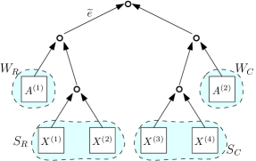
(a) Example of a possible execution tree $\mathcal{T}_{D}$. Given the choice of $e$ in the corresponding socket tree $\mathcal{T}_{S}$ shown on the right there are four possible choices of $\widetilde{e}$.

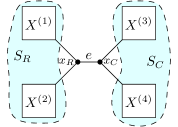
(b) The corresponding socket tree $\mathcal{T}_{S}$. The exact choice of $\widetilde{e}$ in $\mathcal{T}_{D}$ determines which part of the cut is the $x_{R}$ part, and which is the $x_{C}$ part.

Figure 1. Illustration of the notation used for the execution and socket trees.

Now, the tensor $P=T(D^{\prime}[W_{R}\cup S_{R}])$ appears as an intermediate result in the execution $\mathcal{T}_{D}$, hence the volume of $P$ is a lower bound on the cost of $\mathcal{T}_{D}$.

We group the modes of $D^{\prime}$ incident on $S_{R}$ or $W_{R}$ as shown in Figure 2: $E_{SW}$ are all modes in $D^{\prime}$ incident exactly upon $S_{R}$ and $W_{R}$, $E_{WC}$ are all modes incident on $W_{R}$ but not on $S_{R}$, $E_{SC}$ are all modes incident on $S_{R}$ but not $W_{R}$, and finally $E_{SWC}$ are all modes incident upon $S_{R}$, $W_{R}$, and at least one of $S_{C}$ or $W_{C}$. Write $E_{S}=E_{SW}\cup E_{SC}\cup E_{SWC}$ for the modes incident on $S_{R}$, and similarly $E_{C}=E_{WC}\cup E_{SC}\cup E_{SWC}$ for all modes incident upon at least one of $S_{R}$/$W_{R}$ and at least one of $S_{C}$/$W_{C}$. Note that $|J(E_{C})|$ is precisely the volume of $P$ which we aim to lower bound.

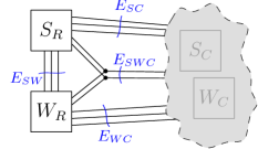
Figure 2. Illustration of $D^{\prime}$. We group the modes of $D^{\prime}$ based on how they connect $S_{R}$, $S_{C}$, and the “$C$ part” of $D^{\prime}$.

Define a matrix $A\in\mathbb{F}^{J(E_{S})}\times\mathbb{F}^{J(E_{C})}$ as follows. We identify its row indices $i\in J(E_{S})$ as being triples $i=(i_{SW},i_{SC},i_{SWC})\in J(E_{SW})\times J(E_{SC})\times J(E_{SWC})$ and similarly its column indices $j\in J(E_{C})$ are triples $j=(j_{SC},j_{WC},j_{SWC})\in J(E_{SC})\times J(E_{WC})\times J(E_{SWC})$. Then the entries of $A$ are

$$A_{(i_{SW},i_{SC},i_{SWC}),(j_{SC},j_{WC},j_{SWC})}=\begin{cases}T(D^{\prime}[W_{R}])_{i_{SW},j_{WC},j_{SWC}}&\!\!\text{if }i_{SC}=j_{SC}\wedge i_{SWC}=j_{SWC},\\ 0&\!\!\text{otherwise},\end{cases}$$

In the case when $E_{S}=E_{SW}$ (i.e., all modes incident on $S_{R}$ connect only to $W_{R}$), $A$ is simply a flattening of $T(D^{\prime}[W_{R}])$. Recall that $T(D^{\prime}[S_{R}])\in\prod_{e\in E_{S}}\mathbb{F}^{J(e)}$. Then for every $j=(j_{SC},j_{WC},j_{SWC})\in J(E_{C})$, we have

$$\sum_{i\in J(E_{S})}A_{i,j}T(D^{\prime}[S_{R}])_{i} =\sum_{i_{SW}\in J(E_{SW})}A_{(i_{SW},j_{SC},j_{SWC}),j}T(D^{\prime}[S_{R}])_{i_{SW},j_{SC},j_{SWC}}$$

$$=\sum_{i_{SW}}T(D^{\prime}[W_{R}])_{i_{SW},j_{WC},j_{SWC}}T(D^{\prime}[S_{R}])_{i_{SW},j_{SC},j_{SWC}}$$

$$=P_{j_{SC},j_{WC},j_{SWC}}=P_{j}$$

(recall that $P$ is the contraction of $T(D^{\prime}[W_{R}])$ and $T(D^{\prime}[S_{R}])$). Viewing $T(D^{\prime}[S_{R}])$ as a row vector in $\mathbb{F}^{J(E_{S})}$ we see that $P$ is simply the vector-matrix product $P=T(D^{\prime}[S_{R}])\cdot A\in\mathbb{F}^{J(E_{C})}$.

Symmetrically, for the other half of $D^{\prime}$, we can write $Q=T(D^{\prime}[W_{C}\cup S_{C}])$ as a matrix-vector product $Q=B\cdot T(D^{\prime}[S_{C}])\in\mathbb{F}^{J(E_{C})}$ where $B$ is a matrix corresponding to $T(D^{\prime}[W_{S}])$ analogously to how $A$ corresponds to $T(D^{\prime}[W_{R}])$.

Thus we have $T(D)=T(D^{\prime}[S_{R}])\cdot A\cdot B\cdot T(D^{\prime}[S_{C}])$. Recall that for each socket vertex $S_{i}$ in the original network $D$, we have $T(S_{i})=X^{(i)}$. Denoting $X_{R}=T(D^{\prime}[S_{R}])$ and $X_{C}=T(D^{\prime}[S_{C}])$, we get $X_{R}=\bigotimes_{S_{i}\in S_{R}}X^{(i)}$ and $X_{C}=\bigotimes_{S_{i}\in S_{C}}X^{(i)}$. Hence

$$F(X^{(1)},X^{(2)},\ldots,X^{(\ell)})=X_{R}\cdot A\cdot B\cdot X_{C}.$$

It follows that $A\cdot B$ is the flattening of $T(F)$ to a matrix with rows indexed by the sockets in $S_{R}$ and columns indexed by the sockets in $S_{C}$. But this flattening is precisely the matrix $M(\mathcal{T}_{S},e)$, implying that $|J(E_{C)}|\geq\operatorname{rk}(M(\mathcal{T}_{S},e))=w(\mathcal{T}_{S})$, as desired. ∎

7. Lower bounds for socket-width

In this section we establish lower bounds on socket-width for concrete maps.

7.1. Determinant and permanent

We now prove lower bounds for the socket width of the determinant and permanent. Let us start with the following trivial observation.

Claim 7.1.

For any socket tree $\mathcal{T}_{S}$ with $n\geq 2$ leaves, there is an edge $e=\{x_{R},x_{C}\}$ such that $n/3\leq|L(x_{R},e)|<2n/3$.

Proof.

Consider all edges $e=\{x_{R},x_{C}\}$ such that $|L(x_{R},e)|\geq n/3$. At least one such edge certainly exists since $n\geq 2$. Indeed, an edge $e=\{x_{R},x_{C}\}$ incident to a leaf $x_{C}$ has $|L(x_{R},e)|=n-1$ leaves. Among these, choose an edge such that $\mathcal{T}_{S}(x_{R},e)$ is of minimal size. Assume for contradiction that $|L(x_{R},e)|\geq 2n/3$. But then one of the two subtrees of $x_{R}$ in $\mathcal{T}_{S}(x_{R},e)$ must have at least $n/3$ leaves, and since they are smaller than $\mathcal{T}_{S}(x_{R},e)$, this contradicts the minimality of $\mathcal{T}_{S}(x_{R},e)$. ∎

Lemma 7.2.

For every positive integer $n\geq 2$, the socket-width of both the determinant and the permanent of an $n\times n$ matrix is at least $\binom{n}{\lceil n/3\rceil}$.

Proof.

Let $\mathcal{T}_{S}$ be a socket tree for the permanent, let $e=\{x_{R},x_{C}\}$ be an arbitrary edge in $\mathcal{T}_{S}$, and let $k=|L(x_{R},e)|$ be the number of leaves in $\mathcal{T}_{S}(x_{R},e)$. We now show that $\operatorname{rk}(M(\mathcal{T}_{S},e))\geq\binom{n}{k}$.

Recall that the sockets of $\mathcal{T}_{S}$ are the $n$ rows of the input matrix. Without loss of generality, number the rows so that the leaves of $\mathcal{T}_{S}(x_{R},e)$ are rows $1$ to $k$, and the leaves of $\mathcal{T}_{S}(x_{C},e)$ are rows $k+1$ to $n$. The rows of $M(\mathcal{T}_{S},e)$ are indexed by a tuple $j_{R}=(i_{1},\ldots,i_{k})\in[n]^{k}$, and the columns are indexed by a tuple $j_{C}=(i_{k+1},\ldots,i_{n})\in[n]^{n-k}$. The entry of $M(\mathcal{T}_{S},e)$ at position $(j_{R},j_{C})$ is $1$ if $(i_{1},i_{2},\ldots,i_{n})$ is a permutation. For any set $U\in\binom{[n]}{k}$, let $u_{1}<u_{2}<\ldots<u_{k}$ be the elements of $U$ in ascending order and define $j_{R}(U)=(u_{1},\ldots,u_{k})$; let $u_{k+1}<u_{k+2}<\ldots<u_{n}$ be the elements of $[n]\setminus U$ in ascending order and define $j_{C}(U)=(u_{k+1},u_{k+2},\ldots,u_{n})$.

For $U_{1},U_{2}\in\binom{[n]}{k}$, the entry of $M(\mathcal{T}_{S},e)$ at position $(j_{R}(U_{1}),j_{C}(U_{2}))$ equals $1$ if $U_{1}=U_{2}$, and $0$ otherwise. This induces a $\binom{n}{k}\times\binom{n}{k}$ identity submatrix of $M(\mathcal{T}_{S},e)$, implying $\operatorname{rk}(M(\mathcal{T}_{S},e))\geq\binom{n}{k}$.

By Claim 7.1, $\mathcal{T}_{S}$ has an edge $e$ with $n/3\leq k<2n/3$. For that edge, $\operatorname{rk}(M(\mathcal{T}_{S},e))\geq\binom{n}{k}\geq\binom{n}{\lceil n/3\rceil}$, which completes the proof for the permanent.

For the determinant, the only change is that some entries of $M(\mathcal{T}_{S},e)$ become $-1$ instead of $1$, but this only changes the identified submatrix from an identity matrix to a diagonal matrix and in particular does not change its rank. ∎

The preceding proof is similar to a lower bound by Nisan ([73], Lemma 2) used to obtain lower bounds for algebraic branching programs. But the lower bounds obtained there can be made as sharp as $\Omega(2^{n})$ whereas in our setting, we cannot rule out the possibility of a tensor network that avoids splitting the $n$ variables in two approximately equal size parts. This means that the best we can obtain with our current method is $\binom{n}{\lceil n/3\rceil}$ instead of $\binom{n}{n/2}$.

7.2. $P$-linear forms

Suppose $\mathcal{T}_{S}$ is a socket tree for a $P$-linear form for a $k$-uniform hypergraph $P$ on $v$ vertices. Recall that the sockets of this form correspond to the elements of $E(P)\subseteq\binom{[v]}{k}$. Given an edge $e\in E(\mathcal{T}_{S})$ and a vertex $x\in V(\mathcal{T}_{S})$, we write

$$U(x,e)=\bigcup_{S\in L(x,e)}S\subseteq[v].$$

Claim 7.3.

Let $\mathcal{T}_{S}$ be a socket tree for the $P$-linear form of order $n$. Let $e=\{x_{R},x_{C}\}\in E(\mathcal{T}_{S})$ and suppose $|U(x_{C},e)\cap U(x_{R},e)|=u$. Then the socket width of $\mathcal{T}_{S}$ is at least $w(\mathcal{T}_{S})\geq n^{u}$.

Proof.

Let $m=n^{u}$. We show that $\operatorname{rk}(M(\mathcal{T}_{S},e))\geq m$ by identifying an $m\times m$ identity submatrix of $M(\mathcal{T}_{S},e)$.

Define $E_{R}=\{\,(S,i)\,|\,S\in L(x_{R},e),i\in S\,\}$ to be the modes contained in the sockets on the $x_{R}$ side of $e$, and analogously $E_{C}=\{\,(S,i)\,|\,S\in L(x_{C},e),i\in S\,\}$.

The rows of $M(\mathcal{T}_{S},e)$ are indexed by $J(E_{R})$ and the columns are indexed by $J(E_{C})$. We will consider an $m\times m$ submatrix of $M(\mathcal{T}_{S},e)$ whose rows and columns are indexed by the elements $\sigma\in\prod_{i\in A}[n_{i}]$. More specifically, each row of the submatrix is indexed by $j_{R}$ where $j_{R}|_{(S,i)}=\sigma|_{i}$ for $i\in A$, and $j_{R}|_{(S,i)}=1$ for $i\not\in A$. Each column is indexed by $j_{C}$ where $j_{C}|_{(S,i)}=\sigma|_{i}$ for $i\in A$ and $j_{C}|_{(S,i)}=1$ for $i\not\in A$.

The value of the submatrix at position $(j_{R},j_{C})$ is $1$ if there exists $\sigma\in\prod_{i\in A}[n_{i}]$ such that $j_{R}|_{(S,i)}=\sigma|_{i}$ and $j_{C}|_{(S,i)}=\sigma|_{i}$ for all $i\in A$ and $0$ otherwise. We obtain an $m\times m$ identity matrix as desired. ∎

From this claim, the branchwidth-based lower bound is immediate.

Lemma 7.4.

For any hypergraph $P$, the socket width of the $P$-linear form of order $n$ is at least $n^{\operatorname{bw}(P)}$.

Proof.

Any socket tree for a $P$-linear form can be directly viewed as a branch decomposition of $P$. Thus, by definition every socket tree for the form has an edge $e=\{x_{R},x_{C}\}$ where $|U(x_{C},e)\cap U(x_{R},e)|\geq\operatorname{bw}(P)$, and the lemma now follows from 7.3. ∎

For counting homomorphisms of hypergraph cliques, that is, the $P$-linear form for the complete $k$-uniform hypergraph $P=\binom{[v]}{k}$ on $v$ vertices, we need the following simple lower bound on the branchwidth of complete hypergraphs (which is most likely known, but we are not aware of a reference).

Lemma 7.5.

For $v>k\geq 3$, the complete $k$-uniform hypergraph on $v$ vertices has branchwidth $v$.

Proof.

Let $T$ be an arbitrary branch decomposition of the hypergraph.

First, we note that for every edge $e=\{x_{R},x_{C}\}$, either $U(x_{R},e)=[v]$ or $U(x_{C},e)=[v]$. Indeed, suppose for contradiction that there is an edge $e=\{x_{R},x_{C}\}$ with $i_{1}\not\in U(x_{R},e)$ and $i_{2}\not\in U(x_{C},e)$ for some not necessarily distinct $i_{1},i_{2}\in[v]$. Since $k\geq 2$, there exists an edge $S\supseteq\{i_{1},i_{2}\}$, and that edge must appear in either $\mathcal{T}_{S}(x_{R},e)$ or $\mathcal{T}_{S}(x_{C},e)$.

Now, if $U(x_{R},e)=U(x_{C},e)=[v]$ for some $e=\{x_{R},x_{C}\}$, then we are done, so suppose for contradiction that this is not the case. Direct each edge towards the subtree which covers $[v]$. For example, if $U(x_{R},e)=[v]$ and $U(x_{C},e)\neq[v]$ then $e$ is directed towards $x_{R}$.

Since a tree is acyclic, there must be some vertex $x^{*}$ such that all edges incident to $x^{*}$ are directed towards $x^{*}$. The vertex $x^{*}$ cannot be a leaf, because the subtree consisting of a leaf contains a single edge, which covers $k<v$ elements. Thus $x^{*}$ has degree $3$. Let the three edges incident to $x^{*}$ be $e_{1}=\{x^{*},y_{1}\}$, $e_{2}=\{x^{*},y_{2}\}$ and $e_{3}=\{x^{*},y_{3}\}$. Since all the edges are directed towards $x^{*}$ there are $i_{1},i_{2},i_{3}\in[v]$ such that $i_{1}\not\in S(y_{1},e_{1})$, $i_{2}\not\in S(y_{2},e_{2})$ and $i_{3}\not\in S(y_{3},e_{3})$. Since $k\geq 3$ there exists a edge $S\supseteq\{i_{1},i_{2},i_{3}\}$. But now the edge $S$ cannot appear in any of the subtrees rooted at $y_{1}$, $y_{2}$, or $y_{3}$. Since these three subtrees together cover all leaves, this yields the desired contradiction and we conclude that there must exist an edge $e$ such that $U(x_{R},e)=U(x_{C},e)=[v]$ and therefore the branchwidth is $v$. ∎

7.3. Kruskal operator

We say that an $\ell$-linear Kruskal operator is $n$-uniform if the lengths of the modes satisfy $n=n_{1}=n_{2}=\cdots=n_{\ell}$.

Lemma 7.6.

For positive integers $n$ and $r$, the socket-width of an $n$-uniform $\ell$-linear Kruskal operator is at least $\max\left(n^{\ell},n^{\lceil\ell/2\rceil}r\right)$.

Proof.

Let $\mathcal{T}_{S}$ be an arbitrary socket tree for the operator. One of the leaves is the output socket representing the tensor $B$ of shape $n\times n\times\cdots\times n$ ($\ell$ times) that is obtained by applying the Kruskal operator to the input matrices $A^{(i)}$ of shape $n\times r$, where $1\leq i\leq\ell$.

Consider the neighbor $x$ of the output socket. It has three neighbors: the output socket leaf, and two other vertices $x_{R}$ and $x_{C}$. Either the subtree rooted at $x_{R}$ or the one rooted at $x_{C}$ must contain $u\geq\lceil\ell/2\rceil$ input sockets (since together they contain all $\ell$ input sockets). Let $e$ be the edge leading to that subtree.

We claim that $\operatorname{rk}(M(\mathcal{T}_{S},e))\geq n^{u}r$. Suppose without loss of generality that the input sockets $A^{(1)},\ldots,A^{(u)}$ are in the subtree rooted at $x_{R}$, and that the input sockets $A^{(u+1)},\ldots,A^{(\ell)}$ are in the subtree rooted at $x$ together with the output socket.

Each row of $M(\mathcal{T}_{S},e)$ is indexed by sequences of $2u$ indices $(i_{1},j_{1},\ldots,i_{u},j_{u})$ where each $i\in[n]$ and each $j\in[r]$. Each column is indexed by a sequence of $\ell+2(n-u)$ indices $(i_{1}^{\prime},\ldots,i_{\ell}^{\prime};$ $i_{u+1},j_{u+1},\ldots,i_{\ell},j_{\ell})$ where each $i,i^{\prime}\in[n]$ and each $j\in[r]$. An entry of $M(\mathcal{T}_{S},e)$ is $1$ if and only if $i_{1}^{\prime}=i_{1},i_{2}^{\prime}=i_{2},\ldots,i_{\ell}^{\prime}=i_{\ell}$, and $j_{1}=j_{2}=\ldots=j_{\ell}$.

For any $i_{1},\ldots,i_{u}\in[n]$ and $j\in[r]$, consider the row index $(i_{1},j,i_{2},j,\ldots,i_{u},j)$ and the column index $(i_{1},i_{2},\ldots,i_{u},1,1,\ldots,1;1,j,1,j,\ldots,1,j)$. The $n^{u}r\times n^{u}r$ submatrix of $M(\mathcal{T}_{S},e)$ induced by these sets of row and column indices is the identity matrix, thus $\operatorname{rk}(M(\mathcal{T}_{S},e))\geq n^{u}r$ as desired.

For the $n^{\ell}$ lower bound, we instead consider the edge $e^{\prime}$ joining $x$ with the output socket. Now the rows are indexed by $(i_{1},j_{1},i_{2},j_{2},\ldots,i_{\ell},j_{\ell})$ and the columns by $(i_{1}^{\prime},\ldots,i_{\ell}^{\prime})$. The $n^{\ell}\times n^{\ell}$ identity submatrix is obtained by taking for every $i_{1},\ldots,i_{\ell}\in[n]$, the row $(i_{1},1,i_{2},1,\ldots,i_{\ell},1)$ and the column $(i_{1},\ldots,i_{\ell})$. ∎

Appendix A Minimum-cost execution

This appendix summarizes some results on tensor network contractions and minimum-cost executions. These results are not original work, but for the sake of completeness we present them here.

A.1. Invariance property

In the following lemma, we will show that the tensor of a network is equal to the tensor of any network that is obtained by a contraction from the original network. In particular, this implies that any execution gives the same tensor.

Lemma A.1 (Invariance).

Let $D$ be a tensor network. For all nonempty $W\subseteq V(D)$ it holds that $T(D)=T(D/W)$.

Proof.

Let $W\subseteq V(D)$ be nonempty and let $i\in J(B(D/W))=J(B(D))$. From (23), (24), and (25), it follows that

$$\begin{split}T(D/W)_{i}&=\sum_{j\in J(E(D/W)\setminus B(D/W))}\prod_{v\in(V(D)\setminus W)\cup\{w\}}T(v)_{ij}\\ &=\sum_{j\in J(E(D/W)\setminus B(D/W))}T(w)_{ij}\prod_{v\in V(D)\setminus W}T(v)_{ij}\\ &=\sum_{j\in J(E(D/W)\setminus B(D))}T(D[W])_{ij}\prod_{v\in V(D)\setminus W}T(v)_{ij}\\ &=\sum_{j\in J(E(D/W)\setminus B(D))}\ \sum_{j^{\prime}\in J(E(D[W])\setminus B(D[W]))}\ \prod_{w\in W}T(w)_{ijj^{\prime}}\prod_{v\in V(D)\setminus W}T(v)_{ij}\\ &=\sum_{j\in J(E(D/W)\setminus B(D))}\ \sum_{j^{\prime}\in J(E(D[W])\setminus B(D[W]))}\ \prod_{v\in V(D)}T(v)_{ijj^{\prime}}\\ &=\sum_{j^{\prime\prime}\in J(E(D)\setminus B(D))}\ \prod_{v\in V(D)}T(v)_{ij^{\prime\prime}}\\ &=T(D)_{i}\,.\end{split}$$

∎

A.2. The structure of a minimum-cost execution

In this section, we analyze the structure of a minimum-cost execution. In particular, we will prove Lemma 4.1 that states that each contracted set has size at most two and also show that one can always contract adjacent vertices in a network.

See 4.1

Proof.

If $D$ contains loops, we may assume that a minimum-cost execution first removes all the loops by contracting singleton vertices incident to loops. Indeed, the cost of contracting a singleton vertex is the volume of the tensor associated to it. Since the result of an execution is a single tensor, then every vertex has to be contained in a contracted set of an execution and none of the hyperedges incident to a vertex cannot be removed before the vertex is contained in a contracted set. Hence, the volume of any tensor in the tensor network is a lower bound for the cost of any execution of $D$ and we may contract singleton vertices.

So let us assume that $D$ is loopless. Suppose that a minimum-cost execution of $D$ contains a contraction by a set $W=\{w_{1},w_{2},\ldots,w_{s}\}$ of size at least $s\geq 3$, and let $w$ be the new vertex after this contraction. Then we can replace the contraction by $W$ with two contractions by $W^{\prime}=\{w_{1},w_{2},\ldots,w_{s-1}\}$ and $W^{\prime\prime}=\{w,w_{s}\}$ without increasing the cost of the execution. The cost of contracting $W^{\prime}$ is less or equal than the cost of contracting $W$, because every hyperedge incident to $W^{\prime}$ is also incident to $W$. The cost of contracting $W^{\prime\prime}$ is less or equal than the cost of contracting $W$, because the set of hyperedges incident to $w$ is contained in the set of hyperedges incident to $W^{\prime}$. We repeat this procedure until all contracted sets in the execution have size at most two. ∎

Two tensors in a tensor network are called adjacent if they are incident to a common mode.

Lemma A.2 (Execution by contracting adjacent tensors).

Let $D$ be a loopless tensor network that is connected as a hypergraph. Then, there exists a minimum-cost execution of $D$ such that each contracted set has size two and consists of adjacent vertices.

Proof.

Consider a minimum-cost execution of $D$ such that each contracted set has size two; such an execution exists by Lemma 4.1. If all contracted sets in the execution consist of adjacent vertices, we are done. Otherwise, consider a contraction of two vertices, $u$ and $v$, such that $u$ and $v$ are not adjacent when they are contracted to yield the vertex $uv$. Consider the steps of the execution after this contraction step. Let us call such a step a relevant step if it involves a descendant of the vertex $uv$. Let us modify the execution as follows. First, delete the contraction of $u$ and $v$ from the execution. Then, for each relevant step in execution order, replace the descendant of the vertex $uv$ with the current descendant of either $u$ or $v$ so that the contraction becomes a contraction of adjacent vertices whenever possible. If the descendants of $u$ and $v$ become adjacent after a relevant step, contract the descendants of $u$ and $v$, and then continue the execution without further changes. Since $D$ is connected, the descendants of $u$ and $v$ must eventually become adjacent.

We will show that this modification of the execution gives again an execution and that it has cost no larger than the original minimum-cost execution. In the modification of the execution, let the contraction sets containing $u$ or a descendant of $u$ and not containing a descendant of $v$ be $\{u,w_{1}\},\{uw_{1},w_{2}\}$, $\ldots$, $\{uw_{1}\ldots w_{s-1},w_{s}\}$; similarly, let the contraction sets containing $v$ or a descendant of $v$ and not containing a descendant of $u$ be $\{v,z_{1}\}$, $\{vz_{1},z_{2}\},\ldots$, $\{vz_{1}\ldots z_{t-1},z_{t}\}$. Here $w_{1},\ldots,w_{s},z_{1},\ldots,z_{t}$ can be vertices of $D$ or vertices obtained after contraction steps. Contracting $\{uw_{1}\ldots w_{s},vz_{1}\ldots z_{t}\}$ gives the vertex $uw_{1}\ldots w_{s}vz_{1}\ldots z_{t}$, which appears also in the original execution. Hence, after certain steps the tensor networks in the original execution and in the modification are the same (after making necessary non-relevant contractions) and the modification of the original execution is also an execution.

First we consider the cost of contracting $\{uw_{1}\ldots w_{i-1},w_{i}\}$ in the modified execution where $1\leq i\leq s$. There exists a $j$ satisfying $1\leq j\leq t$ such that in the original execution we contract $\{uw_{1}\ldots w_{i-1}vz_{1}\ldots z_{j},w_{i}\}$. Then the cost of contracting $\{uw_{1}\ldots w_{i-1},w_{i}\}$ is less or equal that the cost of contracting $\{uw_{1}\ldots w_{i-1}vz_{1}\ldots z_{j},w_{i}\}$, because every hyperedge incident to the vertex $uw_{1}\ldots w_{i-1}$ in the modified execution has to be incident to $uw_{1}\ldots w_{i-1}vz_{1}\ldots z_{j}$ in the original execution. Otherwise, there would be an hyperedge in $D$ that is incident only to vertices in $\{u,w_{1},\ldots,w_{i-1},v,z_{1},\ldots,z_{j}\}$, and in particular both to vertices in $\{u,w_{1},\ldots,w_{i-1}\}$ and in $\{v,z_{1},\ldots,z_{j}\}$. This is impossible, because then $uw_{1}\ldots w_{i-1}$ and $vz_{1}\ldots z_{j}$ would be adjacent vertices in the modified execution, but by assumption $uw_{1}\ldots w_{s}$ and $vz_{1}\ldots z_{t}$ are the first adjacent descendants of $u$ and $v$ in the modified execution. Similarly, we can show that the cost of contracting $\{vz_{1}\ldots z_{j-1},z_{j}\}$ in the modified execution for $1\leq j\leq t$ is less than the cost of contracting a set in the original execution.

Second we consider the cost of contracting $\{uw_{1}\ldots w_{s},vz_{1}\ldots z_{t}\}$ in the modified execution. Without loss of generality, we can assume that in the original execution the vertex $uw_{1}\ldots w_{s}vz_{1}\ldots z_{t}$ is obtained from contracting $\{uw_{1}\ldots w_{s}vz_{1}\ldots z_{t-1},z_{t}\}$. We will show that the cost of contracting $\{uw_{1}\ldots w_{s},vz_{1}\ldots z_{t}\}$ in the modified execution is less or equal than the cost of contracting $\{uw_{1}\ldots w_{s}vz_{1}\ldots z_{t-1},z_{t}\}$ in the original execution. Indeed, every hyperedge incident to $uw_{1}\ldots w_{s}$ in the modified execution is incident to $uw_{1}\ldots w_{s}vz_{1}\ldots z_{t-1}$ in the original execution, because otherwise there would be an hyperedge in $D$ that is incident only to vertices in $\{u,w_{1},\ldots,w_{s},v,z_{1},\ldots,z_{t-1}\}$, and in particular both to vertices in $\{u,w_{1},\ldots,w_{s}\}$ and $\{v,z_{1},\ldots,z_{t-1}\}$. However, by assumption $uw_{1}\ldots w_{s}$ and $vz_{1}\ldots z_{t}$ are the first adjacent descendants of $u$ and $v$ in the modified execution. Similarly, every hyperedge incident to $vz_{1}\ldots z_{t}$ in the modified execution is incident to $uw_{1}\ldots w_{s}vz_{1}\ldots z_{t-1}$ or $z_{t}$ in the original execution, because otherwise there would be an hyperedge in $D$ that is incident only to vertices in $\{u,w_{1},\ldots,w_{s},v,z_{1},\ldots,z_{t-1}\}$, and in particular both to vertices in $\{u,w_{1},\ldots,w_{s}\}$ and $\{v,z_{1},\ldots,z_{t-1}\}$. This contradicts that $uw_{1}\ldots w_{s}$ and $vz_{1}\ldots z_{t}$ are the first adjacent descendants of $u$ and $v$ in the modified execution.

The modified execution consists of at least one less contraction of nonadjacent vertices. Repeating this procedure until there are no contractions of nonadjacent vertices completes the lemma. ∎

A.3. Finding a minimum-cost execution

In this section, we will show a recurrence relation for the cost of a tensor network. To this end, let $D$ be a loopless connected tensor network $D$ with at least two tensors. Let us write $\mathscr{C}(D)$ for the set of all $W\subseteq V(D)$ such that $D[W]$ is connected.

Lemma A.3.

Let $D$ be a loopless connected tensor network $D$ with at least two tensors. The cost of $D$ satisfies the recurrence

$$c(D)=\!\!\!\!\min_{\begin{subarray}{c}W\in\mathscr{C}(D)\\ V(D)\setminus W\in\mathscr{C}(D)\end{subarray}}\!\!\!\!\max\bigl{(}c(D[W]),c(D[V(D)\setminus W]),c(D/W/(V(D)\setminus W))\bigr{)}\,.$$ (47)

Proof.

We recall that the cost $c(D)$ of $D$ is the cost of minimum-cost execution of $D$. We can view a minimum-cost execution of $D$ as a rooted tree such that the root has degree two, all non-root internal vertices have degree three, and each leaf vertex is a tensor of $D$. By Lemma A.2, the two subtrees rooted at the neighbours of the root define two disjoint sets $U,W\subseteq V(D)$ such that $U\cup W=V(D)$ and both $D[U]$ and $D[W]$ are connected. The cost of the contraction at the root is $c(D/W/U)$, and the subtrees rooted at $U$ and $W$ cost $c(D[U])$ and $c(D[W])$, respectively. The recurrence considers all the partitions to connected sets, including the optimum. ∎

References

- [1] Amir Abboud, Arturs Backurs, Karl Bringmann, and Marvin Künnemann. Fine-grained complexity of analyzing compressed data: Quantifying improvements over decompress-and-solve. In Proc. of Foundations of Computer Science (FOCS), pages 192–203, 2017. doi:10.1109/FOCS.2017.26.
- [2] Amir Abboud, Arturs Backurs, and Virginia Vassilevska Williams. If the current clique algorithms are optimal, so is Valiant’s parser. In Proc. of Foundations of Computer Science (FOCS), pages 98–117, 2015. doi:10.1109/FOCS.2015.16.
- [3] Michael Alekhnovich, Allan Borodin, Joshua Buresh-Oppenheim, Russell Impagliazzo, Avner Magen, and Toniann Pitassi. Toward a model for backtracking and dynamic programming. Comput. Complex., 20(4):679–740, 2011. doi:10.1007/s00037-011-0028-y.
- [4] Noga Alon and Shai Gutner. Balanced families of perfect hash functions and their applications. ACM Trans. Algorithms, 6(3):54:1–54:12, 2010. doi:10.1145/1798596.1798607.
- [5] Noga Alon, Raphael Yuster, and Uri Zwick. Finding and counting given length cycles. Algorithmica, 17(3):209–223, 1997. doi:10.1007/BF02523189.
- [6] Itai Arad and Zeph Landau. Quantum computation and the evaluation of tensor networks. SIAM J. Comput., 39(7):3089–3121, 2010. doi:10.1137/080739379.
- [7] Sanjeev Arora and Boaz Barak. Computational Complexity: A Modern Approach. Cambridge University Press, New York, NY, USA, 1st edition, 2009. doi:10.1017/CBO9780511804090.
- [8] Fahiem Bacchus, Shannon Dalmao, and Toniann Pitassi. Algorithms and complexity results for #SAT and Bayesian inference. In Proc. of Foundations of Computer Science (FOCS), pages 340–351, 2003. doi:10.1109/SFCS.2003.1238208.
- [9] Martin Beaudry and Markus Holzer. The complexity of tensor circuit evaluation. Comput. Complex., 16(1):60–111, 2007. doi:10.1007/s00037-007-0222-0.
- [10] Austin R. Benson and Grey Ballard. A framework for practical parallel fast matrix multiplication. In Proc. of Principles and Practice of Parallel Programming (PPoPP), pages 42–53, 2015. doi:10.1145/2688500.2688513.
- [11] Stuart J. Berkowitz. On computing the determinant in small parallel time using a small number of processors. Inf. Process. Lett., 18(3):147–150, 1984. doi:10.1016/0020-0190(84)90018-8.
- [12] Jacob D. Biamonte, Jason Morton, and Jacob Turner. Tensor network contractions for #SAT. J. Stat. Phys., 160(5):1389–1404, 2015. doi:10.1007/s10955-015-1276-z.
- [13] Andreas Björklund. Below all subsets for some permutational counting problems. In Proc. of Scandinavian Symposium and Workshops on Algorithm Theory (SWAT), pages 17:1–17:11, 2016. doi:10.4230/LIPIcs.SWAT.2016.17.
- [14] Andreas Björklund, Thore Husfeldt, Petteri Kaski, and Mikko Koivisto. Fourier meets Möbius: fast subset convolution. In Proc. of Symposium on Theory of Computing (STOC), pages 67–74, 2007. doi:10.1145/1250790.1250801.
- [15] Andreas Björklund, Thore Husfeldt, Petteri Kaski, and Mikko Koivisto. Computing the Tutte polynomial in vertex-exponential time. In Proc. of Foundations of Computer Science (FOCS), pages 677–686, 2008. doi:10.1109/FOCS.2008.40.
- [16] Andreas Björklund, Thore Husfeldt, Petteri Kaski, and Mikko Koivisto. Counting paths and packings in halves. In Proc. of European Symposium on Algorithms (ESA), pages 578–586, 2009. doi:10.1007/978-3-642-04128-0_52.
- [17] Andreas Björklund, Thore Husfeldt, and Mikko Koivisto. Set partitioning via inclusion-exclusion. SIAM J. Comput., 39(2):546–563, 2009. doi:10.1137/070683933.
- [18] Andreas Björklund, Petteri Kaski, and Łukasz Kowalik. Counting thin subgraphs via packings faster than meet-in-the-middle time. In Proc. of Symposium on Discrete Algorithms (SODA), pages 594–603, 2014. doi:10.1137/1.9781611973402.45.
- [19] Hans L. Bodlaender, Erik Jan van Leeuwen, Johan M. M. van Rooij, and Martin Vatshelle. Faster algorithms on branch and clique decompositions. In Proc. of Mathematical Foundations of Computer Science (MFCS), pages 174–185, 2010. doi:10.1007/978-3-642-15155-2_17.
- [20] James R. Bunch and John E. Hopcroft. Triangular factorization and inversion by fast matrix multiplication. Math. Comp., 28:231–236, 1974. doi:10.2307/2005828.
- [21] Peter Bürgisser, Michael Clausen, and M. Amin Shokrollahi. Algebraic Complexity Theory. Springer-Verlag, Berlin, 1997. doi:10.1007/978-3-662-03338-8.
- [22] Jin-Yi Cai, Heng Guo, and Tyson Williams. A complete dichotomy rises from the capture of vanishing signatures. SIAM J. Comput., 45(5):1671–1728, 2016. doi:10.1137/15M1049798.
- [23] Jin-yi Cai, Pinyan Lu, and Mingji Xia. Computational complexity of holant problems. SIAM J. Comput., 40(4):1101–1132, 2011. doi:10.1137/100814585.
- [24] Florent Capelli, Arnaud Durand, and Stefan Mengel. The arithmetic complexity of tensor contraction. Theory Comput. Syst., 58(4):506–527, 2016. doi:10.1007/s00224-015-9630-8.
- [25] A. Cayley. On the theory of the analytical forms called trees. Philos. Mag., 13:172–176, 1857. doi:10.1080/14786445708642275.
- [26] A. Cayley. On the analytical forms called trees, part II. Philos. Mag., 18:374–378, 1859. doi:10.1080/14786445908642782.
- [27] Andrzej Cichocki, Namgil Lee, Ivan V. Oseledets, Anh Huy Phan, Qibin Zhao, and Danilo P. Mandic. Tensor networks for dimensionality reduction and large-scale optimization: Part 1 Low-rank tensor decompositions. Found. Trends Mach. Learn., 9(4-5):249–429, 2016. doi:10.1561/2200000059.
- [28] Andrzej Cichocki, Anh Huy Phan, Qibin Zhao, Namgil Lee, Ivan V. Oseledets, Masashi Sugiyama, and Danilo P. Mandic. Tensor networks for dimensionality reduction and large-scale optimization: Part 2 Applications and future perspectives. Found. Trends Mach. Learn., 9(6):431–673, 2017. doi:10.1561/2200000067.
- [29] A. Clebsch. Ueber symbolische Darstellung algebraischer Formen. J. Reine Angew. Math., 59:1–62, 1861. doi:10.1515/crll.1861.59.1.
- [30] W. Clifford. Extract of a letter to Mr. Sylvester from Prof. Clifford of University College, London. Amer. J. Math., 1(2):126–128, 1878. doi:10.2307/2369303.
- [31] Henry Cohn, Robert D. Kleinberg, Balázs Szegedy, and Christopher Umans. Group-theoretic algorithms for matrix multiplication. In Proc. of Foundations of Computer Science (FOCS), pages 379–388, 2005. doi:10.1109/SFCS.2005.39.
- [32] Henry Cohn and Christopher Umans. Fast matrix multiplication using coherent configurations. In Proc. of Symposium on Discrete Algorithms (SODA), pages 1074–1087, 2013. doi:10.1137/1.9781611973105.77.
- [33] James W. Cooley and John W. Tukey. An algorithm for the machine calculation of complex Fourier series. Math. Comp., 19:297–301, 1965. doi:10.2307/2003354.
- [34] Radu Curticapean, Holger Dell, and Dániel Marx. Homomorphisms are a good basis for counting small subgraphs. In Proc. of Symposium on Theory of Computing (STOC), pages 210–223, 2017. doi:10.1145/3055399.3055502.
- [35] Predrag Cvitanović. Group theory for Feynman diagrams in non-Abelian gauge theories. Phys. Rev. D, 14:1536–1553, 09 1976. doi:10.1103/PhysRevD.14.1536.
- [36] Predrag Cvitanović and A. D. Kennedy. Spinors in negative dimensions. Phys. Scr., 26(1):5–14, 1982. doi:10.1088/0031-8949/26/1/001.
- [37] Carsten Damm, Markus Holzer, and Pierre McKenzie. The complexity of tensor calculus. Comput. Complex., 11(1-2):54–89, 2002. doi:10.1007/s00037-000-0170-4.
- [38] Sashka Davis and Russell Impagliazzo. Models of greedy algorithms for graph problems. Algorithmica, 54(3):269–317, 2009. doi:10.1007/s00453-007-9124-4.
- [39] Josep Díaz, Maria J. Serna, and Dimitrios M. Thilikos. Counting H-colorings of partial k-trees. Theor. Comput. Sci., 281(1-2):291–309, 2002. doi:10.1016/S0304-3975(02)00017-8.
- [40] Frederic Dorn. Dynamic programming and fast matrix multiplication. In Proc. of European Symposium on Algorithms (ESA), pages 280–291, 2006. doi:10.1007/11841036_27.
- [41] Friedrich Eisenbrand and Fabrizio Grandoni. On the complexity of fixed parameter clique and dominating set. Theoret. Comput. Sci., 326(1-3):57–67, 2004. doi:10.1016/j.tcs.2004.05.009.
- [42] Norman P. Jouppi et al. In-datacenter performance analysis of a tensor processing unit. In Proc. of International Symposium on Computer Architecture (ISCA), pages 1–12, 2017. doi:10.1145/3079856.3080246.
- [43] Peter Floderus, Miroslaw Kowaluk, Andrzej Lingas, and Eva-Marta Lundell. Detecting and counting small pattern graphs. SIAM J. Discrete Math., 29(3):1322–1339, 2015. doi:10.1137/140978211.
- [44] Fedor V. Fomin, Daniel Lokshtanov, Venkatesh Raman, Saket Saurabh, and B. V. Raghavendra Rao. Faster algorithms for finding and counting subgraphs. J. Comput. Syst. Sci., 78(3):698–706, 2012. doi:10.1016/j.jcss.2011.10.001.
- [45] William I. Gasarch. The Second P =? NP Poll. SIGACT News Complexity Theory Column, 74, 2012. doi:10.1145/2261417.2261434.
- [46] Johan Håstad. Tensor rank is NP-complete. J. Algorithm., 11(4):644–654, 1990. doi:10.1016/0196-6774(90)90014-6.
- [47] Christopher J. Hillar and Lek-Heng Lim. Most tensor problems are NP-hard. J. ACM, 60(6):45:1–45:39, 2013. doi:10.1145/2512329.
- [48] Jianyu Huang, Leslie Rice, Devin A. Matthews, and Robert A. van de Geijn. Generating families of practical fast matrix multiplication algorithms. In Proc. of International Parallel and Distributed Processing Symposium (IPDPS), pages 656–667, 2017. doi:10.1109/IPDPS.2017.56.
- [49] Russell Impagliazzo and Ramamohan Paturi. On the complexity of -SAT. J. Comput. Syst. Sci., 62(2):367–375, 2001. doi:10.1006/jcss.2000.1727.
- [50] Russell Impagliazzo, Ramamohan Paturi, and Francis Zane. Which problems have strongly exponential complexity? J. Comput. Syst. Sci., 63(4):512–530, 2001. doi:10.1006/jcss.2001.1774.
- [51] Alon Itai and Michael Rodeh. Finding a minimum circuit in a graph. SIAM J. Comput., 7(4):413–423, 1978. doi:10.1137/0207033.
- [52] Matti Karppa, Petteri Kaski, and Jukka Kohonen. A faster subquadratic algorithm for finding outlier correlations. ACM Trans. Algorithms, 14(3):31:1–31:26, 2018. doi:10.1145/3174804.
- [53] L. H. Kauffman. Knots, abstract tensors and the Yang-Baxter equation. In Knots, topology and quantum field theories, pages 179–334. 1989.
- [54] A. B. Kempe. On the application of Clifford’s graphs to ordinary binary quantics. P. Lond. Math. Soc., 17:107–121, 1885/86. doi:10.1112/plms/s1-17.1.107.
- [55] A. B. Kempe. On the application of the Sylvester-Clifford graphs to ordinary binary quantics. (Second part.). P. Lond. Math. Soc., 24:97–118, 1892/93. doi:10.1112/plms/s1-24.1.97.
- [56] Ton Kloks, Dieter Kratsch, and Haiko Müller. Finding and counting small induced subgraphs efficiently. Inf. Process. Lett., 74(3-4):115–121, 2000. doi:10.1016/S0020-0190(00)00047-8.
- [57] Tamara G. Kolda. Multilinear operators for higher-order decompositions. Technical Report SAND2006-2081, Sandia National Laboratories, 2006. doi:10.2172/923081.
- [58] Tamara G. Kolda and Brett W. Bader. Tensor decompositions and applications. SIAM Rev., 51(3):455–500, 2009. doi:10.1137/07070111X.
- [59] Daphne Koller and Nir Friedman. Probabilistic Graphical Models. Adaptive Computation and Machine Learning. MIT Press, Cambridge, MA, 2009.
- [60] Joseph B. Kruskal. Three-way arrays: rank and uniqueness of trilinear decompositions, with application to arithmetic complexity and statistics. Linear Algebra Appl., 18(2):95–138, 1977. doi:10.1016/0024-3795(77)90069-6.
- [61] Greg Kuperberg. Involutory Hopf algebras and -manifold invariants. Internat. J. Math., 2(1):41–66, 1991. doi:10.1142/S0129167X91000053.
- [62] Chi-Chung Lam, P. Sadayappan, and Rephael Wenger. On optimizing a class of multi-dimensional loops with reduction for parallel execution. Parallel Process. Lett., 7(2):157–168, 1997. doi:10.1142/S0129626497000176.
- [63] J. M. Landsberg. Tensors: Geometry and Applications, volume 128 of Graduate Studies in Mathematics. American Mathematical Society, Providence, RI, 2012. doi:10.1090/gsm/128.
- [64] Joseph M. Landsberg, Yang Qi, and Ke Ye. On the geometry of tensor network states. Quantum Inf. Comput., 12(3-4):346–354, 2012.
- [65] François Le Gall and Florent Urrutia. Improved rectangular matrix multiplication using powers of the Coppersmith-Winograd tensor. In Symposium on Discrete Algorithms, SODA 2018, pages 1029–1046, 2018. doi:10.1137/1.9781611975031.67.
- [66] François Le Gall. Faster algorithms for rectangular matrix multiplication. In Proc. of Foundations of Computer Science (FOCS), pages 514–523, 2012. doi:10.1109/FOCS.2012.80.
- [67] François Le Gall. Powers of tensors and fast matrix multiplication. In Proc. of International Symposium on Symbolic and Algebraic Computation (ISSAC), pages 296–303, 2014. doi:10.1145/2608628.2608664.
- [68] James R. Lee, Prasad Raghavendra, and David Steurer. Lower bounds on the size of semidefinite programming relaxations. In Proc. of Symposium on Theory of Computing (STOC), pages 567–576, 2015. doi:10.1145/2746539.2746599.
- [69] Andrea Lincoln, Virginia Vassilevska Williams, and R. Ryan Williams. Tight hardness for shortest cycles and paths in sparse graphs. In Proc. of Symposium on Discrete Algorithms (SODA), pages 1236–1252, 2018. doi:10.1137/1.9781611975031.80.
- [70] Stefano Markidis, Steven Wei Der Chien, Erwin Laure, Ivy Bo Peng, and Jeffrey S. Vetter. NVIDIA tensor core programmability, performance & precision. In Proc. of International Parallel and Distributed Processing Symposium Workshops (IPDPS), pages 522–531, 2018. doi:10.1109/IPDPSW.2018.00091.
- [71] Ankur Moitra and Alexander S. Wein. Spectral methods from tensor networks. arXiv:1811.00944, 2018. URL: http://arxiv.org/abs/1811.00944, arXiv:1811.00944.
- [72] J. Nešetřil and S. Poljak. On the complexity of the subgraph problem. Comment. Math. Univ. Carolin., 26(2):415–419, 1985.
- [73] Noam Nisan. Lower bounds for non-commutative computation (extended abstract). In Proc. of Symposium on Theory of Computing (STOC), pages 410–418, 1991. doi:10.1145/103418.103462.
- [74] Stephan Olariu. Paw-free graphs. Inf. Process. Lett., 28(1):53–54, 1988. doi:10.1016/0020-0190(88)90143-3.
- [75] R. Orús. A practical introduction to tensor networks: Matrix product states and projected entangled pair states. Ann. Phys., 349:117–158, 2014. doi:10.1016/j.aop.2014.06.013.
- [76] Victor Y. Pan. Matrix multiplication, trilinear decompositions, APA algorithms, and summation. arXiv:1412.1145, 2014.
- [77] Roger Penrose. Tensor Methods in Algebraic Geometry. PhD thesis, St. John’s College, 1956.
- [78] Roger Penrose. Applications of negative dimensional tensors. In Combinatorial Mathematics and its Applications, pages 221–244. 1971.
- [79] Roger Penrose and Wolfgang Rindler. Spinors and space-time. Vol. 1. Cambridge Monographs on Mathematical Physics. Cambridge University Press, Cambridge, 1984. doi:10.1017/CBO9780511564048.
- [80] Robert N. C. Pfeifer, Jutho Haegeman, and Frank Verstraete. Faster identification of optimal contraction sequences for tensor networks. Phys. Rev. E, 90:033315, 2014. doi:10.1103/PhysRevE.90.033315.
- [81] Ran Raz. Tensor-rank and lower bounds for arithmetic formulas. J. ACM, 60(6):40:1–40:15, 2013. doi:10.1145/2535928.
- [82] Jürgen Richter-Gebert and Peter Lebmeir. Diagrams, tensors and geometric reasoning. Discrete Comput. Geom., 42(2):305–334, 2009. doi:10.1007/s00454-009-9188-9.
- [83] Neil Robertson and P.D Seymour. Graph minors. X. Obstructions to tree-decomposition. J. Comb. Theory B, 52(2):153 – 190, 1991. doi:https://doi.org/10.1016/0095-8956(91)90061-N.
- [84] Elina Robeva and Anna Seigal. Duality of graphical models and tensor networks. Inf. Inference, page iay009, 2018. doi:10.1093/imaiai/iay009.
- [85] Günter Rote. Division-free algorithms for the determinant and the Pfaffian: Algebraic and combinatorial approaches. In Computational Discrete Mathematics, Advanced Lectures, pages 119–135, 2001. doi:10.1007/3-540-45506-X_9.
- [86] Herbert John Ryser. Combinatorial Mathematics. The Carus Mathematical Monographs, No. 14. 1963.
- [87] Alexander Schrijver. On traces of tensor representations of diagrams. Linear Algebra Appl., 476:28–41, 2015. doi:10.1016/j.laa.2015.02.037.
- [88] Edgar Solomonik and Torsten Hoefler. Sparse tensor algebra as a parallel programming model. arXiv:1512.00066, 2015.
- [89] Edgar Solomonik, Devin Matthews, Jeff R. Hammond, John F. Stanton, and James Demmel. A massively parallel tensor contraction framework for coupled-cluster computations. J. Parallel Distrib. Comput., 74(12):3176–3190, 2014. doi:10.1016/j.jpdc.2014.06.002.
- [90] Volker Strassen. Gaussian elimination is not optimal. Numer. Math., 13:354–356, 1969. doi:10.1007/BF02165411.
- [91] J. J. Sylvester. On an application of the new atomic theory to the graphical representation of the invariants and covariants of binary quantics, with three appendices. Amer. J. Math., 1(1):64–125, 1878. doi:10.2307/2369436.
- [92] Leslie G. Valiant. The complexity of computing the permanent. Theor. Comput. Sci., 8:189–201, 1979. doi:10.1016/0304-3975(79)90044-6.
- [93] Leslie G. Valiant. Holographic algorithms. SIAM J. Comput., 37(5):1565–1594, 2008. doi:10.1137/070682575.
- [94] Charles Van Loan. Computational Frameworks for the Fast Fourier Transform. SIAM, 1992. doi:10.1137/1.9781611970999.
- [95] Virginia Vassilevska Williams. Multiplying matrices faster than Coppersmith-Winograd. In Proc. of Symposium on Theory of Computing (STOC), pages 887–898, 2012. doi:10.1145/2213977.2214056.
- [96] Virginia Vassilevska Williams and Ryan Williams. Finding, minimizing, and counting weighted subgraphs. SIAM J. Comput., 42(3):831–854, 2013. doi:10.1137/09076619X.
- [97] Martin J Wainwright, Michael I Jordan, et al. Graphical models, exponential families, and variational inference. Found. Trends Mach. Learn., 1(1–2):1–305, 2008. doi:10.1561/2200000001.
- [98] Ryan Williams. A new algorithm for optimal 2-constraint satisfaction and its implications. Theor. Comput. Sci., 348(2-3):357–365, 2005. doi:10.1016/j.tcs.2005.09.023.
- [99] Ryan Williams. Faster all-pairs shortest paths via circuit complexity. In Proc. of Symposium on Theory of Computing (STOC), pages 664–673, 2014. doi:10.1145/2591796.2591811.
- [100] Virginia Vassilevska Williams, Joshua R. Wang, Richard Ryan Williams, and Huacheng Yu. Finding four-node subgraphs in triangle time. In Proc. of Symposium on Discrete Algorithms (SODA), pages 1671–1680, 2015. doi:10.1137/1.9781611973730.111.
- [101] Frank Yates. The Design and Analysis of Factorial Experiments. Imperial Bureau of Soil Science, 1937.