Extension of Kirkwood-Buff Theory to the Canonical Ensemble

Abstract

Kirkwood-Buff (KB) integrals are notoriously difficult to converge from a canonical simulation because they require estimating the grand-canonical radial distribution. The same essential difficulty is encountered when attempting to estimate the direct correlation function of Ornstein-Zernike theory by inverting the pair correlation functions. We present a new theory that applies to the entire, finite, simulation volume, so that no cutoff issues arise at all. The theory gives the direct correlation function for closed systems, while smoothness of the direct correlation function in reciprocal space allows calculating canonical KB integrals via a well-posed extrapolation to the origin. The present analysis method represents an improvement over previous work because it makes use of the entire simulation volume and its convergence can be accelerated using known properties of the direct correlation function. Using known interaction energy functions can make this extrapolation near perfect accuracy in the low-density case. Because finite size effects are stronger in the canonical than the grand-canonical ensemble, we state ensemble correction formulas for the chemical potential and the KB coefficients. The new theory is illustrated with both analytical and simulation results on the 1D Ising model and a supercritical Lennard-Jones fluid. For the latter, the finite-size corrections are shown to be small.

I Introduction

Kirkwood and Buff’s theory of solutions exploits a Gibbs relation to determine derivatives of activities from fluctuations in particle number at constant volume,

$$\left(\frac{\partial{\beta\mu_{\alpha}}}{\partial{n_{\gamma}}}\right)_{n_{\eta},V,T}=\left[\left\langle{n_{\alpha^{\prime}}n_{\gamma^{\prime}}|\mu,V,T}\right\rangle-V^{2}\rho_{\alpha^{\prime}}\rho_{\gamma^{\prime}}\right]_{\alpha\gamma}^{-1},$$ (1)

with the notation $\rho_{\alpha}=\left\langle{n_{\alpha}|\mu,V,T}\right\rangle/V$, the average number of molecules of type $\alpha$ in the grand-canonical ensemble (where $\mu,V,T$ are given), and using $\mu\in\mathbb{R}^{\nu}$ to denote a vector of chemical potential values and $n\in\mathbb{N}^{\nu}$, a vector of molecule numbers for all $\nu$ solution components. The inverse indicated above is the Moore-Penrose pseudoinverse of the $\nu\times\nu$ matrix of number fluctuations. KB theory is exact even when applied to periodic simulation volumes with finite unit cells, but requires an open system (i.e. data from the $\mu,V,T$ ensemble). In this work, we consider only such finite unit cells and use the additional assumption that no fixed external potential is present that breaks the translational symmetry. We introduce a theory that applies equally to open and closed systems and then investigate its zero-frequency limit (which is only rigorous for the open system). Also, we maintain constant temperature throughout and hence omit it in further notation.

KB theory is commonly cast in terms of the grand-canonical radial distribution function,

$$g_{\alpha\gamma}(r|\mu,L)\equiv\frac{\left\langle{\hat{\rho}_{\alpha}(r)\hat{\rho}_{\gamma}(0)|\mu,L}\right\rangle-\delta_{\alpha\gamma}\delta(r)\rho_{\alpha}}{\rho_{\alpha}\rho_{\gamma}},$$ (2)

whose integral reports on number fluctuations in the grand-canonical ensemble. Here, $r\in\mathbb{R}^{3}/L$ is a coordinate vector in the periodic unit cell with lattice vectors given as rows of a 3$\times$3 matrix, $L$, and

$$\hat{\rho}_{\alpha}(r)\equiv\sum_{i=1}^{n_{\alpha}}\delta(r-r_{\alpha,i})$$ (3)

is a sum of delta-functions located at the centers of mass for all particles of type $\alpha$ (so that $\int_{V}\hat{\rho}_{\alpha}(r)dr=n_{\alpha}$ and $\rho_{\alpha}=\left\langle{\hat{\rho}_{\alpha}(0)|\mu,L}\right\rangle$). Directly integrating Eq. 2 gives Kirkwood and Buff’s Eq. 7,kb confirming that it applies to finite volumes with the entire volume as the domain of integration.

A recurring problem is that KB integrals estimated from closed systems (i.e. those under NVT or NPT conditions) contain substantial finite-size effects.nmatu96 ; pgang13 Proposed corrections fall into two categories: those aimed at computing number density fluctuations directly in small sub-volumes,mrove90 ; sschn11 ; rcort16 and those addressing the cutoff error in truncating the KB integral at a finite maximum radius.nmatu96 ; pkrug13 ; pgang13 Both categories recognize that two independent corrections are necessary. First, the sub-volume or truncation radius is typically extrapolated to infinite size. Second, the radial distribution (or equivalently the number correlations) themselves must be corrected for the effect of using a closed system. These corrections were defined as implicit and explicit by Salacuse et. al. jsala96 ; jsala96b , who derived and compared calculations of the closed system correction. However, the finite truncation radius remained as a source of ambiguity, which more recent works have addressed with renewed interest.pkrug13

In this work, we re-introduce the structure factor as the preferred method for computing both the direct correlation function and the KB integral as its zero-frequency limit. This corrects a minor defect in Ref. 8 by using the unique vectors in reciprocal space that correspond to a finite simulation volume, and yields exact direct correlation functions corresponding to the canonical ensemble simulated. For the problem of estimating the thermodynamic limit, our method improves on earlier works as it remains invariant to shifts of $g(r|n,L)$ by a constant, and makes use of the entire available simulation volume. In the process, we find two major conclusions. First, extrapolation of the direct correlation function for closed systems to zero frequency gives good estimates of the second derivatives of the Helmholtz free energy. Second, both closed (canonical) and open (grand-canonical) KB integrals can be estimated under near-critical conditions from box lengths on the order of 5 to 10 times the correlation length.

II Theory

II.1 Definitions

We introduce the structure factors using Fourier transforms of the density operators,

$$\hat{S}_{\alpha}(m) \equiv\mathcal{F}[\hat{\rho}_{\alpha}](m)\equiv\int_{V}\hat{\rho}_{\alpha}(r)e^{-2\pi im\cdot r}\;dr.$$ (4)

Explicit formulas for these transforms are,

$$\hat{S}_{\alpha}(m) =\sum_{j=1}^{n_{\alpha}}e^{-2\pi im\cdot r_{\alpha,j}},\,\hat{\rho}_{\alpha}(r)=\frac{1}{V}\sum_{m}\hat{S}_{\alpha}(m)e^{2\pi im\cdot r},$$ (5)

where the sum over $m$ runs over the infinite reciprocal lattice with vectors $m=L^{-1}u$ ($u\in\mathbb{Z}^{3}$), and the volume of the periodic unit cell is $V=|L|$. These sums can be computed efficiently using the fast Fourier transform in molecular simulations.uessm95 The results in this work were computed with our own implementation of the method, which is available with documentation in Ref. 11.

For any fixed-volume ensemble with partition function $Z(\Gamma,L)$ (e.g. $\Gamma=n,T$ for canonical or $\Gamma=\mu,T$ for grand-canonical), and probability distribution $P(\tau|\Gamma,L)$ (where $\tau$ represents the combined positions and momenta of all molecules present), define an extended ensemble that characterizes its response to a set of externally applied fields, $\phi=\{\phi_{\alpha}\}$, using the partition function,

$$\Theta(\phi,\Gamma,L) =Z(\Gamma,L)\int e^{\left\langle\hat{\rho},\phi\right\rangle}\;P(\tau|\Gamma,L)d\tau$$ (6)

$$\left\langle X,Y\right\rangle \equiv\sum_{\alpha}\int_{V}X_{\alpha}(r)^{\dagger}Y_{\alpha}(r)dr$$

$$=\frac{1}{V}\sum_{\alpha}\sum_{m}\mathcal{F}[X_{\alpha}](m)^{\dagger}\mathcal{F}[Y_{\alpha}](m).$$ (7)

The last two lines define a convenient notation for inner products between two functions of $r$ in the unit cell and state the appropriate Poisson summation formula.lax We also define the function,

$$\tilde{\phi}_{\alpha}(m) \equiv\mathcal{F}[\phi_{\alpha}](m)/V$$ (8)

to absorb the normalization constant in Eq. 7. This way,

$$\left\langle\hat{\rho},\phi\right\rangle =\sum_{\alpha}\sum_{m}\hat{S}_{\alpha}^{\dagger}(m)\tilde{\phi}_{\alpha}(m),$$ (9)

$$\text{and }\tilde{\phi}_{\alpha}(0)/\beta =\mu_{\alpha},$$ (10)

the chemical potential of species $\alpha$. The first and second derivatives of $\ln\Theta$ generate the densities and correlations,

$$\frac{\partial{\ln\Theta}}{\partial{\tilde{\phi}_{\alpha}(m)^{\dagger}}} =\left\langle{\hat{S}_{\alpha}(m)}\right\rangle\equiv S_{\alpha}(m)$$ (11)

$$\frac{\partial{{}^{2}\ln\Theta}}{\partial{\tilde{\phi}_{\alpha}(m)^{\dagger}\tilde{\phi}_{\gamma}(m^{\prime})}} =\frac{\partial{S_{\alpha}(m)}}{\partial{\tilde{\phi}_{\gamma}(m^{\prime})}}=V\delta_{m,m^{\prime}}Q_{\alpha\gamma}(m)$$ (12)

$$Q_{\alpha\gamma}(m) \equiv\frac{1}{V}\left\langle{\Delta\hat{S}_{\alpha}(m)\Delta\hat{S}_{\gamma}(m)^{\dagger}}\right\rangle$$ (13)

$$=\mathcal{F}[\left\langle{\hat{\rho}_{\alpha}(r)\hat{\rho}_{\gamma}(0)}\right\rangle](m)-\delta_{m,0}V\rho_{\alpha}\rho_{\gamma},$$ (14)

where $\Delta\hat{S}_{\alpha}(m)\equiv\hat{S}_{\alpha}(m)-S_{\alpha}(m)$. All quantities in Eqns. 11-14 are conditional on the macrostate $(\phi,\Gamma,L)$ and evaluated at points where $\phi$ is spatially uniform. The vanishing of $m\neq m^{\prime}$ cross-derivatives in Eq. S9 can be proven from translational symmetry in this case.

The matrix $Q/\rho$ is the structure factor of scattering theory.jsala96 It is connected to the Fourier transform of the radial distribution function via Eqns. 14 and 2. It is also related to the integral theory of solutions via the definition,pdt6

$$Q^{-1}_{\alpha\gamma}(r)=\delta(r)\frac{\partial{\beta\mu^{\text{id}}_{\alpha}}}{\partial{\rho_{\gamma}}}-c_{\alpha\gamma}(r),$$ (15)

of the Ornstein-Zernike direct correlation function, $c_{\alpha\gamma}(r)$. Here, $\mu_{\alpha}^{\text{id}}$ is the chemical potential of an ideal gas, whose derivative is $\partial\beta\mu_{\alpha}^{\text{id}}/\partial\rho_{\alpha}=1/\rho_{\alpha}$.

II.2 Canonical Kirkwood-Buff Coefficients

It is well-known that the matrix inverse of Eq. S9 gives the shift in the potential required to maintain a small change in the density profile appropriate for an ensemble with fixed $(S,\Gamma,L)$. Eqns. 11-14 apply exactly to both canonical ($\Gamma=n,T$) and grand-canonical ($\Gamma=\mu,T$) ensembles.

From this connection, the most relevant quantities to canonical KB theory are the fit coefficients, $c_{0}$ and $c_{2}$, for

$$\lim_{m\to 0}Q_{\alpha\gamma}^{-1}(m|n,L)=\frac{\partial{\beta\mu^{\text{id}}_{\alpha}}}{\partial{\rho_{\gamma}}}+c_{0,\alpha\gamma}(0)+c_{2,\alpha\gamma}(2\pi m)^{2}+O(m^{4}).$$ (16)

There is no linear term since $Q$ must be an even function of $m$ by symmetry. For a sufficiently large number of molecules of type $\alpha$, the first coefficient provides the density dependence of their excess chemical potential,

$$\lim_{L/L_{c}\to\infty}c_{0,\alpha\gamma}(n,V)=\beta V\left(\mu^{\text{ex}}_{\alpha}(n,V)-\mu^{\text{ex}}_{\alpha}(n-\delta_{\gamma},V)\right),$$ (17)

where we define

$$\beta\mu^{\text{ex}}_{\alpha}(n,V)\equiv-\ln\left\langle{e^{-\beta\Delta U_{\alpha}}|n,V}\right\rangle,$$ (18)

to be the test particle insertion free energy in the canonical ensemble.pdt2 The coefficient $c_{0,\alpha\gamma}$ also converges to $\partial\beta\mu_{\alpha}^{\text{ex}}/\partial\rho_{\gamma}$ in the thermodynamic limit. Convergence to the particle insertion free energy is faster though, because the Helmholtz free energy can be rigorously stated as the sum of $n$ successive test particle insertions,

$$\beta A(n,V,T)=\beta A^{\text{id}}(n,V,T)+\sum_{j=0}^{n-1}\beta\mu^{\text{ex}}(j,V,T),$$ (19)

while the ideal term is indistinguishable from $n\ln\rho$ after $n\geq 100$.

As further justification of the limit, we invoke the well-known result that density fluctuations must become uncorrelated as the wavelength, $1/m$ grows much larger than the correlation length.jlebo67 Thus, under these conditions $Q^{-1}(m)$ is continuous as $m$ approaches zero and its extrapolation becomes easier as the cell size increases and the range of interactions becomes shorter.

Away from $m=0$, the matrix $Q$ reports on structural features that cannot be calculated from bulk thermodynamic data. The second coefficient, $c_{2}$, in Eq. 16 provides the correlation length for the $\alpha\gamma$ radial distribution,davis9

$$L_{c}^{(\alpha\gamma)}=\sqrt{\left|Q_{\alpha\gamma}(0)c_{2,\alpha\gamma}\right|}.$$ (20)

The coefficient $c_{2}$ is generally negative for oscillatory decay and positive for monotonic decay of the radial distribution, $g(r)$.

The identification of Eq. 17 as the proper limiting form for the canonical ensemble allows us to carry through the rest of the Kirkwood-Buff analysis unchanged. All the other derived quantities of Kirkwood-Buff theory can be stated by noting that the matrix $Q_{\alpha\gamma}(0|\mu,L)$ is identical to $B_{\alpha\gamma}$ defined in Eq. 9 of Ref. 1. The supplementary information provides explicit expressions. In the thermodynamic limit, the density-derivatives of the chemical potential are the same for the canonical and grand-canonical ensembles. However, at finite volume, the grand-canonical ensemble provides observables closer to the thermodynamic limit than the canonical.

From this identification, we conclude that the most effective method for estimating KB integrals from canonical simulations is to use density fluctuations over the entire simulation cell to estimate $Q(m)$ and then to extrapolate the value of $Q(0)$. Our numerical results below indeed show this works, but caution that there are two sources of error. The first is due to the difficulty of extrapolating to $m=0$. The second is due to finite size corrections, which become increasingly important for successive density derivatives. This work shows that the first type of error can be entirely eliminated within the canonical ensemble when the simulation box size is larger than about ten correlation lengths (which can be easily estimated using Eq. 20).

II.3 Finite Size Corrections

Finite size corrections (which extrapolate a result at finite volume to the thermodynamic limit) are more severe for the canonical than the grand-canonical ensemble. This section derives relations connecting averages in the canonical and grand-canonical ensembles. It is usually assumed that the grand-canonical value is close enough to the thermodynamic limit that this ensemble correction is a good estimate of the finite size correction.

The correction to the distribution function was given by Lebowitz jlebo67 ,

$$\begin{split}Q_{\alpha\gamma}&(m|\mu,L)-Q_{\alpha\gamma}(m|n,L)\\ &=\frac{1}{2V}\sum_{\eta\zeta}Q_{\eta\zeta}(0|\mu,L)\frac{\partial{{}^{2}}}{\partial{\rho_{\eta}\partial\rho_{\zeta}}}Q_{\alpha\gamma}(m|\mu,L),\end{split}$$ (21)

which is correct to relative order $1/V$ unless $m=0$. At the point $m=0$, $Q_{\alpha\gamma}(0|n,L)=0$, and the entire contribution to $Q_{\alpha\gamma}(0|\mu,L)$ comes from the second term. Eq. 21 was shown to match the thermodynamic limit in Ref. 9.

Using the same method, we derive in the appendix the correction to the excess chemical potential valid to first order in $1/V$,

$$\begin{split}\beta\mu_{\alpha}^{\text{ex}}&(\mu,V)-\beta\mu_{\alpha}^{\text{ex}}(n,V)\\ &=\frac{1}{2V}\left(\frac{2}{\rho_{\alpha}}-Q^{-1}_{\alpha\alpha}(0)+\sum_{\gamma}\frac{\partial{Q^{-1}_{\alpha\gamma}}}{\partial{\beta\mu_{\gamma}}}(0)\right).\end{split}$$ (22)

For a 1-component system, $Q(0)=\rho^{2}\kappa/\beta$ is proportional to the isothermal compressibility, $\kappa$, and the correction (Eq. 22) specializes to the derivative of the excess compressibility,

$$\beta\Delta\mu^{\text{ex}}(\mu,V)=\frac{-1}{2V\kappa}\frac{\partial{(\kappa-\beta/\rho)}}{\partial{\rho}}.$$ (23)

This result agrees with Ref. 17, where it was first derived and tested against the thermodynamic limit for hard-sphere fluids.

III Lattice Gas Model

To illustrate the convergence properties of the structure factor approach, we apply it to a simple one-dimensional, one-component periodic lattice gas on $L$ sites with nearest-neighbor interaction energy $\beta J$This system is isomorphic to the 1D Ising model.sfrie17 The operators, $\hat{\rho}$, are defined as indicator functions on the $L$ sites, and all Fourier transforms become discrete Fourier transforms over $L$. Otherwise, the theory above goes through as expected except for a change in the ideal chemical potential, jrein00

$$\frac{\partial{\beta\mu^{\text{id}}}}{\partial{\rho}}=\frac{1}{\rho(1-\rho)}.$$ (24)

Figure 1: Discrete radial distribution functions. The marked points show canonical, closed simulation data, while the solid lines show corresponding grand-canonical radial distributions. The upper panel (a) shows the antiferromagnetic model ($x=-2$), while the lower panel (b) shows the ferromagnetic $x=2$. For both plots, the grand-canonical distributions overlap so as to be indistinguishable, showing strong insensitivity to the cell size, $L$.

This system, along with several generalizations, were shown to have a strictly nearest-neighbor direct correlation function in a series of original studies,cborz87 ; cteje87 yet it still poses a nontrivial estimation problem since the correlation length goes to infinity at strong coupling. It is ideal for illustrating estimation of the direct correlation function because the densities and pair distributions can be computed analytically in the grand-canonical ensemble using the transfer matrix method.davis We also calculated the canonical ensemble densities and pair distributions exactly with the use of the absolutely convergent cluster summation technique of Ref. 23. The most important properties of this model depend on the parameter $y\equiv\pm\exp(-1/L_{c})$, where $L_{c}$ is the correlation length over which the radial distribution functions decay exponentially. The complete expression for $y$ in terms of $\beta J$ and $\phi(=\beta\mu)$ is given in the supplementary information. It can vary from $-1$ in an antiferromagnetic system when $\beta J\to-\infty$ to $+1$ in a ferromagnetic system when $\beta J\to+\infty$.

Figure 2: Inverse correlation function from Eq. 14 without any ensemble corrections. The marked points show canonical simulation data, while the smooth lines show the low-density limiting form, $-2\beta J\cos(2\pi m)+\text{const}$. As in Fig. 1, (a) and (b) are antiferromagnetic and ferromagnetic, respectively.

Fig. 1 compares the radial distribution function computed in the canonical ensemble with the corresponding grand-canonical distributions (at the chemical potential $\phi=-\beta J$, for which $\left\langle{n|\mu,L}\right\rangle=L/2$). The convergence is slow with increasing $L$, even though the canonical correlation functions appear to flatten out to a constant at large distance. These shifts in $g(r|n,L)$ by a constant do not affect our analysis, since they merely change the structure factor at $m=0$ – which our analysis disregards. The interesting ensemble effect shown in this plot is that the $r=1$ point appears to have a different vertical shift than the large-distance asymptote. For the antiferromagnetic case (a), the short-range behavior is relatively insensitive to the ensemble correction. In contrast (and disregarding the smallest simulation size), ensemble dependence shows up most strongly at short range in the ferromagnetic case (b).

Fig. 2 compares the inverse correlation function, $Q^{-1}(m)$ for the three systems above in the canonical and grand-canonical ensembles. The function $Q^{-1}$ can be calculated exactly and simplifies in the limit as $L/L_{c}\to\infty$,

$$Q^{-1}(m|\mu)=\frac{1}{\rho(1-\rho)}\left(\frac{1-y}{1+y}-\frac{2y}{1-y^{2}}\left(\cos(2\pi m)-1\right)\right).$$ (25)

Fig. 3 compares two estimates for the KB coefficients corresponding to extrapolating to $m=0$ following Eq. 16 (panels a,b) and correcting for ensemble dependence, fitting every two successive lengths to an empirical expression,

$$Q^{-1}_{\text{extrap}}(1/L)\sim Q_{\infty}^{-1}(0)+c/L,$$ (26)

for panels (c,d). The latter two plots used Eq. 26 rather than Eq. 21 because it gave much faster convergence. Several coupling values, $\beta J$, and several simulation sizes are shown, and fall on a single curve when scaled by their correlation lengths. The lines in (a,b) plot Eq. 17 for second derivatives (times $L$) of the Helmholtz free energy for the lattice gas as $n$ is varied. Its agreement with the extrapolated values shows that the canonical ensemble $Q^{-1}(0|n,V)$ converges to 17 first, and then converges to $\partial\beta\mu^{\text{ex}}/\partial\rho$ as $V$ increases.

Figure 3: Convergence of estimates $Q_{\text{fit}}^{-1}(m)\sim Q_{\infty}^{-1}(0)+am^{2}$ [3 point fit near $m=0$, (a,b)] and $Q^{-1}_{\text{extrap}}(1/L)\sim Q_{\infty}^{-1}(0)+c/L$ (c,d) as a function of the ratio of cell size to correlation length. Each series of points shows estimates derived from $Q(m|n,L)$ (Eq. 14) at the same value of $|\beta J|$. The lines in (a,b) are second differences of the canonical free energy, showing that extrapolation yields the canonical KB coefficient. The antiferromagnetic case ($\beta J<0$) is left (a,c) and the ferromagnetic case ($\beta J>0$) is right (b,d).

The error visible at $\beta J=-1$ (panel a) gives another important message for estimating the KB coefficients. Rather than fit to Eq. 16, we should have subtracted off the known contribution to the direct correlation function, $c_{\text{LR}}=-2\beta J\cos(2\pi m)$, in Eq. 15 and fit the remainder. Since the correlation length is very short for this weakly coupled limit, the resulting estimate would give perfect agreement with the line for $\beta J=-1$ (not shown).

The lower panels (c,d) show extrapolation to $1/L=0$ using the assumptionpkrug13 that $\frac{\partial{{}^{2}}}{\partial{\rho^{2}}}Q(m|\mu,L)$ is independent of $L$ in Eq. 21 and that $Q(1/L)\sim Q(0)$. Attempts to combine both types of extrapolation, in either order, resulted in worse convergence (not shown).

Comparing the ferromagnetic and anti-ferromagnetic cases shows that the oscillating radial distribution function of the anti-ferromagnetic system leads to better overall convergence. This is associated with better short-range behavior of $g(r)$ (Fig. 1a). The strong ensemble-dependence of the ferromagnetic $g(r)$ carries over to Fig. 3a, where it appears as worse agreement at small inverse-distance, $m$. It is because of the slow convergence of canonical and grand-canonical chemical potentials that Fig. 3b shows $Q(0|n,L)$ is 10% lower than $Q(0|\mu,L)$, even at very large lengths. Luckily, this issue appears to be limited to the 1D case.

IV Lennard Jones Model

This section presents results of applying the formalism to a supercritical Lennard-Jones (LJ) gas. To mirror the conditions of the lattice model, we fix the density to a near-critical value, $\rho^{*}\sigma^{3}\approx 0.36$, and set $\beta^{-1}=k_{B}T=1.5\epsilon$. This is above the critical temperature, $T^{*}=1.36\epsilon/k_{B}$. In the lattice model analogy, the coupling constant, $|\beta J|$, would be $\epsilon/k_{B}(T-T^{*})$ if the temperature varied while $\epsilon$ remained constant. Fluctuations in this system are interesting because they report on cluster formation processes.hmart96 After summarizing target ‘thermodynamic limit’ results computed in the grand-canonical ensemble and using analytical formulas, we present the scaling behavior in the canonical ensemble.

The LJ gas has become an indispensable simulation model, for which analytical approximations many properties are available. The most important for the present case are the equation of state, which gives $Q(0)$ via the compressibility, and the radial distribution function, which gives $Q(m)$ via Eq. 2. We compare our simulation results to the MBWR equation of state,jnico79 ; jjohn93 which was parameterized from molecular dynamics and Monte Carlo simulation data, and includes the effects from tail corrections. We compare the radial distribution function with a numerical solution of the Percus-Yevick (PY) closure of the Ornstein-Zernike equation, computed following the method of Fries and Patey.pfrie86

Our grand-canonical Monte Carlo (GC) simulations were performed with Towhee,mmart13 at an excess chemical potential of $\mu^{\text{ex}}=-1.868\epsilon$ in a cubic box of length $10.357\sigma$. Pair interactions were truncated at 5$\sigma$ after which long-range corrections were added for the energy and pressure. Simulations were run long enough to collect 10,000 configurations for analysis. The number of trial moves between configurations was 40,000, since the potential energy showed an exponential autocorrelation function with a decay time of 13,200 trial moves. Moves were selected randomly with 25% probability for particle insertion/deletion and 75% probability for translation.

Because our GC simulation gave a slightly different density ($0.356\sigma^{-3}$), the GC properties summarized in Table 1 were obtained at $\rho=0.36\sigma^{-3}$ by differentiating the partition function estimate,

$$\beta PV =\Theta(\beta\mu)\approx\Theta(\beta\mu_{0})e^{C(\beta\mu-\beta\mu_{0})}$$ (27)

$$C(\lambda|\mu,L) \equiv\ln\sum_{n=0}^{\infty}f_{n}(\mu,L)e^{\lambda n},$$ (28)

where $f_{n}$ is the frequency of observing $n$ particles in the GC simulation. Eq. 28 is a maximum likelihood estimate appropriate for a large number of samples, $S$, when the probability for observing a histogram, $f$, is given by Sanov’s theorem. We computed the estimation error using the saddle-point approximation (taking the second derivative of the relative entropy) to yield the covariance,

$$\left\langle{\delta C(\lambda)\delta C(\lambda^{\prime})}\right\rangle S=e^{C(\lambda+\lambda^{\prime})-C(\lambda)-C(\lambda^{\prime})}-1.$$ (29)

L/$\sigma$	$\mu^{\text{ex}}/\epsilon$	$\beta P/\rho$	$Q^{-1}(0)/\sigma^{3}$	$L_{c}/\sigma$	$\frac{\partial{Q^{-1}(0)}}{\partial{(\beta\mu)}}/\sigma^{3}$
6.525	-1.887(3)	0.4597(11)	1.89∗	0.70∗
8.434	-1.886(3)	0.4670(7)	1.81	0.97
10.36	-1.884(3)	0.4697(5)	1.53	1.16
12.65	-1.882(3)	0.4720(4)	1.32	1.36
16.44	-1.882(3)	0.4730(3)	1.24	1.49
19.68		0.47367	1.27	1.50
25.30		0.47312	1.25	1.55
GC	-1.878(3)	0.47591	1.084(9)	1.50	4.0(3)
PY			1.28	1.77	4.0724
MBWR	-1.854	0.48218	1.1330		3.3978

Table 1: Comparison of excess chemical potential, pressure, and its derivatives from canonical simulations (top 7 rows), and grand-canonical and equation of state calculations (bottom rows). Numbers in parentheses display the uncertainty in the last digit. ^∗Only the first two points were used in the extrapolation to $m=0$ for the smallest simulation size.

The MBWR equation of state is fairly accurate near the state point studied here, but predicts $Q^{-1}(0)$ that is too low by $0.06\sigma^{3}$ and $\partial Q^{-1}(0)/\partial(\beta\mu)$ that is too low by $0.7\sigma^{-3}$. Although its parameterizationjjohn93 did not include the particular state point studied here, it can be noted that the MBWR slightly over-estimates $\beta P/\rho$ in this region. That quantity reaches a minimum near the present simulation conditions, and it is the shape of the minimum which the derivatives in Table 1 report on. We estimated the finite-size correction for $Q(m)$ in Eq. 21, from GC, PY and MBWR methods and all three agree on $\frac{Q(0)}{2}\frac{\partial{{}^{2}Q(0)}}{\partial{\rho^{2}}}=-20$, although the error in the GC estimate is 50%.

Canonical simulations were performed with Towhee for $L=6.525\sigma$ to $L=16.44\sigma$. The smallest two simulations used pair interaction cutoffs of $3.25\sigma$ and 4.2$\sigma$, respectively. All larger cell sizes used a cutoff of 5$\sigma$. All results include long-range corrections for the energy and pressure. The largest two simulations were run with LAMMPS using a timestep of $0.003$ LJ units and collecting 10⁴ samples – each separated in time by 10⁴ dynamics steps. The $Q(0)$ and $L_{c}$ values reported in Table 1 were fit to the smallest 3 $m$-points following Eq. 16. For the $L=6.525\sigma$ simulation, only the smallest 2 points were used in the fit.

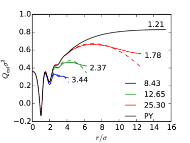
Figure 4: Estimates of $Q(0)$ using the radial distribution function integral (Eq. 30) from different simulation sizes. The value at the origin is the ideal gas contribution, $\rho=0.36\sigma^{-3}$, while the final estimate must be positive. Dotted lines show the partial integral without the correction of Ref. 7. The inverse of the final values (labeled on the plot) should be compared to Tbl. 1. The PY number is smaller than 1.28 due to the integral cutoff.

Figure 4 shows a running integral of the radial distribution function from several of the simulations. The solid lines use the correction proposed by Krüger et. al.,pkrug13

$$Q_{\text{est}}=\rho+\rho^{2}\int_{0}^{L/2}4\pi r^{2}(g(r)-1)\left(1-(\tfrac{r}{L/2})^{3}\right),$$ (30)

where $L$ is the length of one side of the simulation cell. The dotted lines were not corrected (setting the $1-2r/L$ term to $1$ in Eq. 30). The figure also shows that the PY closure yields a reasonable estimate of the RDF up to $4\sigma$, while the remainder is not possible to judge based on our simulation sizes. The long correlation length of this near-critical point system makes for a challenging test case.

Figure 5: Estimates of $Q(m)$ from the Lennard-Jones system for the same simulations shown in Fig. 4. The $L=25.30\sigma$ line shows artificial damping at large $m$ caused by the smoothing spline FFT method on our fixed 128³ grid. Otherwise, all the lines in (a) overlap one another. In (b), only the smallest three $k$-points from each simulation are shown, and the horizontal axis is scaled to show $(2\pi m)^{2}$, anticipating the role of the correlation length (Eq. 20). The dotted line plots Eq. 31 plus a constant using $\eta=1$.

Fig. 5a plots the structure factor, $Q$, using spectroscopy units, $k=2\pi m$. It should be compared with Figs. 3 and 4 of Ref. 29, where the relationship is $\rho^{2}\tilde{h}(k)=Q(k/2\pi)-\rho$. That reference shows the shape of $Q(m)$ near $m=0$ was very flat, and easy to extrapolate. The present case is much more difficult because it is near the critical point and a very large peak has appeared near $m=0$.

Fig. 5b shows the inverse of Fig. 5a near the origin. It is the analogue of Fig. 2 for the lattice gas. For clarity, only the first three points with smallest $m$ from each simulation are shown. These particular $m$-points correspond to averages over plane wave shaped density fluctuations oriented along faces, edges, and corners of the cubic unit cell. All five of the canonical simulation points shown at $m=0$ are extrapolations from these points. Their numerical values are in Table 1.

Fig. 5b also shows two other important points. First, $Q(m)$ computed from the largest simulation size is artificially noisy and scaled downward at high wavenumbers. The scale artifact is due to the inaccuracy of B-spline smoothing past $K_{\text{max}}/2$, where $K_{\text{max}}=128/L$ is set by our numerical grid, which contained 128³ points for every $L$. A similar artifact also appears for the $L=12.65$ simulation just past the right boundary of Fig. 5b. The noise is caused by the discrete nature of the 128³ grid points, which appear at irregularly spaced distances from the origin. It could be eliminated by resamping the data to uniform intervals in $|m|$.

Second, the long-range portion of the LJ potential can be Fourier-transformed according to Ref. 10 to give,

$$c_{\text{LR}}(x=m/\eta)=\frac{4\epsilon}{3}\left[(1-2x^{2})e^{-x^{2}}+2x^{3}\sqrt{\pi}\operatorname{erfc}(x)\right],$$ (31)

where $\eta$ is an inverse distance corresponding to a division between short-range and long-range forces. Recognizing that this term makes an additive contribution to Eq. 15 can accelerate the convergence of the fit in Eq. 16. Indeed, we find that subtracting this term from $Q^{-1}$ makes the first few points much more linear. The result can be visualized from Fig. 5b as the distance between the red and black lines. However, to keep our discussion simple, we have not included it in our estimates.

Similar to the antiferromagnetic lattice gas in Fig. 3a, the estimates of $Q(0)$ are larger than the grand-canonical value, and decrease with increasing cell size. The former figure showed that the extrapolated points, $Q(0)$, quickly converged to second differences of the Helmholtz free energy (Eq. 17). We cannot test this numerically here, since the MD estimates of $\beta\mu^{\text{ex}}$ at finite volumes have uncertainties on the order of the volume.

Instead, we have tested the finite-size corrections to $\beta\mu^{\text{ex}}$ in Eq. 22. Using the value of $Q^{-1}$ and its derivative from Table 1 gives $\Delta\beta\mu^{\text{ex}}=4.18\sigma^{3}/V$. This is a good fit to the size-dependence of $\mu^{\text{ex}}$ seen in simulations. In the limit as $m\to 0$, the finite-size corrections to $Q$ and to $\beta\mu^{\text{ex}}$ are related by a density derivative. Computing the finite-size correction to $Q(0)$ from Eq. 21 gives $\lim_{m\to 0}\Delta Q(m)=-20/V$, which agrees with the density derivative of Eq. 22. The simulation points do not allow a single estimation of the slope near $m=0$ for the largest simulations, but the slope of the $c_{0}$ values vs. $1/V$ appears to be +200 rather than -20 for simulations at intermediate cell-sizes.

Figure 6: Contour plot of the $1/V$ coefficient in the finite-size correction to the free energy, $\partial(\kappa-\beta/\rho)/\partial\rho/2\kappa$ (Eq. 23) as calculated using the MBWR equation of state. Contours are shown every 2$\sigma^{3}$, while variations above $\pm 10\sigma^{3}$ were colored at the max/min values. The axes are LJ temperature and density. Values in the liquid-vapor coexistence region (bottom, under the saturation curve) have been set to zero for clarity.

Because finite size corrections are relatively more important for canonical than grand-canonical simulations, we have plotted the finite size correction to the free energy predicted by the MBWR equation of state in Fig. 6. The result reassures us that the chemical potential calculated by test particle insertion has negligible volume dependence in both gas and liquid states.Near the solidification line, test particle insertion should be expected to slightly overestimate the excess chemical potential, while we get an underestimation for high-temperature liquids near the critical point.

V Conclusions

Kirkwood-Buff integrals are notoriously difficult to calculate from canonical, closed simulations. We have shown that this problem can be helpfully mapped onto the problem of estimating the direct correlation function of Ornstein-Zernike theory in a canonical ensemble. All earlier work used truncated real-space estimates, for which the process of extrapolating to infinite truncation radius, $R$, is ill-posed.nmatu96 ; pgang13 Our exact theory for the canonical ensemble uses the entire simulation volume at once, is manifestly invariant to shifts of the radial distribution function by a constant, and replaces the problem of extrapolating to infinite $R$ with the well-posed problem of extrapolating to zero $m$ within a finite simulation volume.

The density-dependence of the radial distribution function becomes important when estimating the thermodynamic limit.jlebo67 ; jsala96 These higher-order derivatives are very difficult to estimate accurately from simulation data, and it is simpler to test for finite size effects by scaling up the system.pkrug13 This work showed that the principle difficulty in reaching the thermodynamic limit is the size-dependence of the canonical ensemble itself. We then provided a simple, general formula for estimating finite-size corrections of the excess chemical potential from KB coefficients. These corrections are small for the LJ fluid.

Our data in Fig. 5 show excellent agreement for the entire correlation function at low wave-vectors in reciprocal space. Higher wave-vectors require smaller grid-spacing to avoid numerical artifacts, though. Fits using Eq. 16 provide an estimation of both the KB coefficient and the correlation length which are more accurate than radial-distribution function integrals and fit well into the context of integral theories of solution. We have shown that the theory is robust by treating difficult cases with long-range correlations. These can be identified in simulation work from the shape of $Q(m)$ near $m=0$.

We have shown that the zero-frequency limit of the canonical KB theory gives second derivatives of the Helmholtz free energy for simulation sizes larger than about 5 times the correlation length. Further, this theory has several nice properties. In the low density limit, the direct correlation function can be predicted from the long-range form of the interaction energy function. This leads to even better extrapolation to zero frequency. Further information on the applicability of this process is given in the supplementary material. Alternatively, the direct correlation function can be computed from simulation data and used to test common assumptions for OZ closure relations.pdt6 A companion paper uses this process to compute the spatial dielectric response of water.droge18a This use of $Q$ to estimate pair interaction energies was first proposed by Madden and Rice wmadd80 .

Supplementary Material

The supplementary material includes derivations and extended discussion of several formulas from the main text. It provides a definition of the finite-volume radial distribution, free from cutoffs, and consistent with Eq. 2. It also provides explicit expressions for the other derived quantities of Kirkwood-Buff theory in terms of the matrix $Q_{\alpha\gamma}(0|\mu)$. It derives the ensemble correction to the free energy (Eq. 22). Then it gives computable expressions for the correlation function of the finite-size Ising model and an approximate expression for the correlation length of the Lennard-Jones fluid. Both correlation lengths are plotted as a function of state point. Those results provide additional intuitive insight on the long-range correction proposed above.

I Ensemble Dependence

Explicit expressions for the radial distribution functions help to show how ensemble dependence arises in the KB integral. Eq. 1 of the main text can be written as an average over canonical simulations,

$$\left\langle{\hat{\rho}_{\alpha}(r)\hat{\rho}_{\gamma}(0)|\mu,L}\right\rangle =\sum_{n}P(n|\mu,L)\left\langle{\hat{\rho}_{\alpha}(r)\hat{\rho}_{\gamma}(0)|n,L}\right\rangle$$

$$\left\langle{\hat{\rho}_{\alpha}(r)\hat{\rho}_{\gamma}(0)|n,L}\right\rangle =\frac{n_{\gamma}}{V}\sum_{j=1}^{n_{\alpha}}P(r_{\alpha,j}=r|r_{\gamma,1}=0,n,L)$$ (S1)

The conditional probability in the last line gives the probability that the $j^{\text{th}}$ molecule of type $\alpha$ has its center of mass at $r$ given that the first molecule of type $\gamma$ is centered at the origin. When $\alpha=\gamma$, this has the effect of decomposing the sum over $j$ into $j=1$, where we know $r_{j}$ is already at the origin, and $j\neq 1$, where $j$ is distinct from the molecule at the origin. This gives a delta function at the origin plus $n_{\alpha}-1$ times the pair distribution function for fixed $n$. Explicitly,

$$P(r=r_{\alpha,j}|r_{\gamma,1}=0,n,L)=\begin{cases}\delta(r),&\alpha=\gamma,j=1\\ g_{\alpha\gamma}(r|n,L)/V,&\text{o.w.}\end{cases}$$ (S2)

and

$$\left\langle{\hat{\rho}_{\alpha}(r)\hat{\rho}_{\gamma}(0)|n,L}\right\rangle=\frac{n_{\gamma}}{V}\left(\frac{n_{\alpha}-\delta_{\alpha\gamma}}{V}g_{\alpha\gamma}(r|n,L)+\delta_{\alpha\gamma}\delta(r)\right)$$ (S3)

The identification of $g(r|n,L)$ in Eq. S3 agrees with its method of computation from canonical ensemble simulation data by estimating the conditional probability, $P(r=r_{\alpha,j}|r_{\gamma,1}=0,n,L)$. Of course, when the two particles are independent, the conditional probability is $1/V$, and $g(r|n,L)$ is 1. However, even for real molecules with excluded volume, $g(r|n,L)$ always integrates to the volume, $V$. This makes the integral of $g(r|n,L)$ uninformative for number fluctuations – since there are none in a canonical simulation. Explicitly, if we insert Eqns. S3 and S1 into Eq. 1 and integrate, then the $g(r|n,L)$ term drops out and the entire Kirkwood-Buff integral is due to the ensemble correction.

For completeness, we re-state the derived quantities of Kirkwood-Buff theory in terms of the $\nu\times\nu$ matrix ${\bf Q}=[Q_{\alpha\gamma}(0|\mu,L)]$ and using the vector of $\nu$ densities, $\rho$, below.

$$\kappa/\beta =1/\rho^{T}{\bf Q}^{-1}\rho$$ (S4)

$$\bar{V} =\frac{\kappa}{\beta}{\bf Q}^{-1}\rho$$ (S5)

$$\beta V\left[\frac{\partial{\mu_{\alpha}}}{\partial{n_{\gamma}}}\right]_{n,P,T} ={\bf Q}^{-1}-\frac{\beta}{\kappa}\bar{V}\bar{V}^{T}$$ (S6)

$$\left[\frac{\partial{\Pi}}{\partial{\rho_{\alpha}}}\right]_{\mu_{1},\rho_{\gamma\neq 1},T} ={\bf Q_{2}}^{-1}\rho_{2}$$ (S7)

These formulas express the isothermal compressibility, vector of partial molar volumes, matrix of constant-pressure chemical potential derivatives, and vector of $\nu-1$ osmotic pressure derivatives (respectively). The derivative of the osmotic pressure requires a special notation, ${\bf Q_{2}}$, for the $\nu-1\times\nu-1$ sub-matrix of ${\bf Q}$ discarding the first row and column, and a similar notation, $\rho_{2}$ for the $\nu-1$ component vector of solute densities. Note that the entries are discarded from $\bf Q$ before inverting. The equation for $\partial\mu/\partial\rho$ at constant temperature and pressure requires using the relation $dn_{1}\bar{V}_{1}+dn_{2}\bar{V}_{2}=0$ for a constant pressure variation of $n_{1}$ at constant (arbitrary) volume, which does not generalize beyond 2-components.

II Ensemble Correction for the Excess Chemical Potential

The exponent of the excess chemical potential can be written in the grand-canonical ensemble as,

$$e^{-\beta\mu^{\text{ex}}_{\alpha}}=e^{\beta(\mu^{\text{id}}_{\alpha}-\mu_{\alpha})}\equiv Z,$$ (S8)

which we call $Z$ for compactness. The ensemble correction for $Z$ requires alternating derivatives,[15]

$$Z(\mu)=Z(n)+\frac{V}{2V}\sum_{\gamma}\frac{\partial{}}{\partial{(\beta\mu_{\gamma})}}\frac{\partial{}}{\partial{n_{\gamma}}}Z(\mu),$$ (S9)

evaluating the first at constant chemical potentials ($\mu_{\alpha}$) and the second at constant densities ($\mu_{\alpha}^{\text{id}}$). The volume is constant in both, and can be used to transform $n_{\gamma}/V=\rho_{\gamma}$. The first derivative is,

$$\frac{\partial{}}{\partial{\rho_{\gamma}}}Z(\mu)=Z(\mu)\left(\frac{\partial{\beta\mu^{\text{id}}_{\alpha}}}{\partial{\rho_{\gamma}}}-Q^{-1}_{\alpha\gamma}(0)\right).$$ (S10)

The next step requires the other derivative,

$$\frac{\partial{}}{\partial{(\beta\mu_{\gamma})}}Z(\mu)=Z(\mu)\left(\frac{\partial{\beta\mu^{\text{id}}_{\alpha}}}{\partial{\rho_{\alpha}}}Q_{\alpha\gamma}(0)-\delta_{\alpha\gamma}\right),$$ (S11)

which uses the fact that $\mu^{\text{id}}_{\alpha}$ does not depend on any densities other than $\rho_{\alpha}$. Using these in Eq. S9 yields, (to order $1/V$)

$$\frac{Z(\mu)}{Z(n)}=1+\frac{1}{2V}\left(-2\frac{\partial{\beta\mu^{\text{id}}_{\alpha}}}{\partial{\rho_{\alpha}}}+Q_{\alpha\alpha}(0)\left[\left(\frac{\partial{\beta\mu^{\text{id}}_{\alpha}}}{\partial{\rho_{\alpha}}}\right)^{2}+\frac{\partial{{}^{2}\beta\mu^{\text{id}}_{\alpha}}}{\partial{\rho_{\alpha}^{2}}}\right]+Q^{-1}_{\alpha\alpha}(0)-\sum_{\gamma}\frac{\partial{Q^{-1}_{\alpha\gamma}}}{\partial{(\beta\mu_{\gamma})}}\right).$$ (S12)

Since $\partial\beta\mu^{\text{id}}_{\alpha}/\partial\rho_{\alpha}=1/\rho_{\alpha}$, the $Q_{\alpha\alpha}(0)$ term cancels. The final ensemble correction given in the main text is the first term in the expansion of $-\ln Z(\mu)/Z(n)$. Since $Q^{-1}$ is naturally a function of $\rho$, while its derivative in Eq. S12 is taken at constant $\rho$, it is useful to change the independent variables from $\mu$ to $\rho$,

$$\frac{\partial{Q^{-1}_{\alpha\gamma}}}{\partial{(\beta\mu_{\gamma})}}=\sum_{\delta}Q_{\gamma\delta}(0)\frac{\partial{Q^{-1}_{\alpha\gamma}}}{\partial{\rho_{\delta}}}.$$ (S13)

Another alternate formula is,

$$\frac{\partial{Q^{-1}_{\alpha\gamma}}}{\partial{(\beta\mu_{\gamma})}}=-\sum_{ij}Q^{-1}_{\alpha i}\frac{\partial{Q_{ij}}}{\partial{(\beta\mu_{\gamma})}}Q^{-1}_{j\gamma}.$$ (S14)

III Ising Model Distribution Function

The lattice gas in the main text has potential energy function,

$$\beta H(\hat{\rho}|L)=-x\sum_{j=1}^{L}\hat{\rho}_{j-1}\hat{\rho}_{j},$$ (S15)

where we have defined $\beta J\equiv x$ and used periodic boundary conditions, $\hat{\rho}_{L}=\hat{\rho}_{0}$. To compute powers of the transfer matrix,

$$T\equiv\begin{bmatrix}e^{\phi+x}&e^{\phi/2}\\ e^{\phi/2}&1\end{bmatrix},$$ (S16)

we write it as $T=\alpha I+r_{x}\sigma_{x}+r_{z}\sigma_{z}$, where $\sigma_{x}$ and $\sigma_{z}$ are $2\times 2$ Pauli spin matrices and

$$\alpha\equiv(e^{\phi+x}+1)/2,\quad r\equiv[e^{\phi/2},0,(e^{\phi+x}-1)/2]^{T}.$$ (S17)

We also define the scale parameter,

$$y\equiv\frac{\alpha-|r|}{\alpha+|r|}.$$ (S18)

The partition function can then be written as,

$$Z(\phi,L) =\operatorname{Tr}\left[T^{L}\right]=(\alpha+|r|)^{L}(1+y^{L})$$

$$\frac{T^{m}}{(\alpha+|r|)^{m}/2} =(1+y^{m})I+(1-y^{m})(r_{x}\sigma_{x}+r_{z}\sigma_{z})/|r|,$$ (S19)

and it is easy to find expectation values of $$\hat{\sigma}_{z}(j)$$,

$$\left\langle{\hat{\sigma}_{z}(0)}\right\rangle =\operatorname{Tr}\left[T^{L}\sigma_{z}\right]/Z=\left(\frac{1-y^{L}}{1+y^{L}}\right)\frac{r_{z}}{|r|}$$ (S20)

$$\left\langle{\hat{\sigma}_{z}(0)\hat{\sigma}_{z}(j)}\right\rangle =\operatorname{Tr}\left[T^{L-j}\sigma_{z}T^{j}\sigma_{z}\right]/Z$$

$$=\frac{r_{z}^{2}}{|r|^{2}}+\frac{r_{x}^{2}}{|r|^{2}}\frac{y^{j}+y^{L-j}}{1+y^{L}}.$$ (S21)

These can be transformed into average densities and radial distribution functions by substituting, $\hat{\sigma}_{z}(j)=2\hat{\rho}(j)-I$.

Figure S1: Scale of the cosine term in Eq. 18 compared with the correlation length, $L_{c}$, and the interaction energy, $y/\rho(1-\rho)\sim x$ as $x\to 0$. Points mark the scale observed in closed simulations from $L=10$ to $L=512$. The largest $L$ values approach the line most closely.

Fig. S1 shows the prefactor of the cosine-term in $Q^{-1}(m)$, $2y/(1-y^{2})$. Since the prefactor dictates the correlation length estimated by Eq. 16 of the main text, it is important to compare to the analytical $L_{c}$ in this model. In the high temperature limit, $|x|\to 0$, and the prefactor simplifies to $2x\rho(1-\rho)$. At large coupling, the prefactor approaches the analytical correlation length, $L_{c}$. Both limits are shown in the figure.

The finite-size effect on $L_{c}$ was calculated by estimating the prefactor for canonical, closed systems. This estimation is very nearly exact, since $Q^{-1}$ for closed systems maintains its cosine shape, even at high coupling. Those estimates are shown by crosses in the figure. All these estimates show a larger effective correlation at finite sizes. Our simulation lengths were spaced logarithmically in $L$, so the figure suggests that the prefactor scales linearly with $L/L_{c}$.

IV Correlation Length of the Lennard-Jones System

The main text suggests estimating $Q(m)$ near $m=0$ by subtracting a long-range estimate for the direct correlation function,

$$-\tilde{c}_{LR}(m)=\int e^{-2\pi im\cdot r}u_{LR}(r)dr.$$ (S22)

In a companion paper,[30]we show that this estimate is near quantitative accuracy for ionic systems away from any phase transitions.

To apply this ansatz here, we modify the WCA approximation by using a fictitious reference system. WCA showed that the hard-sphere reference system gets the high-wavenumber behavior of $\tilde{c}(m)$ right. Since $\tilde{c}_{LR}(m)$ is small at high wavenumbers, we simply add it to the hard-sphere solution in the mean spherical approximation (MSA),

$$c_{A}(r)=c_{d}(r;\rho\sigma^{3})-\beta\epsilon u_{LR}(r).$$ (S23)

In variance with the main text, we let $u_{\text{LR}}$ be the long-range part of the WCA potential,

$$u_{LR}(r)=\begin{cases}-1,&r<2^{1/6}\\ 4(r^{-12}-r^{-6}),&r\geq 2^{1/6}\end{cases},$$ (S24)

and $r$ is in units of $\sigma$. The function $c_{d}$ is the cubic polynomial on $[0,d)$ given by the MSA solution of the hard sphere system for a diameter chosen by a consistency condition on $Q(0)$. We then multiply the solution by $e^{-\beta\epsilon u_{0}}$ as described in Ref. [29]to smooth the first peak around $r=d$. The solution has better agreement with $\tilde{c}(m)$ at small wavenumber, but still predicts a first peak that is lower than simulation (and lower than the PY solution used in the main text).

However, it is a good approximation for predicting the correlation length. It can be found from Eq. 20 in the main text, using

$$1-\rho c_{0} \equiv\rho Q^{-1}(0)=\frac{\beta}{\rho\kappa}=1-4\pi\rho\int_{0}^{\infty}r^{2}c(r)dr$$ (S25)

$$=\frac{(2\eta+1)^{2}}{(1-\eta)^{4}}-\tfrac{32}{9}\pi\rho\beta\epsilon\sqrt{2}$$ (S26)

$$\rho c_{2} =\frac{4\pi\rho}{6}\int_{0}^{\infty}r^{4}c(r)dr=\tfrac{48}{35}\pi\rho\beta\epsilon 2^{5/6}-\frac{d^{2}}{(1-\eta)^{4}}\Big{(}$$ (S27)

$$\quad(2\eta+1)^{2}(\tfrac{\eta}{20}-\tfrac{3}{16})+3(\eta+\tfrac{1}{8})/2\Big{)}.$$ (S28)

The second part in Eq. S26 is the zeroth-order perturbation, $\int u_{LR}(r)dr$, which matches the corresponding term in the WCA perturbation energy.[29]

Figure S2: Correlation length of the LJ system predicted from LR perturbation, Eqns. S25-S26. The correlation length increases sharply around phase transition points. The model predicts a critical temperature that is too high and a liquid density line that is too dilute.

Fig. S2 plots Eq. S25-S26 for the correlation length along a few isotherms. The numerical value at $\beta^{-1}=1.5\epsilon$ and $\rho=0.36\sigma^{-3}$ is $L_{c}=2\sigma$, which is higher than simulation, but smaller than the PY approximation. The correlation length shows the basic features of the phase diagram, which is remarkable because the hard-sphere system does not have a liquid-vapor transition.

Fig. S2 is based on an approximation to the WCA model, so its phase behavior is only qualitative. The qualitative agreement, however, allows us to conclude that Eq. S22 is a good approximation to the small-wavenumber behavior of $\tilde{c}(m)$ and its inclusion will aid extraction of $\tilde{c}(m)$ from simulation.

It also shows that $L_{c}$ is only few molecular diameters away from phase transitions. This short-ranged behavior translates to a small second derivative of $Q$, which makes estimation of $Q(0)$ possible from the method in the main text without corrections under ordinary circumstances.

References

- (1) John G. Kirkwood and Frank P. Buff. The statistical mechanical theory of solutions. i. J. Chem. Phys., 19(6):774–777, 1951.
- (2) Nobuyuki Matubayasi and Ronald M. Levy. Thermodynamics of the hydration shell. 2. excess volume and compressibility of a hydrophobic solute. J. Phys. Chem., 100(7):2681–2688, 1996.
- (3) Pritam Ganguly and Nico F. A. van der Vegt. Convergence of sampling Kirkwood-Buff integrals of aqueous solutions with molecular dynamics simulations. J. Chem. Theory Comput., 9(3):1347–1355, 2013.
- (4) M. Rovere, D. W. Heermann, and K Binder. The gas-liquid transition of the two-dimensional lennard-jones fluid. J. Phys. Condens. Matter, 2:7009, 1990.
- (5) Sondre K. Schnell, Xin Liu, Jean-Marc Simon, André Bardow, Dick Bedeaux, Thijs J. H. Vlugt, and Signe Kjelstrup. Calculating thermodynamic properties from fluctuations at small scales. J. Phys. Chem. B, 115(37):10911–10918, 2011.
- (6) R. Cortes-Huerto, K. Kremer, and R. Potestio. Communication: Kirkwood-Buff integrals in the thermodynamic limit from small sized molecular dynamics simulations. J. Chem. Phys., 145:141103, 2016.
- (7) Peter Krüger, Sondre K. Schnell, Dick Bedeaux, Signe Kjelstrup, Thijs J. H. Vlugt, and Jean-Marc Simon. Kirkwood-Buff integrals for finite volumes. J. Phys. Chem. Lett., 4(2):235–238, 2013.
- (8) J. J. Salacuse, A. R. Denton, and P. A. Egelstaff. Finite-size effects in molecular dynamics simulations: Static structure factor and compressibility. i. theoretical method. Phys. Rev. E, 53:2382–2390, 1996.
- (9) J. J. Salacuse, A. R. Denton, P. A. Egelstaff, M. Tau, and L. Reatto. Finite-size effects in molecular dynamics simulations: Static structure factor and compressibility. ii. application to a model krypton fluid. Phys. Rev. E, 53(3):2390–2401, 1996.
- (10) U. Essmann, L. Perera, M. L. Berkowitz, T. Darden, H. Lee, and L. G. Pedersen. A smooth particle mesh Ewald method. J. Chem. Phys., 103:8577–8592, 1995.
- (11) David M. Rogers. EwaldCorrel. GitHub, 2017. https://github.com/frobnitzem/EwaldCorrel.
- (12) Peter D. Lax. The Poisson Summation Formula, chapter 30, page 348. Wiley-Interscience, 2002.
- (13) T. L. Beck, M. E. Paulaitis, and L. R. Pratt. The Potential Distribution Theorem and Models of Molecular Solutions, chapter 6, pages 123–141. Cambridge, New York, 2006.
- (14) T. L. Beck, M. E. Paulaitis, and L. R. Pratt. Statistical thermodynamic necessities, chapter 2, pages 23–31. Cambridge, New York, 2006.
- (15) J. L. Lebowitz, J. K. Percus, and L. Verlet. Ensemble dependence of fluctuations with application to machine computations. Phys. Rev., 153(1):250–254, Jan 1967.
- (16) H. Ted Davis. Statistical Mechanics of Phases, chapter 9, pages 442–448. VCH Publishers, New York, 1996.
- (17) J. I. Siepmann, I. R. McDonald, and D. Frenkel. Finite-size corrections to the chemical potential. J. Phys. Cond. Matter, 4(3):679–691, 1992.
- (18) Sacha Friedli and Yvan Velenik. The Ising Model, chapter 3, pages 97–183. Cambridge University Press, Cambridge, UK, 2017.
- (19) J. Reinhard, W. Dieterich, P. Maass, and H. L. Frisch. Density correlations in lattice gases in contact with a confining wall. Phys. Rev. E, 61(1):422–428, 2000.
- (20) C. Borzi, G. Ord, and J. K. Percus. The direct correlation function of a one-dimensional Ising model. J. Stat. Phys., 46(1–2):51–66, 1987.
- (21) Carlos F Tejero. One-dimensional inhomogeneous Ising model: A new approach. J. Stat. Phys., 48(3):531–538, 1987.
- (22) H. Ted Davis. Statistical Mechanics of Phases, chapter 3, pages 128–130. VCH Publishers, New York, 1996.
- (23) Juraj Vavro. Exact solution for the lattice gas model in one dimension. Phys. Rev. E, 63:057104, 2001.
- (24) Hernan L. Martinez, R. Ravi, and Susan C. Tucker. Characterization of solvent clusters in a supercritical Lennard-Jones fluid. J. Chem. Phys., 104:1067, 1996.
- (25) J. J. Nicolas, K. E. Gubbins, W. B. Streett, and D. J. Tildesley. Equation of state for the Lennard-Jones fluid. Mol. Phys., 37(5):1429–1454, 1979.
- (26) J. Karl Johnson, John A. Zollweg, and Keith E. Gubbin s. The Lennard-Jones equation of state revisited. Molecular Physics, 78(3):591–618, 1993.
- (27) P. H. Fries and G. N. Patey. The solution of the Percus-Yevick approximation for fluids with angle-dependent pair interactions. J. Chem. Phys., 85(12):7307–7311, 1986.
- (28) Marcus G. Martin. MCCCS Towhee: a tool for Monte Carlo molecular simulation. Mol. Sim., 39(14–15):1212–1222, 2013.
- (29) John D. Weeks, David Chandler, and Hans C. Andersen. Role of repulsive forces in determining the equilibrium structure of simple liquids. J. Chem. Phys., 54:5237, 1971.
- (30) David M. Rogers. Fluctuation theory of ionic solvation potentials. 2018. submitted.
- (31) William G. Madden and Stuart A. Rice. The mean spherical approximation and effective pair potentials in liquids. J. Chem. Phys., 72:4208, 1980.