Computational efficiency of symplectic integration schemes: Application to multidimensional disordered Klein-Gordon lattices

Abstract

We implement several symplectic integrators, which are based on two part splitting, for studying the chaotic behavior of one- and two-dimensional disordered Klein-Gordon lattices with many degrees of freedom and investigate their numerical performance. For this purpose, we perform extensive numerical simulations by considering many different initial energy excitations and following the evolution of the created wave packets in the various dynamical regimes exhibited by these models. We compare the efficiency of the considered integrators by checking their ability to correctly reproduce several features of the wave packets propagation, like the characteristics of the created energy distribution and the time evolution of the systems’ maximum Lyapunov exponent estimator. Among the tested integrators the fourth order $ABA864$ scheme BCFLMM13 showed the best performance as it needed the least CPU time for capturing the correct dynamical behavior of all considered cases when a moderate accuracy in conserving the systems’ total energy value was required. Among the higher order schemes used to achieve a better accuracy in the energy conservation, the sixth order scheme $s11ABA82\_6$ exhibited the best performance.

1 Introduction

Disordered dynamical systems try to model heterogeneity appearing in nature due to e.g. impurities, imperfections and defects. Typically, disorder is introduced by giving random, uncorrelated values to one or more parameters of a system. A fundamental phenomenon in disordered systems, which is usually referred as ‘Anderson localization’, is the halting of energy propagation in the presence of sufficiently strong disorder A58 . The appearance and/or the destruction of Anderson localization in linear and nonlinear disordered systems, as well as the properties of energy propagation in such models, have attracted extensive attention in theory, numerical simulations and experiments, especially in recent years S93 ; M98 ; CVHRBSGSA05 ; FFGLMWI05 ; SBFS07 ; LAPSMCS08 ; BJZBHLCS08 ; REFFFZMMI08 ; KKFA08 ; PS08 ; FKS09 ; FKS09b ; GMS09 ; SKKF09 ; VKF09 ; SF10 ; LBKSF10 ; F10 ; B11 ; MAP11 ; MAPS11 ; BLSKF11 ; BLGKSF11 ; KMZD11 ; LBF12 ; MP12 ; JBMCJPPSAB12 ; MP13 ; SGF13 ; ABSD14 ; LIF14 ; SKKF14 ; TSL14 ; MKP16 ; ATS16 ; MYKKPY6 ; ASBF17 ; CPKD17 ; DHKBB17 ; ATS17 .

Studies of disordered versions of two basic, nonlinear Hamiltonian lattice models, namely the Klein-Gordon (KG) oscillator lattice and the discrete nonlinear Schrödinger equation (DNLS), revealed the existence of various dynamical behaviors, the so-called ‘weak’ and ‘strong chaos’ spreading regimes, as well as the ‘selftrapping’ regime and determined the statistical characteristics of energy propagation and chaos in these systems FKS09 ; FKS09b ; SKKF09 ; SKKF14 ; SF10 ; LBKSF10 ; F10 ; BLSKF11 ; BLGKSF11 ; LBF12 ; SGF13 ; LIF14 . One basic outcome of these studies is that energy propagation in disordered lattices is a chaotic process which, in general, results in the destruction of Anderson localization.

Although our understanding of the mechanisms which govern energy spreading in disordered nonlinear lattices has improved significantly over the last decade, many important questions concerning mainly the asymptotic behavior of wave packets and the effect of chaos on that behavior are still open. The numerical investigation of these questions requires the accurate integration of Hamiltonian models with many degrees of freedom (of the order of a few thousands) for very long times and for several different disorder realizations in order to obtain solid and reliable statistical results. This is a very demanding computational task, which will be greatly benefited from the use of efficient integration techniques which could allow the accurate long time integration of multidimensional Hamiltonians in feasible CPU times.

Symplectic integrators (SIs) are numerical techniques explicitly designed for the integration of Hamiltonian systems and nowadays are used widely for this purpose (see for example HLW02 ; MQ02 ; MQ06 ; F06 ; BCM08 and references therein). A basic characteristic of these integrators is that they keep the error of the value of the Hamiltonian, i.e. the usually called ‘energy’, bounded as time increases, in contrast to non-symplectic integrators for which the error increases in time. This feature is of particular interest for the long-time integration of disordered nonlinear lattices, as it guarantees the accurate computation of the asymptotic behavior of such systems. In addition, the fact that SIs can achieve this accuracy for relatively large integration time steps results to the decrease of the required CPU time.

For all these reasons SIs based on splitting the system’s Hamiltonian in distinct, integrable parts have already been used for the integration of the KG and DNLS models FKS09 ; SKKF09 ; SF10 ; LBKSF10 ; BLSKF11 ; LBF12 ; SGF13 ; ABSD14 ; TSL14 ; SGBPE14 ; GMS16 ; ASBF17 . In these studies SIs belonging mainly in the so-called SABA schemes LR01 were used. The numerical integration of the KG system, both in one and two dimensions, proved to be computationally easier as the KG models can be split in two integrable parts (the kinetic and the potential energy), while the efficient integration of the DNLS models requires the splitting of the corresponding Hamiltonian in three integrable parts BLSKF11 ; SGBPE14 ; GMS16 . As a result, using the same computational resources and CPU times one can integrate the KG models for times of one or two orders of magnitude higher than the times achieved for the DNLS systems. For this reason ways to improve the efficiency of the symplectic integration of the DNLS model were investigated in SGBPE14 ; GMS16 where the performance of several SIs based on three part splits, with different orders of accuracy, were studied in detail.

A similar analysis for the KG model is lacking, and it is exactly this gap that the current paper fills. In our study we consider a plethora of SIs of various orders not only for the integration of the Hamilton equations of motion, which govern the evolution of orbits in the system’s phase space, but also for the simultaneous integration of the so-called ‘variational equations’, governing the time evolution of small deviation vectors from the studied orbit. These deviation vectors are needed for characterizing the system’s chaoticity through the computation of a chaos indicator SGL16 , like the maximum Lyapunov Characteristic Exponent (mLCE) BGGS80a ; BGGS80b ; S10 we consider in this work. We note that our investigation includes both the one- and two-dimensional KG models.

The paper is organized as follows: In Sect. 2 we describe the two Hamiltonian models we consider in our study, while in Sect. 3 after a brief introduction of the basic properties of SIs we provide detailed information for the symplectic schemes we include in our investigation. Then, in Sect. 4 we present our numerical results on the performance of the various SIs we implemented. Finally, in Sect. 5 we summarize our findings. In the Appendix the explicit form of several operators needed for the symplectic integration of both the one- and two-dimensional KG models are provided.

2 The Klein-Gordon lattice models

The one-dimensional (1D) KG lattice model of $N$ coupled anharmonic oscillators is described by the Hamiltonian

$$H_{1}(\vec{q},\vec{p})=\sum_{i=1}^{N}\left[\frac{p_{i}^{2}}{2}+\frac{\epsilon_{i}}{2}q_{i}^{2}+\frac{q_{i}^{4}}{4}+\frac{1}{2W}\left(q_{i+1}-q_{i}\right)^{2}\right],$$ (1)

where $\vec{q}=(q_{1},q_{2},\ldots,q_{N})$ and $\vec{p}=(p_{1},p_{2},\ldots,p_{N})$ are respectively the generalized positions (representing displacements of oscillators from their equilibriums) and momenta, $\epsilon_{i}$ are parameters chosen uniformly from the interval $[\frac{1}{2},\frac{3}{2}]$, which determine the on-site potentials, while $W$ denotes the disorder strength. We also consider fixed boundary conditions for this lattice, i.e. $q_{N+1}=0$.

A natural, simple, extension of this model in two dimensions is obtained by attributing a scalar displacement, $q_{i,j}$, to each lattice site of a two-dimensional orthogonal arrangement of $N\times M$ oscillators having $N$ nodes in one direction (related to index $i$) and $M$ nodes in the other (related to index $j$). Then, the corresponding 2D KG Hamiltonian is

$$H_{2}(\vec{q},\vec{p})=\sum_{j=1}^{M}\sum_{i=1}^{N}\left\{\frac{p^{2}_{i,j}}{2}+\frac{\epsilon_{i,j}}{2}q^{2}_{i,j}+\frac{q_{i,j}^{4}}{4}+\frac{1}{2W}\left[(q_{i+1,j}-q_{i,j})^{2}+(q_{i,j+1}-q_{i,j})^{2}\right]\right\},$$ (2)

where $p_{i,j}$ is the generalized conjugate momentum of oscillator $(i,j)$ and $\epsilon_{i,j}$ are again chosen uniformly from the interval $[\frac{1}{2},\frac{3}{2}]$. Again fixed boundary conditions are imposed so that $q_{N+1,j}=q_{i,M+1}=0$ for $i=1,2,\ldots,N$, $j=1,2,\ldots,M$.

The dynamics of Hamiltonian (1) was studied in FKS09 ; SKKF09 ; LBKSF10 ; BLSKF11 ; SGF13 ; ABSD14 ; ASBF17 , while system (2) was considered in LBF12 .

3 Symplectic integration schemes

The equations of motion of a Hamiltonian system $H(\vec{q},\vec{p})$ with $m$ degrees of freedom can be written as ${\frac{d\vec{z}}{dt}=\{\vec{z},H\}=L_{H}\vec{z}}$, where $\vec{z}=(\vec{q},\vec{p})$ and $L_{H}=\{\cdot,H\}$ is a differential operator with $\{\cdot,\cdot\}$ being the Poisson bracket defined by $\{F,G\}=\sum_{i=1}^{m}\left(\frac{\partial F}{\partial q_{i}}\frac{\partial G}{\partial p_{i}}-\frac{\partial F}{\partial p_{i}}\frac{\partial G}{\partial q_{i}}\right)$ for any differentiable functions $F(\vec{z})$ and $G(\vec{z})$. The vector $\vec{z}$ corresponds to a point in the $2m$-dimensional phase space of the system, while its time evolution $\vec{z}(t)$ determines an orbit in that space. Using initial conditions $\vec{z}(t_{0})$ at time $t=t_{0}$ we can formally write the solution $\vec{z}(t_{0}+\tau)$ of the Hamilton equations of motion at time $t=t_{0}+\tau$ as $\vec{z}(t_{0}+\tau)=\sum_{i\geq 0}\frac{\tau^{i}}{i!}L_{H}^{i}\vec{z}(t_{0})=e^{\tau L_{H}}\vec{z}(t_{0})$. So $e^{\tau L_{H}}$ is the operator which propagates in time the coordinate vector $\vec{z}$ by $\tau$ time units. In general, the action of this operator is not known analytically.

In many cases the Hamiltonian function $H(\vec{z})$ can be written as a sum of two integrable parts, $H(\vec{z})=A(\vec{z})+B(\vec{z})$, so that the action of operators $e^{\tau L_{A}}$ and $e^{\tau L_{B}}$ is known analytically. An explicit SI of order $n$, $n\in\mathbb{N}$, approximates the action of operator $e^{\tau L_{H}}$ by a series of products of operators $e^{a_{i}\tau L_{A}}$ and $e^{b_{i}\tau L_{B}}$, i.e.

$$e^{\tau L_{H}}=e^{\tau\left(L_{A}+L_{B}\right)}=\prod_{i=1}^{p}e^{a_{i}\tau L_{A}}e^{b_{i}\tau L_{B}}+\mathcal{O}(\tau^{n+1}),$$ (3)

where $a_{i}$, $b_{i}$, $i=1,2,\ldots,p$, are appropriately chosen constants for obtaining the desired order of accuracy. Usually the total number of applications of the simple operators $e^{a_{i}\tau L_{A}}$ and $e^{b_{i}\tau L_{B}}$ is referred as the number of ‘steps’ of the integrator.

Both the 1D (1) and the 2D (2) KG Hamiltonians, $H_{i}(\vec{q},\vec{p})$, $i=1,2$, can be written as a sum of two integrable parts: the kinetic energy $A_{i}(\vec{p})$, which depends only on the system’s momenta, and the potential energy $B_{i}(\vec{q})$, which is a function of only the generalized positions, i.e. $H_{i}(\vec{q},\vec{p})=A_{i}(\vec{p})+B_{i}(\vec{q})$. Thus, SIs based on two part splitting can be applied straightforwardly for the numerical integration of systems (1) and (2).

Over the years several SIs of various orders and different number of steps have been developed and implemented. SIs of higher order achieve better accuracy for the same integration time step $\tau$, but their implementation could require more computational effort as they contain more steps than low order schemes. In our study we consider in total 33 SIs whose order ranges from 2 up to 8. In the remaining part of this section we briefly present all these SIs.

3.1 Symplectic integrators of order two

The simplest symmetric SI of order two is the so-called ‘leap frog’ integrator ($LF$) or Verlet integrator (see for example R83 and (HLW02, , Sect. I.3.1)), having 3 steps

$$LF(\tau)=e^{a_{1}\tau L_{A}}e^{b_{1}\tau L_{B}}e^{a_{2}\tau L_{A}},$$ (4)

with $a_{1}=a_{2}=\frac{1}{2}$ and $b_{1}=1$. In our study we also consider the second order, 5 step schemes $SABA_{2}$, $SBAB_{2}$ LR01 having respectively the forms

$$SABA_{2}(\tau)=e^{a_{1}\tau L_{A}}e^{b_{1}\tau L_{B}}e^{a_{2}\tau L_{A}}e^{b_{1}\tau L_{B}}e^{a_{1}\tau L_{A}},$$ (5)

with $a_{1}=\frac{1}{2}-\frac{1}{2\sqrt{3}}$, $a_{2}=\frac{1}{\sqrt{3}}$, $b_{1}=\frac{1}{2}$, and

$$SBAB_{2}(\tau)=e^{b_{1}\tau L_{B}}e^{a_{1}\tau L_{A}}e^{b_{2}\tau L_{B}}e^{a_{1}\tau L_{A}}e^{b_{1}\tau L_{B}},$$ (6)

for $a_{1}=\frac{1}{2}$, $b_{1}=\frac{1}{6}$ and $b_{2}=\frac{2}{3}$, as well as the $ABA82$ SI M95 ; FLBCMM13 of 9 steps

$$ABA82(\tau)=e^{a_{1}\tau L_{A}}e^{b_{1}\tau L_{B}}e^{a_{2}\tau L_{A}}e^{b_{2}\tau L_{B}}e^{a_{3}\tau L_{A}}e^{b_{2}\tau L_{B}}e^{a_{2}\tau L_{A}}e^{b_{1}\tau L_{B}}e^{a_{1}\tau L_{A}},$$ (7)

whose coefficients $a_{i}$, $b_{i}$, $i=1,2,3$ can be found in Table 2 of FLBCMM13 . We note that the $ABA82$ integrator is called $SABA_{4}$ in LR01 .

3.2 Symplectic integrators of order four

A way to construct higher order SIs is through a composition (i.e. successive application) of lower order schemes. A composition approach of this kind was proposed in Y90 . According to that method, starting from a SI $S_{2n}(\tau)$ of order $2n$ we construct a SI $S_{2n+2}(\tau)$ of order $2n+2$ as

$$S_{2n+2}(\tau)=S_{2n}(d_{1}\tau)S_{2n}(d_{0}\tau)S_{2n}(d_{1}\tau),$$ (8)

where $d_{0}=-2^{1/(2n+1)}/[2-2^{1/(2n+1)}]$ and $d_{1}=1/[2-2^{1/(2n+1)}]$. We note that if we start from a second order integrator $S_{2}$ then the construction of the SI $S_{2n+2}$ requires the application of $S_{2}$ $3^{n}$ times. Obviously with this approach the number of steps of the $S_{2n+2}$ scheme grows rapidly when $n$ increases, despite the fact that adjacent applications of the same basic operators $e^{a_{i}\tau L_{A}}$, or $e^{b_{i}\tau L_{B}}$ can be grouped together.

Starting from a SI of order two we can apply the composition technique (8) for $n=2$ and create a SI of order four. If the second order SI used is the $LF$ scheme (4) the created SI has 7 steps and was introduced in FR90 ; Y90 . We denote this integrator by $FR4$. Its form is

$$FR4(\tau)=e^{a_{1}\tau L_{A}}e^{b_{1}\tau L_{B}}e^{a_{2}\tau L_{A}}e^{b_{2}\tau L_{B}}e^{a_{2}\tau L_{A}}e^{b_{1}\tau L_{B}}e^{a_{1}\tau L_{A}},$$ (9)

with $a_{1}=\frac{1}{2\left(2-2^{1/3}\right)}$, $a_{2}=\frac{1-2^{1/3}}{2\left(2-2^{1/3}\right)}$, $b_{1}=\frac{1}{2-2^{1/3}}$, $b_{2}=-\frac{2^{1/3}}{2-2^{1/3}}$. Applying the composition (8) to the second order integrators $SABA_{2}$ (5), $SBAB_{2}$ (6) and $ABA82$ (7) we obtain the fourth order schemes $SABA_{2}Y4$, $SBAB_{2}Y4$ and $ABA82Y4$, having 13, 13 and 25 steps respectively.

In LR01 it was shown that if the double Poisson bracket $\{B,\{B,A\}\}$ leads to an expression which can be seen as an integrable Hamiltonian, then the accuracy of the $SABA_{2}$ (5) and the $SBAB_{2}$ (6) integrators can be improved by applying a corrector term $C(\tau)=e^{-\tau^{3}\frac{c}{2}L_{\{B,\{B,A\}\}}}$ before and after the application of the main body of these integrators. We note that $c=\frac{(2-\sqrt{3})}{24}$ for $SABA_{2}$ and $c=\frac{1}{72}$ for $SBAB_{2}$. For the KG Hamiltonians (1) and (2) $\{B,\{B,A\}\}$ depends only on the generalized positions, so it corresponds to an integrable system and the corrector term $C(\tau)$ can be written analytically. Thus, applying this corrector we get two SIs of order four, which we name $SABA_{2}C$ and the $SBAB_{2}C$, having 7 steps each.

In addition, we consider in our analysis the fourth order SIs $ABA864$ and $ABAH864$ introduced in FLBCMM13 ; BCFLMM13 , which have 15 and 17 steps respectively. The values of the coefficients $a_{i}$, $b_{i}$ for the $ABA864$ and $ABAH864$ integrators can be found in Tables 3 and 4 of BCFLMM13 respectively.

3.3 Symplectic integrators of order six

Applying the composition technique (8) with $n=4$ to the fourth order SIs $FR4$, $SABA_{2}Y4$, $SBAB_{2}Y4$, $ABA82Y4$, $SABA_{2}C$ and $ABA864$ we construct the sixth order integrators $FR4Y6$, $SABA_{2}Y4Y6$, $SBAB_{2}Y4Y6$, $ABA82Y4Y6$, $SABA_{2}CY6$ and $ABA864Y6$ having 19, 37, 37, 73, 19 and 43 steps respectively.

In Y90 a composition technique for creating a sixth order SI $S_{6}(\tau)$, starting from a second order SI $S_{2}(\tau)$ was presented. This composition has the form

$$S_{6}(\tau)=S_{2}(w_{3}\tau)S_{2}(w_{2}\tau)S_{2}(w_{1}\tau)S_{2}(w_{0}\tau)S_{2}(w_{1}\tau)S_{2}(w_{2}\tau)S_{2}(w_{3}\tau),$$ (10)

and requires less steps than the successive application of (8) first with $n=2$ and then with $n=4$. In Y90 three different sets of coefficients $w_{i}$, $i=0,1,2,3$ were given. In our study we implement the set described as ‘solution A’ in Table 1 of Y90 because according to M95 it shows the best performance among the composition schemes presented in Y90 . This set corresponds to the composition method named $s7odr6$ in KL97 . Applying the composition scheme (10) to the second order integrators $SABA_{2}$ (5), $SBAB_{2}$ (6) and $ABA82$ (7) we obtain the sixth order schemes $SABA_{2}Y6$, $SBAB_{2}Y6$ and $ABA82Y6$, having 29, 29 and 57 steps respectively.

We also consider the composition scheme named $s9odr6b$ in KL97 , which is based on 9 successive applications of $S_{2}(\tau)$ in order to create a SI of order six

$$s9odr6b(\tau)=S_{2}(\delta_{1}\tau)S_{2}(\delta_{2}\tau)S_{2}(\delta_{3}\tau)S_{2}(\delta_{4}\tau)S_{2}(\delta_{5}\tau)S_{2}(\delta_{4}\tau)S_{2}(\delta_{3}\tau)S_{2}(\delta_{2}\tau)S_{2}(\delta_{1}\tau),$$ (11)

as well as, an 11 stage composition method presented in SS05 , which we call $s11odr6$

$$s11odr6(\tau)=S_{2}(\gamma_{1}\tau)S_{2}(\gamma_{2}\tau)\cdots S_{2}(\gamma_{5}\tau)S_{2}(\gamma_{6}\tau)S_{2}(\gamma_{5}\tau)\cdots S_{2}(\gamma_{2}\tau)S_{2}(\gamma_{1}\tau).$$ (12)

The values of $\delta_{i}$, $i=1,\ldots,5$ of (11) can be found in the appendix of KL97 , while the values $\gamma_{i}$, $i=1,\ldots,6$ of (12) are reported in Section 4.2 of SS05 . Using $SABA_{2}$ (5) as the second order SI $S_{2}$ in (11) and (12) we get two SIs of order six, which we call $s9SABA_{2}6$ and $s11SABA_{2}6$, having 37 and 45 steps respectively, while putting in (11) and (12) the $ABA82$ (7) integrator we get the sixth order SIs $s9ABA82\_6$ and $s11ABA82\_6$, having 73 and 89 steps respectively.

3.4 Symplectic integrators of order eight

Finally we include in our study some SIs of order eight which are based on appropriate compositions of a second order integrator $S_{2}$.

First we consider the composition scheme presented in Y90 , which contains 15 applications of $S_{2}$. In particular, we implement the scheme referred as ‘solution D’ in Table 2 of Y90 because, according to M95 ; SS05 it performs better than the other composition schemes of Y90 . Using as $S_{2}$ in this scheme the $SABA_{2}$ (5) integrator we end up with an eight order SI, which we name $SABA_{2}Y8$, having 61 steps, while the use of $ABA82$ (7) in the place of $S_{2}$ results to the $ABA82Y8$ scheme having 121 steps.

In addition, we consider the composition scheme $s15odr8$ of KL97 having 15 applications of $S_{2}$ and the 19 stage method presented in Section 4.3 of SS05 , which requires 19 applications of $S_{2}$. We call the latter scheme $s19odr8$. Using $SABA_{2}$ (5) in the place of $S_{2}$ for both these techniques we get the eight order SIs $s15SABA_{2}8$ and $s19SABA_{2}8$, having 61 and 77 steps respectively, while the use of the second order SI $ABA82$ (7) gives two integrators of order eight, which we name $s15ABA82\_8$ and $s19ABA82\_8$, having 121 and 153 steps respectively.

4 Numerical results

In order to investigate the performance of the various SIs presented in Sect. 3 we follow the time evolution of different initial excitations of Hamiltonians (1) and (2) by numerically solving their equations of motion. The efficiency of the considered SIs is checked by testing their ability to correctly reproduce several characteristics of the resulting energy propagation. In addition, we quantify the systems’ chaoticity by evaluating the mLCE, which is the most commonly used chaos indicator. For this purpose we use the various SIs to also integrate the systems’ variational equations, which govern, at first order approximation, the time evolution of an infinitesimal perturbation (usually refereed as a deviation vector) from a considered orbit in the systems’ phase space. This vector is needed for the computation of the mLCE $\Lambda$, because $\Lambda$ can be estimated as the limit for $t\rightarrow\infty$ of the quantity

$$L(t)=\frac{1}{t}\ln\left(\frac{\|\vec{w}(t_{0}+t)\|}{\|\vec{w}(t_{0})\|}\right),$$ (13)

often called finite time mLCE, i.e. $\Lambda=\lim_{t\rightarrow\infty}L(t)$ BGGS80a ; BGGS80b ; S10 . In (13) $\vec{w}(t_{0}+t)$ and $\vec{w}(t_{0})$ are deviation vectors from the studied orbit at times $t_{0}$ and $t_{0}+t$ respectively ($t>0$), while $\|\cdot\|$ denotes the usual vector norm. For autonomous Hamiltonian systems like (1) and (2), $L(t)$ converges to a positive value for chaotic orbits, while for regular orbits it tends to zero as $L(t)\propto t^{-1}$ BGS76 ; S10 .

For a Hamiltonian system $H(\vec{z})=H(\vec{q},\vec{p})$ with $m$ degrees of freedom an initial deviation vector $\vec{w}(t_{0})=(\vec{\delta z}(t_{0}))=(\vec{\delta q}(t_{0}),\vec{\delta p}(t_{0}))$ having as coordinates small changes from an orbit’s initial conditions evolves in time according to the variational equations

$$\frac{d\vec{w}(t)}{dt}=\left[\textbf{J}_{2m}\cdot\textbf{D${}^{2}_{H}$}(\vec{z}(t))\right]\cdot\vec{w}(t_{0}),$$ (14)

where $\textbf{J}_{2m}=\left[\begin{array}[]{cc}\textbf{0}_{m}&\textbf{I}_{m}\\ -\textbf{I}_{m}&\textbf{0}_{m}\end{array}\right]$ with $\textbf{I}_{m}$ being the $m\times m$ identity matrix and $\textbf{0}_{m}$ being the $m\times m$ zero matrix, and $\textbf{D${}^{2}_{H}$}(\vec{z}(t))$ is a $2m\times 2m$ matrix with elements $\textbf{D${}^{2}_{H}$}(\vec{z}(t))_{i,j}=\left.\frac{\partial^{2}H}{\partial z_{i}\partial z_{j}}\right|_{\vec{z}(t)}$, $i,j=1,2,\ldots,2m$. Since the elements of $\textbf{D${}^{2}_{H}$}(\vec{z}(t))$ explicitly depend on the system’s orbit, the variational equations (14) have to be integrated together with the Hamilton equations of motion. According to the so-called ‘tangent map method’ SG10 ; GS11 ; GES12 this task can be performed by using symplectic integration schemes which are appropriately extended to integrate both sets of differential equations together. From (3) we see that the dynamics induced by Hamiltonian $H$ can be approximated by successive applications of the dynamics produced by the integrable Hamiltonians $A$ and $B$ through the application of operators $e^{a_{i}\tau L_{A}}$ and $e^{b_{i}\tau L_{B}}$. This decomposition of the dynamics can be extended also to the evolution of deviation vectors through the successive applications of generalized operators which propagate in time both the orbit and the deviation vector under the action of Hamiltonians $A$ and $B$. We denote these operators by $e^{a_{i}\tau L_{AV}}$ and $e^{b_{i}\tau L_{BV}}$. The explicit form of these operators for Hamiltonians (1) and (2) is given in Appendix A.

4.1 One-dimensional KG model

In our numerical simulations we create a disorder realization for the 1D KG model (1) having $N=1000$ sites and we follow the evolution of different initial excitations up to a final integration time $t_{f}=10^{7}$. Previous studies FKS09 ; SKKF09 ; LBKSF10 ; F10 ; BLSKF11 shown that the 1D KG model can exhibit three main dynamical regimes: the weak chaos, strong chaos and selftrapping regimes, depending on the choice of different parameter values and initial excitations. In order to investigate the potential influence of these regimes on the performance of the various SIs we study six different cases of initial excitations for $t_{0}=0$. In particular, we consider the following cases.
Case A: we perform a single site excitation of a site at the middle of the lattice for $W=4$ and total energy $H_{1A}=0.4$.
Case B: we initially excite $N_{I}=37$ adjacent sites at the middle of the lattice for $W=3$ and total energy $H_{1B}=0.37$, so that the energy per initially exited particle is $H_{1B}/N_{I}=0.01$.
Case C: initial excitation of $N_{I}=21$ central sites for $W=4$ and total energy $H_{1C}=4.2$ (energy per initially exited particle $H_{1C}/N_{I}=0.2$).
Case D: excitation of a single, central site for $W=4$ and total energy $H_{1D}=1.5$.
Case E: initial excitation of $N_{I}=100$ central sites for $W=4$ and total energy $H_{1E}=1$.
Case F: all sites are initially excited for $W=4$ and total energy $H_{1F}=10$.
We note that in cases of multiple site initial excitations the same amount of energy is given to each excited site as kinetic energy. This is done by choosing the same, appropriate value for the momentum of the initially excited sites, having a random sign for each site, while all other momenta and positions are set to zero.

For each case we consider normalized energy distributions

$$E_{i}=\left[\frac{p_{i}^{2}}{2}+\frac{\epsilon_{i}q_{i}^{2}}{2}+\frac{q_{i}^{4}}{4}+\frac{(q_{i+1}-q_{i})^{2}}{4W}\right]/H_{1}\,,\,\,\,i=1,2,\ldots,N,$$ (15)

and evaluate their second moment $m_{2}=\sum_{i=1}^{N}(i-\bar{i})^{2}E_{i}$ and participation number $P=1/\sum_{i=1}^{N}E_{i}^{2}$, with $\bar{i}=\sum_{i=1}^{N}iE_{i}$. The efficiency of each SI is evaluated by checking its ability to correctly reproduce the dynamics of the energy propagation. For this reason we look at the shape of the computed energy profiles, as well as at the time evolution of $m_{2}(t)$, $P(t)$ and $L(t)$. For the computation of the mLCE we consider in each studied case a random initial deviation vector having nonzero coordinates only for the initially excited sites. In addition we quantify the accuracy of our computations by registering the time evolution of the absolute relative energy error $E_{r}(t)=\left|\right[H_{1}(t)-H_{1}(t_{0}=0)\left]/H_{1}(t_{0}=0)\right|$.

Cases A and B belong to the weak chaos regime, case C to the strong chaos regime, while case D is a representative case of the selftrapping behavior. For all these cases the energy does not reach the lattice’s boundaries up to the final integration time $t_{f}$ of our simulations, because we want to mimic energy propagation in an infinite lattice. Cases E and F correspond to extended initial excitations, which can reach the fixed boundaries of the lattice during our simulations. We considered these two cases in order to test the performance of the integration schemes also for some general excitations where the majority or even all sites eventually become excited.

The 33 considered SIs in our study have different orders and various numbers of steps. In order to compare their efficiency in correctly capturing the dynamics of system (1) we adjust the integration time step $\tau$ of each scheme to achieve practically the same level of accuracy. A typically acceptable level of accuracy in numerical investigations of multidimensional disordered systems correspond to values $E_{r}\lesssim 10^{-4}$ FKS09 ; SKKF09 ; LBKSF10 ; F10 ; BLSKF11 . Trying to improve a bit this accuracy we report in Table 1 the values of $\tau$ which set the obtained energy accuracy at $E_{r}\approx 10^{-5}$.

Table 1: Information on the performance of several SIs of order $n$ used for the integration of the equations of motion and the variational equations of the 1D KG model (1) up to final time $t_{f}=10^{7}$ for the initial excitation of case B (see text for more details). The number of steps of each SI is given along with the integration time step $\tau$ used for obtaining an absolute relative energy error $E_{r}\approx 10^{-5}$. The required CPU time in seconds $T_{C}$ needed for each integrator is also reported. All simulations were performed on an Intel Xeon E5-2623 with 3.00 GHz.

SI $n$ Steps $\tau$ $T_{C}$ SI $n$ Steps $\tau$ $T_{C}$ $ABA82$ 2 9 0.04 8528 $SABA_{2}Y6$ 6 29 0.55 1402 $SABA_{2}$ 2 5 0.02 12779 $s9SABA_{2}6$ 6 37 0.67 1406 $SBAB_{2}$ 2 5 0.02 14431 $ABA864Y6$ 6 43 0.65 1652 $LF$ 2 3 0.01 32280 $SBAB_{2}Y6$ 6 29 0.46 1747 $ABA864$ 4 15 0.56 840 $s9ABA82\_6$ 6 73 0.93 1920 $ABAH864$ 4 17 0.38 1349 $FR4Y6$ 6 19 0.18 3090 $ABA82Y4$ 4 25 0.26 2629 $SABA_{2}CY6$ 6 19 0.37 3238 $SABA_{2}C$ 4 7 0.19 3351 $SABA_{2}Y4Y6$ 6 37 0.28 3366 $SABA_{2}Y4$ 4 13 0.12 3560 $SBAB_{2}Y4Y6$ 6 37 0.28 3846 $FR4$ 4 7 0.09 3310 $SABA_{2}Y8$ 8 61 0.20 7294 $SBAB_{2}Y4$ 4 13 0.12 3835 $ABA82Y8$ 8 121 0.22 12474 $SBAB_{2}C$ 4 7 0.14 4778

In Fig. 1 we see results obtained for four integrators of Table 1, namely $ABA82$ (blue curves), $ABA864$ (red curves), $SABA_{2}Y6$ (green curves) and $SABA_{2}Y8$ (brown curves) for case B. The values of used $\tau$ for each integrator results in keeping the absolute relative energy error bounded at the level of $E_{r}\approx 10^{-5}$ [Fig. 1(a)]. All integrators reproduce correctly the dynamical evolution of the system as the produced results for $m_{2}(t)$ [upper curves of Fig. 1(b)] and $P(t)$ [lower curves of Fig. 1(b)], as well as the normalized energy profiles $E_{i}$ at $t_{f}=10^{7}$ [Fig. 1(c)] practically overlap. It is worth noting that the results of Fig. 1(c) show that the second moment and the participation number of the produced wave packet eventually grow as $m_{2}(t)\propto t^{1/3}$ and $P(t)\propto t^{1/6}$ respectively, in accordance to previously published works FKS09 ; SKKF09 ; LBKSF10 ; BLSKF11 . In Fig. 1(d) we show the required CPU time $T_{C}$ needed by each SI for this simulation. From this figure it becomes obvious that the $ABA864$ scheme has the best performance as it requires the least CPU time.

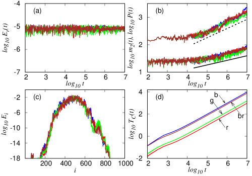
Figure 1: Results for the integration of case B of Hamiltonian (1) by the SIs $ABA82$ of order two, $ABA864$ of order four, $SABA_{2}Y6$ of order six and $SABA_{2}Y8$ of order eight [(b) blue; (r) red; (g) green; (br) brown]: (a) the time evolution of the absolute relative energy error $E_{r}(t)$, (b) the time evolution of the second moment $m_{2}(t)$ (upper curves) and participation number $P(t)$ (lower curves), (c) the logarithm of the normalized energy distribution $E_{i}$ at time $t_{f}=10^{7}$ as a function of lattice site index $i$, and (d) the time evolution of the required CPU time $T_{C}(t)$ in seconds. The straight lines in (b) guide the eye for slopes $1/3$ (dashed line) and $1/6$ (solid line). Panels (a), (b) and (d) are in $\log-\log$ scale. In panels (a), (b) and (c) the four different curves practically overlap each other.

In Fig. 1 we presented results for the best performing integrators for each order reported in Table 1. We note that although the results of Table 1 and Fig. 1 were obtained for the excitation of case B, the SIs have similar behaviors for all the other studied cases.

From the results of Table 1 we see that the SIs exhibiting the best performance (in descending order of efficiency) are: the fourth order schemes $ABA864$, $ABAH864$ and the sixth order schemes $SABA_{2}Y6$, $s9SABA_{2}6$, $ABA864Y6$. In Fig. 2 we present results based on the numerical solution of the variational equations of Hamiltonian (1) which are obtained by these five integrators for the weak chaos case B [Figs. 2(a) and (b)], as well as the extended excitation of case E [Figs. 2(c) and (d)]. From Figs. 2(a) and (c) we see that the time evolution of the finite time mLCE $L(t)$ (13) is qualitative the same for all these SIs. We note that in the weak chaos case B [Fig. 2(a)] the $L(t)$ eventually tends to decrease in a way which is very similar to the law $L(t)\propto t^{-1/4}$ reported in SGF13 . This law is different than the $L(t)\propto t^{-1}$ behavior seen for regular orbits, denoting that the strength of chaoticity decreases as the wave packet spreads without showing any sign of crossover to regular dynamics SGF13 . On the other hand, for the fully chaotic case E where all sites are initially excited $L(t)$ shows the typical behavior of chaos as it saturates quite fast to a constant positive value [Fig. 2(c)]. The similarities of Figs. 2(b) and (d) clearly show that the performance of the integration schemes does not depend on the system’s initial conditions and dynamical regime.

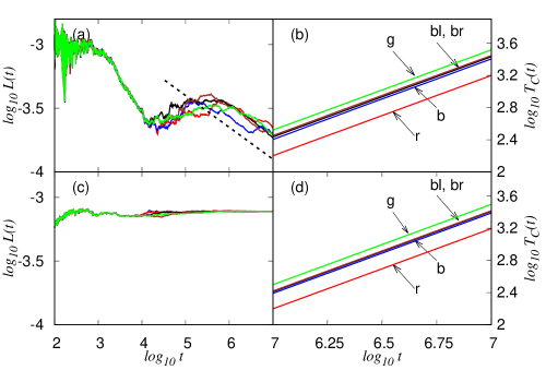
Figure 2: Results obtained by the integration of the variational equations of Hamiltonian (1) for cases B [panels (a), (b)] and E [panels (c), (d)] through the application of the SIs $ABA864$, $ABAH864$, $SABA_{2}Y6$, $s9SABA_{2}6$, $ABA864Y6$ [(r) red; (b) blue; (bl) black; (br) brown; (g) green]: the time evolution of $L(t)$ (13) [(a) and (c)], and of the required CPU time $T_{C}(t)$ [(b) and (d)]. All panels are in $\log-\log$ scale. The straight dashed line in (a) guides the eye for slope $-1/4$. The curves in (c) practically overlap, as well as the curves for $SABA_{2}Y6$, $s9SABA_{2}6$ in (b) and (d).

In Table 1 only 23 SIs of the 33 considered schemes are reported because the remaining 10 SIs ($ABA82Y4Y6$, $ABA82Y6$, $s11SABA_{2}6$, $s11ABA82\_6$ of order six and $SABA_{2}Y8$, $ABA82Y8$, $s15SABA_{2}8$, $s19SABA_{2}8$, $s15ABA82\_8$, $s19ABA82\_8$ of order eight) are unstable. This means that in order to get $E_{r}\approx 10^{-5}$ they require a rather large integration time step $\tau$, which is not appropriate for them because they fail to keep the values of $E_{r}(t)$ bounded. Requiring a lower bounding value for $E_{r}$, e.g. $E_{r}\approx 10^{-8}$ (which might not be necessarily needed in general investigations of disordered lattice dynamics), leads to smaller values of $\tau$ for which also these integrators keep the $E_{r}$ values bounded. We note here that all SIs listed in Table 1 can achieve $E_{r}\approx 10^{-8}$ by appropriately lowering their integration time step.

By performing a similar analysis to the one presented in Figs. 1 and 2 for $E_{r}\approx 10^{-8}$ we find that the five best performing SIs (in descending order) are $s11ABA82\_6$ of order six, $s15ABA82\_8$, $s19ABA82\_8$ of order eight and $SABA_{2}Y6$, $s9ABA82\_6$ of order six. In Fig. 3 we present results obtained by these five schemes for case B. From Fig. 3(a) we see that the integration time step $\tau$ for each integrator was chosen so that $E_{r}\approx 10^{-8}$. All integrators succeeded in capturing the correct time evolution of $m_{2}(t)$, $P(t)$ [Fig. 3(b)] and $L(t)$ [Fig. 3(c)] by producing results similar to the ones reported if Fig. 1(b) and Fig. 2(a) respectively. From the results of Fig. 3(d) we see that all five SIs require more CPU time than the best five schemes used to obtain $E_{r}\approx 10^{-5}$ [Fig. 3(b)].

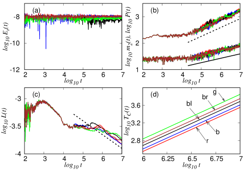
Figure 3: Results for the integration of case B of Hamiltonian (1) by the SIs $s11ABA82\_6$ (order six) for $\tau=0.42$, $s15ABA82\_8$ (order eight) for $\tau=0.48$, $s19ABA82\_8$ (order eight) for $\tau=0.59$, $SABA_{2}Y6$ (order six) for $\tau=0.18$ and $s9ABA82\_6$ (order six) for $\tau=0.50$ [(r) red; (b) blue; (bl) black; (br) brown; (g) green]: the time evolution of the logarithm of (a) $E_{r}(t)$, (b) $m_{2}(t)$ (upper curves) and $P(t)$ (lower curves), (c) $L(t)$ and (d) $T_{C}(t)$. All panels are in $\log-\log$ scale. The straight lines in (b) guide the eye for slopes $1/3$ (dashed line) and $1/6$ (solid line), while in (c) the straight dashed line corresponds to slope $-1/4$.

4.2 Two-dimensional KG model

We also study the performance of the various SIs for the case of the 2D KG model (2). For our simulations we consider a two-dimensional $N\times M$ lattice for $N=M=200$ (note that this corresponds to a Hamiltonian system with 40000 degrees of freedom!), create a disorder realization by attributing some random values to the $\epsilon_{i,j}$ parameters in (2), which remain constant in our numerical experiments, and follow the evolution of energy excitations and deviation vectors up to $t_{f}=10^{6}$.

By solving the system’s equations of motion we keep track of the energy distribution characteristics for three different cases of initial excitations. In particular, we consider the following cases.
Case I: we perform a single site excitation of a site at the center of the lattice for $W=10$ and total energy $H_{2I}=0.3$.
Case II: similar to case I but for $W=10$ and total energy $H_{2II}=2.0$.
Case III: all sites are initially excited, having the same amount of initial energy, for $W=10$ and total energy $H_{2III}=10$.
We note that case I corresponds to the system’s weak chaos regime and case II to the selftrapping regime, while case III represents a general, extended initial excitation. The dynamics of cases I and II was studied in LBF12 .

As in the 1D case we consider two-dimensional normalized energy distributions

$$\begin{array}[]{lll}\displaystyle E_{i,j}&=&\Bigg{\{}\displaystyle\frac{p^{2}_{i,j}}{2}+\frac{\epsilon_{i,j}q^{2}_{i,j}}{2}+\frac{q_{i,j}^{4}}{4}+\frac{1}{4W}\bigg{[}(q_{i+1,j}-q_{i,j})^{2}+(q_{i,j+1}-q_{i,j})^{2}\\ &&\displaystyle+(q_{i,j}-q_{i-1,j})^{2}+(q_{i,j}-q_{i,j-1})^{2}\bigg{]}\Bigg{\}}/H_{2}\,,\,\,\,i=1,\ldots,N,\,\,j=1,\ldots,M,\end{array}$$ (16)

and evaluate their second moment $m_{2}=\sum_{i}^{N}\sum_{j}^{M}\left\|(i,j)-(\bar{i},\bar{j})\right\|^{2}E_{i,j}$ and participation number $P=\left(\sum_{i}^{N}\sum_{j}^{M}E_{i,j}^{2}\right)^{-1}$, with $(\bar{i},\bar{j})=\sum_{i=1}^{N}\sum_{j=1}^{M}(i,j)E_{i,j}$. In addition, by solving the system’s variational equations we follow the time evolution of deviation vectors and compute, to the best of our knowledge for the first time, the finite time mLCE (13) for this model. The initial deviation vector used has random, nonzero coordinates only at a square of $4\times 4=16$ sites at the center of the lattice. Due to the complexity of the set of equations of motion and the variational ones we explicitly present in the Appendix A the form of operators $e^{\tau L_{AV_{2}}}$ (22) and $e^{\tau L_{BV_{2}}}$ (23) used in the various symplectic integration schemes, hoping that they will be useful for researchers working on the dynamics of 2D KG models or similar systems.

In Fig. 4 we present results obtained for case I by implementing the five best performing SIs among the studied schemes, when an absolute relative error $E_{r}\approx 10^{-5}$ was required [Fig. 4(c)]. These are the same five SIs which exhibited the best numerical performance also for the 1D KG system (Fig. 2): $ABA864$, $ABAH864$ of order four, and $SABA_{2}Y6$, $s9SABA_{2}6$, $ABA864Y6$ of order six. All these integrators succeeded in correctly capturing the dynamics of the system.

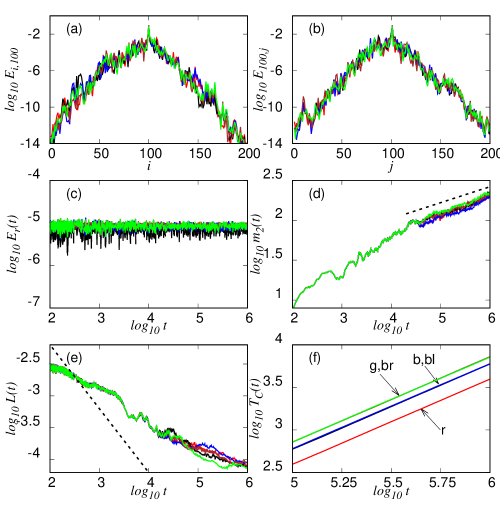
Figure 4: Results for the integration of case I of Hamiltonian (2) by the SIs $ABA864$ (order four) for $\tau=0.56$, $ABAH864$ (order four) for $\tau=0.40$, $SABA_{2}Y6$ (order six) for $\tau=0.60$, $s9SABA_{2}6$ (order six) for $\tau=0.60$, $ABA864Y6$ (order six) for $\tau=0.68$ [(r) red; (b) blue; (bl) black; (br) brown; (g) green]. The logarithm of the normalized energy distribution (a) $E_{i,100}$ and (b) $E_{100,j}$ at time $t_{f}=10^{6}$ as a function of the lattice site index $i$ and $j$ respectively. The time evolution of the logarithm of (c) $E_{r}(t)$, (d) $m_{2}(t)$, (e) $L(t)$ and (f) $T_{C}(t)$. Panels (c), (d), (e) and (f) are in $\log-\log$ scale. The straight dashed line in (d) guides the eye for slope $0.2$, while in (e) for slope $-1$. In (f) the curves for $ABAH864$, $SABA_{2}Y6$ and $s9SABA_{2}6$, $ABA864Y6$ practically overlap each other.

As the energy propagation takes place on a two-dimensional plane it is difficult to visualize in a comparative way the energy distributions obtained by the different integrators. For this reason we present in Fig. 4(a) the energy profiles along the $i$ axis for sites having $j=100$ and in Fig. 4(b) along the $j$ axis for sites with $i=100$ at $t_{f}=10^{6}$. We clearly see that the profiles produced by the different integrators practically coincide. Another piece of evidence that all schemes provide the same results is the fact that very nearly they produce the same time evolution of $m_{2}(t)$ [Fig. 4(d)], $P(t)$ (not shown) and $L(t)$ [Fig. 4(e)]. From Fig. 4(d) we see that eventually $m_{2}(t)\propto t^{0.2}$ in agreement with the results presented in LBF12 for the weak chaos case.

The evolution of $L(t)$ in Fig. 4(e) shows a power law decrease but with a rate which is completely different than the $L(t)\propto t^{-1}$ decay [dashed line in Fig. 4(e)] observed in the case of regular motion. This behavior indicates that the motion becomes less chaotic in time but without showing any sign of a crossover to regular dynamics. This is similar to what has been observed in the case of weak chaos of the 1D KG system SGF13 [see also Figs. 2(a) and 3(c)], where $L(t)\propto t^{-1/4}$. Fig. 4(e) suggests that $L(t)\propto t^{-\nu}$ with $\nu>0$ and $\nu\neq 1$, also for the 2D KG case, but the presented results are not enough to provide an accurate estimation for $\nu$ as they are based only on one disorder realization. A more detailed investigation of the evolution of $L(t)$ for larger integration times and many more disorder realizations and values of the system’s parameters (e.g. total energy and disorder strength) is needed. We plan to address this issue in a future publication.

From Fig. 4(f) we see that, as in the case of the 1D KG model (Fig. 2), the best performing scheme is the SI $ABA864$ followed by the $ABAH864$, $SABA_{2}Y6$ and $s9SABA_{2}6$, $ABA864Y6$ schemes, which behave similarly as their $T_{C}(t)$ vs. time curves practically overlap. We also note that similar results to the ones presented in Fig. 4 were also obtained for cases II and III, showing again that the most efficient integration scheme is the fourth order SI $ABA864$.

5 Summary and conclusions

We carried out a detailed analysis of the performance of several SIs, with orders ranging from two up to eight, for the long time integration of the equations of motion and the variational equations of the 1D (1) and the 2D (2) KG models. By performing extensive numerical simulations we investigated the ability of 33 SIs to correctly capture the characteristics of energy propagation induced by different initial excitations in these models, as well as to accurately quantify the systems’ chaoticity. In particular, we followed the time evolution of energy distributions and computed their second moment and participation number along with the corresponding finite time mLCE, by implementing each one of these SIs, registering also the CPU time they required. Our results show that the behavior of the tested SIs does not depend on the nature of the used initial excitations or the considered dynamical regime of the two lattice models.

For both models the integrators $ABA864$, $ABAH864$ of order four and $SABA_{2}Y6$, $s9SABA_{2}6$, $ABA864Y6$ of order six, exhibited the best performance when a moderate accuracy in the numerical conservation of the system’s energy was required (i.e. the corresponding absolute relative energy error was $E_{r}\approx 10^{-5}$), with $ABA864$ BCFLMM13 being always the most efficient one as it required the least CPU time. This is indeed a very efficient SI as also three part split symplectic schemes based on it showed the best performance among several SIs tested for the integration of the DNLS system SGBPE14 ; GMS16 . Thus, we propose that the $ABA864$ SI should be preferred for the long time integration of the 1D and 2D KG models over SIs of the $SABA$ family LR01 which have been extensively used to date for such studies FKS09 ; SKKF09 ; SF10 ; LBKSF10 ; BLSKF11 ; LBF12 . This is a basic outcome of our study, which can be of practical importance for researchers working on lattice dynamics of disordered and non-disordered systems.

Many of the considered sixth and eight order SIs were not able to produce reliable results for $E_{r}\approx 10^{-5}$ because the required integration time step $\tau$ needed for that purpose was rather high and made them unstable. These higher order SIs can be used in cases where an even better accuracy is required than the typically acceptable level of $E_{r}\approx 10^{-5}$ used in disordered lattice studies. For $E_{r}\approx 10^{-8}$ the best performing schemes were the SIs $s11ABA82\_6$, $SABA_{2}Y6$, $s9ABA82\_6$ of order six and $s15ABA82\_8$, $s19ABA82\_8$ of order eight, with $s11ABA82\_6$ being the most efficient one.

In our study we paid much attention to the integration of the variational equations by SIs based on the ‘tangent map method’ SG10 ; GS11 ; GES12 , because through their solution we can evaluate the mLCE and quantify the system’s chaoticity. For this reason we provide in the Appendix the explicit formulas of the operators needed for this task, both for the rather simple 1D KG system and the more complicated case of the 2D KG model. Our results indicate that it is possible to obtain the long time evolution of the finite time mLCE in feasible CPU times for both the 1D and the 2D KG systems. For the 2D KG system in particular, we evaluated the mLCE obtaining some numerical evidences (to the best of our knowledge for the first time) that in the weak chaos regime the mLCE decreases to zero following a power law which is different than the $t^{-1}$ law encountered for regular orbits. This behavior is similar to what has been observed also in the 1D KG case SGF13 . A more detailed investigation of the behavior of the mLCE for the different dynamical regimes appearing in the 2D KG model is needed in order to derive reliable conclusions for the system’s chaoticity, something we plan to address in the near future. The SIs presented in our work can facilitate the realization of this goal as they managed to speed up considerably the needed computations.

Appendix A The $e^{\tau L_{AV}}$ and $e^{\tau L_{BV}}$ operators

We present here the explicit form of operators $e^{\tau L_{AV}}$ and $e^{\tau L_{BV}}$ used for the time propagation of an orbit and a deviation vector with initial conditions $(\vec{q},\vec{p},\vec{\delta q},\vec{\delta p})$ at time $t_{0}$ to their final values $(\vec{q}^{\prime},\vec{p}^{\prime},\vec{\delta q}^{\prime},\vec{\delta p}^{\prime})$ at time $t_{0}+\tau$ for Hamiltonians (1) and (2).

A.1 The one-dimensional KG model

The equations of motion of the 1D KG model (1) are

$$\begin{array}[]{lll}\displaystyle\frac{dq_{i}}{dt}&=&\displaystyle p_{i},\,\,\,\mbox{for}\,\,\,1\leq i\leq N\\ \displaystyle\frac{dp_{1}}{dt}&=&\displaystyle-\left[\epsilon_{1}q_{1}+q_{1}^{3}+\frac{1}{W}\left(2q_{1}-q_{2}\right)\right]\\ \displaystyle\frac{dp_{i}}{dt}&=&\displaystyle-\left[\epsilon_{i}q_{i}+q_{i}^{3}+\frac{1}{W}\left(2q_{i}-q_{i-1}-q_{i+1}\right)\right],\,\,\,\mbox{for}\,\,\,2\leq i\leq N-1\\ \displaystyle\frac{dp_{N}}{dt}&=&\displaystyle-\left[\epsilon_{N}q_{N}+q_{N}^{3}+\frac{1}{W}\left(2q_{N}-q_{N-1}\right)\right],\end{array}$$ (17)

while the corresponding variational equations (14) have the form

$$\begin{array}[]{lll}\displaystyle\frac{d\delta q_{i}}{dt}&=&\displaystyle\delta p_{i},\,\,\,\mbox{for}\,\,\,1\leq i\leq N\\ \displaystyle\frac{d\delta p_{1}}{dt}&=&\displaystyle-\left[\delta q_{1}\left(\epsilon_{1}+3q_{1}^{2}\right)+\frac{1}{W}\left(2\delta q_{1}-\delta q_{2}\right)\right]\\ \displaystyle\frac{d\delta p_{i}}{dt}&=&\displaystyle-\left[\delta q_{i}\left(\epsilon_{i}+3q_{i}^{2}\right)+\frac{1}{W}\left(2\delta q_{i}-\delta q_{i-1}-\delta q_{i+1}\right)\right],\,\,\,\mbox{for}\,\,\,2\leq i\leq N-1\\ \displaystyle\frac{d\delta p_{N}}{dt}&=&\displaystyle-\left[\delta q_{N}\left(\epsilon_{N}+3q_{N}^{2}\right)+\frac{1}{W}\left(2\delta q_{N}-\delta q_{N-1}\right)\right].\end{array}$$ (18)

In order to implement the SIs of Sect. 3 for the simultaneous integration of equations (17) and (18) we split Hamiltonian (1) in two integrable parts

$$A_{1}(\vec{p})=\sum_{i=1}^{N}\frac{p_{i}^{2}}{2}\,,\,\,\,\,\,\,B_{1}(\vec{q})=\sum_{i=1}^{N}\left[\frac{\epsilon_{i}}{2}q_{i}^{2}+\frac{q_{i}^{4}}{4}+\frac{1}{2W}\left(q_{i+1}-q_{i}\right)^{2}\right],$$ (19)

i.e. the system’s kinetic and potential energy respectively. The solution of the Hamilton equations of motion and the variational ones for Hamiltonians $A_{1}$ and $B_{1}$ are obtained through the action of the operators

$$e^{\tau L_{AV_{1}}}:\left\{\begin{array}[]{lll}\displaystyle q^{\prime}_{i}&=&\displaystyle q_{i}+\tau p_{i}\\ \displaystyle p^{\prime}_{i}&=&\displaystyle p_{i}\\ \displaystyle\delta q^{\prime}_{i}&=&\displaystyle\delta q_{i}+\tau\delta p_{i}\\ \displaystyle\delta p^{\prime}_{i}&=&\displaystyle\delta p_{i}\end{array}\right.,\,\,\,\mbox{for}\,\,\,1\leq i\leq N,$$ (20)

and

$$e^{\tau L_{BV_{1}}}:\left\{\begin{array}[]{lll}\displaystyle q^{\prime}_{i}&=&\displaystyle q_{i},\,\,\,\mbox{for}\,\,\,1\leq i\leq N\\ \displaystyle p^{\prime}_{1}&=&\displaystyle p_{1}-\tau\left[\epsilon_{1}q_{1}+q_{1}^{3}+\frac{1}{W}\left(2q_{1}-q_{2}\right)\right]\\ \displaystyle p^{\prime}_{i}&=&\displaystyle p_{i}-\tau\left[\epsilon_{i}q_{i}+q_{i}^{3}+\frac{1}{W}\left(2q_{i}-q_{i-1}-q_{i+1}\right)\right],\,\,\,\mbox{for}\,\,\,2\leq i\leq N-1\\ \displaystyle p^{\prime}_{N}&=&\displaystyle p_{N}-\tau\left[\epsilon_{N}q_{N}+q_{N}^{3}+\frac{1}{W}\left(2q_{N}-q_{N-1}\right)\right]\\ &&\\ \displaystyle\delta q^{\prime}_{i}&=&\displaystyle\delta q_{i},\,\,\,\mbox{for}\,\,\,1\leq i\leq N\\ \displaystyle\delta p^{\prime}_{1}&=&\displaystyle\delta p_{1}-\tau\left[\delta q_{1}\left(\epsilon_{1}+3q_{1}^{2}\right)+\frac{1}{W}\left(2\delta q_{1}-\delta q_{2}\right)\right]\\ \displaystyle\delta p^{\prime}_{i}&=&\displaystyle\delta p_{i}-\tau\left[\delta q_{i}\left(\epsilon_{i}+3q_{i}^{2}\right)+\frac{1}{W}\left(2\delta q_{i}-\delta q_{i-1}-\delta q_{i+1}\right)\right],\,\,\,\mbox{for}\,\,\,2\leq i\leq N-1\\ \displaystyle\delta p^{\prime}_{N}&=&\displaystyle\delta p_{N}-\tau\left[\delta q_{N}\left(\epsilon_{N}+3q_{N}^{2}\right)+\frac{1}{W}\left(2\delta q_{N}-\delta q_{N-1}\right)\right].\end{array}\right.$$ (21)

Note that the first half of the equations of operators (20) and (21) correspond respectively to the operators $e^{\tau L_{A_{1}}}$ and $e^{\tau L_{B_{1}}}$ needed for the integration of only the system’s equations of motion.

A.2 The two-dimensional KG model

The 2D KG Hamiltonian (2) can also be written as the sum of two integrable systems: the kinetic energy $A_{2}(\vec{p})$ and the potential energy $B_{2}(\vec{q})$. In this case the propagation operators for the solution of the equations of motion and the variational equations have more complicated forms with respect to the 1D case and are given by the following expressions

$$e^{\tau L_{AV_{2}}}:\left\{\begin{array}[]{lll}\displaystyle q^{\prime}_{i,j}&=&\displaystyle q_{i,j}+\tau p_{i,j}\\ \displaystyle p^{\prime}_{i,j}&=&\displaystyle p_{i,j}\\ \displaystyle\delta q^{\prime}_{i,j}&=&\displaystyle\delta q_{i,j}+\tau\delta p_{i,j}\\ \delta p^{\prime}_{i,j}&=&\displaystyle\delta p_{i,j}\end{array}\right.,\,\,\,\mbox{for}\,\,\,1\leq i\leq N,\,\,1\leq j\leq M,$$ (22)

and

$$e^{\tau L_{BV_{2}}}:\left\{\begin{array}[]{lll}\displaystyle q^{\prime}_{i,j}&=&\displaystyle q_{i,j},\,\,\,\mbox{for}\,\,\,1\leq i\leq N,\,\,1\leq j\leq M\\ \displaystyle p^{\prime}_{1,1}&=&\displaystyle p_{1,1}-\tau\left[\epsilon_{1,1}q_{1,1}+q_{1,1}^{3}+\frac{1}{W}\left(4q_{1,1}-q_{2,1}-q_{1,2}\right)\right]\\ \displaystyle p^{\prime}_{1,M}&=&\displaystyle p_{1,M}-\tau\left[\epsilon_{1,M}q_{1,M}+q_{1,M}^{3}+\frac{1}{W}\left(4q_{1,M}-q_{1,M-1}-q_{2,M}\right)\right]\\ \displaystyle p^{\prime}_{N,1}&=&\displaystyle p_{N,1}-\tau\left[\epsilon_{N,1}q_{N,1}+q_{N,1}^{3}+\frac{1}{W}\left(4q_{N,1}-q_{N-1,1}-q_{N,2}\right)\right]\\ \displaystyle p^{\prime}_{N,M}&=&\displaystyle p_{N,M}-\tau\left[\epsilon_{N,M}q_{N,M}+q_{N,M}^{3}+\frac{1}{W}\left(4q_{N,M}-q_{N-1,M}-q_{N,M-1}\right)\right]\\ \displaystyle p^{\prime}_{i,j}&=&\displaystyle p_{i,j}-\tau\left[\epsilon_{i,j}q_{i,j}+q_{i,j}^{3}+\frac{1}{W}\left(4q_{i,j}-q_{i-1,j}-q_{i,j-1}\right.\right.\\ &&\displaystyle\left.\left.-q_{i+1,j}-q_{i,j+1}\right)\bigg{]}\right.,\,\,\,\mbox{for}\,\,\,2\leq i\leq N-1,\,\,2\leq j\leq M-1\\ \displaystyle p^{\prime}_{i,1}&=&\displaystyle p_{i,1}-\tau\left[\epsilon_{i,1}q_{i,1}+q_{i,1}^{3}+\frac{1}{W}\left(4q_{i,1}-q_{i-1,1}-q_{i+1,1}-q_{i,2}\right)\right],\,\,\,\mbox{for}\,\,\,2\leq i\leq N-1\\ \displaystyle p^{\prime}_{i,M}&=&\displaystyle p_{i,M}-\tau\left[\epsilon_{i,M}q_{i,M}+q_{i,M}^{3}+\frac{1}{W}\left(4q_{i,M}-q_{i-1,M}-q_{i,M-1}-q_{i+1,M}\right)\right],\,\,\,\mbox{for}\,\,\,2\leq i\leq N-1\\ \displaystyle p^{\prime}_{1,j}&=&\displaystyle p_{1,j}-\tau\left[\epsilon_{1,j}q_{1,j}+q_{1,j}^{3}+\frac{1}{W}\left(4q_{1,j}-q_{1,j-1}-q_{2,j}-q_{1,j+1}\right)\right],\,\,\,\mbox{for}\,\,\,2\leq j\leq M-1\\ \displaystyle p^{\prime}_{N,j}&=&\displaystyle p_{N,j}-\tau\left[\epsilon_{N,j}q_{N,j}+q_{N,j}^{3}+\frac{1}{W}\left(4q_{N,j}-q_{N-1,j}-q_{N,j-1}-q_{N,j+1}\right)\right],\,\,\,\mbox{for}\,\,\,2\leq j\leq M-1\\ &&\\ \displaystyle\delta q^{\prime}_{i,j}&=&\displaystyle\delta q_{i,j},\,\,\,\mbox{for}\,\,\,1\leq i\leq N,\,\,1\leq j\leq M\\ \displaystyle\delta p^{\prime}_{1,1}&=&\displaystyle\delta p_{1,1}-\tau\left[\delta q_{1,1}\left(\epsilon_{1,1}+3q_{1,1}^{2}\right)+\frac{1}{W}\left(4\delta q_{1,1}-\delta q_{2,1}-\delta q_{1,2}\right)\right]\\ \displaystyle\delta p^{\prime}_{1,M}&=&\displaystyle\delta p_{1,M}-\tau\left[\delta q_{1,M}\left(\epsilon_{1,M}+3q_{1,M}^{2}\right)+\frac{1}{W}\left(4\delta q_{1,M}-\delta q_{1,M-1}-\delta q_{2,M}\right)\right]\\ \displaystyle\delta p^{\prime}_{N,1}&=&\displaystyle\delta p_{N,1}-\tau\left[\delta q_{N,1}\left(\epsilon_{N,1}+3q_{N,1}^{2}\right)+\frac{1}{W}\left(4\delta q_{N,1}-\delta q_{N-1,1}-\delta q_{N,2}\right)\right]\\ \displaystyle\delta p^{\prime}_{N,M}&=&\displaystyle\delta p_{N,M}-\tau\left[\delta q_{N,M}\left(\epsilon_{N,M}+3q_{N,M}^{2}\right)+\frac{1}{W}\left(4\delta q_{N,M}-\delta q_{N-1,M}-\delta q_{N,M-1}\right)\right]\\ \displaystyle\delta p^{\prime}_{i,j}&=&\displaystyle\delta p_{i,j}-\tau\left[\delta q_{i,j}\left(\epsilon_{i,j}+3q_{i,j}^{2}\right)+\frac{1}{W}\left(4\delta q_{i,j}-\delta q_{i-1,j}-\delta q_{i,j-1}\right.\right.\\ &&\displaystyle\left.\left.-\delta q_{i+1,j}-\delta q_{i,j+1}\right)\bigg{]}\right.,\,\,\,\mbox{for}\,\,\,2\leq i\leq N-1,\,\,2\leq j\leq M-1\\ \displaystyle\delta p^{\prime}_{i,1}&=&\displaystyle\delta p_{i,1}-\tau\left[\delta q_{i,1}\left(\epsilon_{i,1}+3q_{i,1}^{2}\right)+\frac{1}{W}\left(4\delta q_{i,1}-\delta q_{i-1,1}-\delta q_{i+1,1}-\delta q_{i,2}\right)\right],\,\,\,\mbox{for}\,\,\,2\leq i\leq N-1\\ \displaystyle\delta p^{\prime}_{i,M}&=&\displaystyle\delta p_{i,M}-\tau\left[\delta q_{i,M}\left(\epsilon_{i,M}+3q_{i,M}^{2}\right)+\frac{1}{W}\left(4\delta q_{i,M}-\delta q_{i-1,M}-\delta q_{i,M-1}-\delta q_{i+1,M}\right)\right],\,\,\,\mbox{for}\,\,\,2\leq i\leq N-1\\ \displaystyle\delta p^{\prime}_{1,j}&=&\displaystyle\delta p_{1,j}-\tau\left[\delta q_{1,j}\left(\epsilon_{1,j}+3q_{1,j}^{2}\right)+\frac{1}{W}\left(4\delta q_{1,j}-\delta q_{1,j-1}-\delta q_{2,j}-\delta q_{1,j+1}\right)\right],\,\,\,\mbox{for}\,\,\,2\leq j\leq M-1\\ \displaystyle\delta p^{\prime}_{N,j}&=&\displaystyle\delta p_{N,j}-\tau\left[\delta q_{N,j}\left(\epsilon_{N,j}+3q_{N,j}^{2}\right)+\frac{1}{W}\left(4\delta q_{N,j}-\delta q_{N-1,j}-\delta q_{N,j-1}-\delta q_{N,j+1}\right)\right],\,\,\,\mbox{for}\,\,\,2\leq j\leq M-1.\\ \end{array}\right.$$ (23)

References

- (1) P. W. Anderson, Phys. Rev. 109, 1492 (1958)
- (2) D. Shepelyansky, Phys. Rev. Lett. 70, 1787 (1993)
- (3) M. Molina, Phys. Rev. B 58, 12547 (1998)
- (4) D. Clément, A. F. Varón, M. Hugbart, J. A. Retter, P. Bouyer, L. Sanchez-Palencia, D. M. Gangardt, G. V. Shlyapnikov, A. Aspect, Phys. Rev. Lett. 95 170409 (2005)
- (5) C. Fort, L. Fallani, V. Guarrera, J. E. Lye, M. Modugno, D. S. Wiersma, M. Inguscio, Phys. Rev. Lett. 95 170410 (2005)
- (6) T. Schwartz, G. Bartal, S. Fishman, M. Segev, Nature 446, 52 (2007)
- (7) Y. Lahini, A. Avidan, F. Pozzi, M. Sorel, R. Morandotti, D. N. Christodoulides, Y. Silberberg, Phys. Rev. Lett. 100, 013906 (2008)
- (8) J. Billy, V. Josse, Z. Zuo, A. Bernard, B. Hambrecht, P. Lugan, D. Clément, L. Sanchez-Palencia, P. Bouyer, A. Aspect, Nature 453, 891 (2008)
- (9) G. Roati, C. D’Errico, L. Fallani, M. Fattori, C. Fort, M. Zaccanti, G. Modugno, M. Modugno, M. Inguscio, Nature 453, 895 (2008)
- (10) G. Kopidakis, S. Komineas, S. Flach, S. Aubry, Phys. Rev. Lett. 100, 084103 (2008)
- (11) A. S. Pikovsky, D. L. Shepelyansky, Phys. Rev. Lett. 100, 094101 (2008)
- (12) S. Flach, D. O. Krimer, Ch. Skokos, Phys. Rev. Lett. 102, 024101 (2009)
- (13) S. Flach, D. O. Krimer, Ch. Skokos, Phys. Rev. Lett. 102, 209903 (2009)
- (14) I. García-Mata, D. L. Shepelyansky, Phys. Rev. E 79, 026205 (2009)
- (15) Ch. Skokos, D. O. Krimer, S. Komineas, S. Flach, Phys. Rev. E 79, 056211 (2009)
- (16) H. Veksler, Y. Krivolapov, S. Fishman, Phys. Rev. E 80, 037201 (2009)
- (17) Ch. Skokos, S. Flach, Phys. Rev. E 82, 016208 (2010)
- (18) T. V. Laptyeva, J. D. Bodyfelt, D. O. Krimer, Ch. Skokos, S. Flach, Europhys. Lett. 91, 30001 (2010)
- (19) S. Flach, Chem. Phys. 375, 548 (2010)
- (20) D. M. Basko, Annals Phys. 326, 1577 (2011) (2014)
- (21) M. Mulansky, K. Ahnert, A. Pikovsky, Phys. Rev. E 83, 026205 (2011)
- (22) M. Mulansky, K. Ahnert, A. Pikovsky, D. L. Shepelyansky, J. Stat. Phys. 145, 1256 (2011)
- (23) J. D. Bodyfelt, T. V. Laptyeva, Ch. Skokos, D. O. Krimer, S. Flach, Phys. Rev. E 84, 016205 (2011)
- (24) J. D. Bodyfelt, T. V. Laptyeva, G. Gligoric, D. O. Krimer, Ch. Skokos, S. Flach, Int. J. Bifur. Chaos 21(8), 2107 (2011)
- (25) S. S. Kondov, W. R. McGehee, J. J. Zirbel, B. DeMarco, Science 334, 66 (2011)
- (26) T. V. Laptyeva, J. D. Bodyfelt, S. Flach, Europhys. Lett. 98, 60002 (2012)
- (27) M. Mulansky, A. Pikovsky, Phys. Rev. E 86, 056214 (2012)
- (28) F. Jendrzejewski, A. Bernard, K. Mueller, P. Cheinet, V. Josse, M. Piraud, L. Pezze, L. Sanchez-Palencia, A. Aspect, P. Bouyer, Nat. Phys. 8,398 (2012)
- (29) M. Mulansky, A. Pikovsky, New J. Phys. 15, 053015 (2013)
- (30) Ch. Skokos, I. Gkolias, S. Flach, Phys. Rev. Lett. 111, 064101 (2013)
- (31) Ch. Antonopoulos, T. Bountis, Ch. Skokos, L. Drossos, Chaos 24, 024405 (2014)
- (32) T. V. Laptyeva, M. V. Ivanchenko, S. Flach, J. Phys. A 47, 493001 (2014)
- (33) Ch. Skokos, D. O. Krimer, S. Komineas, S. Flach, Phys. Rev. E 89, 029907 (2014)
- (34) O. Tieleman, Ch. Skokos, A. Lazarides, Europhys. Lett. 105, 20001 (2014)
- (35) A. J. Martínez, P. G. Kevrekidis, M. A. Porter, Phys. Rev. E 93, 022902 (2016)
- (36) V. Achilleos, G. Theocharis, Ch. Skokos, Phys. Rev. E 93, 022903 (2016)
- (37) A. J. Martínez, H. Yasuda, E. Kim, P. G. Kevrekidis, M. A. Porter, J. Yang, Phys. Rev. E 93, 052224 (2016)
- (38) Ch. Antonopoulos, Ch. Skokos, T. Bountis, S. Flach, Chaos Sol. Fract. 104, 129 (2017)
- (39) C. Chong, M. A. Porter, P. G. Kevrekidis, C. Daraio, J. Phys. Cond. Matt 29, 413003 (2017)
- (40) S. Donsa, H. Hofstätter, O. Koch, J. Burgdörfer, I. Březinová, Phys. Rev. A 96 043630
- (41) V. Achilleos, G. Theocharis, Ch. Skokos [ArXiv:nlin.CD/1707.03162] (2017)
- (42) E. Hairer, C. Lubich, G. Wanner, Geometric Numerical Integration. Structure-Preserving Algorithms for Ordinary Differential Equations, Chap. VI (Springer Series in Computational Mathematics Vol. 31, Springer, New York, 2002)
- (43) R. I. McLachan, G. R. W. Quispel, Acta Num. 11, 341 (2002)
- (44) R. I. McLachan, G. R. W. Quispel, J. Phys. A 39, 5251 (2006)
- (45) E. Forest, J. Phys. A 39, 5321 (2006)
- (46) S. Blanes, F. Casas, A. Murua, Bol. Soc. Esp. Mat. Apl. 45, 89 (2008)
- (47) Ch. Skokos, E. Gerlach, J. D. Bodyfelt, G. Papamikos, S. Eggl, Phys. Lett. A 378, 1809 (2014)
- (48) E. Gerlach, J. Meichsner, Ch. Skokos, Eur. Phys. J. Sp. Top. 225, 1103 (2016)
- (49) J. Laskar, P. Robutel, Cel. Mech. Dyn. Astr. 80, 39 (2001)
- (50) Ch. Skokos, G. A. Gottwald, J. Laskar, in Lecture Notes in Physics, Berlin Springer Verlag, Vol. 915, Chaos Detection and Predictability, (2016)
- (51) G. Benettin, L. Galgani, A. Giorgilli, J.-M. Strelcyn, Meccanica 15, 9 (1980)
- (52) G. Benettin, L. Galgani, A. Giorgilli, J.-M. Strelcyn, Meccanica 15, 21 (1980)
- (53) Ch. Skokos, Lect. Notes Phys. 790, 63 (2010)
- (54) R. D. Ruth, IEEE Trans. Nucl. Sci. 30, 2669 (1983)
- (55) R. I. Mclachlan, BIT 35, 258 (1995)
- (56) A. Farres, J. Laskar, S. Blanes, F. Casas, J. Makazaga, A. Murua, Cel. Mech. Dyn. Astr. 116, 141 (2013)
- (57) H. Yoshida, Phys. Let. A 150, 262 (1990)
- (58) E. Forest, R. D. Ruth, Phys. D. 43, 105 (1990)
- (59) S. Blanes, F. Casas, A. Farres, J. Laskar, J. Makazaga, A. Murua, App. Num. Math. 68, 58 (2013)
- (60) W. Kahan, R. Li, Math. Comp. 66, 1089 (1997)
- (61) M. Sofroniou, G. Spaletta, Opt. Meth. Soft. 20, 597 (2005)
- (62) G. Benettin, L. Galgani, J.-M. Strelcyn, Phys. Rev. A 14, 2338 (1976)
- (63) Ch. Skokos, E. Gerlach E., Phy. Rev. E 82, 036704 (2010)
- (64) E. Gerlach, Ch. Skokos, Discr. Cont. Dyn. Sys.-Supp. 475 (2011)
- (65) E. Gerlach, S. Eggl, Ch. Skokos, Int. J. Bifur. Chaos 22, 1250216 (2012)