OU-HET 956

Mixed global anomalies and boundary conformal field theories
Tokiro Numasawa ${}^{1,2}$ and Satoshi Yamaguchi${}^{1}$

${}^{1}$ Department of Physics, Graduate School of Science,
Osaka university, Toyonaka 560-0043, Japan ${}^{2}$ Department of Physics, McGill University,
3600 rue University, Montréal, Québec, Canada H3A 2T8

We consider the relation between mixed global gauge gravitational anomalies and boundary conformal field theory in WZW models for simple Lie groups. The discrete symmetries of consideration are the centers of the simple Lie groups. These mixed anomalies prevent gauging them i.e, taking the orbifold by the center. The absence of anomalies impose conditions on the levels of WZW models. Next, we study the conformal boundary conditions for the original theories. We consider the existence of a conformal boundary state invariant under the action of the center. This also gives conditions on the levels of WZW models. By considering the combined action of the center and charge conjugation on boundary states, we reproduce the condition obtained in the orbifold analysis.

1 Introduction

A ’t Hooft anomaly is an obstruction to gauge a global symmetry, and puts a constraint on the RG flows called ’t Hooft anomaly matching condition[tHooft]; the ’t Hooft anomaly of the IR theory matches with that of the UV theory as long as the theory has the global symmetry in question during the RG flow. This matching condition can also be applied to discrete symmetries[CsMu].

Recently, quantum anomalies are focus of attention in condensed matter physics, because they provide a useful tool to investigate symmetry protected topological (SPT) phases[CGLW]. When we put a theory in a non-trivial SPT phase on a manifold with boundaries, the boundary localized modes with ’t Hooft anomalies appear. They are now coupled to the bulk theory and ’t Hooft anomalies are canceled in the same manner as the usual anomaly inflow mechanism[CaHa].

The study of SPT phases gives a natural motivation to consider the anomalies of discrete symmetries and global anomalies. In the cases of perturbative anomalies we have them in the system with chiral fields in even dimensions. On the other hand, anomalies of discrete symmetries and global anomalies can also exist in non-chiral, bosonic systems in odd dimensions. Recently the anomalies for discrete symmetries are focus of attention[KaTh1][KaTh2], generalized to $p$-form symmetries[GKSW][ThKe], and applied to the study of non-supersymmetric gauge theories[GKKS][TaKi][ShYo]. In this paper, we consider the mixed anomalies between large diffeomorphisms and discrete symmetries. The continuum counterpart of this mixed anomaly does not exist in $1+1$ dimensions because such mixed term can not appear in anomaly polynomials.

Another application of a ’t Hooft anomaly in condensed matter physics is to use itself as a classification of a gapless version of an SPT phase[FuOs]. If two theories have different ’t Hooft anomalies for a symmetry $\Gamma$, they cannot be connected by RG flows while preserving the symmetry $\Gamma$ and thus they are in different symmetry protected phases. In this manner, we can use the ’t Hooft anomalies to detect both $(2+1)$-dimensional SPT phases[CGLW] and $(1+1)$-dimensional symmetry protected critical phases[FuOs].

In conformal field theory, the procedure to gauge a discrete global symmetry $\Gamma$ is known as the orbifold construction. In this procedure, we exclude the non-invariant states under $\Gamma$ action (i.e. project the spectrum onto the invariant states) and also need to include the twisted sector (soliton sector) to preserve the modular invariance, which is the invariance under a class of large diffeomorphisms. Once we determine the way to project onto the invariant states, the modular invariance determines the twisted sector and the projection operation on it. Sometimes the twisted sector determined from modular invariance is not compatible with the action of the symmetry $\Gamma$ and causes inconsistency. This inconsistency is the mixed anomaly between large diffeomorphisms (modular transformations $\mathrm{SL}(2,\mathbb{Z})$) and the symmetry $\Gamma$ .

The related constraints to the modular invariance are the consistency of boundary conformal field theories[Cardy]. There are several motivation to consider the relation between ’t Hooft anomalies and boundary states.

First, one way to distinguish SPT phases is putting a theory on a non-trivial background[GKKS], and another way is putting the theory on a manifold with boundary[CGLW, AKLT1, AKLT2]. For example, we can find that the spin $1$ Haldane chain, whose phase is realized in the Affleck-Kennedy-Lieb-Tasaki (AKLT) model[AKLT1, AKLT2], is in a non-trivial phase by putting the theory on a non-trivial monopole background (non-trivial Stiefel-Whitney class)[GKKS] or putting the theory on a manifold with a boundary[Kennedy][CGLW]. Now, we can think of an ’t Hooft anomaly itself as a classification of a gapless version of a SPT phase[FuOs]. Therefore, it should be useful to consider the analog of them in CFTs. The analog of the former is putting a theory on a non-trivial gauge-gravitational background. The analog of the latter is to consider the CFTs with boundaries. The natural boundary conditions are conformal boundary conditions, which keep the half of full conformal symmetry.

Second motivation is that in some cases we can detect $(2+1)$-dimensional SPT phases ($(1+1)$-dimensional ’t Hooft anomalies) from boundary states [HTHR, Bultinck:2017iff]. According to [HTHR, Bultinck:2017iff], if we find Cardy states invariant under symmetry transformations, the symmetry is anomaly free and they do not corresponds to the edge theory of non-trivial SPT phases. On the other hand, if we cannot construct such boundary states, the symmetry has ’t Hooft anomalies. This condition seems to be closely related to construction of the twisted sectors.

These consideration brings us to study the symmetry property of boundary conformal field theories. In this paper we consider the ’t Hooft anomaly in WZW models for Lie groups $G$ whose center $\Gamma$ is a cyclic group. We consider the anomaly of the center $\Gamma$. Here we give a brief summary of this paper. Depending on the level $k$ and groups $G$, the orbifold theory by $\Gamma$ may not be compatible with modular invariance, i.e. the large diffeomorphisms on a torus. This can be understood as a mixed anomaly between the large differmorphisms and the center $\Gamma$. Next, we study the existence of invariant boundary conditions under the center $\Gamma$ in the original WZW models with diagonal modular invariants for simple Lie groups $G$. This also depends on the level $k$ and sometimes there are no such boundary states. Surprisingly, these conditions obtained in the boundary state analysis perfectly match with the conditions obtained in the orbifold analysis for the simple group $G$ that does not have complex representations. For simple Lie groups $G$ with complex representations $(A_{n},D_{2l+1},E_{6})$, we consider the conditions for the existence of invariant boundary states under combined action of the generator $h\in\Gamma$ and charge conjugation $C$. These conditions match with the conditions obtained in the orbifold analysis for these groups.

The rest of this paper is organized as follows. In Section 2, we summarize how mixed global gauge gravitational anomalies appear in $(1+1)$-dimensional CFTs. Only when this mixed anomalies are absent, we can take the orbifold. Then, we review the case of the WZW model of Lie group $G$. We consider the orbifold by the center and its subgroup. We also show some examples of anomaly cancellation between two WZW models. In section LABEL:sec:BCFT, we study the condition to find a symmetry invariant boundary state. We show that we can find the same condition with the orbifold analysis.

2 Mixed global anomalies and orbifold constructions in CFTs

2.1 Coupling to external discrete gauge fields and mixed anomalies

In this section, we consider the mixed gauge gravitational anomalies in $(1+1)$-dimensional CFTs. This is nothing but the condition for the consistency of orbifold [FrVa][FGK][SCR]. We review these results, emphasizing the point that mixed global gauge gravitational anomalies appear.

Let us consider a cyclic symmetry $\Gamma$ of order $N$ and its orbifold. We consider the theory on a torus with modulus $\tau$. First, we consider coupling the original theory to “external gauge field,” which means nontrivial twisted boundary conditions by $\Gamma$. Because we consider CFTs on a torus, we can consider a twisted boundary condition on each direction. We denote this boundary condition by $(h_{t},h_{x})$ where $h_{t},h_{x}\in G$ denote the group elements to put the twisted boundary condition in imaginary time direction $t$ and space direction $x$ respectively. In other words, the boundary condition for the fields $g(z,\bar{z})$ are given by

$$g(z+1,\bar{z}+1) = h_{x}g(z,\bar{z}),$$

$$g(z+\tau,\bar{z}+\bar{\tau}) = h_{t}g(z,\bar{z}).$$ (2.1)

Partition functions with these twists are denoted as $Z_{(h_{t},h_{x})}$. In operator formalism, $Z_{(h,\bf{1})}$ corresponds to the partition function with symmetry action $\text{Tr}(h\,e^{-2\pi\text{Im}\tau H}e^{i2\pi\text{Re}\tau P})$. On the other hand, $Z_{(\bm{1},h)}$ corresponds to the twisted sector partition function without the projection onto the gauge invariant states.

Next we consider modular transformations, which are the large diffeomorphisms on a torus. Modular transformations $\mathrm{SL}(2,\mathbb{Z})$ are generated by $S=\begin{pmatrix}0&-1\\ 1&0\end{pmatrix}$ and $T=\begin{pmatrix}1&1\\ 1&0\end{pmatrix}$. We denote the action of $T,S\in\mathrm{SL}(2,\mathbb{Z})$ on a partition function $Z$ by $\mathcal{T}Z$ and $\mathcal{S}Z$. The boundary condition $(h_{t},h_{x})$ is mapped to $(h_{t}^{a}h_{x}^{b},h_{t}^{c}h_{x}^{d})$ by the modular transformation $\tau\to\frac{a\tau+b}{c\tau+d}$ labeled by $M=\begin{pmatrix}a&b\\ c&d\end{pmatrix}\in\mathrm{SL}(2,\mathbb{Z})$ . See for example[FuOs][FrVa].

If we assume this $\mathrm{SL}(2,\mathbb{Z})$ large diffeomorphism invariance, partition functions $Z_{(h_{t},h_{x})}$ are related to each other by modular transformations according to the map of boundary conditions $(h_{t},h_{x})\to(h_{t}^{a}h_{x}^{b},h_{t}^{c}h_{x}^{d})$. Especially, this means $Z_{(\bm{1},h)}=\mathcal{S}Z_{(h,\bm{1})}$ and $Z_{(h^{l},h)}=\mathcal{T}^{l}\mathcal{S}Z_{(h,\bm{1})}$. The first equation means that the twisted sector partition function $Z_{(\bm{1},h)}$ is determined by symmetry action $\text{Tr}(h\,e^{-2\pi\text{Im}\tau H}e^{i2\pi\text{Re}\tau P})$ and its modular $S$ transformation. The second equation means that the action of $\Gamma$ on the twisted sector is determined by the modular $T$ transformation.

The orbifold partition function is given by summing over the “external gauge background” configurations. The summation over independent discrete gauge background is given by

$$Z_{orb}=\frac{1}{|\Gamma|}\sum_{h_{t},h_{x}\in\Gamma}Z_{(h_{t},h_{x})},$$ (2.2)

where $|\Gamma|$ is the order of $\Gamma$ and corresponds to the gauge volume.

Until now we assumed that there are no anomalies. Let us see how the above procedure fails when mixed anomalies exist. An inconsistency can happens from the condition $Z_{(h^{l},h)}=\mathcal{T}^{l}\mathcal{S}Z_{(h,\bm{1})}$. Especially, we will see that in some cases $\mathcal{T}^{N}\mathcal{S}Z_{(h,\bm{1})}=Z_{(h^{N},h)}=Z_{(\bm{1},h)}$ is not satisfied but pick a phase factor $e^{i\theta}Z_{(\bm{1},h)}$. This means that the action of $h\in\Gamma$ on twisted sector determined from modular transformation actually does not satisfy $h^{N}=1$. This non-trivial phase factor breaks the invariance under the transformation $g(z,\bar{z})\to h^{N}g(z,\bar{z})$, which is actually the identity transformation [SCR]. Therefore, the orbifold construction (2.2) does not work in this case.

2.2 $\mathrm{SU}(2)_{k}$ WZW models

Here we consider the mixed global anomalies in $\mathrm{SU}(2)_{k}$ WZW models considered in [FuOs][GeWi]. $\mathrm{SU}(2)_{k}$ WZW models have $k+1$ primary fields which are labeled by the spin $0\leq j\leq\frac{k}{2}$. The Lagrangian of this theory is given by[Yellow]

$$S=\frac{|k|}{8\pi}\int dtdx\ \text{Tr}[\partial_{\mu}g\partial^{\mu}g^{-1}]+\frac{k}{12\pi}\int_{M_{3}}\text{Tr}[(\tilde{g}^{-1}d\tilde{g})^{3}],$$ (2.3)

where $g(t,x)$ takes the value on the $\mathrm{SU}(2)$ group manifold and $M_{3}$ in the second term is a $3$-dimensional manifold whose boundary is the spacetime we are considering. $\tilde{g}$ is an extension of $g$ to $M_{3}$. In order to be independent from the choice of $M_{3}$ and $\tilde{g}$, $k$ must be quantized correctly i.e. $k\in\mathbb{Z}$. From now we only consider non-negative $k$.

In the diagonal theory, we have $k+1$ primary states $\ket{j,j}$ for $0\leq j\leq\frac{k}{2}$. The action of the center $\Gamma=\mathbb{Z}_{2}=\{\bm{1},h\}$ is given by $h\ket{j,j}=(-1)^{2j}\ket{j,j}$. The partition function of the diagonal theory is given by

$$Z_{diag}=Z_{(\bm{1},\bm{1})}=\sum_{j\in\frac{1}{2}\mathbb{Z}}^{\frac{k}{2}}|\chi_{j}|^{2},$$ (2.4)

where $\chi_{j}$ is the character of the family including the primary state labeled by $j$. Let us consider the partition functions with twisted boundary conditions. First we consider the partition function $Z_{(h,\bm{1})}=\text{Tr}(h\ e^{-2\pi\text{Im}\tau H}e^{i2\pi\text{Re}\tau P})$. This partition function is given by

$$Z_{(h,\bm{1})}=\sum_{j\in\frac{1}{2}\mathbb{Z}}^{\frac{k}{2}}(-1)^{2j}|\chi_{j}|^{2}.$$ (2.5)

The modular $S$ matrix and $T$ matrix are given by

$$S_{jj^{\prime}} = \sqrt{\frac{2}{k+2}}\sin\frac{\pi(2j+1)(2j^{\prime}+1)}{k+2},$$

$$T_{jj^{\prime}} = e^{2\pi i(\Delta_{j}-\frac{c}{24})}\delta_{jj^{\prime}},$$ (2.6)

where $\Delta_{j}=\frac{j(j+1)}{k+2}$ and $c=\frac{3k}{k+2}$.

Let us assume modular invariance and see if any contradiction appears. Using (2.6), we can compute $\mathcal{S}Z_{(h,\bm{1})}=Z_{(\bm{1},h)}$ and $\mathcal{T}^{l}\mathcal{S}Z_{(h,\bm{1})}=Z_{(h^{l},h)}$ directly. The result is given by

$$Z_{(\bm{1},h)} = \sum_{j\in\frac{1}{2}\mathbb{Z}}^{\frac{k}{2}}\chi_{j}\bar{\chi}_{\frac{k}{2}-j},$$

$$Z_{(h^{l},h)} = \sum_{j\in\frac{1}{2}\mathbb{Z}}^{\frac{k}{2}}(-i)^{kl}(-1)^{2jl}\chi_{j}\bar{\chi}_{\frac{k}{2}-j}.$$ (2.7)

Especially, we obtain $Z_{(h^{2},h)}=(-1)^{k}Z_{(\bm{1},h)}$. Since $h^{2}=\bm{1}$, we find a contradiction when $k$ is an odd number. In other words, the theory has a mixed global ’t Hooft anomaly when $k$ is an odd number.

We can compute orbifold partition function (2.2) using (2.7) when $k$ is an even number. The results are given by[FuOs][GeWi]

$$Z_{orb}=\sum_{\begin{subarray}{c}j=0\\ j\in\mathbb{Z}\end{subarray}}^{\lfloor\frac{k}{2}\rfloor}|\chi_{j}|^{2}+\sum_{\begin{subarray}{c}j=0\\ j\in\frac{1}{2}\mathbb{Z}\end{subarray}}^{\frac{k}{2}}\frac{1+(-i)^{k}(-1)^{2j}}{2}\chi_{j}\bar{\chi}_{\frac{k}{2}-j}.$$ (2.8)

When $k=4l\ (l\in\mathbb{Z})$, this gives so called $D_{2l}$ type modular invariants:

$$Z_{orb}=\sum_{\begin{subarray}{c}j=0\\ j\in\mathbb{Z}\end{subarray}}^{l-1}|\chi_{j}+\chi_{2l-j}|^{2}+2|\chi_{l}|^{2}.$$ (2.9)

On the other hand, when $k=4l+2$, $Z_{orb}$ becomes so called $D_{2l+1}$ type modular invariants:

$$Z_{orb}=\sum_{\begin{subarray}{c}j=0\\ j\in\mathbb{Z}\end{subarray}}^{2l+1}|\chi_{j}|^{2}+|\chi_{l+\frac{1}{2}}|^{2}+\sum_{\begin{subarray}{c}j=\frac{1}{2}\\ j\in\mathbb{Z}+\frac{1}{2}\end{subarray}}^{l-\frac{1}{2}}(\chi_{j}\bar{\chi}_{2l+1-j}+\bar{\chi}_{j}\chi_{2l+1-j}).$$ (2.10)

Finally we give a comment on a difference between $k=4l$ and $k=4l+2$. Actually, $D_{2l+1}$ type modular invariants contain half odd spins while $D_{2l}$ type modular invariants do not. This mod $4$ structure comes from the phase factor $(-i)^{k}$ in $Z_{(h,h)}$. See eq. (2.7) . This is related to the consistency of the $\mathrm{SO}(3)$ Chern-Simons (CS) theory[DiWi]. A level of Chern Simons theory is quantized depending on the least instanton number in $4$ dimensions[DiWi]. In $\mathrm{SO}(3)$ cases, the instanton number is a multiple of $\frac{1}{4}$. Therefore, the level $k$ of an $\mathrm{SO}(3)$ CS theory is quantized to a multiple of $4$ in $\mathrm{SU}(2)$ language. On the other hand, if we consider spin Chern-Simons theories, the quantization condition is changed and levels $k=4l+2$ are allowed[DiWi].

2.3 General WZW model for simple Lie group $G$

In this subsection we consider the WZW model for a simple Lie group $G$. The consistency condition for the orbifold by the center of $G$ has been studied [AhWa][FGK][GaSc][Gaberdiel]. In this subsection we summarize these results. We follow the notations and the conventions of [Yellow] unless otherwise stated.

Let us see these conditions from the perspective of mixed global anomalies. We consider the case that the center $\Gamma$ of $G$ is a cyclic group $\mathbb{Z}_{N}$. In WZW models for general Lie groups $G$, the Lagrangian is given in the similar way to (2.3). The primaries are labeled by a set of non-negative integers, called affine Dynkin labels, $\hat{\lambda}=[\lambda_{0};\lambda_{1},\cdots,\lambda_{r}]$ where $r$ is the rank of $G$ with the condition. The level $k$ is related to $\hat{\lambda}$ by

$$k=\lambda_{0}+\sum_{i=1}^{r}a_{i}^{\vee}\lambda_{i},$$ (2.11)

where $a_{i}^{\vee},\ i=1,\cdots,r$ are the comarks of the corresponding Lie algebra. Our convention for the labels of the simple roots is the same as [Yellow]. The labels of the simple roots and the comarks of the relevant Lie algebras are summarized in Figure 1. The non-negativity of $\lambda_{0}$ and the relation (2.11) give a constraint on the allowed representations:

$$0\leq\sum_{i=1}^{r}a_{i}^{\vee}\lambda_{i}\leq k.$$ (2.12)

$P_{+}^{k}$ denotes the set of affine Dynkin labels which satisfy the above condition.

$A_{r},\quad r\geq 2$	$D_{r},\quad r\geq 4$
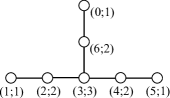
$B_{r},\quad r\geq 3$	$E_{6}$
$C_{r},\quad r\geq 2$	$E_{7}$

Figure 1: The extended Dynkin diagrams and the comarks of the relevant Lie algebras. The symbol $(i;a_{i}^{\vee})$ at each node denotes the label of the corresponding simple root and the comark. Each black node $\bullet$ corresponds to a short root, while each white node $\circ$ corresponds to a long root.

We consider the center group $\mathbb{Z}_{N}=\{\bm{1},h,\cdots,h^{N-1}\}$ generated by $h$. The action of $h$ is given by the following equation [Yellow]:

$$h\ket{\hat{\lambda},\hat{\lambda}}=e^{-2\pi i(A\hat{\omega}_{0},\lambda)}\ket{\hat{\lambda},\hat{\lambda}}.$$ (2.13)

We also use $h$ to represent the matrix whose elements are given by $h_{\hat{\mu},\hat{\lambda}}=e^{-2\pi i(A\hat{\omega}_{0},\lambda)}\delta_{\hat{\mu},\hat{\lambda}}$.

Another important operation is the action of outer automorphisms of the affine Lie algebra $\hat{\mathfrak{g}}$. The action of the generator $A$ of outer automorphisms on a character is induced from the action on the weight lattice:

$$A\chi_{\hat{\lambda}}=\chi_{A\hat{\lambda}}.$$ (2.14)

In the matrix notation, we can represent $A_{\hat{\mu},\hat{\lambda}}=\delta_{\hat{\mu},A\hat{\lambda}}$ where the action of matrices is defined by $A\chi_{\hat{\lambda}}=\sum_{\hat{\mu}}\chi_{\hat{\mu}}A_{\hat{\mu},\hat{\lambda}}$. The center of $G$ is isomorphic to outer automorphisms of the corresponding affine Lie algebra $\hat{\mathfrak{g}}$. Actually, the isomorphism is given by the modular S matrix as

$$SAS^{\dagger}=h.$$ (2.15)

In the matrix form, we can represent this as $(SAS^{\dagger})_{\hat{\mu},\hat{\lambda}}=\sum_{\hat{\sigma},\hat{\rho}}S_{\hat{\lambda},\hat{\sigma}}A_{\hat{\sigma},\hat{\rho}}(S^{\dagger})_{\hat{\rho},\hat{\mu}}$ . Here we introduce modular S matrix $S_{\hat{\mu},\hat{\lambda}}$ by $\mathcal{S}\chi_{\hat{\lambda}}=\sum_{\hat{\mu}}\chi_{\hat{\mu}}S_{\hat{\mu},\hat{\lambda}}$.

We employ the same strategy as $\mathrm{SU}(2)$ case; we assume the modular invariance and see if any contradiction appears. Then the twisted sector partition function (before the projection onto gauge invariant states) is given by the outer automorphism of $\hat{\mathfrak{g}}$:

$$Z_{(\bm{1},h)}=\mathcal{S}Z_{(h,\bm{1})}=\sum_{\hat{\mu}\in P_{+}^{k}}\bar{\chi}_{A\hat{\mu}}\chi_{\hat{\mu}},$$ (2.16)

where we use Eqs. (2.14) and (2.15). Another formula we need is the modular $T$ transformation of $A$ where $T_{\hat{\mu},\hat{\lambda}}=e^{2\pi i(\Delta_{\hat{\mu}}-\frac{c}{24})}\delta_{\hat{\mu},\hat{\lambda}}$. This is given by [Yellow]

$$(T^{\dagger}AT)_{\hat{\mu},\hat{\lambda}}=\delta_{\hat{\mu},A\hat{\lambda}}e^{-\pi ik|A\hat{\omega}_{0}|^{2}-2\pi i(A\hat{\omega}_{0},\lambda)}.$$ (2.17)

Using these relations, the partition function $Z_{(h^{l},h)}$ is given by

$$Z_{(h^{l},h)}=\mathcal{T}^{l}\mathcal{S}Z_{(h,\bm{1})}=\sum_{\hat{\mu}\in P_{+}^{k}}e^{-\pi ikl|A\hat{\omega}_{0}|^{2}-2\pi il(A\hat{\omega}_{0},\lambda)}\bar{\chi}_{A\hat{\mu}}\chi_{\hat{\mu}}.$$ (2.18)

The phase $e^{-2\pi i(A\hat{\omega}_{0},\lambda)}$ is exactly the same as that in (2.13). Therefore, this phase means the action of the center $\Gamma$ and satisfies $e^{-2\pi iN(A\hat{\omega}_{0},\lambda)}=1$ where $N$ is the order of $\Gamma$. Then, by substituting $l=N$ in (2.18) we obtain

$$Z_{(h^{N},h)}=e^{-\pi ikN|A\hat{\omega}_{0}|^{2}}Z_{(\bm{1},h)}.$$ (2.19)

Thus if the phase $e^{-\pi ikN|A\hat{\omega}_{0}|^{2}}\neq 1$, we have contradiction and mixed global anomalies arise.

We list the values of $e^{-\pi iN|A\hat{\omega}_{0}|^{2}}$ in table 1 for arbitrary compact, simple, connected and simply connected Lie groups whose center groups are non-trivial cyclic groups. According to this list, center symmetries of $\mathrm{SU}(2r)$, $\mathrm{USp}(2r+1)$, $\mathrm{Spin}(4r+2)$ and $E_{7}$ can be anomalous. In these cases, only for even $k$ the center symmetries are not anomalous. By the ’t Hooft anomaly matching condition, a theory with even $k$ and a theory with odd $k$ are not connected by RG flows while preserving the center symmetry.

Cartan matrix	Group $G$	center $\Gamma$	$|A\hat{\omega}_{0}|^{2}$	$e^{-\pi iN|A\hat{\omega}_{0}|^{2}}$	Anomaly Free
$A_{n-1}$	$\mathrm{SU}(n)$	$\mathbb{Z}_{n}$	$|\omega_{1}|^{2}=\frac{n-1}{n}$	$(-1)^{n-1}$	$n\in 2\mathbb{Z}+1$ or $k\in 2\mathbb{Z}$
$B_{n}$	$\mathrm{Spin}(2n+1)$	$\mathbb{Z}_{2}$	$|\omega_{1}|^{2}=1$	$1$	$k\in\mathbb{Z}$
$C_{n}$	$\mathrm{USp}(n)$	$\mathbb{Z}_{2}$	$|\omega_{n}|^{2}=\frac{n}{2}$	$(-1)^{n}$	$n\in 2\mathbb{Z}$ or $k\in 2\mathbb{Z}$
$D_{2l+1}$	$\mathrm{Spin}(4l+2)$	$\mathbb{Z}_{4}$	$|\omega_{1}|^{2}=\frac{2l+1}{2}$	$-1$	$k\in 2\mathbb{Z}$
$E_{6}$	$E_{6}$	$\mathbb{Z}_{3}$	$|\omega_{5}|^{2}=\frac{4}{3}$	$1$	$k\in\mathbb{Z}$
$E_{7}$	$E_{7}$	$\mathbb{Z}_{2}$	$|\omega_{6}|^{2}=\frac{3}{2}$	$-1$	$k\in 2\mathbb{Z}$

Table 1: Lie groups $G$ denote the simply connected counterparts of given type Lie algebras. $N$ is the order of their center symmetry, which are cyclic groups. There are possibilities of global anomalies only when the phase $e^{-\pi iN|A\hat{\omega}_{0}|^{2}}$ is not equal to one.

When there are no mixed gauge gravitational anomalies, we can construct the orbifold partition function by

$$Z_{orb}=\sum_{\hat{\mu},\hat{\lambda}\in P_{+}^{k}}\bar{\chi}_{\hat{\mu}}\mathcal{M}_{\hat{\mu},\hat{\lambda}}\chi_{\hat{\lambda}},$$ (2.20)

where the matrix element $\mathcal{M}_{\hat{\mu}\hat{\lambda}}$ is given by

$$\mathcal{M}_{\hat{\mu}\hat{\lambda}}=\frac{1}{N}\sum_{p,q=0}^{N-1}\delta_{\hat{\mu},A^{p}\hat{\lambda}}e^{-2\pi iq(A\hat{\omega}_{0},\lambda)}e^{-\pi ipqk|A\hat{\omega}_{0}|^{2}}.$$ (2.21)

This partition function is, of course, not invariant under the modular transformation or gauge transformation when there are mixed gauge gravitational anomalies.

2.4 Anomalies of subgroups

We can also consider anomalies for subgroups of the center. Let us consider the subgroup $\mathbb{Z}_{M}\subset\mathbb{Z}_{N}$ where $M$ satisfies $Ms=N$ for an integer $s$. Then the generator of $\mathbb{Z}_{M}$ is given by $h^{\prime}=h^{s}$ i.e. $\mathbb{Z}_{M}=\{1,h^{s},\cdots,h^{s(M-1)}\}$. Under the assumption of modular invariance, the twisted sector partition function $Z_{(\bm{1},h^{\prime})}=\mathcal{S}Z_{(h^{\prime},\bm{1})}$ is

$$Z_{(\bm{1},h^{\prime})}=\sum_{\hat{\mu}\in P_{+}^{k}}\bar{\chi}_{A^{s}\hat{\mu}}\chi_{\hat{\mu}},$$ (2.22)

and the sector $(h^{\prime l},h^{\prime})$ partition function $Z_{(h^{\prime l},h^{\prime})}=\mathcal{T}^{l}\mathcal{S}Z_{(h^{\prime},\bm{1})}$ is

$$Z_{(h^{\prime l},h^{\prime})}=\sum_{\hat{\mu}\in P_{+}^{k}}e^{-\pi ikl|A^{s}\hat{\omega}_{0}|^{2}}e^{-2\pi ils^{2}(A\hat{\omega}_{0},\mu)}\bar{\chi}_{A^{s}\hat{\mu}}\chi_{\hat{\mu}}.$$ (2.23)

Similarly, the matrix element of orbifold $\mathcal{M}_{\hat{\mu}\hat{\lambda}}$ is given by

$$\mathcal{M}_{\hat{\mu}\hat{\lambda}}=\frac{1}{M}\sum_{p,q=0}^{M-1}\delta_{\hat{\mu},A^{ps}\hat{\lambda}}e^{-2\pi iqs^{2}(A\hat{\omega}_{0},\lambda)}e^{-\pi ipqk|A^{s}\hat{\omega}_{0}|^{2}}.$$ (2.24)

Anomalies are detected by the following phase factor:

$$Z_{(h^{\prime M},h^{\prime})}=e^{-\pi iMk|A^{s}\hat{\omega}_{0}|^{2}}Z_{(\bm{1},h^{\prime})}.$$ (2.25)

As an example, we consider the $\mathrm{SU}(6)$ $k=1$ WZW model and the subgroup $\mathbb{Z}_{2}$ of the center $\mathbb{Z}_{6}$. In this case, $|A^{3}\hat{\omega}_{0}|^{2}=|\omega_{3}|^{2}=\frac{3}{2}$ and $e^{-\pi i2|A^{s}\hat{\omega}_{0}|^{2}}=-1$. Therefore, this subgroup $\mathbb{Z}_{2}$ is still anomalous.

Another example is the $\mathrm{SU}(8)$ $k=1$ WZW model, where the center $\mathbb{Z}_{8}$ is anomalous. Let us consider the subgroup $\mathbb{Z}_{2}$ of the center $\mathbb{Z}_{8}$. In this case, $|A^{4}\hat{\omega}_{0}|^{2}=|\omega_{4}|^{2}=2$ and $e^{-\pi i2|A^{s}\hat{\omega}_{0}|^{2}}=1$. Therefore, $\mathbb{Z}_{2}=\{1,h^{4}\}$ is a non-anomalous subgroup of anomalous $\mathbb{Z}_{8}$. Actually, the orbifold theory gives the $E_{7}$ $k=1$ WZW model:

$$Z_{orb}=|\chi_{\bm{1}}+\chi_{\bm{70}}|^{2}+|\chi_{\bm{28}}+\chi_{\bar{\bm{28}}}|^{2},$$ (2.26)

where the decomposition of a fundamental representation $\bm{56}$ and the adjoint $\bm{133}$ of $\mathfrak{e}_{7}$ under $\mathfrak{su}_{8}$ is given by

$$\bm{133} \to \bm{63}+\bm{70},$$ (2.27)

$$\bm{56} \to \bm{28}+\bar{\bm{28}}.$$ (2.28)

2.5 Cancellation of mixed global anomalies in $G\times G^{\prime}$ type WZW models

Global gauge gravitational anomalies can be cancelled by taking the tensor product of two theories with ’t Hooft anomalies. The simplest example is $\mathrm{SU}(2)_{k}\times\mathrm{SU}(2)_{1}$ theory when $k$ is odd. The action of $\mathbb{Z}_{2}$ is given by the diagonal way. Twisted sector partition functions are given by

$$\mathcal{T}^{l}\mathcal{S}Z_{(h,\bm{1})}=\Big{(}\sum_{\begin{subarray}{c}j=0\\ j\in\frac{1}{2}\mathbb{Z}\end{subarray}}^{\frac{k}{2}}(-1)^{2jl}(-i)^{kl}\chi_{j}\bar{\chi}_{\frac{k}{2}-j}\Big{)}\Big{(}\sum_{\begin{subarray}{c}j^{\prime}=0\\ j^{\prime}\in\frac{1}{2}\mathbb{Z}\end{subarray}}^{\frac{1}{2}}(-1)^{2j^{\prime}l}(-i)^{l}\chi_{j^{\prime}}^{\prime}\bar{\chi}_{\frac{1}{2}-j^{\prime}}^{\prime}\Big{)},$$ (2.29)

where $\chi$ and $\chi^{\prime}$ denote the characters of first $\mathrm{SU}(2)_{k}$ and second $\mathrm{SU}(2)_{1}$ respectively. Therefore, we obtain $Z_{(h^{2},h)}=\mathcal{T}^{2}\mathcal{S}Z_{(h,\bm{1})}=(-1)^{k+1}Z_{(\bm{1},h)}$ and ’t Hooft anomalies are cancelled when $k$ is odd. In these cases we can actually take the orbifold of them. After some calculations, we obtain for $k=4l+1(l\in\mathbb{Z})$

$$Z_{orb}=\sum_{\begin{subarray}{c}j=0\\ j\in\mathbb{Z}\end{subarray}}^{\frac{k-1}{2}}|\chi_{j}\bar{\chi}^{\prime}_{0}+\chi_{\frac{k}{2}-j}\bar{\chi}_{\frac{1}{2}}^{\prime}|^{2},$$ (2.30)

and for $k=4l-1(l\in\mathbb{Z})$

$$Z_{orb}=\sum_{\begin{subarray}{c}j=0\\ j\in\mathbb{Z}\end{subarray}}^{\frac{k-1}{2}}|\chi_{j}\chi^{\prime}_{0}+\chi_{\frac{k}{2}-j}\chi_{\frac{1}{2}}^{\prime}|^{2}.$$ (2.31)

As a special case, the orbifold $(\mathrm{SU}(2)_{3}\times\mathrm{SU}(2)_{1})/\mathbb{Z}_{2}$ gives an orbifold construction of the $k=1$ $G_{2}$ WZW model:

$$Z_{orb}=|\chi_{0}\chi^{\prime}_{0}+\chi_{\frac{3}{2}}\chi^{\prime}_{\frac{1}{2}}|^{2}+|\chi_{1}\chi^{\prime}_{0}+\chi_{\frac{1}{2}}\chi^{\prime}_{\frac{1}{2}}|^{2}.$$ (2.32)

WecanalsoconsidertheanomalycancellationbetweenWZWmodelsofdiffere