Parametric Instability, Inverse Cascade, and the $1/f$ Range of Solar-Wind Turbulence

Abstract

In this paper, weak turbulence theory is used to investigate the nonlinear evolution of the parametric instability in 3D low-$\beta$ plasmas at wavelengths much greater than the ion inertial length under the assumption that slow magnetosonic waves are strongly damped. It is shown analytically that the parametric instability leads to an inverse cascade of Alfvén wave quanta, and several exact solutions to the wave kinetic equations are presented. The main results of the paper concern the parametric decay of Alfvén waves that initially satisfy $e^{+}\gg e^{-}$, where $e^{+}$ and $e^{-}$ are the frequency ($f$) spectra of Alfvén waves propagating in opposite directions along the magnetic field lines. If $e^{+}$ initially has a peak frequency $f_{0}$ (at which $fe^{+}$ is maximized) and an “infrared” scaling $f^{p}$ at smaller $f$ with $-1<p<1$, then $e^{+}$ acquires an $f^{-1}$ scaling throughout a range of frequencies that spreads out in both directions from $f_{0}$. At the same time, $e^{-}$ acquires an $f^{-2}$ scaling within this same frequency range. If the plasma parameters and infrared $e^{+}$ spectrum are chosen to match conditions in the fast solar wind at a heliocentric distance of 0.3 astronomical units (AU), then the nonlinear evolution of the parametric instability leads to an $e^{+}$ spectrum that matches fast-wind measurements from the Helios spacecraft at 0.3 AU, including the observed $f^{-1}$ scaling at $f\gtrsim 3\times 10^{-4}\mbox{ Hz}$. The results of this paper suggest that the $f^{-1}$ spectrum seen by Helios in the fast solar wind at $f\gtrsim 3\times 10^{-4}\mbox{ Hz}$ is produced in situ by parametric decay and that the $f^{-1}$ range of $e^{+}$ extends over an increasingly narrow range of frequencies as $r$ decreases below 0.3 AU. This prediction will be tested by measurements from the Parker Solar Probe.

1 Introduction

The origin of the solar wind is a long-standing problem (Parker, 1958) that continues to receive considerable attention. A leading model for the origin of the fast solar wind appeals to Alfvén waves (AWs) that are launched by photospheric motions. As these AWs propagate away from the Sun, they undergo partial reflection due to the radial variation of the Alfvén speed (Heinemann & Olbert, 1980). Nonlinear interactions between counter-propagating AWs then cause AW energy to cascade to small scales and dissipate, heating the plasma (Velli et al., 1989; Zhou & Matthaeus, 1989; Cranmer & van Ballegooijen, 2005; Verdini et al., 2012; Perez & Chandran, 2013; van Ballegooijen & Asgari-Targhi, 2017). This heating increases the plasma pressure, which, in conjunction with the wave pressure, accelerates the plasma to high speeds (Suzuki & Inutsuka, 2005; Cranmer et al., 2007; Verdini et al., 2010; Chandran et al., 2011; van der Holst et al., 2014).

Although non-compressive AWs are the primary mechanism for energizing the solar wind in this model, a number of considerations indicate that compressive fluctuations have a significant impact on the dynamics of turbulence in the corona and solar wind. Observations of the tail of Comet-Lovejoy reveal that the background plasma density $\rho_{0}$ at $r=1.2R_{\odot}$ (where $R_{\odot}$ is the radius of the Sun) varies by a factor of $\sim 6$ over distances of a few thousand km measured perpendicular to the background magnetic field $\bm{B}_{0}$ (Raymond et al., 2014). These density variations (denoted $\delta\rho$) lead to phase mixing of AWs, which transports AW energy to smaller scales measured perpendicular to $\bm{B}_{0}$ (Heyvaerts & Priest, 1983). Farther from the Sun, where $\delta\rho/\rho_{0}$ is significantly smaller than $|\delta\bm{B}|/B_{0}$ (Tu & Marsch, 1995; Hollweg et al., 2010), AWs still couple to slow magnetosonic waves (“slow waves”) through the parametric instability, in which outward-propagating AWs decay into outward-propagating slow waves and inward-propagating AWs (Galeev & Oraevskii, 1963; Sagdeev & Galeev, 1969; Goldstein, 1978; Spangler, 1986, 1989, 1990; Hollweg, 1994; Dorfman & Carter, 2016). This instability and its nonlinear evolution are the focus of the present work.

A number of studies have investigated the parametric instability in the solar wind within the framework of magnetohydrodynamics (MHD) (e.g., Malara et al., 2000; Del Zanna et al., 2001; Shi et al., 2017), while others have gone beyond MHD to account for temperature anisotropy (Tenerani et al., 2017) or kinetic effects such as the Landau damping of slow waves (e.g. Inhester, 1990; Vasquez, 1995; Araneda et al., 2008; Maneva et al., 2013). Cohen & Dewar (1974), for example, derived the growth rate of the parametric instability in the presence of strong slow-wave damping and randomly phased, parallel-propagating AWs. Terasawa et al. (1986) carried out 1D hybrid simulations and found that Landau damping reduces the growth rate of the parametric instability and that the parametric instability leads to an inverse cascade of AWs to smaller frequencies.

In this paper, weak turbulence theory is used to investigate the nonlinear evolution of the parametric instability assuming a randomly phased collection of AWs at wavelengths much greater than the proton inertial length $d_{\rm i}$ in a low-$\beta$ plasma, where $\beta$ is the ratio of plasma pressure to magnetic pressure. The fluctuating fields are taken to depend on all three spatial coordinates, but the wave kinetic equations are integrated over the perpendicular (to $\bm{B}_{0}$) wave-vector components, yielding equations for the 1D power spectra that depend only on the parallel wavenumber and time. The starting point of the analysis is the theory of weak compressible MHD turbulence. Collisionless damping of slow waves is incorporated in a very approximate manner analogous to the approach of Cohen & Dewar (1974), by dropping terms containing the slow-wave energy density in the wave kinetic equations that describe the evolution of the AW power spectra.

The remainder of the paper is organized as follows. Section 2 reviews results from the theory of weak compressible MHD turbulence, and Section 3 uses the weak-turbulence wave kinetic equations to recover the results of Cohen & Dewar (1974) in the linear regime. Section 4 shows how the wave kinetic equations imply that AW quanta undergo an inverse cascade towards smaller parallel wavenumbers, and Section 5 presents several exact solutions to the wave kinetic equations. The main results of the paper appear in Section 6, which uses a numerical solution and an approximate analytic solution to the wave kinetic equations to investigate the parametric decay of an initial population of randomly phased AWs propagating in the same direction with negligible initial power in counter-propagating AWs. The numerical results are compared with observations from the Helios spacecraft at a heliocentric distance of 0.3 AU. Section 7 critically revisits the main assumptions of the analysis and the relevance of the analysis to the solar wind. Section 8 summarizes the key findings of the paper, including predictions that will be tested by NASA’s Parker Solar Probe.

2 The Wave Kinetic Equations for Alfvén Waves Undergoing Parametric Decay

In weak turbulence theory, the quantity $\omega_{\rm nl}/\omega_{\rm linear}$ is treated as a small parameter, where $\omega_{\rm nl}$ is the inverse of the timescale on which nonlinear interactions modify the fluctuations, and $\omega_{\rm linear}$ is the linear wave frequency. Because

$$\omega_{\rm nl}\ll\omega_{\rm linear},$$ (1)

the fluctuations can be viewed as waves to a good approximation. The governing equations lead to a hierarchy of equations for the moments of various fluctuating quantities, in which the time derivatives of the second moments (or second-order correlation functions) depend upon the third moments, and the time derivatives of the third moments depend upon the fourth moments, and so on. This system of equations is closed via the random-phase approximation, which allows the fourth-order correlation functions to be expressed as products of second-order correlation functions (see, e.g., Galtier et al., 2000).

The strongest nonlinear interactions in weak MHD turbulence are resonant three-wave interactions. These interactions occur when the frequency and wavenumber of the beat wave produced by two waves is identical to the frequency and wavenumber of some third wave, which enables the beat wave to drive the third wave coherently in time. If the three waves have wavenumbers $\bm{p}$, $\bm{q}$, and $\bm{k}$ and frequencies $\omega_{p}$, $\omega_{q}$, and $\omega_{k}$, respectively, then a three-wave resonance requires that

$$\bm{k}=\bm{p}+\bm{q}$$ (2)

and

$$\omega_{k}=\omega_{p}+\omega_{q}.$$ (3)

An alternative interpretation of Equations (2) and (3) arises from viewing the wave fields as a collection of wave quanta at different wavenumbers and frequencies, restricting the frequencies to positive values, and assigning a wave quantum at wavenumber $\bm{k}$ and frequency $\omega_{k}$ the momentum $\hbar\bm{k}$ and energy $\hbar\omega_{k}$. Equations (2) and (3) then correspond to the momentum-conservation and energy-conservation relations that arise when either one wave quantum decays into two new wave quanta or two wave quanta merge to produce a new wave quantum.

In the parametric instability in a low-$\beta$ plasma, a parent AW (or AW quantum) at wavenumber $\bm{k}$ decays into a slow wave at wavenumber $\bm{p}$ propagating in the same direction and an AW at wavenumber $\bm{q}$ propagating in the opposite direction. Regardless of the direction of the wave vector, the group velocity of an AW is either parallel or anti-parallel to the background magnetic field

$$\bm{B}_{0}=B_{0}\bm{\hat{z}},$$ (4)

and the same is true for slow waves when

$$\beta\ll 1,$$ (5)

which is henceforth assumed. At low $\beta$ slow waves travel along field lines at the sound speed $c_{\rm s}$, which is roughly $\beta^{1/2}$ times the Alfvén speed $v_{\rm A}$. Thus, regardless of the perpendicular components of $\bm{k}$, $\bm{p}$, and $\bm{q}$, the frequency-matching condition (Equation (3)) for the parametric instability is

$$k_{z}v_{\rm A}=p_{z}c_{\rm s}-q_{z}v_{\rm A}.$$ (6)

Combining the $z$ component of Equation (2) with Equation (6) and taking $c_{\rm s}\ll v_{\rm A}$ yields

$$p_{\rm z}\simeq 2k_{z}$$ (7)

and

$$q_{z}\simeq-k_{z}\left(1-\frac{2c_{\rm s}}{v_{\rm A}}\right).$$ (8)

Equation (8) implies that the frequency $|q_{z}v_{\rm A}|$ of the daughter AW is slightly smaller than the frequency $|k_{z}v_{\rm A}|$ of the parent AW (Sagdeev & Galeev, 1969). Thus, the energy of the daughter AW is slightly smaller than the energy of the parent AW. This reduction in AW energy is offset by an increase in slow-wave energy.

Chandran (2008) derived the wave kinetic equations for weakly turbulent AWs, slow waves, and fast magnetosonic waves (“fast waves”) in the low-$\beta$ limit. The resulting equations were expanded in powers of $\beta$, and only the first two orders in the expansion (proportional to $\beta^{-1}$ and $\beta^{0}$, respectively) were retained. Slow waves are strongly damped in collisionless low-$\beta$ plasmas (Barnes, 1966). Chandran (2008) neglected collisionless damping during the derivation of the wave kinetic equations, but incorporated it afterward in an ad hoc manner by assuming that the slow-wave power spectrum $S^{\pm}_{k}$ was small and discarding terms $\propto S^{\pm}_{k}$ unless they were also proportional to $\beta^{-1}$. (The $\pm$ sign in $S^{\pm}_{k}$ indicates slow waves propagating parallel ($+$) or anti-parallel ($-$) to $\bm{B}_{0}$.)

In the present paper, the wave kinetic equations derived by Chandran (2008) are used to investigate the nonlinear evolution of the parametric instability. It is assumed that slow-wave damping is sufficiently strong that all terms $\propto S_{k}^{\pm}$, even those $\propto\beta^{-1}$, can be safely discarded. All other types of nonlinear interactions are neglected, including resonant interactions between three AWs, phase mixing, and resonant interactions involving fast waves. Given these approximations, Equation (8) of Chandran (2008) becomes

$$\frac{\partial A^{\pm}_{k}}{\partial t}=\frac{\pi}{v_{\rm A}}\int d^{3}p\,d^{3}q\,\delta(\bm{k}-\bm{p}-\bm{q})\delta(q_{z}+k_{z})k_{z}^{2}A^{\pm}_{k}\frac{\partial}{\partial q_{z}}\left(q_{z}A^{\mp}_{q}\right),$$ (9)

where $A^{+}_{k}$ ($A^{-}_{k}$) is the 3D wavenumber spectrum of AWs propagating parallel (anti-parallel) to $\bm{B}_{0}$, $\delta(x)$ is the Dirac delta function, and the integral over each Cartesian component of $\bm{p}$ and $\bm{q}$ extends from $-\infty$ to $+\infty$. The 3D AW power spectra depend upon all three wave-vector components and time. The $\delta(\bm{k}-\bm{p}-\bm{q})$ term enforces the wavenumber-resonance condition (Equation (2)), and the $\delta(q_{z}+k_{z})$ term enforces the frequency-resonance condition (Equation (8)) to leading order in $\beta$. The integral over the components of $p$ in Equation (9) can be carried out immediately, thereby annihilating the first delta function. Equation (9) can be further simplified by introducing the 1D wavenumber spectra

$$E^{\pm}(k_{z},t)=\int_{-\infty}^{\infty}dk_{x}\int_{-\infty}^{\infty}dk_{y}A^{\pm}_{k}$$ (10)

and integrating Equation (9) over $k_{x}$ and $k_{y}$, which yields

$$\frac{\partial E^{\pm}}{\partial t}=\frac{\pi}{v_{\rm A}}k_{z}^{2}E^{\pm}\frac{\partial}{\partial k_{z}}\left(k_{z}E^{\mp}\right).$$ (11)

Equation (11) describes how the 1D (parallel) power spectra $E^{\pm}$ evolve and forms the basis for much of the discussion to follow. Given the aforementioned assumptions, the evolution of the 1D power spectra $E^{\pm}$ is not influenced by the way that $A^{\pm}$ depends on $k_{x}$ and $k_{y}$. For future reference, the normalization of the power spectra is such that

$$\int_{-\infty}^{\infty}dk_{z}E^{\pm}=\frac{1}{2}\left\langle\left|\delta\bm{v}_{\rm AW}\mp\frac{\delta\bm{B}_{\rm AW}}{\sqrt{4\pi\rho}}\right|^{2}\right\rangle,$$ (12)

where $\delta\bm{v}_{\rm AW}$ and $\delta\bm{B}_{\rm AW}$ are the velocity and magnetic-field fluctuations associated with AWs, and $\langle\dots\rangle$ indicates an average over space and time (Chandran, 2008).

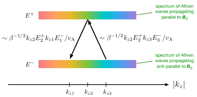
Figure 1: Physical interpretation of the wave kinetic equation for parametric decay when slow waves are strongly damped (Equation (11)). The mathematical expressions next to the arrows represent the contributions to $\partial E^{+}(k_{z2})/\partial t$ from the parametric decay of AWs at $k_{z3}$, which acts to increase $E^{+}(k_{z2})$, and the parametric decay of AWs at $k_{z2}$, which acts to decrease $E^{+}(k_{z2})$. In these expressions, $E^{+}_{2}=E^{+}(k_{z2})$, $E^{-}_{1}=E^{-}(k_{z1})$, and $E^{-}_{3}=E^{-}(k_{z3})$.

2.1 Physical Interpretation of the Wave Kinetic Equation

Figure 1 offers a way of understanding Equation (11). The horizontal color bars in this figure represent the spectra of outward-propagating and inward-propagating AWs, with red representing longer-wavelength waves and violet representing shorter-wavelength waves. AWs propagating in the $-\bm{B}_{0}$ direction at $|k_{z}|=k_{z3}$ decay into slow waves propagating anti-parallel to $\bm{B}_{0}$ at $|k_{z}|\simeq 2k_{z3}$ and AWs propagating parallel to $\bm{B}_{0}$ at $|k_{z}|=k_{z2}$. AWs propagating parallel to $\bm{B}_{0}$ at $|k_{z}|=k_{z2}$ decay into slow waves propagating parallel to $\bm{B}_{0}$ at $|k_{z}|\simeq 2k_{z2}$ and AWs propagating anti-parallel to $\bm{B}_{0}$ at $|k_{z}|=k_{z1}$. Equation (11) is approximately equivalent to the statement that the rate at which $E_{2}^{+}=E^{+}(k_{z2})$ increases via the decay of AWs at $|k_{z}|=k_{z3}$ is

$$R_{3\rightarrow 2}\sim\frac{k_{z2}E^{+}_{2}k_{z3}E^{-}_{3}}{\beta^{1/2}v_{\rm A}},$$ (13)

where $E^{-}_{3}=E^{-}(k_{z3})$, while the rate at which $E_{2}^{+}$ decreases via the decay of AWs at $|k_{z}|=k_{z2}$ is

$$R_{2\rightarrow 1}\sim\frac{k_{z2}E^{+}_{2}k_{z1}E^{-}_{1}}{\beta^{1/2}v_{\rm A}},$$ (14)

where $E^{-}_{1}=E^{-}(k_{z1})$. The time derivative of $E_{2}^{+}$ is $R_{3\rightarrow 2}-R_{2\rightarrow 1}$, or

$$\frac{\partial E^{+}_{2}}{\partial t}\sim\frac{k_{z2}E^{+}_{2}(k_{z3}E^{-}_{3}-k_{z1}E^{-}_{1})}{\beta^{1/2}v_{\rm A}}.$$ (15)

Equation (8) implies that $k_{z3}-k_{z1}\sim k_{z2}c_{\rm s}/v_{\rm A}\sim\beta^{1/2}k_{z2}$. A Taylor expansion of $k_{z3}E^{-}_{3}$ and $k_{z1}E^{-}_{1}$ about $k_{z2}$ in Equation (15) thus allows this equation to be rewritten as

$$\frac{\partial E^{+}_{2}}{\partial t}\sim\frac{k_{z2}^{2}E^{+}_{2}}{v_{\rm A}}\frac{\partial}{\partial k_{z}}\left(k_{z}E^{-})\right|_{k_{z}=k_{z2}},$$ (16)

which is the same as Equation (11) to within a factor of order unity.

To be clear, no independent derivation is being presented for Equations (13) and (14). The foregoing discussion merely points out that Equations (13) and (14) are equivalent (up to a factor of order unity) to Equation (11), which is derived on the basis of weak turbulence theory. It is worth pointing out, however, that several features of Equations (13) and (14) make sense on a qualitative level. If either $E^{+}=0$ or $E^{-}=0$, then $R_{3\rightarrow 2}=R_{2\rightarrow 1}=0$, because the parametric instability is a stimulated decay, which ceases if initially all the AWs travel in the same direction. For fixed $E^{+}$ and $E^{-}$, $R_{3\rightarrow 2}$ and $R_{2\rightarrow 1}$ vanish as $v_{\rm A}\rightarrow\infty$, since the fractional nonlinearities vanish in this limit. Also, $R_{3\rightarrow 2}$ and $R_{2\rightarrow 1}$ are proportional to $\beta^{-1/2}$ (when $S^{\pm}_{k}$ is negligibly small, as assumed) because the parametric-decay contribution to $\partial A_{k}^{\pm}/\partial t$ is an integral (over $\bm{p}$ and $\bm{q}$) of third-order correlation functions such as $\langle\delta\bm{v}_{k}\cdot\delta\bm{B}_{q}\delta n_{p}\rangle$, where $\delta\bm{v}_{k}$ and $\delta\bm{B}_{q}$ are the velocity and magnetic-field fluctuations associated with AWs at wave vectors $\bm{k}$ and $\bm{q}$, and $\delta n_{p}$ is the density fluctuation associated with the slow waves at wave vector $\bm{p}$ that are driven by the beating of the AWs at wave vectors $\bm{k}$ and $\bm{q}$. For fixed AW amplitudes and fixed $B_{0}$ and $v_{\rm A}$, this driven density fluctuation is proportional to $\beta^{-1/2}$, because as $\beta$ decreases the thermal pressure is less able to resist the compression along $\bm{B}_{0}$ resulting from the Lorentz force that arises from the beating of the AWs.

3 Linear Growth of the Parametric Instability

In the linear regime of the parametric instability, the spectrum of AWs propagating in one direction, say $E^{+}$, is taken to be fixed, and $E^{-}\ll E^{+}$. Equation (11) then implies that $E^{-}$ increases exponentially in time with growth rate

$$\gamma^{-}=\frac{\pi k_{z}^{2}}{v_{\rm A}}\frac{\partial}{\partial k_{z}}\left(k_{z}E^{+}\right).$$ (17)

Equation (17) is equivalent to Equation (18) of Cohen & Dewar (1974) given the different normalizations of the AW power spectra in the two equations. For example, Equation (12) implies that $\int_{0}^{\infty}E^{+}dk_{z}=(1/2)\int_{-\infty}^{\infty}E^{+}dk_{z}=\langle|\delta\bm{B}|^{2}\rangle/4\pi\rho$ when $E^{-}\ll E^{+}$, which can be compared with the un-numbered but displayed equation under Equation (9) of Cohen & Dewar (1974). As in the present paper, Cohen & Dewar (1974) assumed that slow waves are strongly damped and that the AWs satisfy the random-phase approximation. The present paper builds upon the results of Cohen & Dewar (1974) by investigating the coupled nonlinear evolution of $E^{+}$ and $E^{-}$. Also, whereas Cohen & Dewar (1974) took the wave vectors to be parallel or anti-parallel to $\bm{B}_{0}$, the derivation of Equation (11) in the present paper allows for obliquely propagating waves.

4 Conservation of Wave Quanta and Inverse Cascade

To simplify the presentation, it is assumed that

$$k_{z}>0.$$ (18)

No generality is lost, because $E^{\pm}$ is an even function of $k_{z}$, and thus it is sufficient to solve for the spectra at positive $k_{z}$ values. Equation (11) can be rewritten as the two equations

$$\frac{\partial N}{\partial t}+\frac{\partial\Gamma}{\partial k_{z}}=0$$ (19)

and

$$\frac{\partial\Gamma}{\partial t}=\pi\hbar k_{z}^{2}\Gamma\frac{\partial}{\partial k_{z}}\left(k_{z}^{2}N\right),$$ (20)

where

$$N=\frac{E^{+}+E^{-}}{\hbar k_{z}v_{\rm A}}$$ (21)

is the number of wave quanta per unit $k_{z}$ per unit mass and

$$\Gamma=-\frac{\pi k_{z}^{2}E^{+}E^{-}}{\hbar v_{\rm A}^{2}}$$ (22)

is the flux of wave quanta in $k_{z}$-space. Equation (19) implies that the number of wave quanta per unit mass,

$$N_{\rm tot}=\int_{-\infty}^{\infty}Ndk_{z},$$ (23)

is conserved. The fact that $\Gamma$ is negative indicates that there is an inverse cascade of wave quanta from large $k_{z}$ to small $k_{z}$ (c.f. Terasawa et al., 1986). The wavenumber drift velocity of the wave quanta,

$$\left\langle\frac{dk_{z}}{dt}\right\rangle\equiv\frac{\Gamma}{N}=-\frac{\pi k_{z}^{3}}{v_{\rm A}}\left(\frac{1}{E^{+}}+\frac{1}{E^{-}}\right)^{-1},$$ (24)

is determined primarily by the smaller of $E^{+}$ and $E^{-}$.

5 Exact Solutions to the Wave Kinetic Equations

In this section, several exact solutions to Equation (11) are presented under the assumption that $k_{z}>0$. The spectra at negative $k_{z}$ follow from the relation $E^{\pm}(-k_{z},t)=E^{\pm}(k_{z},t)$.

5.1 Decaying, Balanced Turbulence

One family of exact solutions to Equation (11) follows from setting

$$E^{\pm}(k_{z},t)=f^{\pm}(k_{z},t)H\big{(}k_{z}-b(t)\big{)}$$ (25)

in Equation (11), where

$$H(x)=\left\{\begin{array}[]{ll}0&\mbox{ if $x<0$}\\ 1&\mbox{ if $x\geq 0$}\end{array}\right.$$ (26)

is the Heaviside function. When Equation (25) is substituted into Equation (11), each side of Equation (11) becomes the sum of terms proportional to $\delta(k_{z}-b)$ and terms that contain no delta function. By separately equating the two groups of terms, one can show that Equation (25) is a solution to Equation (11) if

$$\frac{\partial}{\partial t}f^{\pm}(k_{z},t)=\frac{\pi}{v_{\rm A}}k_{z}^{2}f^{\pm}(k_{z},t)\frac{\partial}{\partial k_{z}}\left[k_{z}f^{\mp}(k_{z},t)\right]$$ (27)

and

$$\frac{1}{b^{3}}\frac{db}{dt}=-\frac{\pi f^{+}(b,t)}{2v_{\rm A}}=-\frac{\pi f^{-}(b,t)}{2v_{\rm A}}.$$ (28)

Equation (28) makes use of the relation $[H(x)]^{2}=H(x)$ and its derivative, $2H(x)\delta(x)=\delta(x)$. In Appendix A it is shown that Equation (28) can be recovered by adding a small amount of nonlinear diffusion to Equation (11) and replacing the discontinuous jump in the spectrum at $k_{z}=b(t)$ with a boundary layer. Equation (28) implies that, for solutions of the form given in Equation (25), the mean-square amplitudes of forward and backward-propagating AWs must be equal just above the break wavenumber $b$. An exact solution to Equations (27) and (28) corresponding to decaying turbulence is

$$f^{+}(k_{z},t)=f^{-}(k_{z},t)=\frac{a(t)}{k_{z}^{2}},$$ (29)

$$a(t)=a_{0}\left(1+\frac{\pi a_{0}t}{v_{\rm A}}\right)^{-1},$$ (30)

and

$$b(t)=b_{0}\left(1+\frac{\pi a_{0}t}{v_{\rm A}}\right)^{-1/2},$$ (31)

where $a_{0}$ and $b_{0}$ are the values of $a$ and $b$ at $t=0$.

This solution can be further truncated at large $k_{z}$ by setting

$$E^{+}(k_{z},t)=E^{-}(k_{z},t)=\frac{a(t)H(k_{z}-b(t))H(q(t)-k_{z})}{k_{z}^{2}}$$ (32)

with

$$q(t)=q_{0}\left(1+\frac{\pi a_{0}t}{v_{\rm A}}\right)^{-1/2},$$ (33)

where $q_{0}$ is the value of $q$ at $t=0$, which is taken to exceed $b_{0}$. Equations (29) through (33) can be recovered numerically by solving Equation (11) for freely decaying AWs. Whether the spectra satisfy Equations (25) and (29) through (31) or, alternatively, Equations (30) through (33), the number of wave quanta $N_{\rm tot}$ defined in Equation (23) is finite and independent of time.

5.2 Forced, Balanced Turbulence

An exact solution to Equations (27) and (28) corresponding to forced turbulence is

$$f^{+}(k_{z},t)=f^{-}(k_{z},t)=\frac{c}{k_{z}}$$ (34)

and

$$b(t)=\left(\frac{\pi ct}{2v_{\rm A}}+\frac{1}{b_{0}}\right)^{-1},$$ (35)

where $c$ is a constant and $b_{0}$ is the value of $b$ at $t=0$. In this solution, the number of wave quanta $N_{\rm tot}$ is not constant, because there is a nonzero influx of wave quanta from infinity. A version of this solution can be realized in a numerical solution of Equation (11) by holding $E^{\pm}$ fixed at some wavenumber $k_{\rm f}$, which mimics the effects of energy input from external forcing. In this case, the numerical solution at $k_{z}<k_{\rm f}$ is described by Equations (25), (34), and (35), with $b(t)<k_{\rm f}$.

The solution in Equations (34) and (35) can be truncated at large $k_{z}$ in a manner analogous to Equation (32), but with $q=[(\pi ct/2v_{\rm A})+(1/q_{0})]^{-1}$, where $q_{0}$ is the value of $q$ at $t=0$. In this solution, $N_{\rm tot}$ is independent of time. Numerical solutions of Equation (11) show, however, that this solution is unstable. If the spectra initially satisfy $E^{\pm}=(c/k_{z})H(k_{z}-b)H(q-k_{z})$, then they evolve towards the solution described by Equations (29) through (33).

5.3 Exact Solutions Extending over All $k_{z}$

In addition to the truncated solutions described in Sections 5.1 and 5.2, Equation (11) possesses several exact solutions that extend over all $k_{z}$. These solutions are unphysical, because they correspond to infinite AW energy and neglect dissipation (which becomes important at sufficiently large $k_{z}$) and finite system size (which becomes important at sufficiently small $k_{z}$). However, they illustrate several features of the nonlinear evolution of the parametric instability, which are summarized at the end of this section.

The simplest solution to Equation (11) spanning all $k_{z}$ is

$$E^{\pm}(k_{z},t)=\frac{c^{\pm}}{k_{z}},$$ (36)

where $c^{\pm}$ is a constant. It follows from Equation (22) that Equation (36) corresponds to a constant flux of AW quanta to smaller $k_{z}$. In contrast to the truncated $E^{\pm}\propto k_{z}^{-1}$ forced-turbulence solution in Section 5.2, $E^{+}$ and $E^{-}$ need not be equal in Equation (36).

A second, non-truncated, exact solution to Equation (11) is given by

$$E^{\pm}(k_{z},t)=\frac{a^{\pm}(t)}{k_{z}^{2}}$$ (37)

and

$$a^{\pm}(t)=\frac{a_{0}^{\pm}(a_{0}^{\pm}-a_{0}^{\mp})}{a_{0}^{\pm}-a_{0}^{\mp}e^{-\pi(a_{0}^{\pm}-a_{0}^{\mp})t/v_{\rm A}}},$$ (38)

where $a_{0}^{+}$ and $a_{0}^{-}$ are the initial values of $a^{+}$ and $a^{-}$. In this solution,

$$a^{+}(t)-a^{-}(t)=a_{0}^{+}-a_{0}^{-}.$$ (39)

If $a^{+}_{0}>a^{-}_{0}$, then $E^{-}$ decays faster than $E^{+}$, and, after a long time has passed, $E^{-}$ decays to zero while $a^{+}$ decays to the value $a^{+}_{0}-a^{-}_{0}$. Conversely, if $a^{-}_{0}>a_{0}^{+}$, then $E^{+}$ decays faster than $E^{-}$, and the turbulence decays to a state in which $E^{+}=0$. In the limit that $a_{0}^{+}\rightarrow a_{0}^{-}$,

$$a^{\pm}(t)\rightarrow a_{0}\left(1+\frac{\pi a_{0}t}{v_{\rm A}}\right)^{-1},$$ (40)

where $a_{0}=a^{+}_{0}=a^{-}_{0}$. Equations (37) and (40) are a non-truncated version of the decaying-turbulence solution presented in Section 5.1.

Equations (36) and (37) can be combined into a more general class of solution,

$$E^{\pm}(k_{z},t)=a^{\pm}(t)\left(\frac{1}{k_{z}^{2}}+\frac{d^{\pm}}{k_{z}}\right),$$ (41)

where $d^{+}$ and $d^{-}$ are constants and $a^{\pm}(t)$ is given by Equation (38). Another type of solution combining $k_{z}^{-1}$ and $k_{z}^{-2}$ scalings is

$$E^{+}(k_{z},t) = \frac{c_{0}e^{-\pi c_{2}t/v_{\rm A}}}{k_{z}},$$ (42)

$$E^{-}(k_{z},t) = \frac{c_{1}}{k_{z}}+\frac{c_{2}}{k_{z}^{2}},$$ (43)

where $c_{0}$, $c_{1}$, and $c_{2}$ are constants.

The exact solutions presented in this section illustrate three properties of the nonlinear evolution of the parametric instability at low $\beta$ when slow waves are strongly damped. First, when $E^{\pm}\propto k_{z}^{-1}$, $\partial E^{\mp}/\partial t$ vanishes. Second, if $E^{\pm}\propto k_{z}^{-2}$, then $(\partial/\partial t)\ln E^{\mp}$ is negative and independent of $k_{z}$, and $E^{\mp}(k_{z},t)$ can be written as the product of a function of $k_{z}$ and a (decreasing) function of time. (More general principles describing the evolution of $E^{\pm}$ are summarized in Figure 3 and Equation (54).) Third, the parametric instability does not necessarily saturate with $E^{+}=E^{-}$. For example, in Equations (37) and (38), when $a_{0}^{+}\neq a_{0}^{-}$, the AWs decay to a maximally aligned state reminiscent of the final state of decaying cross-helical incompressible MHD turbulence (Dobrowolny et al., 1980).

6 Nonlinear Evolution of the Parametric Instability When Most of the AWs Initially Propagate in the Same Direction

This section describes a numerical solution to Equation (11) in which, initially,

$$E^{+}\gg E^{-}.$$ (44)

As in Section 5, $k_{z}$ is taken to be positive, and the spectra at negative $k_{z}$ can be inferred from the fact that $E^{\pm}(-k_{z})=E^{\pm}(k_{z})$. The spectra are advanced forward in time using a second-order Runge-Kutta algorithm on a logarithmic wavenumber grid consisting of 2000 grid points. To prevent the growth of numerical instabilities, a nonlinear diffusion term

$$D^{\pm}=\nu E^{\mp}k_{z}^{2}\frac{\partial^{2}}{\partial k_{z}^{2}}E^{\pm}$$ (45)

is added to the right-hand side of Equation (11), where $\nu$ is a constant. The value of $\nu$ is chosen as small as possible subject to the constraint that the diffusion term suppress instabilities at the grid scale.

To represent the solution in a way that can be readily compared with spacecraft measurements of solar-wind turbulence, the wavenumber spectra are converted into frequency spectra,

$$e^{\pm}(f,t)=\frac{2\pi E^{\pm}(k_{z},t)}{U},$$ (46)

where $U$ is the solar-wind velocity, and

$$f=\frac{k_{z}U}{2\pi}$$ (47)

is the frequency in the spacecraft frame that, according to Taylor’s (1938) hypothesis, corresponds to wavenumber $k_{z}$ when the background magnetic field is aligned with the nearly radial solar-wind velocity. The Alfvén speed is taken to be the approximate average of the observed values of $v_{\rm A}$ in three fast-solar-wind streams at $r=0.3\mbox{ AU}$ (see Table 1 of Marsch et al. (1982) and Table 1a of Marsch & Tu (1990)),

$$v_{\rm A}=150\mbox{ km/s}.$$ (48)

In order to compare directly with Figure 2-2c of Tu & Marsch (1995), the solar-wind velocity is taken to be

$$U=733\mbox{ km/s}.$$ (49)

The power spectra are initialized to the values

$$e^{+}(f,t=0)=\frac{\sigma^{+}(f/f_{0})^{-0.5}}{1+(f/f_{0})^{1.5}}$$ (50)

and

$$e^{-}(f,t=0)=\sigma^{-},$$ (51)

where $\sigma^{+}$, $\sigma^{-}$, and $f_{0}$ are constants. The values of $f_{0}$ and the corresponding wavenumber $k_{z0}$ are chosen so that

$$f_{0}=\frac{k_{z0}U}{2\pi}=10^{-2}\mbox{ Hz},$$ (52)

consistent with the arguments of van Ballegooijen & Asgari-Targhi (2016) about the dominant frequency of AW launching by the Sun. The minimum and maximum wavenumbers of the numerical domain are chosen so that $k_{z\rm max}=10^{3}k_{z0}=10^{7}k_{z\rm min}$. The motivation for the scaling $e^{+}(f,t=0)\propto f^{-0.5}$ at small $f$ is the similar scaling observed by Tu & Marsch (1995) in the aforementioned fast-solar-wind stream at $10^{-5}\mbox{ Hz}<f<10^{-4}\mbox{ Hz}$. The numerical results shown below suggest that the parametric instability has little effect on $e^{+}$ at these frequencies at $r=0.3\mbox{ AU}$. The observed $f^{-0.5}$ scaling in this frequency range is thus presumably inherited directly from the spectrum of AWs launched by the Sun. Like the scaling $e^{+}\propto f^{-0.5}$, the value of $\sigma^{+}$ is chosen to match the observed spectrum of outward-propagating AWs at 0.3 AU at small $f$. The reason for the $f^{-2}$ scaling in $e^{+}$ at large $f$ is that a (parallel) $k_{z}^{-2}$ spectrum is observed in the solar wind (Horbury et al., 2008; Podesta, 2009; Forman et al., 2011) and predicted by the theory of critically balanced MHD turbulence (see, e.g., Goldreich & Sridhar, 1995; Mallet et al., 2015). The value of $\sigma^{-}$ is set equal to a minuscule value ($10^{-12}\sigma^{+}$), so that the only source of dynamically important, inward-propagating AWs is the parametric decay of outward-propagating AWs.

Figure 2 summarizes the results of the calculation. Between $t=0$ and $t=4\mbox{ hr}$, $e^{+}$ changes little while $e^{-}$ grows rapidly between roughly 2 and 5 mHz, where the growth rate $\gamma^{-}$ given in Equation (17) peaks. Between $t=4\mbox{ hr}$ and $t=8\mbox{ hr}$, $e^{+}$ develops a broad $\sim 1/f$ scaling between $f=3\times 10^{-4}\mbox{ Hz}$ and $f=3\times 10^{-2}\mbox{ Hz}$, which shuts off the growth of $e^{-}$ at these frequencies. At the same time, $e^{-}$ acquires an $\sim f^{-2}$ scaling over much of this same frequency range. Between $t=8\mbox{ hr}$ and $t=16\mbox{ hr}$, the low-frequency limit of the $1/f$ range of $e^{+}$ decreases to $\sim 10^{-4}\mbox{ Hz}$, and the high-frequency limit of the $1/f$ range of $e^{+}$ increases to $\sim 0.1\mbox{ Hz}$.

Figure 2: Solid lines show the AW power spectra in a numerical solution of Equation (11) with plasma parameters and turbulence parameters chosen to model conditions in the fast solar wind at a heliocentric distance of 0.3 AU. The wavenumber spectra $E^{\pm}(k_{z})$ appearing in Equation (11) have been converted, using Equations (46) and (47), into the frequency spectra $e^{\pm}(f)$. The dotted lines in the upper left corners of each plot show the evolutionary tracks of the values of $e^{+}$ and $e^{-}$ at the low-frequency end of the frequency range in which $e^{+}\propto f^{-1}$ in the approximate analytic solution to Equation (11) presented in Appendix B.

The dotted lines in the upper left corner of each panel in Figure 2 show the tracks followed by the values of $e^{+}$ and $e^{-}$ at the low-frequency end of the frequency range in which $e^{+}\propto f^{-1}$ in the approximate analytic solution to Equation (11) that is described in Appendix B. In this solution, $E^{+}$ and $E^{-}$ are expanded in negative powers of $k_{z}$ at wavenumbers exceeding a time-dependent break wavenumber $b(t)$. Below this wavenumber, $E^{-}=0$ and $E^{+}=\eta k_{z}^{p}$, where $\eta$ and $p$ are constants, and $-1<p<1$. At $k_{z}>b$, the dominant term in the expansion of $E^{+}$ ($E^{-}$) scales like $k_{z}^{-1}$ ($k_{z}^{-2}$), and the ratios of $E^{+}(b_{+})$ to $\eta b_{+}^{p}$ and $E^{+}(b_{+})$ to $E^{-}(b_{+})$ are fixed functions of $p$, where $b_{+}$ is a wavenumber infinitesimally larger than $b$. For $p=-0.5$, $E^{+}(b_{+})/\eta b_{+}^{p}=5/3$ and $E^{+}(b_{+})/E^{-}(b_{+})=10$, in approximate agreement with the numerical results (see also the right panel of Figure 4).

6.1 Heuristic Explanation of the $e^{+}\propto f^{-1}$ and $e^{-}\propto f^{-2}$ Scalings

In order to understand the time evolution illustrated in Figure 2, it is instructive to first consider the case in which

$$E^{\pm}=c^{\pm}k_{z}^{\alpha^{\pm}}$$ (53)

within some interval $(k_{z1},k_{z2})$, where $c^{\pm}$ and $\alpha^{\pm}$ are constants. Equation (11) implies that, within this interval,

$$\frac{\partial}{\partial t}\ln E^{\pm}=\frac{\pi c^{\mp}}{v_{\rm A}}\left(1+\alpha^{\mp}\right)k_{z}^{\alpha^{\mp}+2}.$$ (54)

If $\alpha^{\mp}>-1$, then $\ln E^{\pm}$ grows at a rate that increases with $k_{z}$, causing $E^{\pm}$ to increase and “harden,” in the sense that the best-fit value of $\alpha^{\pm}$ within the interval $(k_{z1},k_{z2})$ increases. If $\alpha^{\mp}=-1$, then $E^{\pm}$ does not change. If $-2<\alpha^{\mp}<-1$, then $\ln E^{\pm}$ decreases at a rate that increases with $k_{z}$, which causes the best-fit value of $\alpha^{\pm}$ within the interval $(k_{z1},k_{z2})$ to decrease. If $\alpha^{\mp}=-2$, then $\ln E^{\pm}$ decreases at the same rate at all $k_{z}$, and $\alpha^{\pm}$ remains unchanged. Finally, if $\alpha^{\mp}<2$, then $E^{\pm}$ decreases at a rate that decreases with $k_{z}$, which causes the best-fit value of $\alpha^{\pm}$ in the interval $(k_{z1},k_{z2})$ to increase. These rules are summarized in Figure 3 and apply to $e^{\pm}\propto f^{\alpha^{\pm}}$ as well as $E^{\pm}\propto k_{z}^{\alpha^{\pm}}$.

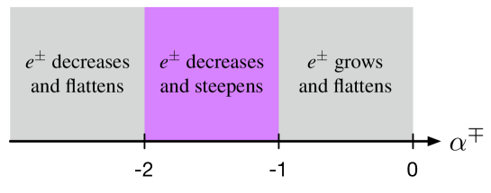
Figure 3: In this figure, it is assumed that the frequency spectra are initially power laws of the form $e^{\pm}\propto f^{\alpha^{\pm}}$, and that $\alpha^{+}$ and $\alpha^{-}$ are both negative. According to Equation (54), parametric decay alters both the amplitude and slope of $e^{\pm}$ in the manner shown. For example, if $e^{-}\propto f^{-1.5}$, then $E^{+}\propto k_{z}^{-1.5}$, and Equation (54) implies that $E^{+}$ decreases at a rate that increases with $k_{z}$. This in turn implies that $e^{+}$ decreases at a rate that increases with $f$, so that $e^{+}$ steepens.

Returning to Figure 2, in the early stages of the numerical calculation, $e^{-}$ grows most rapidly at those frequencies at which $\gamma^{-}$ in Equation (17) is largest — namely, the high-$f$ end of the $f^{-0.5}$ range of $e^{+}$. By the time $e^{-}$ reaches a sufficient amplitude that $e^{+}$ and $e^{-}$ evolve on the same timescale, $e^{-}$ develops a peaked frequency profile extending from some frequency $f=f_{\rm low}$ to some larger frequency $f=f_{\rm high}$, as illustrated in the upper-right panel of Figure 2. Near $f_{\rm low}$, $de^{-}/df>0$ (i.e., $\alpha^{-}>0$), which causes $e^{+}$ to grow. Near $f_{\rm high}$, $\alpha^{-}<-1$, which causes $e^{+}$ to decrease. Thus, $e^{+}$ steepens across the interval $(f_{\rm low},f_{\rm high})$ until it attains a $1/f$ scaling, at which point $e^{-}$ stops growing between $f_{\rm low}$ and $f_{\rm high}$. However, at frequencies just below $f_{\rm low}$, $e^{+}$ and $e^{-}$ both continue to grow, causing $f_{\rm low}$ to decrease. At the same time, $e^{+}$ continues to decrease at larger $f$ where $\alpha^{-}<-1$. Together, the growth of $e^{+}$ just below $f_{\rm low}$ and the damping of $e^{+}$ at larger $f$ cause the $f^{-1}$ range of $e^{+}$ to broaden in both directions, i.e., towards both smaller and larger frequencies.

The unique scaling of $e^{-}$ consistent with an $e^{+}$ spectrum $\propto f^{-1}$ that is a decreasing function of time is $e^{-}\propto f^{-2}$. Moreover, the scalings $e^{+}\sim f^{-1}$ and $e^{-}\sim f^{-2}$ are, in a sense, stable, as can be inferred from Figure 3. For example, if $\alpha^{-}$ increases from $-2$ to a slightly larger value, then $e^{+}$ decreases at a rate that increases with $f$, causing $\alpha^{+}$ to decrease to a value slightly below $-1$. This causes $e^{-}$ to decrease at a rate that increases with $f$, thereby causing $\alpha^{-}$ to decrease back towards $-2$. A similar “spectral restoring force” arises for any other small perturbation to the values $\alpha^{+}=-1$ and $\alpha^{-}=-2$.

It is worth emphasizing, in this context, that the analytic solution presented in Appendix B is approximate rather than exact. As the spectral break frequency decreases past some fixed frequency $f_{3}$, the values of $e^{+}$ and $e^{-}$ at $f_{3}$ suddenly jump, but they do not jump to the precise values needed to extend the $e^{+}\sim f^{-1}$ and $e^{-}\sim f^{-2}$ scalings to smaller $f$. Instead, the spectra need further “correcting” after the break frequency has swept past in order to maintain the scalings $e^{+}\sim f^{-1}$ and $e^{-}\sim f^{-2}$ in an approximate way. Also, the decrease in $e^{-}$ that occurs after $t=4\mbox{ hr}$ is a consequence of the sub-dominant $f^{-2}$ component of $e^{+}$. This component of $e^{+}$ becomes increasingly prominent near the break frequency as time progresses, leading to the pronounced curvature in the plot of $e^{+}$ near $f=10^{-4}\mbox{ Hz}$ in the right panel of Figure 4.

Figure 4: The left panel and middle panel of this figure reproduce the $t=4\mbox{ hr}$ and $t=8\mbox{ hr}$ panels of Figure 2 but with the axis ranges used in Figure 2-2c of Tu & Marsch (1995). The right panel is from a later time ($t=32\mbox{ hr}$) in the same numerical solution.

6.2 Comparison with Helios Measurements

In the (average) plasma rest frame, the equations of incompressible MHD can be written in the form

$$\frac{\partial\bm{z}^{\pm}}{\partial t}+(\bm{z}^{\mp}\pm\bm{v}_{\rm A})\cdot\nabla\bm{z}^{\pm}=-\nabla\Pi,$$ (55)

where $\bm{z}^{\pm}=\delta\bm{v}\mp\delta\bm{B}/\sqrt{4\pi\rho}$ are the Elsasser variables, $\delta\bm{v}$ and $\delta\bm{B}$ are the velocity and magnetic-field fluctuations, $\rho$ is the mass density, $\bm{v}_{\rm A}=\bm{B}_{0}/\sqrt{4\pi\rho}$ is the Alfvén velocity, and $\Pi$ is the total pressure divided by $\rho$ (Elsasser, 1950). Although the solar wind is compressible, Equation (55) provides a reasonable approximation for the non-compressive, AW-like component of solar-wind turbulence. As Equation (55) shows, the advection velocity of a $\bm{z}^{\pm}$ fluctuation is $\bm{z}^{\mp}\pm\bm{v}_{\rm A}$. This implies, as shown by Maron & Goldreich (2001), that $\bm{z}^{\pm}$ fluctuations propagate along magnetic field lines perturbed by $\bm{z}^{\mp}$. As a consequence, in the solar wind, when the rms magnetic-field fluctuation $\delta B_{\rm in}$ associated with inward-propagating AWs ($\bm{z}^{-}$) is much smaller than the background magnetic field $B_{0}$, the outward-propagating AWs ($\bm{z}^{+}$) propagate to a good approximation along the direction of $\bm{B}_{0}$. This is true even if the rms magnetic-field fluctuation $\delta B_{\rm out}$ associated with $\bm{z}^{+}$ is comparable to $B_{0}$. In the fast solar wind at $r<0.3\mbox{ AU}$, the (fractional) cross helicity is high (i.e., $E^{+}\gg E^{-}$), and $\delta B_{\rm in}$ is indeed small compared to $B_{0}$ (Bavassano et al., 2000; Cranmer & van Ballegooijen, 2005). Moreover, the background magnetic field at $r=0.3\mbox{ AU}$ is nearly in the radial direction, because the Parker-spiral magnetic field begins to deviate appreciably from the radial direction only at larger $r$ in the fast wind (Verscharen et al., 2015). Hence, in high-cross-helicity fast-wind streams at $r=0.3\mbox{ AU}$, the function $e^{+}$ defined by Equations (46) and (47) corresponds to a good approximation to the frequency spectrum of outward-propagating AWs observed by a spacecraft in the solar wind. It is not clear, however, how well $e^{-}$ corresponds to the observed spectrum of inward-propagating AWs, because the inward-propagating AWs follow field lines perturbed by the outward-propagating AWs, which can be inclined relative to the radial direction by a substantial angle.

Figure 4 reproduces the $t=4\mbox{ hr}$ and $t=8\mbox{ hr}$ panels of Figure 2, but with the same axis ranges as those in Figure 2-2c of Tu & Marsch (1995) to facilitate comparison. Figure 4 also includes a third panel that shows the spectra at $t=32\mbox{ hr}$. The $e^{+}$ spectrum in the $t=8\mbox{ hr}$ panel of Figure 2 shares a number of properties with the $e^{+}$ spectrum in Figure 2-2c of Tu & Marsch (1995), in addition to the $f^{-0.5}$ scaling at small $f$ that was built in to the numerical calculation as an initial condition. In particular, $e^{+}\gg e^{-}$ at all frequencies, $e^{+}\sim f^{-1}$ at $f\gtrsim 3\times 10^{-4}\mbox{ Hz}$, and there is a bump in the $e^{+}$ spectrum at the transition between the $f^{-0.5}$ and $f^{-1}$ scaling ranges of $e^{+}$.

Although this comparison is suggestive, it is not entirely clear how to map time in the numerical calculation to heliocentric distance in the solar wind, because the plasma parameters in the numerical calculation are independent of position and time, whereas they depend strongly upon heliocentric distance in the solar wind. For example, the turbulence is weaker (in the sense of smaller $\delta v_{0}/v_{\rm A}$) the closer one gets to the Sun. (See also the discussion following Equation (65).) Also, the choice of initial conditions in the numerical calculation artificially prolongs the linear stage of evolution, since in the solar wind there are sources of inward-propagating waves other than parametric instability, such as non-WKB reflection (Heinemann & Olbert, 1980; Velli, 1993). Nevertheless, as a baseline for comparison, the travel time of an outward-propagating AW from the photosphere to $0.3\mbox{ AU}$ in the fast-solar-wind model developed by Chandran & Hollweg (2009) is approximately 12 hr.

7 Discussion of Approximations and Relevance to the Solar Wind

This section critically assesses the assumptions underlying the results in Sections 2 through 6 and the degree to which these assumptions apply to the fast solar wind between $r=10R_{\odot}$ (the approximate perihelion of the Parker Solar Probe) and $r=0.3\mbox{ AU}$.

7.1 The Weak Turbulence Approximation

A central assumption of the analysis is the weak-turbulence criterion in Equation (1). Since $E^{+}$ and $E^{-}$ differ in the solar wind, Equation (1) is really two conditions,

$$\omega_{\rm nl}^{\pm}\ll|k_{z}|v_{\rm A},$$ (56)

where $\omega_{\rm nl}^{+}$ ($\omega_{\rm nl}^{-}$) is the inverse of the timescale on which nonlinear interactions modify outward-propagating (inward-propagating) AWs. The contribution to $\omega_{\rm nl}^{\pm}$ from the parametric instability is

$$\omega_{\rm nl,PI}^{\pm}\sim\frac{1}{E^{\pm}}\left|\frac{\partial E^{\pm}}{\partial t}\right|\sim\frac{k_{z}^{2}E^{\mp}}{v_{\rm A}}.$$ (57)

The contribution to $\omega_{\rm nl}^{\pm}$ from one other type of nonlinear interaction is estimated in Section 7.3. The estimate of $\partial E^{\pm}/\partial t$ in Equation (57) follows from Equation (11) and setting $E^{\mp}\sim|k_{z}|^{\alpha^{\mp}}$ with $\alpha^{\mp}$ not very close to $-1$. A rough upper limit on $\omega_{\rm nl,PI}^{\pm}$ results from replacing $k_{z}E^{\mp}$ in Equation (57) with $(\delta v^{\mp})^{2}$, where $(\delta v^{+})^{2}$ is the mean-square velocity fluctuation associated with outward-propagating AWs, and $(\delta v^{-})^{2}$ is the mean-square velocity fluctuation associated with inward-propagating AWs. This leads to a rough upper limit on $\omega_{\rm nl,PI}^{\pm}$ because $(\delta v^{\pm})^{2}$ includes contributions from all wavenumbers and is much larger than the value of $k_{z}E^{\pm}$ at some $k_{z}$. Equation (56), with $\omega_{\rm nl}\sim\omega_{\rm nl,PI}$, is thus satisfied provided

$$(\delta v^{\mp})^{2}\ll v_{\rm A}^{2}.$$ (58)

Bavassano et al. (2000) analyzed Helios measurements of fluctuations in the fast solar wind at $r=0.4\mbox{ AU}$ and found that $(\delta v^{-})^{2}\ll(\delta v^{+})^{2}\simeq(60\mbox{ km/s})^{2}$. As mentioned above, the typical value of $v_{\rm A}$ in the fast solar wind at $r=0.3\mbox{ AU}$ is $\sim 150\mbox{ km/s}$ (Marsch et al., 1982; Marsch & Tu, 1990). Near $r=0.3\mbox{ AU}$, $B_{0}\sim 1/r^{2}$, $\rho\sim 1/r^{2}$, and $v_{\rm A}\sim 1/r$, and so the typical value of $v_{\rm A}$ in fast-solar-wind streams at $r=0.4\mbox{ AU}$ is $\sim 112.5\mbox{ km/s}$. These measurements indicate that

$$(\delta v^{-})^{2}\ll(\delta v^{+})^{2}\simeq 0.28v_{\rm A}^{2}$$ (59)

in the fast solar wind at $r=0.4\mbox{ AU}$. Since $\delta v^{\pm}/v_{\rm A}$ decreases as $r$ decreases below 0.4 AU (Cranmer & van Ballegooijen, 2005; Chandran & Hollweg, 2009), the condition $\omega_{\rm nl,PI}^{+}\ll|k_{z}|v_{\rm A}$ is well satisfied at $r<0.4\mbox{ AU}$, and the condition $\omega_{\rm nl,PI}^{-}\ll|k_{z}|v_{\rm A}$ is at least marginally satisfied at $r<0.4\mbox{ AU}$.

It is worth noting that weak turbulence theory fails when applied to resonant interactions between three AWs, because such interactions occur only when one of the AWs has zero frequency, violating the weak-turbulence ordering (Schekochihin et al., 2012; Meyrand et al., 2015). In contrast, the AW/slow-wave interactions in parametric decay do not involve a zero-frequency mode. Weak turbulence theory is thus in principle a better approximation for the nonlinear evolution of the parametric instability than for incompressible MHD turbulence.

7.2 The Low-$\beta$ Assumption

The assumption that $\beta\ll 1$ is not satisfied at $r\gtrsim 0.3\mbox{ AU}\simeq 65R_{\odot}$, where $\beta$ is typically $\sim 1$, but is reasonable at $r\lesssim 20R_{\odot}$ (Chandran et al., 2011). It is possible that the $\beta\ll 1$ theory presented here applies at least at a qualitative level provided $\beta$ is simply $\lesssim 1$, and indeed this possibility motivates the comparison of the present model with Helios observations. However, further work is needed to investigate how the results of this paper are modified as $\beta$ increases to values $\sim 1$.

7.3 Neglect of Other Types of Nonlinear Interactions

Another approximation in Sections 2 through 6 is the neglect of all nonlinear interactions besides parametric decay. One of the neglected interactions is the shearing of inward-propagating AWs by outward-propagating AWs, which makes a contribution to $\omega^{-}_{\rm nl}$ that depends on the perpendicular length scale of the AWs. At the perpendicular outer scale $L_{\perp}$ (the overall correlation length of the AWs measured perpendicular to $\bm{B}_{0}$), the contribution to $\omega^{-}_{\rm nl}$ from shearing is approximately

$$\omega_{\rm nl,\perp}^{-}\sim\frac{\chi\delta v^{+}}{L_{\perp}},$$ (60)

where

$$\chi=\frac{\delta v^{+}}{k_{z}L_{\perp}v_{\rm A}}$$ (61)

is the critical-balance parameter (Goldreich & Sridhar, 1995; Ng & Bhattacharjee, 1996; Lithwick et al., 2007). Equation (60) does not apply when $\chi$ is much larger than 1, but direct numerical simulations suggest that $\chi\lesssim 1$ at $r\gtrsim 10R_{\odot}$ for the bulk of the AW energy (J. Perez, private communication). Thus, at $r\gtrsim 10R_{\odot}$,

$$\frac{\omega_{\rm nl,PI}^{-}}{\omega_{\rm nl,\perp}^{-}}\simeq(k_{z}L_{\perp})^{2}.$$ (62)

As AWs propagate away from the Sun, they follow magnetic field lines, which leads to the approximate scaling $L_{\perp}\propto B_{0}^{-1/2}$. In the WKB limit, the AW frequency in the Sun’s frame $k_{z}(U+v_{\rm A})$ is independent of $r$. The scaling $k_{z}\sim 1/(U+v_{\rm A})$ thus serves as a rough approximation for outward-propagating AWs in the turbulent solar wind. At the coronal base (just above the transition region), where $k_{z}$ and $L_{\perp}$ have the values $k_{z\rm b}$ and $L_{\perp\rm b}$, the value of $k_{z\rm b}L_{\perp\rm b}$ for the energetically dominant AWs launched by the Sun can be estimated (in essence from the critical-balance condition) as $\delta v_{\rm b}^{+}/v_{\rm Ab}$, where $\delta v_{\rm b}^{+}$ and $v_{\rm Ab}$ are the values of $\delta v^{+}$ and $v_{\rm A}$ at the coronal base (Goldreich & Sridhar, 1995; van Ballegooijen & Asgari-Targhi, 2016). Together, these scalings lead to the estimate

$$k_{z}L_{\perp}\simeq\sqrt{\frac{B_{0\rm b}}{B_{0}}}\left(\frac{U_{\rm b}+v_{\rm Ab}}{U+v_{\rm A}}\right)\frac{\delta v^{+}_{\rm b}}{v_{\rm Ab}},$$ (63)

where $B_{0\rm b}$ and $U_{\rm b}$ are the values of the background magnetic field and solar-wind outflow velocity at the coronal base. Between $r=10R_{\odot}$ and $r=60R_{\odot}$, $B_{0\rm b}/B_{0}\simeq f_{\rm max}(r/R_{\odot})^{2}$, where $f_{\rm max}$ is the super-radial expansion factor (Kopp & Holzer, 1976). In the fast solar wind within this range of radii, $U+v_{\rm A}\simeq 700-800\mbox{ km/s}$, which is comparable to $U_{\rm b}+v_{\rm Ab}\simeq v_{\rm Ab}\simeq 10^{3}\mbox{ km/s}$. Equation (63) is thus approximately equivalent to

$$k_{z}L_{\perp}\simeq\sqrt{f_{\rm max}}\,\left(\frac{r}{R_{\odot}}\right)\left(\frac{\delta v_{\rm b}^{+}}{v_{\rm Ab}}\right)$$ (64)

for the energetically dominant fluctuations launched by the Sun. If we set $f_{\rm max}=9$, $\delta v_{\rm b}=30\mbox{ km/s}$, and $v_{\rm Ab}=900\mbox{ km/s}$, then Equation (64) becomes

$$k_{z}L_{\perp}\sim\frac{r}{10R_{\odot}}$$ (65)

for the energetically dominant AWs launched by the Sun. Equations (62) and (65) suggest that it is reasonable to neglect the shearing of inward-propagating AWs by outward-propagating AWs at $r\gtrsim 10R_{\odot}$. On the other hand, at smaller radii, shearing could suppress the growth of inward-propagating AWs that would otherwise result from the parametric instability. Also, the requirement that $k_{z}L_{\perp}>1$ in order for $\omega_{\rm nl,PI}^{-}$ to exceed $\omega_{\rm nl,\perp}^{-}$ could prevent the $f^{-1}$ range from spreading to frequencies below some minimum ($r$-dependent) value.

The other nonlinearities in the weak-turbulence wave kinetic equations that are neglected in this paper include interactions involving fast magnetosonic waves, the turbulent mixing of slow waves by AWs, phase mixing of AWs by slow waves, and the shearing of outward-propagating AWs by inward-propagating AWs (Chandran, 2008). In-situ measurements indicate that fast waves account for only a small fraction of the energy in compressive fluctuations at 1 AU (Yao et al., 2011; Howes et al., 2012; Klein et al., 2012). Also, fast waves propagating away from the Sun undergo almost complete reflection before they can escape into the corona (Hollweg, 1978). These findings suggest that nonlinear interactions involving fast waves have little effect upon the conclusions of this paper. The turbulent mixing of slow waves by AWs acts as an additional slow-wave damping mechanism and is thus unlikely to change the conclusions of this paper, which already assume strong slow-wave damping. Phase mixing of AWs by slow waves transports AW energy to larger $k_{\perp}$ at a rate that increases with $|k_{z}|$ (Chandran, 2008). Although the fractional density fluctuations between $r=10R_{\odot}$ and $r=0.3\mbox{ AU}$ are fairly small (see, e.g., Tu & Marsch, 1995; Hollweg et al., 2010), phase mixing could affect the parallel AW power spectra, and further work is needed to investigate this possibility. The shearing of outward-propagating AWs by inward-propagating AWs is enhanced by non-WKB reflection, which makes this shearing more coherent in time (Velli et al., 1989). The resulting nonlinear timescale for outward-propagating AWs is roughly $r/(U+v_{\rm A})$ (Chandran & Hollweg, 2009), where $U$ is the solar-wind outflow velocity. This timescale is comparable to the AW propagation time from the Sun to heliocentric distance $r$, and hence to the parametric-decay timescale at the small-$f$ end of the $1/f$ range of $e^{+}$. How this shearing modifies $E^{+}(k_{z})$, however, is not clear. For example, shearing by inward-propagating AWs may transport outward-propagating-AW energy to larger $k_{\perp}=\sqrt{k_{x}^{2}+k_{y}^{2}}$ at a rate that is independent of $|k_{z}|$, in which case this shearing would reduce $E^{+}(k_{z})$ by approximately the same factor at all $k_{z}$, leaving the functional form of $E^{+}(k_{z})$ unchanged.

7.4 Neglect of Spatial Inhomogeneity

In this paper, it is assumed that the background plasma is uniform and stationary. In the solar wind, however, as an AW propagates from the low corona to 0.3 AU, the properties of the ambient plasma seen by the AW change dramatically, with $\beta$ increasing from $\sim 10^{-2}$ to $\sim 1$ and $\delta v_{\rm rms}/v_{\rm A}$ increasing from $\sim 0.02$ to $\sim 0.5$ (Bavassano et al., 2000; Cranmer & van Ballegooijen, 2005; Chandran et al., 2011). Further work is needed to determine how this spatial inhomogeneity affects the nonlinear evolution of the parametric instability.

7.5 Approximate Treatment of Slow-Wave Damping

A key assumption in Sections 2 through 6 is that slow waves are strongly damped, and this damping is implemented by neglecting terms in the wave kinetic equations that are proportional to the slow-wave power spectrum $S^{\pm}_{k}$. There are two sources of error in this approach. First, damping could modify the polarization properties of slow waves, thereby altering the wave kinetic equations. Second, even if $S^{\pm}_{k}$ is much smaller than the AW power spectrum $A^{\pm}_{k}$, the neglected parametric-decay terms in the wave kinetic equations for AWs that are proportional to $S^{\pm}_{k}$ could still be important, because they contain a factor of $\beta^{-1}$, which is absent in the terms that are retained. This factor arises from the fact that the fractional density fluctuation of a slow wave is $\sim\beta^{-1/2}$ times larger than the fractional magnetic-field fluctuation of an AW with equal energy. These neglected terms act to equalize the 3D AW power spectra $A^{+}$ and $A^{-}$, and hence to equalize $E^{+}$ and $E^{-}$. If these neglected terms were in fact important, they could invalidate the solutions presented in Section 6, in which $E^{+}\gg E^{-}$. However, in situ observations indicate that $E^{+}\gg E^{-}$ in the fast solar wind at $r=0.3\mbox{ AU}$ (Marsch & Tu, 1990; Tu & Marsch, 1995), which suggests that the neglect of these terms is reasonable. Further work is needed to investigate these issues more carefully.

8 Conclusion

In this paper, weak turbulence theory is used to investigate the nonlinear evolution of the parametric instability in low-$\beta$ plasmas. The analysis starts from the wave kinetic equations describing the interactions between AWs and slow waves in weak compressible MHD turbulence. To account for the strong damping of slow waves in collisionless plasmas, terms containing the slow-wave energy density are dropped. The equations allow for all wave-vector directions, but are integrated over the wave-vector components perpendicular to the background magnetic field $\bm{B}_{0}$ ($k_{x}$ and $k_{y}$), which leads to equations for the 1D power spectra $E^{+}$ and $E^{-}$ that depend only on the parallel wavenumber $k_{z}$ and time. During parametric decay in a low-$\beta$ plasma, an AW decays into a slow wave propagating in the same direction and a counter-propagating AW with a frequency slightly smaller than the frequency of the initial AW. The total number of AW quanta is conserved, and the reduction in AW frequencies leads to an inverse cascade of AW quanta towards smaller $\omega$ and $k_{z}$. The energy of each AW quantum is $\hbar\omega$, and the decrease in $\omega$ during each decay corresponds to a decrease in the AW energy, which is compensated for by an increase in the slow-wave energy. The subsequent damping and dissipation of slow-wave energy results in plasma heating.

The main results of this paper concern the parametric decay of a population of AWs propagating in one direction, say parallel to $\bm{B}_{0}$, when the counter-propagating AWs start out with much smaller amplitudes. If the initial frequency spectrum $e^{+}$ of the parallel-propagating AWs has a peak frequency $f_{0}$ (at which $fe^{+}$ is maximized) and an “infrared” scaling $f^{p}$ at smaller $f$ with $-1<p<1$, then $e^{+}$ acquires a $1/f$ scaling throughout a range of frequencies that spreads out in both directions from $f_{0}$. At the same time, the anti-parallel-propagating AWs acquire a $1/f^{2}$ spectrum within this same frequency range. If the plasma parameters and infrared $e^{+}$ spectrum are chosen to match conditions in the fast solar wind at a heliocentric distance of 0.3 AU, and the AWs are allowed to evolve for a period of time that is roughly two-thirds of the AW travel time from the Sun to 0.3 AU, the resulting form of $e^{+}$ is similar to the form observed by the Helios spacecraft in the fast solar wind at 0.3 AU. Because the background plasma parameters are time-independent in the analysis of this paper but time-dependent in the plasma rest frame in the solar wind, it is not clear how to map the time variable in the present analysis to heliocentric distance. Nevertheless, the similarity between the spectra found in this paper and the spectra observed by Helios suggests that parametric decay plays an important role in shaping the AW spectra observed in the fast solar wind at 0.3 AU, at least for wave periods $\lesssim 1\mbox{ hr}$.

The frequency $f^{\ast}$ that dominates the AW energy is the maximum of $(fe^{+}+fe^{-})$. At the beginning of the numerical calculation presented in Section 6, $f^{\ast}$ is approximately $f_{0}=0.01\mbox{ Hz}$. At $t=8\mbox{ hr}$ in this numerical calculation, $f^{\ast}$ is the smallest frequency at which $e^{+}\sim f^{-1}$ and $e^{-}\sim f^{-2}$, which is $\sim 3\times 10^{-4}\mbox{ Hz}$. This decrease in $f^{\ast}$ is a consequence of the aforementioned inverse cascade, which transports AW quanta from the initial peak frequency to smaller frequencies. Inverse cascade offers a way to reconcile the observed dominance of AWs at hour-long timescales at 0.3 AU with arguments that the Sun launches most of its AW power at significantly shorter wave periods (Cranmer & van Ballegooijen, 2005; van Ballegooijen & Asgari-Targhi, 2016).

Further work is needed to relax some of the simplifying assumptions in this paper, including the low-$\beta$ approximation, the assumption of spatial homogeneity, the simplistic treatment of slow-wave damping, and the neglect of nonlinear interactions other than parametric decay. Further work is also needed to evaluate the relative contributions of parametric decay and other mechanisms to the generation of $1/f$ spectra in the solar wind. For example, Matthaeus & Goldstein (1986) argued that the $f^{-1}$ spectrum seen at $r=1\mbox{ AU}$ at $3\times 10^{-6}\mbox{ Hz}<f<8\times 10^{-5}\mbox{ Hz}$ is a consequence of forcing at the solar surface, and Velli et al. (1989) argued that the shearing of outward-propagating AWs by the inward-propagating AWs produced by non-WKB reflection causes the outward-propagating AWs to acquire an $f^{-1}$ spectrum.

NASA’s Parker Solar Probe (PSP) has a planned launch date in the summer of 2018 and will reach heliocentric distances less than $10R_{\odot}$. The FIELDS (Bale et al., 2016) and SWEAP (Kasper et al., 2015) instrument suites on PSP will provide the first-ever in-situ measurements of the magnetic-field, electric-field, velocity, and density fluctuations in the solar wind at $r<0.29\mbox{ AU}$. Although the issues mentioned in the preceding paragraph are sources of uncertainty, the results of this paper lead to the following predictions that will be tested by PSP. First, the $1/f$ range of $e^{+}$ in fast-solar-wind streams at $r<0.3\mbox{ AU}$ and $f\gtrsim 3\times 10^{-4}\mbox{ Hz}$ is produced in situ by parametric decay. As a consequence, the $1/f$ range of $e^{+}$ in fast-solar-wind streams will be much more narrow at small $r$ than at $r=0.3\mbox{ AU}$. As AWs propagate away from the Sun, the frequency range $(f_{\rm min},f_{\rm max})$ in which $e^{+}\sim 1/f$ spreads out in both directions from the near-Sun peak frequency (the maximum of $fe^{+}$). Thus, $f_{\rm min}$ will be larger closer to the Sun, and $f_{\rm max}$ will be smaller. Finally, during epochs in which the local magnetic field is aligned with the relative velocity between the plasma and the spacecraft (see the discussion in Section 6.2), the spectrum of $e^{-}$ will scale like $1/f^{2}$ in the frequency interval $(f_{\rm min},f_{\rm max})$.

I thank Phil Isenberg for discussions about the work of Cohen & Dewar (1974) and the three anonymous reviewers for helpful comments that led to improvements in the manuscript. This work was supported in part by NASA grants NNX15AI80, NNX16AG81G, and NNX17AI18G, NASA grant NNN06AA01C to the Parker Solar Probe FIELDS Experiment, and NSF grant PHY-1500041.

Appendix A Boundary Layers in the Alfvén-Wave Power Spectra

In this appendix, a small nonlinear diffusion term is added to the wave kinetic equation, so that Equation (11) becomes

$$\frac{\partial E^{\pm}}{\partial t}=\frac{\pi}{v_{\rm A}}k_{z}^{2}E^{\pm}\frac{\partial}{\partial k_{z}}\left(k_{z}E^{\mp}\right)+\nu\overline{E^{\mp}}\frac{\partial^{2}}{\partial k_{z}^{2}}E^{\pm},$$ (66)

where $\nu$ is a constant that is taken to be very small,

$$\overline{E^{\mp}}(k_{z},t)=\frac{1}{2\Delta}\int_{k_{z}-\Delta}^{k_{z}+\Delta}E^{\mp}dk_{z},$$ (67)

and $\Delta$ is a wavenumber increment that is $\ll|k_{z}|$ but which remains finite as $\nu\rightarrow 0$. A solution to Equation (66) is sought in which $E^{\pm}$ has a boundary layer at some wavenumber $k_{z}=b(t)$. For simplicity, the analysis is restricted to $k_{z}>0$. The spectra at negative $k_{z}$ values then follow from the fact that $E^{+}$ and $E^{-}$ are even functions of $k_{z}$.

It is useful to work with the dimensionless variables defined through the equations

$$k_{z}=sk_{z0}\qquad t=\tau\left[\frac{v_{\rm A}}{\pi k_{z0}(\delta v_{0})^{2}}\right]\qquad E^{\pm}=\frac{\tilde{E}^{\pm}(\delta v_{0})^{2}}{k_{z0}}\qquad\overline{E^{\pm}}=\frac{\overline{\tilde{E}^{\pm}}(\delta v_{0})^{2}}{k_{z0}},$$ (68)

where $k_{z0}$ is some characteristic wavenumber and $(\delta v_{0})^{2}$ is the characteristic mean-square AW velocity fluctuation. The analysis is restricted to the case in which

$$H\equiv\tilde{E}^{+}=\tilde{E}^{-}.$$ (69)

Equation (66) then takes the form

$$\frac{\partial H}{\partial\tau}=s^{2}H\frac{\partial}{\partial s}\left(sH\right)+\epsilon\overline{H}\frac{\partial^{2}H}{\partial s^{2}},$$ (70)

where $\overline{H}=\overline{\tilde{E}^{+}}$ and

$$\epsilon=\frac{\nu v_{\rm A}}{\pi k_{z0}^{4}}\ll 1.$$ (71)

Upon setting $H=H(x,\tau)$ in Equation (70), where

$$\epsilon x=s-\tilde{b}\qquad\tilde{b}=\frac{b}{k_{z0}},$$ (72)

and discarding terms $\ll\epsilon^{-1}$, one obtains

$$0=\left(\frac{d\tilde{b}}{d\tau}+\tilde{b}^{3}H\right)\frac{\partial H}{\partial x}+\overline{H}\frac{\partial^{2}H}{\partial x^{2}},$$ (73)

where $\overline{H}$ is independent of $x$.

As in Equations (25) and (32), it is assumed that $H=0$ on the small-$k_{z}$ side of the boundary layer at $s=\tilde{b}$. The value of $H$ at dimensionless wavenumbers slightly larger than $\tilde{b}$ is denoted $H_{>}$. The solution to Equation (73) must thus satisfy the boundary conditions

$$H\rightarrow\left\{\begin{array}[]{ll}0&\mbox{ as $x\rightarrow-\infty$}\\ H_{>}&\mbox{ as $x\rightarrow\infty$}\end{array},\right.$$ (74)

with $\overline{H}=H_{>}/2$. Upon substituting

$$H=\frac{H_{>}}{2}\left(1+\tanh\frac{x}{a}\right)$$ (75)

into Equation (73), one finds that

$$0=\left(\frac{d\tilde{b}}{d\tau}\right)\frac{H_{>}}{2a}\operatorname{sech}^{2}\left(\frac{x}{a}\right)+\frac{H_{>}^{2}\tilde{b}^{3}}{4a}\left(1+\tanh\frac{x}{a}\right)\operatorname{sech}^{2}\left(\frac{x}{a}\right)-\frac{H_{>}^{2}}{2a^{2}}\operatorname{sech}^{2}\left(\frac{x}{a}\right)\tanh\frac{x}{a}.$$ (76)

By separately equating the $\operatorname{sech}^{2}(x/a)$ terms and the $\tanh(x/a)\operatorname{sech}^{2}(x/a)$ terms, one obtains

$$\frac{d\tilde{b}}{d\tau}=-\frac{H_{>}\tilde{b}^{3}}{2}$$ (77)

and

$$a=\frac{2}{\tilde{b}^{3}}.$$ (78)

Thus, the desired solution to Equation (73) is Equation (75) with $a$ and $\tilde{b}$ given by Equations (77) and (78). Equation (77) can be rewritten in terms of the original variables as

$$\frac{db}{dt}=-\frac{\pi b^{3}E_{>}}{2v_{\rm A}},$$ (79)

where $E_{>}=H_{>}(\delta v_{0})^{2}/k_{z0}$, which is equivalent to Equation (28).

Appendix B Approximate Analytic Solution for Decaying, Cross-Helical Alfvén Waves in the Nonlinear Regime

In this appendix, a solution to Equation (11) is sought in which

$$E^{+}=H(k_{z}-b)\sum_{n=1}^{\infty}c_{n}\left(\frac{k_{z}}{b}\right)^{-n}+H(b-k_{z})\eta k_{z}^{p},$$ (80)

$$E^{-}=H(k_{z}-b)\sum_{n=2}^{\infty}a_{n}\left(\frac{k_{z}}{b}\right)^{-n},$$ (81)

and

$$c_{n+1}\ll c_{n}\qquad a_{n+1}\ll a_{n}\qquad a_{2}\ll c_{1},$$ (82)

where $H(x)$ is the Heaviside function, $a_{n}$, $b$, and $c_{n}$ are functions of time, and $\eta$ and $p$ are constants, with

$$-1<p<1.$$ (83)

Substituting Equations (80) and (81) into Equation (11) and making use of Equation (82) leads to the following approximate solutions for $b$, $c_{1}$, and $a_{2}$:

$$b=\left[\frac{(p+2)(p+1)\pi\eta t}{(1-p)v_{\rm A}}+\Lambda\right]^{-1/(p+2)},$$ (84)

where $\Lambda$ is a constant of integration,

$$c_{1}=\frac{(p+3)\eta b^{p}}{1-p},$$ (85)

and

$$a_{2}=\frac{(p+1)^{2}\eta b^{p}}{1-p}.$$ (86)

Equations (84) through (86) imply that the break wavenumber $b(t)$ decreases in time, and that the ratios $E^{+}(b_{+})/\eta b_{+}^{p}$ and $E^{+}(b_{+})/E^{-}(b_{+})$ remain constant, where $b_{+}$ is a wavenumber infinitesimally larger than $b$. For example, if the infrared spectral index $p$ is $-1/2$, then

$$\frac{E^{+}(b_{+})}{E^{-}(b_{+})}=\frac{p+3}{(p+1)^{2}}\rightarrow 10,$$ (87)

and

$$\frac{E^{+}(b_{+})}{\eta b_{+}^{p}}=\frac{p+3}{1-p}\rightarrow\frac{5}{3}.$$ (88)

Equations (87) and (88) are shown as dotted lines in Figures 2 and 4.

References

- Araneda et al. (2008) Araneda, J. A., Marsch, E. & F.-Viñas, A. 2008 Proton Core Heating and Beam Formation via Parametrically Unstable Alfvén-Cyclotron Waves. Physical Review Letters 100 (12), 125003.
- Bale et al. (2016) Bale, S. D., Goetz, K., Harvey, P. R., Turin, P., Bonnell, J. W., Dudok de Wit, T., Ergun, R. E., MacDowall, R. J., Pulupa, M., Andre, M., Bolton, M., Bougeret, J.-L., Bowen, T. A., Burgess, D., Cattell, C. A., Chandran, B. D. G., Chaston, C. C., Chen, C. H. K., Choi, M. K., Connerney, J. E., Cranmer, S., Diaz-Aguado, M., Donakowski, W., Drake, J. F., Farrell, W. M., Fergeau, P., Fermin, J., Fischer, J., Fox, N., Glaser, D., Goldstein, M., Gordon, D., Hanson, E., Harris, S. E., Hayes, L. M., Hinze, J. J., Hollweg, J. V., Horbury, T. S., Howard, R. A., Hoxie, V., Jannet, G., Karlsson, M., Kasper, J. C., Kellogg, P. J., Kien, M., Klimchuk, J. A., Krasnoselskikh, V. V., Krucker, S., Lynch, J. J., Maksimovic, M., Malaspina, D. M., Marker, S., Martin, P., Martinez-Oliveros, J., McCauley, J., McComas, D. J., McDonald, T., Meyer-Vernet, N., Moncuquet, M., Monson, S. J., Mozer, F. S., Murphy, S. D., Odom, J., Oliverson, R., Olson, J., Parker, E. N., Pankow, D., Phan, T., Quataert, E., Quinn, T., Ruplin, S. W., Salem, C., Seitz, D., Sheppard, D. A., Siy, A., Stevens, K., Summers, D., Szabo, A., Timofeeva, M., Vaivads, A., Velli, M., Yehle, A., Werthimer, D. & Wygant, J. R. 2016 The FIELDS Instrument Suite for Solar Probe Plus - Measuring the Coronal Plasma and Magnetic Field, Plasma Waves and Turbulence, and Radio Signatures of Solar Transients. Sp. Sci. Rev. .
- Barnes (1966) Barnes, A. 1966 Collisionless damping of hydromagnetic waves. Physics of Fluids 9, 1483–1495.
- Bavassano et al. (2000) Bavassano, B., Pietropaolo, E. & Bruno, R. 2000 On the evolution of outward and inward Alfvénic fluctuations in the polar wind. J. Geophys. Res. 105, 15959–15964.
- Chandran (2008) Chandran, B. D. G. 2008 Weakly Turbulent Magnetohydrodynamic Waves in Compressible Low- Plasmas. Phys. Rev. Lett. 101 (23), 235004–+, arXiv: 0810.5360.
- Chandran et al. (2011) Chandran, B. D. G., Dennis, T. J., Quataert, E. & Bale, S. D. 2011 Incorporating Kinetic Physics into a Two-fluid Solar-wind Model with Temperature Anisotropy and Low-frequency Alfvén-wave Turbulence. Astrophys. J. 743, 197, arXiv: 1110.3029.
- Chandran & Hollweg (2009) Chandran, B. D. G. & Hollweg, J. V. 2009 Alfvén Wave Reflection and Turbulent Heating in the Solar Wind from 1 Solar Radius to 1 AU: An Analytical Treatment. Astrophys. J. 707, 1659–1667, arXiv: 0911.1068.
- Cohen & Dewar (1974) Cohen, R. H. & Dewar, R. L. 1974 On the backscatter instability of solar wind Alfven waves. J. Geophys. Res. 79, 4174–4178.
- Cranmer & van Ballegooijen (2005) Cranmer, S. R. & van Ballegooijen, A. A. 2005 On the generation, propagation, and reflection of Alfvén waves from the solar photosphere to the distant heliosphere. Astrophys. J. Suppl. 156, 265–293.
- Cranmer et al. (2007) Cranmer, S. R., van Ballegooijen, A. A. & Edgar, R. J. 2007 Self-consistent Coronal Heating and Solar Wind Acceleration from Anisotropic Magnetohydrodynamic Turbulence. Astrophys. J. Suppl. 171, 520–551, arXiv: arXiv:astro-ph/0703333.
- Del Zanna et al. (2001) Del Zanna, L., Velli, M. & Londrillo, P. 2001 Parametric decay of circularly polarized Alfvén waves: Multidimensional simulations in periodic and open domains. Astron. Astrophys. 367, 705–718.
- Dobrowolny et al. (1980) Dobrowolny, M., Mangeney, A. & Veltri, P. 1980 Fully developed anisotropic hydromagnetic turbulence in interplanetary space. Physical Review Letters 45, 144–147.
- Dorfman & Carter (2016) Dorfman, S. & Carter, T. A. 2016 Observation of an Alfvén Wave Parametric Instability in a Laboratory Plasma. Physical Review Letters 116 (19), 195002, arXiv: 1606.05055.
- Elsasser (1950) Elsasser, W. M. 1950 The Hydromagnetic Equations. Physical Review 79, 183–183.
- Forman et al. (2011) Forman, M. A., Wicks, R. T. & Horbury, T. S. 2011 Detailed Fit of ”Critical Balance” Theory to Solar Wind Turbulence Measurements. Astrophys. J. 733, 76–+.
- Galeev & Oraevskii (1963) Galeev, A. A. & Oraevskii, V. N. 1963 The Stability of Alfvén Waves. Soviet Physics Doklady 7, 988.
- Galtier et al. (2000) Galtier, S., Nazarenko, S. V., Newell, A. C. & Pouquet, A. 2000 A weak turbulence theory for incompressible magnetohydrodynamics. Journal of Plasma Physics 63, 447–488.
- Goldreich & Sridhar (1995) Goldreich, P. & Sridhar, S. 1995 Toward a theory of interstellar turbulence. 2: Strong alfvenic turbulence. Astrophys. J. 438, 763–775.
- Goldstein (1978) Goldstein, M. L. 1978 An instability of finite amplitude circularly polarized Alfven waves. Astrophys. J. 219, 700–704.
- Heinemann & Olbert (1980) Heinemann, M. & Olbert, S. 1980 Non-WKB Alfven waves in the solar wind. J. Geophys. Res. 85, 1311–1327.
- Heyvaerts & Priest (1983) Heyvaerts, J. & Priest, E. R. 1983 Coronal heating by phase-mixed shear Alfven waves. Astron. Astrophys. 117, 220–234.
- Hollweg (1978) Hollweg, J. V. 1978 Fast wave evanescence in the solar corona. Geophys. Res. Lett. 5, 731–734.
- Hollweg (1994) Hollweg, J. V. 1994 Beat, modulational, and decay instabilities of a circularly polarized Alfven wave. J. Geophys. Res. 99, 23.
- Hollweg et al. (2010) Hollweg, J. V., Cranmer, S. R. & Chandran, B. D. G. 2010 Coronal Faraday Rotation Fluctuations and a Wave/Turbulence-driven Model of the Solar Wind. Astrophys. J. 722, 1495–1503.
- Horbury et al. (2008) Horbury, T. S., Forman, M. & Oughton, S. 2008 Anisotropic Scaling of Magnetohydrodynamic Turbulence. Physical Review Letters 101 (17), 175005–+, arXiv: 0807.3713.
- Howes et al. (2012) Howes, G. G., Bale, S. D., Klein, K. G., Chen, C. H. K., Salem, C. S. & TenBarge, J. M. 2012 The Slow-mode Nature of Compressible Wave Power in Solar Wind Turbulence. Astrophys. J. Lett. 753, L19, arXiv: 1106.4327.
- Inhester (1990) Inhester, B. 1990 A drift-kinetic treatment of the parametric decay of large-amplitude Alfven waves. J. Geophys. Res. 95, 10525–10539.
- Kasper et al. (2015) Kasper, J. C., Abiad, R., Austin, G., Balat-Pichelin, M., Bale, S. D., Belcher, J. W., Berg, P., Bergner, H., Berthomier, M., Bookbinder, J., Brodu, E., Caldwell, D., Case, A. W., Chandran, B. D. G., Cheimets, P., Cirtain, J. W., Cranmer, S. R., Curtis, D. W., Daigneau, P., Dalton, G., Dasgupta, B., DeTomaso, D., Diaz-Aguado, M., Djordjevic, B., Donaskowski, B., Effinger, M., Florinski, V., Fox, N., Freeman, M., Gallagher, D., Gary, S. P., Gauron, T., Gates, R., Goldstein, M., Golub, L., Gordon, D. A., Gurnee, R., Guth, G., Halekas, J., Hatch, K., Heerikuisen, J., Ho, G., Hu, Q., Johnson, G., Jordan, S. P., Korreck, K. E., Larson, D., Lazarus, A. J., Li, G., Livi, R., Ludlam, M., Maksimovic, M., McFadden, J. P., Marchant, W., Maruca, B. A., McComas, D. J., Messina, L., Mercer, T., Park, S., Peddie, A. M., Pogorelov, N., Reinhart, M. J., Richardson, J. D., Robinson, M., Rosen, I., Skoug, R. M., Slagle, A., Steinberg, J. T., Stevens, M. L., Szabo, A., Taylor, E. R., Tiu, C., Turin, P., Velli, M., Webb, G., Whittlesey, P., Wright, K., Wu, S. T. & Zank, G. 2015 Solar Wind Electrons Alphas and Protons (SWEAP) Investigation: Design of the Solar Wind and Coronal Plasma Instrument Suite for Solar Probe Plus. Sp. Sci. Rev. .
- Klein et al. (2012) Klein, K. G., Howes, G. G., TenBarge, J. M., Bale, S. D., Chen, C. H. K. & Salem, C. S. 2012 Using Synthetic Spacecraft Data to Interpret Compressible Fluctuations in Solar Wind Turbulence. Astrophys. J. 755, 159, arXiv: 1206.6564.
- Kopp & Holzer (1976) Kopp, R. A. & Holzer, T. E. 1976 Dynamics of coronal hole regions. I - Steady polytropic flows with multiple critical points. Sol. Phys. 49, 43–56.
- Lithwick & Goldreich (2001) Lithwick, Y. & Goldreich, P. 2001 Compressible magnetohydrodynamic turbulence in interstellar plasmas. Astrophys. J. 562, 279–296.
- Lithwick et al. (2007) Lithwick, Y., Goldreich, P. & Sridhar, S. 2007 Imbalanced strong MHD turbulence. Astrophys. J. 655, 269–274, arXiv: astro-ph/0607243.
- Malara et al. (2000) Malara, F., Primavera, L. & Veltri, P. 2000 Nonlinear evolution of parametric instability of a large-amplitude nonmonochromatic Alfvén wave. Physics of Plasmas 7, 2866–2877.
- Mallet et al. (2015) Mallet, A., Schekochihin, A. A. & Chandran, B. D. G. 2015 Refined critical balance in strong Alfvénic turbulence. Mon. Not. R. Astron. Soc. 449, L77–L81, arXiv: 1406.5658.
- Maneva et al. (2013) Maneva, Y. G., ViñAs, A. F. & Ofman, L. 2013 Turbulent heating and acceleration of He++ ions by spectra of Alfvén-cyclotron waves in the expanding solar wind: 1.5-D hybrid simulations. Journal of Geophysical Research (Space Physics) 118, 2842–2853.
- Maron & Goldreich (2001) Maron, J. & Goldreich, P. 2001 Simulations of Incompressible Magnetohydrodynamic Turbulence. Astrophys. J. 554, 1175–1196, arXiv: arXiv:astro-ph/0012491.
- Marsch et al. (1982) Marsch, E., Rosenbauer, H., Schwenn, R., Muehlhaeuser, K. & Neubauer, F. M. 1982 Solar wind helium ions - Observations of the HELIOS solar probes between 0.3 and 1 AU. J. Geophys. Res. 87, 35–51.
- Marsch & Tu (1990) Marsch, E. & Tu, C.-Y. 1990 On the radial evolution of MHD turbulence in the inner heliosphere. J. Geophys. Res. 95, 8211–8229.
- Matthaeus & Goldstein (1986) Matthaeus, W. H. & Goldstein, M. L. 1986 Low-frequency 1/f noise in the interplanetary magnetic field. Physical Review Letters 57, 495–498.
- Meyrand et al. (2015) Meyrand, R., Kiyani, K. H. & Galtier, S. 2015 Weak magnetohydrodynamic turbulence and intermittency. Journal of Fluid Mechanics 770, R1.
- Ng & Bhattacharjee (1996) Ng, C. S. & Bhattacharjee, A. 1996 Interaction of Shear-Alfven Wave Packets: Implication for Weak Magnetohydrodynamic Turbulence in Astrophysical Plasmas. Astrophys. J. 465, 845–+.
- Parker (1958) Parker, E. N. 1958 Dynamics of the Interplanetary Gas and Magnetic Fields. Astrophys. J. 128, 664–676.
- Perez & Chandran (2013) Perez, J. C. & Chandran, B. D. G. 2013 Direct Numerical Simulations of Reflection-Driven, Reduced MHD Turbulence from the Sun to the Alfven Critical Point. Astrophys. J. 776, 124, arXiv: 1308.4046.
- Podesta (2009) Podesta, J. J. 2009 Dependence of Solar-Wind Power Spectra on the Direction of the Local Mean Magnetic Field. Astrophys. J. 698, 986–999, arXiv: 0901.4940.
- Raymond et al. (2014) Raymond, J. C., McCauley, P. I., Cranmer, S. R. & Downs, C. 2014 The Solar Corona as Probed by Comet Lovejoy (C/2011 W3). Astrophys. J. 788, 152, arXiv: 1405.1639.
- Sagdeev & Galeev (1969) Sagdeev, R. Z. & Galeev, A. A. 1969 Nonlinear Plasma Theory.
- Schekochihin et al. (2012) Schekochihin, A. A., Nazarenko, S. V. & Yousef, T. A. 2012 Weak Alfvén-wave turbulence revisited. Phys. Rev. E. 85 (3), 036406, arXiv: 1110.6682.
- Schekochihin et al. (2016) Schekochihin, A. A., Parker, J. T., Highcock, E. G., Dellar, P. J., Dorland, W. & Hammett, G. W. 2016 Phase mixing versus nonlinear advection in drift-kinetic plasma turbulence. Journal of Plasma Physics 82 (2), 905820212, arXiv: 1508.05988.
- Shi et al. (2017) Shi, M., Li, H., Xiao, C. & Wang, X. 2017 The Parametric Decay Instability of Alfvén Waves in Turbulent Plasmas and the Applications in the Solar Wind. Astrophys. J. 842, 63, arXiv: 1705.03829.
- Spangler (1986) Spangler, S. R. 1986 The evolution of nonlinear Alfven waves subject to growth and damping. Physics of Fluids 29, 2535–2547.
- Spangler (1989) Spangler, S. R. 1989 Kinetic effects of Alfven wave nonlinearity. I - Ponderomotive density fluctuations. Physics of Fluids B 1, 1738–1746.
- Spangler (1990) Spangler, S. R. 1990 Kinetic effects on Alfven wave nonlinearity. II - The modified nonlinear wave equation. Physics of Fluids B 2, 407–418.
- Suzuki & Inutsuka (2005) Suzuki, T. K. & Inutsuka, S.-i. 2005 Making the Corona and the Fast Solar Wind: A Self-consistent Simulation for the Low-Frequency Alfvén Waves from the Photosphere to 0.3 AU. Astrophys. J. Lett. 632, L49–L52, arXiv: arXiv:astro-ph/0506639.
- Taylor (1938) Taylor, G. I. 1938 The Spectrum of Turbulence. Royal Society of London Proceedings Series A 164, 476–490.
- Tenerani et al. (2017) Tenerani, A., Velli, M. & Hellinger, P. 2017 The parametric instability of Alfv’en waves: effects of temperature anisotropy. ArXiv e-prints , arXiv: 1711.06371.
- Terasawa et al. (1986) Terasawa, T., Hoshino, M., Sakai, J.-I. & Hada, T. 1986 Decay instability of finite-amplitude circularly polarized Alfven waves - A numerical simulation of stimulated Brillouin scattering. J. Geophys. Res. 91, 4171–4187.
- Tu & Marsch (1995) Tu, C. & Marsch, E. 1995 MHD structures, waves and turbulence in the solar wind: Observations and theories. Space Science Reviews 73, 1–210.
- van Ballegooijen & Asgari-Targhi (2016) van Ballegooijen, A. A. & Asgari-Targhi, M. 2016 Heating and Acceleration of the Fast Solar Wind by Alfvén Wave Turbulence. Astrophys. J. 821, 106, arXiv: 1602.06883.
- van Ballegooijen & Asgari-Targhi (2017) van Ballegooijen, A. A. & Asgari-Targhi, M. 2017 Direct and Inverse Cascades in the Acceleration Region of the Fast Solar Wind. Astrophys. J. 835, 10, arXiv: 1612.02501.
- van der Holst et al. (2014) van der Holst, B., Sokolov, I. V., Meng, X., Jin, M., Manchester, IV, W. B., Tóth, G. & Gombosi, T. I. 2014 Alfvén Wave Solar Model (AWSoM): Coronal Heating. Astrophys. J. 782, 81, arXiv: 1311.4093.
- Vasquez (1995) Vasquez, B. J. 1995 Simulation study of the role of ion kinetics in low-frequency wave train evolution. J. Geophys. Res. 100, 1779–1792.
- Velli (1993) Velli, M. 1993 On the propagation of ideal, linear Alfven waves in radially stratified stellar atmospheres and winds. Astron. Astrophys. 270, 304–314.
- Velli et al. (1989) Velli, M., Grappin, R. & Mangeney, A. 1989 Turbulent cascade of incompressible unidirectional Alfven waves in the interplanetary medium. Physical Review Letters 63, 1807–1810.
- Verdini et al. (2012) Verdini, A., Grappin, R., Pinto, R. & Velli, M. 2012 On the Origin of the 1/f Spectrum in the Solar Wind Magnetic Field. Astrophys. J. Lett. 750, L33, arXiv: 1203.6219.
- Verdini et al. (2010) Verdini, A., Velli, M., Matthaeus, W. H., Oughton, S. & Dmitruk, P. 2010 A Turbulence-Driven Model for Heating and Acceleration of the Fast Wind in Coronal Holes. Astrophys. J. Lett. 708, L116–L120, arXiv: 0911.5221.
- Verscharen et al. (2015) Verscharen, D., Chandran, B. D. G., Bourouaine, S. & Hollweg, J. V. 2015 Deceleration of Alpha Particles in the Solar Wind by Instabilities and the Rotational Force: Implications for Heating, Azimuthal Flow, and the Parker Spiral Magnetic Field. Astrophys. J. 806, 157, arXiv: 1411.4570.
- Yao et al. (2011) Yao, S., He, J.-S., Marsch, E., Tu, C.-Y., Pedersen, A., Rème, H. & Trotignon, J. G. 2011 Multi-scale Anti-correlation Between Electron Density and Magnetic Field Strength in the Solar Wind. Astrophys. J. 728, 146.
- Zhou & Matthaeus (1989) Zhou, Y. & Matthaeus, W. H. 1989 Non-WKB evolution of solar wind fluctuations: A turbulence modeling approach. Geophys. Res. Lett. 16, 755–758.