Star formation in the Sh 2-53 region influenced by accreting molecular filaments

Abstract

We present a multi-wavelength analysis of a $\sim$30${}^{\prime}\times$30^′ area around the Sh 2-53 region (hereafter S53 complex), which is associated with at least three H ii regions, two mid-infrared bubbles (N21 and N22), and infrared dark clouds. The ¹³CO line data trace the molecular content of the S53 complex in a velocity range of 36–60 km s^-1, and show the presence of at least three molecular components within the selected area along this direction. Using the observed radio continuum flux of the H ii regions, the derived spectral types of the ionizing sources agree well with the previously reported results. The S53 complex harbors clusters of young stellar objects (YSOs) that are identified using the photometric 2–24 $\mu$m magnitudes. It also hosts several massive condensations (3000-30000 $M_{\odot}$) which are traced in the Herschel column density map. The complex is found at the junction of at least five molecular filaments, and the flow of gas toward the junction is evident in the velocity space of the ¹³CO data. Together, the S53 complex is embedded in a very similar “hub-filament” system to those reported in Myers (2009), and the active star formation is evident towards the central “hub” inferred by the presence of the clustering of YSOs.

1. Introduction

Formation mechanism of massive stars ($>$8 M_⊙) is an unresolved problem in astrophysics in spite of the fact that they have significant influence to determine the fate of their host galaxies through strong stellar wind, energetic ultra-violet (UV) radiation and supernova explosion. Several theoretical models have been proposed for describing the formation of massive stars (see Motte et al., 2017; Tan et al., 2014, for more details), but none of these theories are yet very well accepted. After the availability of the Herschel observations, filamentary structures are frequently identified towards the star-forming regions, and they are often considered to play an important role in the star formation processes (Schneider et al., 2012; Dale & Bonnell, 2011; Myers, 2009). There are increasing evidences for these filaments to channel the molecular gas toward the central junction, where the active star formation (including the formation of massive stars) is occurring (see Dewangan, 2017; Baug et al., 2015; Nakamura et al., 2014, and references therein). It is also often found that filaments themselves harbor H ii regions and methanol masers, which are obvious signatures of massive star formation (see Schneider et al., 2012; Dewangan et al., 2016; Dewangan, 2017).

It is also known that the energetics from massive Wolf-Rayet and O-stars have the ability to influence the surrounding molecular environment to form next generation stars (e.g., Dewangan et al., 2016; Samal et al., 2010). However, it is not yet well established observationally how exactly a massive star triggers the formation of new generation of stars. A detailed discussion about the various processes of triggered star formation can be found in the review article by Elmegreen (1998). Detailed observational studies are also performed showing the influence of massive stars on their surroundings inferring triggered star formation, but only for a handful of regions (see Samal et al., 2010; Zavagno et al., 2010a, b; Pomarès et al., 2009, and references therein). Hence, in parallel to study the formation mechanism, understanding the influence of massive stars on their surroundings is also equally important. If not identified directly, presence of a massive star can always be inferred by the existence of H ii regions or 6.7 GHz Class II methanol masers in a given star-forming cloud. They are also often linked with the Galactic mid-infrared (MIR) bubbles, which have been widely identified in the Spitzer 8 $\mu$m images (Churchwell et al., 2006, 2007; Simpson et al., 2012).

In this paper, we have selected a $\sim$30${}^{\prime}\times$30^′ area centered on $l=$ 18^∘.140, $b=$-0^∘.300 toward the Sh 2-53 region to probe the ongoing star formation scenario. The selected region is associated with at least three H ii regions, two MIR Galactic bubbles (N21 and N22; Churchwell et al., 2006), and infrared dark clouds (hereafter S53 complex). The paper is organized in the following manner. We describe the multi-wavelength data and their analyses in Section 2. More details on the past studies, morphology, and the open questions on this region are described in section 3. The main results of this study are presented in Section 4. A detailed discussion on the possible star formation scenario operating in the S53 complex and its surrounding region is elaborated in Section 5, and a conclusion of the study is presented in Section 6.

2. Observations and data reduction

To understand the ongoing star formation processes in the S53 complex, we have utilized the available multi-wavelength data starting from the near-infrared (NIR) to radio frequency. The details of these multi-wavelength data are briefly described in the following sub-sections.

2.1. Near-infrared Imaging Data

In order to identify and classify young stellar objects (YSOs) toward the S53 complex, the NIR photometric magnitudes of point-like sources are obtained from the 3.8-m United Kingdom Infrared Telescope (UKIRT) Infrared Deep Sky Survey (UKIDSS) Galactic Plane Survey archive (GPS release 6.0; Lawrence et al., 2007). The UKIDSS images have a spatial resolution of $\sim$0$\farcs$8. The sources with good photometric magnitudes, having accuracy better than 10%, are only considered for the analysis of YSOs. The reliable sources are selected for the complex using the SQL criteria given in Lucas et al. (2008) and Dewangan et al. (2015). In general, bright sources are saturated in the UKIDSS frames, and thus in the final catalog, magnitudes for the sources brighter than J = 13.25 mag, H = 12.75 mag and K = 12.0 mag are replaced by the Two Micron All Sky Survey (2MASS; Skrutskie et al., 2006) magnitudes (Cutri et al., 2003).

2.2. Mid-infrared Data

The MIR images, and photometric magnitudes of point-like sources are obtained from the Spitzer-Galactic Legacy Infrared Mid-Plane Survey Extraordinaire (GLIMPSE; Benjamin et al., 2003) survey archive. The Spitzer-IRAC images have a spatial resolution of $\sim$2$\arcsec$. The photometric magnitudes of point sources are obtained from the GLIMPSE-I Spring ’07 highly reliable catalog. The Multiband Infrared Photometer for Spitzer (MIPS) Inner Galactic Plane Survey (MIPSGAL; Carey et al., 2005) 24 $\mu$m photometric magnitudes of point sources (Gutermuth & Heyer, 2015) are also used in the analysis.

2.3. Far-infrared and millimeter data

The level2_5 processed Herschel 70–500 $\mu m$ images are utilized mainly to construct column density and temperature maps of the region. The Herschel images have beam sizes of 5$\farcs$8, 12$\arcsec$, 18$\arcsec$, 25$\arcsec$, and 37$\arcsec$ at 70, 160, 250, 350, and 500 $\mu m$, respectively (Poglitsch et al., 2010; Griffin et al., 2010).

2.4. Molecular line data

In order to investigate the molecular gas related to the S53 complex in detail, we retrieve the ¹³CO (J=1–0) line data from the Galactic Ring Survey (GRS; Jackson et al., 2006). The GRS line data have a velocity resolution of 0.21 km s^-1, an angular resolution of 45$\arcsec$ with 22$\arcsec$ sampling, a main beam efficiency ($\eta_{\rm mb}$) of $\sim$0.48, a velocity coverage of $-$5 to 135 km s^-1, and a typical rms sensitivity (1$\sigma$) of $\approx 0.13$ K (Jackson et al., 2006).

2.5. Radio continuum data

We obtained the archival 610 and 1280 MHz radio continuum data from the Giant Metrewave Radio Telescope (GMRT) archive. The 610 and 1280 MHz data were observed on 2005 April 08 and 2005 March 12, respectively (Project Code: 07PKS01). The GMRT data have been reduced using the Astronomical Image Processing Software (AIPS), following the similar procedures described in Mallick et al. (2013). The synthesized beam sizes of these 610 and 1280 MHz maps are 6$\farcs$7$\times$5$\farcs$7 and 7$\farcs$8$\times$3$\farcs$0, and rms of 1.0 mJy/beam and 0.5 mJy/beam, respectively.

3. The selected region and morphology

The Sh 2-53 region is located at a distance of 4.0 kpc (Paron et al., 2013). Using ¹³CO data, Paron et al. (2013) reported the existence of a large molecular shell ($\sim$70 pc $\times$ 28 pc; see Figure 9 of Paron et al., 2013), which was traced in a velocity range from 51–55 km s^-1, and they have pointed out that the S53 complex is situated near the edge of the large molecular shell. Also a supernova remnant (SNR G18.1–0.1; Green, 2014) is seen close to the center of the large molecular shell. However, Paron et al. (2013) discarded any connection of the SNR with the large shell. Later, Leahy et al. (2014); Kilpatrick et al. (2016) found that the SNR is located at a different distance (5.6 kpc) with a higher local standard rest velocity (V${}_{LSR}\sim$ 100 km s^-1). A few small scale studies are available mainly to address the star formation scenario of the individual H ii regions separately (see e.g., Watson et al., 2008; Ji et al., 2012; Sherman, 2012). However, a detailed multi-wavelength analysis of the large area to address the overall star formation scenario is not yet explored. For example, the analysis of the dust clumps using the Herschel data is not performed. Moreover, the dynamics of the molecular gas is yet to be analyzed carefully. The complex is also reported to be associated with several photometrically identified massive stars. However, none of the previous studies addressed the formation mechanism of massive stars and the S53 complex.

A color-composite map of the complex (red: 70 $\mu m$; green: 8.0 $\mu m$; blue: 3.6 $\mu m$) of our selected 30^′ $\times$ 30^′ area is presented in Figure 1a. The 610 MHz radio continuum contours are also overlaid on the map. The selected area contains several important sources, i.e., two MIR bubbles (N21 and N22; Churchwell et al., 2006), at least six H ii regions (see radio continuum contours towards G18.197-00.181, G18.237-0.240, G18.30-0.39, Sh 2-53, and the bubbles N21 and N22 in Figure 1a), infrared dark clouds (IRDCs), and the supernova remnant SNR G18.1-0.1 (Green, 2014). However, based on the local standard rest velocity (V_LSR), we find that not all these sources are physically linked with the S53 complex. Table 1 lists the designations of these sources along with their Galactic coordinates, V_LSR, kinematic distances, and comments on their physical association with the S53 complex. Paron et al. (2013) identified three O-type stars towards this region which are marked by white stars in Figure 1a. In this paper, we have adopted an average distance of 4.0 kpc for the S53 complex. In the following paragraphs, we have provided a brief description for only those sources which are associated with the S53 complex (see Table 1).

The MIR Galactic bubble N21 (l =18$\arcdeg$.190, b =$-$0$\arcdeg$.396) has been classified as a broken or incomplete ring with an average angular radius and thickness of 2$\farcm$16 and 0$\farcm$5 (Churchwell et al., 2006), respectively (also see Figure 1a in this paper). The distance to the bubble is reported to be 3.6 kpc (Anderson et al., 2009). The velocity of the radio recombination line associated with the bubble N21 is 43.2 km s^-1 (Lockman, 1989). One of the sources toward this bubble is spectroscopically identified to be a late O-type giant (Watson et al., 2008). Later, Paron et al. (2013) also confirmed this source as an O-type star using the optical spectrum. Two more sources that are photometrically identified as probable O-type stars (Watson et al., 2008), are also marked by red stars in Figure 1a.

The bubble N22 (l = 18$\arcdeg$.254, b =$-$0$\arcdeg$.305) has a complete or closed ring-like appearance with an average angular radius of 1$\farcm$69 (which corresponds to $\sim$2.5 pc at a distance of 4.0 kpc; Churchwell et al., 2006; Anderson et al., 2009). It also encloses an H ii region. The velocity of the radio recombination line associated with the bubble N22 is 50.9 km s^-1 (Lockman, 1989). Ji et al. (2012) suggested a possibility of the interaction between the expanding H ii region linked with this bubble and the surrounding molecular clouds. Using the optical spectrum, Paron et al. (2013) identified an O-type star toward this bubble (see the white star in Figure 1a).

The ionized gas linked with the Sh 2-53 region is traced in a velocity range of 50-53.9 km s^-1, and the distance to the region is reported to be 4.3 kpc (Blitz et al., 1982; Kassim et al., 1989; Kolpak et al., 2003). The velocity and the corresponding estimated distance are also in good agreement with the values reported for the molecular cloud associated with the ultra-compact H ii region, U18.15-0.28 (Anderson et al., 2009). Paron et al. (2013) identified three B-type sources towards this region using the spectroscopic observations.

Another H ii region in our selected area, G18.237-0.240, has a V_LSR of 47 km s^-1 (Kassim et al., 1989), which also hosts a spectroscopically confirmed O-type star (Paron et al., 2013, marked in Figure 1a). A similar velocity of this region as of the MIR bubbles indicates that they could be part of the same molecular cloud.

The complex nature of this region has made it very much intriguing. Understanding the ongoing physical processes in such a complex region requires a thorough multi-wavelength analysis. We present a two color-composite image (red: 350 $\mu m$; cyan: 2.2 $\mu m$) of the region in Figure 1b. The GMRT 1280 MHz radio contours are also overlaid on the image. The emission at 350 $\mu m$, a good tracer of cold dust, is mainly seen surrounding the MIR bubbles and the Sh 2-53 region. The IRDCs, which appear dark at shorter wavelengths ($<$70 $\mu m$), are visible at longer wavelengths (see Figure 1b).

4. Physical conditions towards the region

In this section, we first present the analysis of the radio continuum data, followed by the analysis of Herschel images to construct the column density and temperature maps for identification of cold condensations and the distribution of cold dust. The identification and clustering analysis of YSOs are presented in the final sub-section.

4.1. Radio continuum emission and the dynamical age

The strong Lyman continuum flux from massive stars ionizes the surrounding matter and develops H ii regions. The integrated radio continuum flux of an H ii region is often used to determine the spectral type of the ionizing source. We first estimate the radio continuum flux density at 1280 MHz and the size of the H ii region (see radio contours in Figure 1) using the tvstat task of AIPS. The corresponding Lyman continuum flux (photons s^-1) needed to develop each individual H ii region is estimated using the following equation from Moran (1983):

$$S_{Lyc}=8\times 10^{43}\left(\frac{S_{\nu}}{mJy}\right)\left(\frac{T_{e}}{10^{4}K}\right)^{-0.45}\left(\frac{D}{kpc}\right)^{2}\left(\frac{\nu}{GHz}\right)^{0.1}$$ (1)

where the different parameters in the equations are followings. The symbol $\nu$ is the frequency of observations, $S_{\nu}$ is the integrated flux density, $T_{e}$ is the electron temperature, and $D$ corresponds to the distance to the source. In this calculation, it is assumed that all the H ii regions are homogeneous and spherically symmetric. They are also assumed to be classical H ii regions ($T_{e}$ of $\sim$10000 K), and a single source is responsible to develop each of them. The 1280 MHz integrated flux, corresponding Lyman continuum flux, and probable spectral types of the sources responsible to develop H ii regions associated with both the bubbles and the Sh 2-53 region are listed in Table 2. The estimated Lyman continuum flux for the bubble N21 is 10^48.23 photons sec^-1, which fits to a single ionizing source having spectral type of O8V for solar metallicity (Smith et al., 2002). This spectral type is also in agreement with the spectral type determined by Paron et al. (2013).

Similarly, the estimated Lyman continuum fluxes for the other two H ii regions associated with the bubble N22 and Sh 2-53 are 10^48.32 and 10^48.79 photons sec^-1, respectively, and these fluxes correspond to the ionizing sources of O8V and O7V stars, respectively. However, it should be mentioned here that the spectral types determined using the radio continuum flux are prone to large error depending on the adopted distance, and the size of the H ii region. Hence, the determinations of the spectral types using spectroscopic observations are always more robust. Paron et al. (2013) reported presence of an O- and a B-type stars towards the bubble N22, and three B-type sources towards the Sh 2-53 region.

The dynamical age of an H ii region helps us to understand if an H ii region is old enough to influence the formation of YSOs seen around it. The ionization front of an H ii region expands until an equilibrium is achieved between the rate of ionization and recombination. A theoretical extent of the H ii region, known as Strömgren radius ($R_{S}$; Strömgren, 1939), can be computed with the following formula:

$$R_{S}=\left(\frac{3S_{Lyc}}{4\pi n_{0}^{2}\beta_{2}}\right)^{1/3}$$ (2)

where $n_{0}$ is the initial ambient density, and $\beta_{2}$ is the recombination coefficient. The value of $\beta_{2}$ is taken to be 2.60$\times$10^-13 cm³ s^-1 for a classical H ii region (Stahler & Palla, 2005).

Once the ionized region developed, a shock front is generated at the interface of the ionized gas and the surrounding cold material because of the large difference in temperature and pressure. The shock front is further evolved with time by propagating into the surroundings. The radius of such an ionized region at any given time can be formulated as (Spitzer, 1978):

$$R(t)=R_{S}\left(1+\frac{7c_{II}t_{dyn}}{4R_{S}}\right)^{4/7}$$ (3)

where $t_{dyn}$ is the dynamical age of the H ii region and c_II is the sound speed in an H ii region which is 11$\times$10⁵ cm s^-1 (Stahler & Palla, 2005). We have estimated the dynamical ages of all three H ii regions towards the bubbles N21 and N22, and the Sh 2-53 region. The radii of the H ii regions, R(t), were estimated by using the tvstat task of the AIPS. The calculated dynamical age might vary substantially depending on the initial ambient density. Hence, the Strömgren radius, and the dynamical age of the H ii regions are calculated for a range of ambient density from 1000 to 10000 cm^-3 (i.e., from classical to ultra-compact H ii regions; Kurtz, 2002). The calculated dynamical ages for ambient densities of 1000, 2000, 5000, and 10000 cm^-3 are also listed in Table 2. As can be seen in Table 2, dynamical ages for all the ambient densities are less than 1 Myr. However, it must be noted that the region is assumed to be uniform and spherically symmetric. Hence, the calculated dynamical ages of all the H ii regions should be treated as a qualitative value.

4.2. Distribution of molecular gas and cold dust

A careful examination of the ¹³CO (J = 1–0) spectrum in the direction of the S53 complex reveals the presence of at least three molecular components in a velocity range of 36–60 km s^-1. Figure 2 shows the ¹³CO spectrum toward the S53 complex. The spectrum is generated by averaging the whole emission from our selected field containing the S53 complex. As can be seen in the spectrum, three molecular cloud components are traced in the full velocity ranges of 36–45 km s^-1 (hereafter MC18.20–0.50), 46–55 km s^-1 (hereafter MC18.15–0.28), and 56–60 km s^-1 (hereafter MC18.20–0.40). In Figure 3a, the molecular emission integrated over the velocity range of 36–60 km s^-1 is overlaid on the Spitzer 8 $\mu$m image. The ¹³CO emission contours integrated over three different velocity ranges (i.e. 36–45, 46–55, and 56–60 km s^-1) are also overlaid on the Spitzer 8 $\mu$m image, revealing the three molecular components (see Figures 3b, 3c, and 3d) in the direction of our selected target field. It is to be noticed in Figure 3 that the Sh 2-53 region and the bubble N22 are mainly associated with MC18.20-0.50 and MC18.15-0.28 molecular clouds. However, the molecular gas associated with the bubble N21 is traced in the cloud MC18.20–0.40, which is having a velocity range from 56–60 km s^-1. This velocity of molecular gas is higher than the velocity of the radio recombination line (V_LSR $\sim$ 43.2 km s^-1) associated with the bubble N21 (Lockman, 1989). The discrepancy of about 10 km s^-1 between the velocity of the radio recombination line towards the bubble N21 and the velocity of the associated molecular gas can be explained by non-circular motion (Jones et al., 2013). Several molecular condensations are seen in the integrated intensity map (see in velocity integrated ¹³CO map of the region in Figure 3a).

In order to examine the cold condensations toward the selected region, we have employed the Herschel images to construct the column density and temperature maps. We have performed a pixel-by-pixel modified blackbody fit on the Herschel 160, 250, 350 and 500 $\mu m$ images. The 70 $\mu m$ image is excluded as the flux in this band includes emission from the warm dust. All the higher resolution images were convolved to the lowest resolution of 37^′′ (beam size of the 500 $\mu m$ image) after converting them to the same flux unit (i.e., Jy pixel^-1). The background flux was estimated from a nearby dark patch of the sky ($l=$ 18^∘.50, $b=$ 0^∘.86, for an area of 15${}^{\prime}\times$15^′), and was subtracted from the corresponding image (see Mallick et al., 2015, for more details).

Finally, a modified blackbody was fitted on pixel-by-pixel of all four images by using the formula (Launhardt et al., 2013):

$$S_{\nu}(\nu)-I_{bg}(\nu)=B_{\nu}(\nu,T_{d})\Omega(1-e^{-\tau(\nu)})$$ (4)

where optical depth can be written as:

$$\tau(\nu)=\mu_{H_{2}}m_{H}\kappa_{\nu}N(H_{2})$$ (5)

where the notations are as follows: $S_{\nu}(\nu)$ is the observed flux density, $I_{bg}$ corresponds to the background flux density, $B_{\nu}(\nu,T_{d})$ is the Planck’s function, $T_{d}$ stands for the dust temperature, $\Omega$ is the solid angle subtended by a pixel, $\mu_{H_{2}}$ represents the mean molecular weight, $m_{H}$ stands for the hydrogen mass, $\kappa_{\nu}$ is the dust absorption coefficient, and $N(H_{2})$ is the column density. Here, we assumed a gas-to-dust ratio of 100 and used the following values in the calculation: $\Omega$ = 4.612$\times$10^-9 steradian (i.e. the area of a pixel of 14$\arcsec\times$14$\arcsec$), $\mu_{H_{2}}$ = 2.8 and $\kappa_{\nu}$ = 0.1 $(\nu/1000~{}{\rm GHz})^{\beta}$ cm² g^-1, and a dust spectral index ($\beta$) of 2 assuming sources are having thermal emission in the optically thick medium (Hildebrand, 1983).

The final column density and temperature maps of the region are presented in Figures 4a and 4b, respectively. Identification of the molecular clumps and estimation of their column densities are performed using the clumpfind software (Williams et al., 1994). The mass of each clump is estimated using the formula (Mallick et al., 2015):

$$M_{clump}=\mu_{H_{2}}m_{H}Area_{pix}\Sigma N(H_{2})$$ (6)

where $Area_{pix}$ is the area subtended by a single pixel.

A total of 72 clumps are identified toward the 30${}^{\prime}\times$30^′ area of the region. However, a careful visual examination of the spatial distribution of these identified clumps with respect to the integrated ¹³CO map reveals that only 40 clumps are associated with MC18.20-0.50, MC18.15-0.28 and MC18.20-0.40 clouds (see Figure 4a where all 40 clumps are marked by diamond symbols). The masses of the identified Herschel clumps range from 3.0$\times$10³ – 3.0$\times$10⁴ M_⊙. These calculated masses of Herschel clumps are generally high, and possibly be over estimated because of the presence of multiple molecular clouds at different velocities along the line-of-sight (all are not discussed in this paper) which are integrated in the Herschel column density map. One of the massive condensations with a mass of about 2.3$\times$10⁴ M_⊙ is identified toward the junction of the bubbles, which is reported to be a collapsing massive prestellar core (see clump #5 of Zhang et al., 2017).

4.3. Young stellar population

It is always required to have a detailed knowledge of YSOs and their clustering behavior in a given star-forming region to characterize the areas of the ongoing star formation. Hence, we have identified YSOs in our selected area of the S53 complex using the NIR and MIR color-magnitude and color-color schemes. Furthermore, we have performed the nearest neighbor analysis to look for the clusterings of YSOs, and hence, the areas of active star formation. An elaborative description of the adopted schemes to identify YSOs is given below.

4.3.1 Selection of YSOs

We have utilized four different MIR/NIR schemes to identify and classify YSOs among the point sources detected in the selected 30${}^{\prime}\times$30^′ area. Note that these schemes are not mutually exclusive. In fact, the successive scheme(s) may include YSOs that are identified in the previous scheme(s). We have arranged the schemes as per their robustness to classify the YSOs. If the same source is identified in multiple schemes with different classes then preference is given to the class characterized in the preceding scheme.

1. We first employed MIR color-magnitude scheme to separate out young sources. We found a total of 570 sources to be common in 3.6 and 24 $\mu$m bands. The [3.6]$-$[24]/[3.6] color-magnitude diagram of these 570 point sources is shown in Figure 5a. The color criteria given in Guieu et al. (2010) and Rebull et al. (2011) were adopted to separate out different classes of YSOs. Finally, we identified a total of 144 YSOs (27 Class I, 28 Flat-spectrum and 89 Class II), and 246 Class III sources following this particular scheme.

2. The MIPSGAL 24 $\mu m$ images of star-forming regions are often suffered from strong nebulosity, and more number of point sources are expected to detect in the Spitzer-IRAC bands compared to 24 $\mu m$ images. Therefore, we have also constructed a [5.8]$-$[8.0])/([3.6]$-$[4.5] color-color diagram of the point sources to identify YSOs (see Figure 5b). The YSOs identified using the criteria given in Gutermuth et al. (2009), are categorized into different evolutionary stages based on their slopes of the spectral energy distribution (SED) in the IRAC bands (i.e. $\alpha_{IRAC}$; see Lada et al., 2006, for more details). Accordingly, a total of 249 YSOs (71 Class I and 178 Class II), and 4158 Class III sources were identified using this scheme.

3. Nebulosity also affects the IRAC 8.0 $\mu m$ band, and hence, many point sources may not be seen in the 8.0 $\mu m$ image. Therefore, in addition to the schemes mentioned above, the [3.6]$-$[4.5]/[4.5]$-$[5.8] color-color diagram was also constructed to identify YSOs (see Figure 5c). All the sources with [4.5]$-$[5.8] $\geq$ 0.7 mag and [3.6]$-$[4.5] $\geq$ 0.7 mag in this color-color diagram are considered as Class I YSOs (Hartmann et al., 2005; Getman et al., 2007). A total of 140 Class I YSOs were identified following this scheme.

4. In general, YSOs appear to be much redder than the nearby field stars in the NIR color-magnitude diagram because of the presence of circumstellar material. Hence, we have also constructed a NIR color-magnitude diagram (H$-$K/K) of the point sources to identify YSOs (Figure 5d). It is assumed in this scheme that all the sources above a certain $H-K$ color cut-off are probable YSOs. The $H-K$ color cut-off of 2.0 was estimated from the H$-$K/K color-magnitude diagram of a nearby field region ($l=$18^∘.12, $b=$0^∘.04; FoV: 12${}^{\prime}\times$12^′). Using this scheme, a total of 3023 red sources were identified above the cut-off value.

As mentioned before that it is not necessary that YSOs identified using four different schemes are mutually exclusive. Hence, to have a complete catalog of YSOs, they were cross-matched. Accordingly, we have found a total of 393 YSOs (i.e., 139 Class I, 28 Flat spectrum, and 226 Class II), 4260 Class III sources, and 2691 red sources (identified using NIR color-magnitude scheme) in our selected 30${}^{\prime}\times$30^′ region. All the identified Class I and Class II YSOs are marked on the 500 $\mu m$ image of the region (see Figure 6a). It can be seen in the figure that YSOs, mainly Class I sources, are situated towards the periphery of the bubbles, and the Sh 2-53 region.

4.3.2 Surface density analysis of YSOs

Clustering of YSOs in a given region helps us to identify the areas of active star formation. To examine the clustering behavior of YSOs toward the S53 complex, we have performed a 20-nearest-neighbor (20NN) surface density analysis of identified YSOs as it is shown by Schmeja et al. (2008) that 20NN surface density analysis is capable enough to identify clusters of 10–1500 YSOs. Note that in this analysis, all the YSOs are assumed to be located at the same distance of 4.0 kpc. The surface density contours drawn at 5, 7, 9, 12, 16, 20, 25, and 30 YSOs pc^-2, overlaid on the 5.8 $\mu m$ image are shown in Figure 6b. It can be seen in the figure that YSOs are mainly clustered around the H ii regions (i.e., N21, N22 and Sh 2-53 regions). A cluster of YSOs is also seen toward the Galactic east of the bubble N22. However, this particular cluster of YSOs is associated with the molecular cloud in the velocity range of 66–76 km s^-1, and hence, they have no physical association with the S53 complex having a velocity range of 36–60 km s^-1.

5. Molecular filaments and Star formation activity

Earlier studies (Paron et al., 2013; Watson et al., 2008; Ji et al., 2012) reported that the ionizing feedback from massive stars has influenced the star formation activity toward the bubbles N21 and N22, and the Sh 2-53 region. But the estimated dynamical ages of these H ii regions (see Table 2) are not consistent enough to influence the formation of Class I and Class II YSOs. For example, with a typical ambient density of 1000 cm^-3, the calculated dynamical ages of the H ii regions ($\lesssim$ 0.3 Myr) suggest that they might not have induced the formation of Class I and Class II YSOs having average ages of 0.46 and 1-3 Myr, respectively (Evans et al., 2009). However, it must be noted that the derived dynamical ages of the H ii regions are qualitative values. Hence, a possibility of the influence of the ionized gas on the star formation in surrounding molecular cloud cannot be ruled out totally. Yet, we have analyzed the ¹³CO data in detail to examine the physical condition and the dynamics of the molecular gas, which might be helpful to understand other possible mechanisms for the ongoing star formation activity.

The velocity integrated ¹³CO intensity map for a larger 1^∘.2$\times$1^∘.2 area for a velocity range from 36–60 km s^-1, is presented in Figure 7a. A zoomed in view of intensity map for the central part of the complex is also presented in Figure 7b. Presence of at least five molecular filamentary structures having typical length of five to ten parsecs are identified in the velocity integrated ¹³CO map (see marked filaments labeled as F1-F5 in Figures 7a,b). The filaments are found to be connected to the central “hub” hosting the S53 complex (see Figure 7b). The positions of Class I and Class II YSOs are also marked in Figure 7b. Though YSOs are primarily seen towards the central “hub”, few YSOs are also found towards the filamentary structures (see F1, F2, and F5 for example). We have constructed the moment maps of the central part of the complex which are presented in Figure 8. The molecular zeroth, first, and second moment maps are shown in Figures 8a, 8b, and 8c, respectively. The zeroth moment map (or integrated intensity map) is similar to that shown in Figure 7b. The first-order moment map is the measure of the intensity-weighted mean velocity of the emitting gas (see Figure 8b). The velocity dispersion map is usually represented by the second-order moment map. A large velocity dispersion is seen towards the S53 complex. Generally, a large dispersion could arise due to a broad single velocity component and/or may indicate the presence of two or more narrow components with different velocities along the line of sight (see Figure 8c). In Figure 8c, we have also over-plotted a velocity dispersion contour with a level of 4.5 km s^-1. This map clearly indicates a high dispersion (i.e. 2–4.5 km s^-1) towards the S53 complex.

We have also constructed $p-v$ diagrams for all five identified filaments separately for the velocity range from 36–60 km s^-1 (see Figure 9). All the $p-v$ diagrams are constructed along the filaments, and the distance of each filament is measured in parsecs from the central “hub”, which hosts the S53 complex. Note that a single heliocentric distance of 4.0 kpc is assumed for all five filaments to calculate their lengths. Also, in this analysis, no projection effects or inclination angles have been taken into account, and all of them are assumed to be projected on the plane-of-sky. The peak velocities corresponding to each filament and the central “hub” are marked by red and blue lines, respectively.

As the S53 complex is located at the junction of at least five molecular filaments (see Figures 7a,b), hence, there is a strong possibility that the star formation in the S53 complex is influenced by these filaments. We, therefore, search for the possibility of active role of these filaments in the formation of the S53 complex. A gradient in the peak velocity at a range from 2-3 km s^-1 can be easily noticed almost in all the filaments, within 5 pc length near the central “hub” except for F5 (see marked lines in all the subplots of Figure 9). Note the identified velocity gradients are significantly higher than the velocity resolution of GRS (0.21 km s^-1). Velocity gradients seen in all the filaments are also an order higher than the sound speed of $\sim$0.2 km s^-1 at a typical filament temperature of about 10 K (Omukai et al., 2005). Such supersonic velocity gradients imply that there could be significant substructures along the filaments (see André et al., 2016; Hacar et al., 2013, for more details).

Gradients in the velocity could also be interpreted by rotation. However, the presence of a substantial velocity gradients in all the filaments which are oriented at different directions from the central “hub”, discard any such possibility. Such “hub–filament” configurations are also seen in the simulations of a magnetized cloud. The dissipation of the magnetized cloud causes the cloud to condense along its field lines into a dense layer (see Nakamura & Li, 2008). It has been also discussed in Dobashi et al. (1992) that the filaments may form because of the twisting of the magnetized gas. In this case, the filamentary cloud rotates along its major axis that gives rise the gradient in the velocity of the filaments towards the central “hub”. The broadening of the velocity profiles of all the filaments is also noted as they move towards the central “hub”. It has been discussed by Olmi et al. (2016); Nakamura et al. (2014); Kirk et al. (2013) that filaments feeding a central “hub” generally show a velocity gradient towards the central “hub” and might appear with a larger velocity dispersion towards the “hub”. This result indicates that the molecular cloud (velocity range of 36–60 km s^-1), hosting the S53 complex, is possibly fed by at least five filaments. Also, an active star formation process is noted towards this central “hub” by the presence of cold clumps and YSO clusters (see Sections 4.2 and 4.3.2). Though not many YSOs are seen along the filaments, YSOs are, however, found to be clustered towards the central “hub” (see Figure 7b). Several such “hub-filament” systems are reported in the literature which also occasionally host massive stars (see e.g., Baug et al., 2015; Dewangan et al., 2015; Peretto et al., 2013; Schneider et al., 2012).

Overall, from the observational signatures, it seems that the star formation activity in the S53 complex is possibly influenced by channeling of matter along five molecular filaments towards the S53 complex.

6. Conclusions

In this work, we have carried out a detailed multi-wavelength analysis of a selected 30^′ $\times$ 30^′ area around the Sh 2-53 region (i.e., S53 complex) to probe the ongoing star formation activities. Several authors reported that the star formation activity towards this region is influenced by the ionizing feedback of massive star. However, we find a different mechanism to be operating in this S53 complex than those reported in the literature. The major findings of the study are the following.

1. The molecular cloud hosting the Sh 2-53 region is well traced in a velocity range of 36–60 km s^-1 which also harbors two MIR bubbles (namely, N21 and N22) and three H ii regions. At least three molecular components are identified having velocity ranges of 36–45, 46–55, and 56–60 km s^-1 that host the S53 complex.

2. Considering our estimates of Lyman continuum photons using the GMRT 1280 MHz data, we find that the primary ionizing sources for the H ii regions linked with the Sh 2-53 region and both the bubbles are O7V and O8V stars, respectively. This result is also in agreement with the spectral type of the ionizing sources reported in the literature.

3. The dynamical ages of the H ii regions associated with the bubbles and the Sh 2-53 region are estimated to be $\lesssim$0.3 Myr for a typical ambient density of 1000 cm^-3. Hence, it appears that they might not be capable enough for triggering the formation of Class I and Class II YSOs on their surrounding cloud.

4. Using the ¹³CO line data, at least five molecular filaments are identified in the integrated intensity map, and they appear to be radially directed to the central molecular condensation. It resembles more of a “hub-filament” system, and the central molecular condensation contains the S53 complex.

5. The Herschel column density map traces several condensations in the selected area around the S53 complex. A massive clump (M_clump $\sim$2.3 $\times$ 10⁴ M_⊙) is identified toward the intermediate area between the bubbles N21 and N22. YSOs identified using the NIR and MIR photometric schemes, are also found to be clustered toward this central molecular condensation. It is suggestive of active star formation in this “hub-filament” system.

6. The identified molecular filaments have noticeable velocity gradients (i.e. 2–3 km s^-1) as they move towards the central “hub”. Such supersonic velocity gradients indicate the presence of significant substructures along the filaments. All these filaments also show a wider velocity profile towards the “hub”. These are indicative of molecular gas flow towards the central “hub” along these filaments.

Based on our observational findings, we conclude that molecular filaments have influenced the formation of the massive stars and clusters of YSOs in the S53 complex, by channeling the molecular gas to the central “hub” hosting the complex.

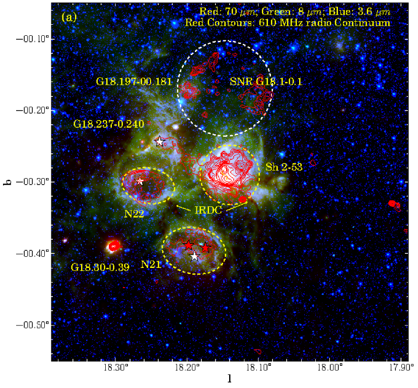
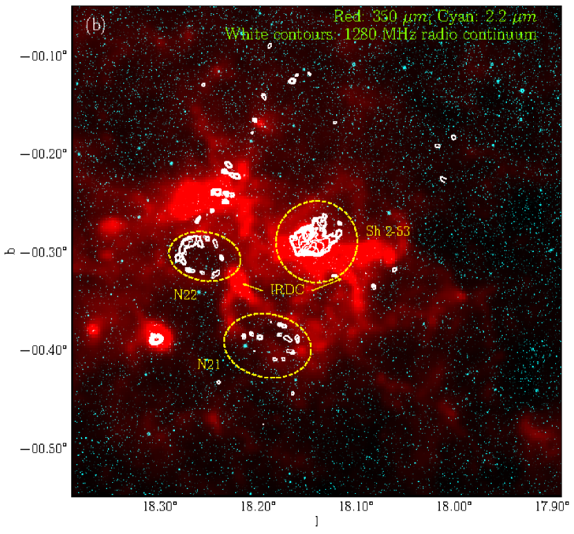
Figure 1.— (a) A color-composite image (red: 70 $\mu m$; green: 8.0 $\mu m$; blue: 3.6 $\mu m$) of 30${}^{\prime}\times$30^′ area around the Sh 2-53 region. The 610 MHz GMRT radio contours at levels of 3, 4, 5, 6, 8, 10, 12, 15, 20, 25, 30, and 40 mJy are also overlaid on the image. Several H ii regions, two MIR Galactic bubbles, IRDCs and a SNR are seen along the line of sight. The positions of the bubbles, Sh 2-53 region, and SNR are marked by ellipses and circles, respectively. The positions of spectroscopically confirmed O-stars (Paron et al., 2013) are also marked by white stars, while two more photometrically identified O-stars towards the N21 bubbles (Watson et al., 2008) are marked by red stars. (b) A two color-composite image of the region (red: 350 $\mu m$; cyan: 2.2 $\mu m$). The 1280 MHz GMRT contours at levels of 2.0, 2.5, 3.0, 5.0, 8.0, 12.0, 15.0, 20.0, 30.0, and 100.0 Jy are also overlaid on the image.

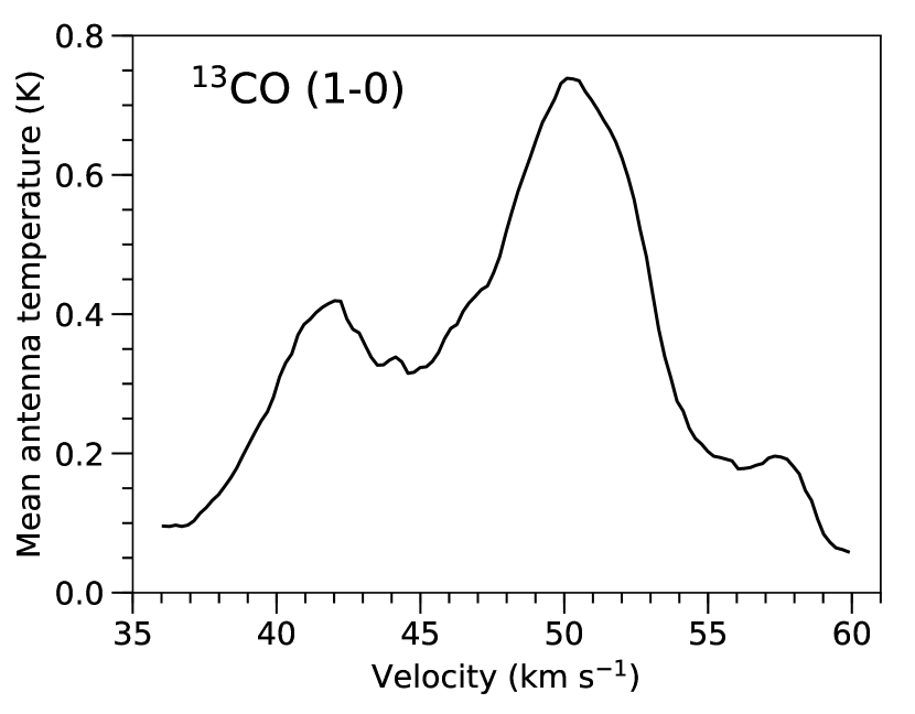
Figure 2.— The ¹³CO spectrum towards the S53 complex obtained by averaging the whole emission for the selected 30${}^{\prime}\times$30^′ area centered at $l=$ 18^∘.140, $b=$-0^∘.300. Three peaks are clearly depicted in the spectrum.

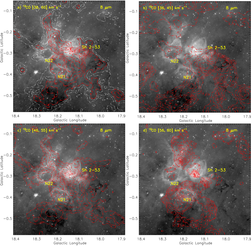
Figure 3.— (a) The velocity integrated ¹³CO contours for a velocity range from 36–60 km s^-1 are overlaid on the Spitzer 8 $\mu m$ image. In the direction of the S53 complex, three molecular clouds are traced within this velocity range. (b)–(d) The velocity integrated contours for velocity ranges from 36–45, 46–55, and 56–60 km s^-1, respectively, overlaid on the Spitzer 8 $\mu m$ image.

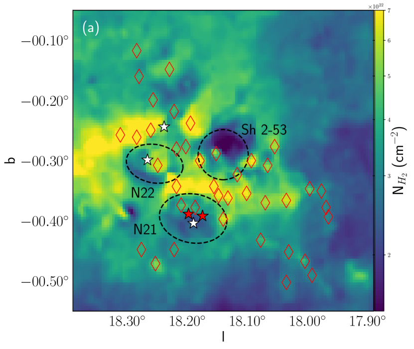
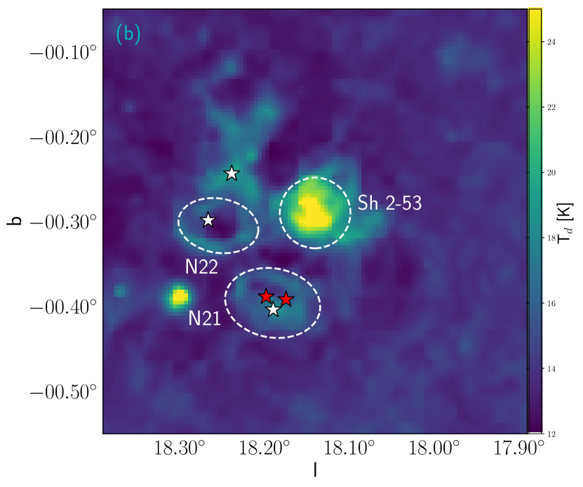
Figure 4.— Herschel (a) column density and (b) temperature maps of the S53 complex. Several cold clumps are also marked ($\diamond$) in the column density map. The remaining symbols are similar to those in Figure 1.

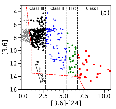
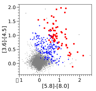
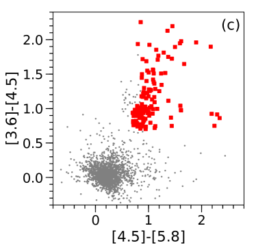
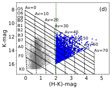
Figure 5.— The selection schemes of YSOs using the MIR and NIR color-color and color-magnitude criteria. (a) The [3.6]$-$[24]/[3.6] color-magnitude diagram of the point-like sources towards the region. Class I sources are marked by filled red squares. Flat-spectrum, Class II and Class III sources are marked by green filled pentagons, blue crosses, and black filled triangles, respectively. An extinction vector corresponding to $A_{K}$ of 5 mag is also shown. The sources in this scheme are selected and classified into different classes following the criteria outlined in Guieu et al. (2010) and Rebull et al. (2011). The red lines separates the YSOs from the field stars. (b) The color-color ([5.8]$-$[8.0]/[3.6]$-$[4.5]) diagram of point-like sources detected in all four Spitzer-IRAC bands. Elimination of possible contaminants and classification of remaining point sources are performed based on the scheme described in Gutermuth et al. (2009). (c) The color-color ([4.5]$-$[5.8]/[3.6]$-$[4.5]) diagram of those sources that are detected only in the first three Spitzer-IRAC bands among the four bands. The sources are classified following the criteria given in Hartmann et al. (2005) and Getman et al. (2007). (d) The NIR color-magnitude (H$-$K/K) diagram of all the reliable NIR sources detected in the $H$ and $K$ bands (see text for more details). A cutoff value of H$-$K of 2.0 mag was obtained from a nearby reference field ($12\arcmin\times 12\arcmin$ area centered at $l$ = 18^∘.12, $b$ = 0^∘.04).

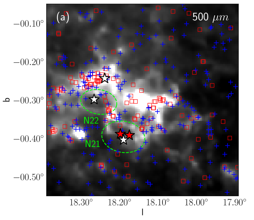
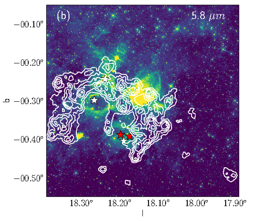
Figure 6.— (a) Class I and Class II YSOs, marked by red squares and blue crosses, respectively, overlaid on the 500 $\mu m$ image. The YSOs identified using the NIR scheme are not shown here, however, they are used in the surface density analysis. (b) Overlay of 20NN surface density contours (white) of all the YSOs on the Spitzer-IRAC 5.8 $\mu m$ image. The surface density contours of YSOs are drawn at 5, 7, 9, 12, 16, 20, 25 and 30 YSO pc^-2. YSOs are mainly clustered towards the junction of the Sh 2-53 region and the bubbles (see text for more details).

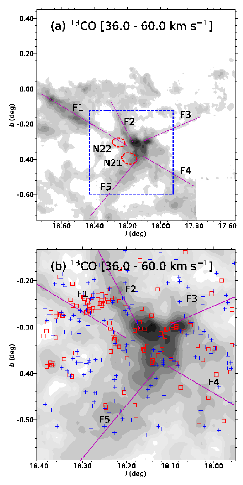
Figure 7.— (a) The velocity integrated ¹³CO map of a large 1^∘.2$\times$1^∘.2 area around the S53 complex for a velocity range of 36–60 km s^-1. Five filaments from F1–F5 are identified in this integrated molecular map, marked by magenta lines. Positions of the bubbles N21 and N22 are also marked and labeled. (b) The zoomed in view of ¹³CO map of the S53 complex, marked by a blue dashed box in panel (a). The positions of the Class I (red squares) and Class II (blue crosses) YSOs are also marked.

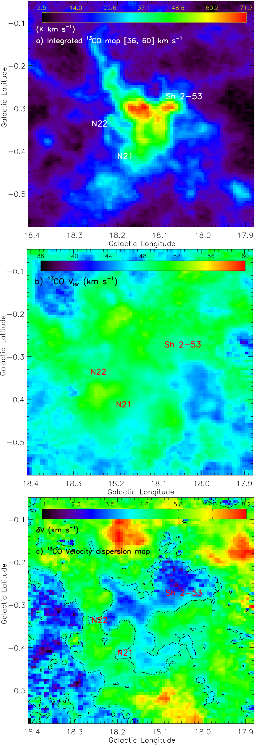
Figure 8.— (a) The velocity integrated ¹³CO map of the central region around the S53 complex for the velocity range of 36–60 km s^-1. (b) First moment or the velocity map of the region. (c) Second moment map or the velocity dispersion map of the S53 complex. Dispersion in the gas velocity can be clearly noted towards the S53 complex.

Figure 9.— (a)-(e) The $p-v$ diagrams for filaments F1–F5 marked in Figure 7. The peak velocities corresponding to the filaments and the central “hub” are marked by red and blue lines, respectively. Gradient in velocities in a range from 2-3 km s^-1 is noted almost for all the filaments within 5 pc towards the central “hub”. The broadening of the velocity profile can also be easily noted in the $p-v$ diagrams as these filaments move to the central “hub”.

Table 1The details of different sources and their association with the S53 complex.

Name of	l	b	$V_{LSR}$	Kinematic	Physical Association
the source	(deg)	(deg)	(km s-1)	Distance (kpc)	with the S53 complex
Bubble N21	18.190	–0.396	43.2	3.6	Yes
Bubble N22	18.254	–0.305	50.9	4.0	Yes
Sh 2–53	18.210	–0.320	52.0	4.3	Yes
G18.237–0.240	18.237	–0.240	47.0	–	Yes
SNR G18.1–0.1	18.106	–0.195	100.0	5.6	No
G18.197–0.181	18.197	–0.181	–	12.4	No
G18.30–0.39	18.303	–0.390	32.3	2.8	No

Table 2The dynamical ages of the H ii regions associated with the S53 complex seen in the 1280 MHz radio continuum map.

Name of the	Integrated 1280 MHz	Log of Lyman continuum	Spectral	Dynamical Age (Myr) for ambient density of
H ii region	Flux (Jy)	Flux (photons s-1)	type	1000 cm-3	2000 cm-3	5000 cm-3	10000 cm-3
N21	1.30	48.23	O8V	0.29	0.43	0.69	0.99
N22	1.60	48.32	O8V	0.28	0.41	0.66	0.94
Sh 2-53	4.74	48.79	O7V	0.18	0.27	0.45	0.65

References

- Anderson et al. (2009) Anderson, L. D., & Bania, T. M. 2009, ApJ, 690, 706
- André et al. (2016) André, P., Revéret, V., Könyves, V., et al. 2016, A&A, 592, A54
- Baug et al. (2015) Baug, T., Ojha, D. K., Dewangan, L. K., et al. 2015, MNRAS, 454, 4335
- Benjamin et al. (2003) Benjamin, R. A., Churchwell, E., Babler, B. L., et al. 2003, PASP, 115, 953
- Blitz et al. (1982) Blitz, L., Fich, M., & Stark, A. A. 1982, ApJS, 49, 183
- Carey et al. (2005) Carey, S. J., Noriega-Crespo, A., Price, S. D., et al. 2005, BAAS, 37, 63.33
- Churchwell et al. (2007) Churchwell, E., Watson, D. F., Povich, M. S., et al. 2007, ApJ, 670, 428
- Churchwell et al. (2006) Churchwell, E., Povich, M. S., Allen, D., et al. 2006, ApJ, 649, 759
- Cutri et al. (2003) Cutri, R. M., Skrutskie, M. F., van Dyk, S., et al. 2003, The 2MASS All Sky Catalog of Point Sources (available at https://www.ipac.caltech.edu/2mass/)
- Dale & Bonnell (2011) Dale, J. E., & Bonnell, I. 2011, MNRAS, 414, 321
- Dewangan et al. (2015) Dewangan, L. K., Luna, A., Ojha, D. K., et al. 2015, ApJ, 811, 79
- Dewangan et al. (2016) Dewangan, L. K., Ojha, D. K., Zinchenko, I., et al. 2016, ApJ, 833, 246
- Dewangan et al. (2016) Dewangan, L. K., Baug, T., Ojha, D. K., et al. 2016, ApJ, 826, 27
- Dewangan (2017) Dewangan, L. K. 2017, ApJ, 837, 44
- Dobashi et al. (1992) Dobashi, K., Yonekura, Y., Mizuno, A., & Fukui, Y. 1992, AJ, 104, 1525
- Elmegreen (1998) Elmegreen, B. G. 1998, in ASP Conf. Ser. 148, Origins, ed. C. E. Woodward, J. M. Shull, & H. A. Thronson, Jr. (San Francisco, CA: ASP), 150
- Evans et al. (2009) Evans, N. J., II, Dunham, M. M., Jrgensen, J. K., et al. 2009, ApJS, 181, 321
- Getman et al. (2007) Getman, K. V., Feigelson, E. D., Garmire, G., Broos, P., & Wang, J. 2007, ApJ, 654, 316
- Green (2014) Green, D. A. 2014, BASI, 42, 47
- Griffin et al. (2010) Griffin, M. J., Abergel, A., Abreu, A, et al. 2010, A&A, 518L, 3
- Guieu et al. (2010) Guieu, S., Rebull, L. M., Stauffer, J. R., et al. 2010, ApJ, 720, 46
- Gutermuth et al. (2009) Gutermuth, R. A., Megeath, S. T., Myers, P. C., et al. 2009, ApJS, 184, 18
- Gutermuth & Heyer (2015) Gutermuth, R. A., & Heyer, M. 2015, AJ, 149, 64
- Hacar et al. (2013) Hacar, A., Tafalla, M., Kauffmann, J., & Kovács, A. 2013, A&A, 554, A55
- Hartmann et al. (2005) Hartmann, L., Megeath, S. T., Allen, L., et al. 2005, ApJ, 629, 881
- Hildebrand (1983) Hildebrand, R. H. 1983, QJRAS, 24, 267
- Jackson et al. (2006) Jackson, J. M., Rathborne, J. M., Shah, R. Y., et al. 2006, ApJS, 163, 145
- Ji et al. (2012) Ji, W.-G., Zhou, J.-J., Esimbek, J., et al. 2012, A&A, 544, 39
- Jones et al. (2013) Jones, C., Dickey, J. M., Dawson, J. R., et al. 2013, ApJ, 774, 117
- Kassim et al. (1989) Kassim, N. E., Weiler, K. W., Erickson, W. C., & Wilson, T. L. 1989, ApJ, 338, 152
- Kilpatrick et al. (2016) Kilpatrick, C. D., Bieging, J. H., & Rieke, G. H. 2016, ApJ, 816, 1
- Kirk et al. (2013) Kirk, H., Myers, P. C., Bourke, T. L., et al. 2013, ApJ, 766, 115
- Kolpak et al. (2003) Kolpak, M. A., Jackson, J. M., Bania, T. M., Clemens, D. P., & Dickey, J. M. 2003, ApJ, 582, 756
- Kurtz (2002) Kurtz S., 2002, ASPC, 267, 81
- Kurtz (2002) Kurtz, S. 2002, in ASP Conf. Ser. 267, Hot Star Workshop III: The Earliest Phases of Massive Star Birth, ed. Crowther P. A. (San Francisco, CA: ASP), 81
- Lada et al. (2006) Lada, C. J., Muench, A. A., Luhman, K. L., et al. 2006, AJ, 131, 1574
- Launhardt et al. (2013) Launhardt, R., Stutz, A. M., Schmiedeke, A., et al. 2013, A&A, 551, A98
- Lawrence et al. (2007) Lawrence, A., Warren, S. J., Almaini, O., et al. 2007, MNRAS, 379, 1599
- Leahy et al. (2014) Leahy, D., Green, K., & Tian, W. 2014, MNRAS, 438, 1813
- Lockman (1989) Lockman, F. J. 1989, ApJS, 71, 469
- Lucas et al. (2008) Lucas, P. W., Hoare, M. G., Longmore, A., et al. 2008, MNRAS, 391, 136
- Mallick et al. (2013) Mallick, K. K., Kumar, M. S. N., Ojha, D. K., et al. 2013, ApJ, 779, 113
- Mallick et al. (2015) Mallick, K. K., Ojha, D. K., Tamura, M., et al. 2015, MNRAS, 447, 2307
- Moran (1983) Moran, J. M. 1983, RMxAA, 7, 95
- Motte et al. (2017) Motte, F., Bontemps, S., & Louvet, F. 2017, ARA&A, in press (arXiv:1706.00118)
- Myers (2009) Myers, P. C. 2009, ApJ, 700, 1609
- Nakamura & Li (2008) Nakamura, F., & Li, Z.-Y. 2008, ApJ, 687, 354-375
- Nakamura et al. (2014) Nakamura, F., Sugitani, K., Tanaka, T., et al. 2014, ApJ, 791, L23
- Olmi et al. (2016) Olmi, L., Cunningham, M., Elia, D., & Jones, P. 2016, A&A, 594, A58
- Omukai et al. (2005) Omukai, K., Tsuribe, T., Schneider, R., & Ferrara, A. 2005, ApJ, 626, 627
- Paron et al. (2013) Paron, S., Weidmann, W., Ortega, M. E., Albacete Colombo, J. F., & Pichel, A. 2013, MNRAS, 433, 1619
- Peretto et al. (2013) Peretto, N., Fuller, G. A., Duarte-Cabral, A., et al. 2013, A&A, 555, A112
- Poglitsch et al. (2010) Poglitsch, A., Waelkens, C., Geis, N., et al. 2010, A&A, 518, L2
- Pomarès et al. (2009) Pomarès, M., Zavagno, A., Deharveng, L., et al. 2009, A&A, 494, 987
- Rebull et al. (2011) Rebull, L. M., Johnson, C. H., Hoette, V., et al. 2011, AJ, 142, 25
- Samal et al. (2010) Samal, M. R., Pandey, A. K., Ojha, D. K., et al. 2010, ApJ, 714, 1015
- Schneider et al. (2012) Schneider, N., Csengeri, T., Hennemann, M., et al. 2012, A&A, 540, L11
- Schmeja et al. (2008) Schmeja, S., Kumar, M. S. N., & Ferreira, B. 2008, MNRAS, 389, 1209
- Sherman (2012) Sherman, R. A. 2012, ApJ, 760, 58
- Simpson et al. (2012) Simpson, R. J., Povich, M. S., Kendrew, S., et al. 2012, MNRAS, 424, 2442
- Skrutskie et al. (2006) Skrutskie, M. F., Cutri, R. M., Stiening, R., et al. 2006, AJ, 131, 1163
- Smith et al. (2002) Smith, L. J., Norris, R. P. F., & Crowther, P. A. 2002, MNRAS, 337, 1309
- Spitzer (1978) Spitzer, L. 1978, Physical processes in the interstellar medium, by Lyman Spitzer. New York Wiley-Interscience, 1978. 333 p.
- Stahler & Palla (2005) Stahler, S. W., & Palla, F. 2005, The Formation of Stars, by Steven W. Stahler, Francesco Palla, pp. 865. ISBN 3-527-40559-3. Wiley-VCH , January 2005., 865
- Strömgren (1939) Strömgren B., 1939, ApJ, 89, 526
- Tan et al. (2014) Tan, J. C., Beltrán, M. T., Caselli, P., et al. 2014, Protostars and Planets VI, 149
- Watson et al. (2008) Watson, C., Povich, M. S., Churchwell, E. B., et al. 2008, ApJ, 681, 1341
- Wienen et al. (2012) Wienen, M., Wyrowski, F., Schuller, F., et al. 2012, A&A, 544, 146
- Williams et al. (1994) Williams, J. P., de Geus, E. J., & Blitz, L. 1994, ApJ, 428, 693
- Zavagno et al. (2010a) Zavagno, A., Anderson, L. D., Russeil, D., et al. 2010, A&A, 518, L101
- Zavagno et al. (2010b) Zavagno, A., Russeil, D., Motte, F., et al. 2010, A&A, 518, L81
- Zhang et al. (2017) Zhang, C.-P., Yuan, J.-H., Xu, J.-L., et al. 2017, RAA, 17, 57