Three-dimensional vortex-bright solitons in a spin-orbit coupled spin-$1$ condensate

Abstract

We demonstrate stable and metastable vortex-bright solitons in a three-dimensional spin-orbit-coupled three-component hyperfine spin-1 Bose-Einstein condensate (BEC) using numerical solution and variational approximation of a mean-field model. The spin-orbit coupling provides attraction to form vortex-bright solitons in both attractive and repulsive spinor BECs. The ground state of these vortex-bright solitons is axially symmetric for weak polar interaction. For a sufficiently strong ferromagnetic interaction, we observe the emergence of a fully asymmetric vortex-bright soliton as the ground state. We also numerically investigate moving solitons. The present mean-field model is not Galilean invariant, and we use a Galilean-transformed mean-field model for generating the moving solitons.

I Introduction

A bright soliton, which arises due to a cancellation of the effects produced by non-linear and dispersive terms in the Hamiltonian, is a self-reinforcing solitary wave which maintains its shape while moving at a constant speed. Studies on the solitons have been done in a broad array of systems which include, among others, water waves, non-linear optics Kivshar , ultracold quantum gases including spinor Bose-Einstein condensates (BECs) Inouye ; li ; rb ; Perez-Garcia ; Ieda .

The spin-orbit (SO) coupling, the coupling between the spin and the center of mass motion of the atoms, is absent in the neutral atoms stringari . Nevertheless, a suitable modification of the atom-light interaction can generate a non-Abelian gauge potential Dalibard , thus subjecting the neutral atoms to the SO coupling. Guided by this idea, Lin et al. Lin experimentally generated an SO coupling with equal strengths of Rashba Rashba and Dresselhaus Dresselhaus terms in a BEC of ⁸⁷Rb in the two-component pseudo-spin-1/2 configuration, where one of the three spin components of the hyperfine spin-1 state of ⁸⁷Rb was removed from the experiment. This was achieved by dressing two of ⁸⁷Rb spin states from within its ground electronic manifold ($5S_{1/2},F=1$) with a pair of lasers Lin . More recently, SO coupling has been realized experimentally by Campbell et al. Campbell with the three hyperfine spin components of ⁸⁷Rb atoms. A lot of experimental studies have been done on SO-coupled BECs in recent years Aidelsburger .

It has been shown theoretically that the SO-coupled quasi-one-dimensional (quasi-1D) Salasnich ; rela , quasi-two-dimensional (quasi-2D) Xu ; Sakaguchi , and three-dimensional (3D) pu pseudo-spin-1/2 BECs can support solitonic structures. Bright solitons in SO-coupled three-component quasi-1D spin-1 Liu ; Gautam-3 and five-component spin-2 BECs Gautam-4 have also been theoretically investigated in addition to those in the three-component quasi-2D spin-1 BEC Gautam-5 .

In this paper, we demonstrate stable and metastable stationary and moving 3D vortex-bright solitons in a three-component SO-coupled hyperfine spin-1 BEC using a variational approximation and numerical solution of the mean-field Gross-Pitaevskii (GP) equation Ohmi . The effect of SO coupling on both an attractive and a weakly repulsive spinor BEC is to introduce attraction so as to form a soliton Sakaguchi . We find metastable vortex-bright solitons for $a_{0}+2a_{2}<0$, where $a_{0}$ and $a_{2}$ are the $s$-wave scattering lengths in the total spin 0 and 2 channels. The solitons can be stable for $a_{0}+2a_{2}\geq 0$. In the former case, the spinor BEC without SO-coupling is attractive, and the collapse cannot be stopped unconditionally thus producing only metastable solitons in the SO-coupled BEC for the number of atoms smaller than a critical number as in the case of a single-component quasi-one-dimensional attractive BEC li ; pg . In the latter case the spinor BEC can be purely repulsive and, because of this repulsion, it is possible to stop the collapse to form a stable soliton. In general, the implementation of SO-coupling in the three-component spin-1 BEC is more complicated than the same in the two-component pseudo-spin-1/2 BEC from both theoretical gtm and experimental Campbell points of view. Thus the present study goes beyond a previous investigation of 3D metastable bright solitons in pseudo-spin-1/2 BEC pu . Moreover, the parameter domain $(a_{0}+2a_{2}\geq 0)$ that leads to stable 3D vortex-bright solitons in a SO-coupled spin-1 BEC was not considered before in this context.

We observe that for small strengths of SO coupling, which we use in this investigation, the ground state vortex-bright soliton in the polar domain $(a_{2}>a_{0})$ has an antivortex and a vortex in $m_{f}=+1$ and $m_{f}=-1$ components, respectively, and a Gaussian-type structure in the $m_{f}=0$ component. The phase singularities in the $m_{f}=\pm 1$ components always coincide leading to axisymmetric density profiles for the component wavefunctions. We use phase-winding numbers Gautam-5 (angular momenta per particle in an axisymmetric system) of the three component wavefunctions to denote a vortex or an antivortex Mizushima . In terms of phase-winding numbers associated with the spin components $m_{f}=+1,0,-1$ Mizushima , this ground state vortex-bright soliton in the polar domain can be termed as symmetric and denoted $(-1,0,+1)$ corresponding to an anti-vortex in component $m_{f}=+1$ and a vortex in component $m_{f}=-1$. In the ferromagnetic domain ($a_{0}>a_{2}$), in addition to the axisymmetric vortex-bright solitons, asymmetric vortex-bright solitons with non-coinciding phase singularities in $m_{f}=\pm 1$ can also emerge as the ground state below a critical value of spin-exchange interaction parameter. In addition to this, we have also identified stationary excited axisymmetric vortex-bright solitons of type $(0,+1,+2)$ in both polar and ferromagnetic domains. Besides stationary vortex-bright solitons, we have also investigated the dynamically stable moving vortex-bright solitons of the SO-coupled spin-1 BEC using the Galelian-transformed coupled GP equations rela ; Sakaguchi ; Liu ; Gautam-3 .

The paper is organized as follows. In Sec. II.1, we describe the mean-field coupled Gross-Pitaevskii (GP) equations with Rashba SO coupling used to study the vortex-bright solitons in a spin-1 BEC. This is followed by a variational analysis of the stationary axisymmetric $(-1,0,+1)$ vortex-bright solitons in Sec. II.2. In Sec. III, we provide the details of the numerical method used to solve the coupled GP equations with SO coupling. We discuss the numerical results for axisymmetric vortex-bright solitons in Sec. IV.1, asymmetric solitons in Sec. IV.2, and moving solitons in Sec. IV.3. Finally, in Sec. V, we give a summary of our findings.

II Spin-Orbit coupled BEC vortex-bright soliton

II.1 Mean-field equations

For the study of a 3D vortex-bright soliton, we consider a trapless spin-1 spinor BEC. The single particle Hamiltonian of the BEC with Rashba Rashba SO coupling is H_zhai

$$H_{0}=\frac{p_{x}^{2}+p_{y}^{2}+p_{z}^{2}}{2m}+\gamma p_{x}\Sigma_{x}+\gamma p_{y}\Sigma_{y}+\gamma p_{z}\Sigma_{z},$$ (1)

where $p_{x}=-i\hbar\partial/\partial x$, $p_{y}=-i\hbar\partial/\partial y$, and $p_{z}=-i\hbar\partial/\partial z$ are the momentum operators along $x$, $y$, and $z$ axes, respectively, $m$ is the mass of each atom and $\Sigma_{x}$, $\Sigma_{y}$, and $\Sigma_{z}$ are the irreducible representations of the $x$, $y$, and $z$ components of the spin matrix, respectively,

$$\Sigma_{x} =\frac{1}{\sqrt{2}}\begin{pmatrix}0&1&0\\ 1&0&1\\ 0&1&0\end{pmatrix},\quad\Sigma_{y}=\frac{1}{\sqrt{2}i}\begin{pmatrix}0&1&0\\ -1&0&1\\ 0&-1&0\end{pmatrix},$$

$$\Sigma_{z}=\begin{pmatrix}1&0&0\\ 0&0&0\\ 0&0&-1\end{pmatrix},$$ (2)

and $\gamma$ is the strength of SO coupling. In the mean-field approximation, the SO-coupled 3D spin-1 BEC of $N$ atoms is described by the following set of three coupled GP equations, written here in dimensionless form, for different spin components $m_{f}=\pm 1,0$ Ohmi ; Kawaguchi

$$i\frac{\partial\psi_{\pm 1}(\mathbf{r})}{\partial t} ={\cal H}\psi_{\pm 1}(\mathbf{r})\pm c_{1}F_{z}\psi_{\pm 1}(\mathbf{r})+\frac{c_{1}}{\sqrt{2}}F_{\mp}\psi_{0}(\mathbf{r})$$

$$-\frac{i\gamma}{\sqrt{2}}\left(\frac{\partial\psi_{0}}{\partial x}\mp i\frac{\partial\psi_{0}}{\partial y}\pm\sqrt{2}\frac{\partial\psi_{\pm 1}}{\partial z}\right),$$ (3)

$$i\frac{\partial\psi_{0}(\mathbf{r})}{\partial t} ={\cal H}\psi_{0}(\mathbf{r})+\frac{c_{1}}{\sqrt{2}}[F_{-}\psi_{-1}(\mathbf{r})+F_{+}\psi_{+1}(\mathbf{r})]$$

$$-\frac{i\gamma}{\sqrt{2}}\Bigg{(}\frac{\partial\psi_{1}}{\partial x}+i\frac{\partial\psi_{1}}{\partial y}+\frac{\partial\psi_{-1}}{\partial x}-i\frac{\partial\psi_{-1}}{\partial y}\Bigg{)},$$ (4)

where ${\bf r}\equiv\{x,y,z\}$, ${\bf F}\equiv\{F_{x},F_{y},F_{z}\}$ is a vector whose three components are the expectation values of the three spin-operators over the multicomponent wavefunction, and is called the spin-expectation value Kawaguchi . Also,

$$F_{\pm}\equiv F_{x}\pm iF_{y}=\sqrt{2}[\psi_{\pm 1}^{*}(\mathbf{r})\psi_{0}(\mathbf{r})+\psi_{0}^{*}(\mathbf{r})\psi_{\mp 1}(\mathbf{r})],$$ (5)

$$F_{z}=n_{+1}(\mathbf{r})-n_{-1}(\mathbf{r}),\quad{\cal H}=-\frac{\nabla^{2}}{2}+c_{0}n(\bf r),$$ (6)

$$c_{0}=\frac{4N\pi(a_{0}+2a_{2})}{3l_{0}},~{}c_{1}=\frac{4N\pi({a_{2}-a_{0}})}{3l_{0}},$$ (7)

$$\nabla^{2}=\frac{\partial^{2}}{\partial x^{2}}+\frac{\partial^{2}}{\partial y^{2}}+\frac{\partial^{2}}{\partial z^{2}},$$ (8)

where $n_{j}({\bf r})=|\psi_{j}({\mathbf{r}})|^{2}$ with $j=\pm 1,0$ are the component densities, $n({\bf r})=\sum_{j}n_{j}({\bf r})$ is the total density, and asterisk denotes complex conjugate. The normalization condition satisfied by the component wavefunctions $\psi_{j}$ is

$$\int\sum_{j}n_{j}({\bf r})d{\bf r}=1.$$ (9)

All quantities in Eqs. (3)-(8) are dimensionless. This is achieved by writing length, density, time, and energy in units of $l_{0}$, $l_{0}^{-3}$, $ml_{0}^{2}/\hbar$, and $\hbar^{2}/(ml_{0}^{2})$, respectively, where $l_{0}$ is a scaling length and can be taken as $l_{0}=1$ $\mu$m. The energy of an atom in dimensionless unit is

$$E =\int d{\bf r}\biggr{[}\frac{1}{2}\biggr{\{}\sum_{j=-1}^{1}\left|\nabla\psi_{j}\right|^{2}+(c_{0}n^{2}+c_{1}|\mathbf{F}|^{2})\biggr{\}}-\frac{i\gamma}{\sqrt{2}}\psi_{0}^{*}\left(\frac{\partial\psi_{+1}}{\partial x}+\frac{\partial\psi_{-1}}{\partial x}\right)+\frac{\gamma}{\sqrt{2}}\psi_{0}^{*}\left(\frac{\partial\psi_{+1}}{\partial y}-\frac{\partial\psi_{-1}}{\partial x}\right)$$

$$-\frac{i\gamma}{\sqrt{2}}\left(\psi_{+1}^{*}+\psi_{-1}^{*}\right)\frac{\partial\psi_{0}}{\partial x}-\frac{\gamma}{\sqrt{2}}\left(\psi_{+1}^{*}-\psi_{-1}^{*}\right)\frac{\partial\psi_{0}}{\partial y}-i\gamma\left(\psi_{+1}^{*}\frac{\partial\psi_{1}}{\partial z}-\psi_{-1}^{*}\frac{\partial\psi_{-1}}{\partial z}\right)\biggr{]}.$$ (10)

It is instructive to analyze the SO-coupled system in the absence of interactions, i.e. $c_{0}=c_{1}=0$. Then, using Eqs. (1)-(2), the single particle SO-coupled Hamiltonian of the system is

$$H_{0} =\begin{pmatrix}-\frac{\nabla^{2}}{2}-i\gamma\frac{\partial}{\partial z}&-\frac{i\gamma}{\sqrt{2}}\partial_{-}&0\\ -\frac{i\gamma}{\sqrt{2}}\partial_{+}&-\frac{\nabla^{2}}{2}&-\frac{i\gamma}{\sqrt{2}}\partial_{-}\\ 0&-\frac{i\gamma}{\sqrt{2}}\partial_{+}&-\frac{\nabla^{2}}{2}+i\gamma\frac{\partial}{\partial z}\end{pmatrix},$$ (11)

where $\partial_{\pm}=\left(\frac{\partial}{\partial x}\pm i\frac{\partial}{\partial y}\right)$. The minimum eigen energy of the single particle Hamiltonian $H_{0}$ is $-\gamma^{2}/2$ and corresponds to $|{\bf k}|\equiv\sqrt{k_{x}^{2}+k_{y}^{2}+k_{z}^{2}}=\gamma$, and the (unnormalized) eigen function corresponding to this energy is

$$\Psi \sim\frac{1}{2}\begin{pmatrix}e^{-i\varphi}(|{\bf k}|-k_{z})^{2}/k_{\rho}^{2}\\ -\sqrt{2}(|{\bf k}|-k_{z})/k_{\rho}\\ e^{i\varphi}\end{pmatrix}e^{i(k_{x}x+k_{y}y+k_{z}z)},$$ (12)

where $\varphi=\tan^{-1}(k_{y}/k_{x})$ is the angle made by the projection of $\bf k$ on the $xy$ plane with the $x$ axis and $k_{\rho}=\sqrt{k_{x}^{2}+k_{y}^{2}}$. A general circularly symmetric solution can be obtained by considering the superposition of degenerate eigen functions with fixed $|k_{z}|$ and all possible values of $\varphi$, i.e.

$$\,\Psi_{\rm gen} \sim\sum_{k_{z}=|k_{z}|,-|k_{z}|}\int_{0}^{2\pi}\frac{1}{2}\begin{pmatrix}e^{-i\varphi}(|{\bf k}|-k_{z})^{2}/k_{\rho}^{2}\\ -\sqrt{2}(|{\bf k}|-k_{z})/k_{\rho}\\ e^{i\varphi}\end{pmatrix}e^{i(k_{\rho}x\cos\varphi+k_{\rho}y\sin\varphi+k_{z}z)}d\varphi,$$ (13)

$$\sim\sum_{k_{z}=|k_{z}|,-|k_{z}|}\begin{pmatrix}\pi e^{i(k_{z}z+\theta)}J_{1}(k_{\rho}\rho)(|{\bf k}|-k_{z})^{2}/k_{\rho}^{2}\\ \pi e^{ik_{z}z}J_{0}(k_{\rho}\rho)(|{\bf k}|-k_{z})/k_{\rho}\\ -\pi e^{i(k_{z}z-\theta)}J_{1}(k_{\rho}\rho)\end{pmatrix},$$ (14)

where $\theta=\tan^{-1}({y/x})$, $\rho=\sqrt{x^{2}+y^{2}}$, and $J_{0}(k_{\rho}\rho)$ and $J_{1}(k_{\rho}\rho)$ are the Bessel functions of first kind of order 0 and 1, respectively. In the asymptotic region, $\rho\rightarrow\infty$, $J_{0}(k_{\rho}\rho)\sim\sqrt{2/(\pi k_{\rho}\rho)}\cos(k_{\rho}\rho-\pi/4)$ and $J_{1}(k_{\rho}\rho)\sim\sqrt{2/(\pi k_{\rho}\rho)}\sin(k_{\rho}\rho-\pi/4)$ demonstrating the oscillatory nature of the wave function. The actual values of $k_{\rho}$ and $k_{z}$ will depend upon the full minimization of energy functional Eq. (10) satisfying $k_{\rho}^{2}+k_{z}^{2}=\gamma^{2}$.

II.2 Vortex-bright soliton

We demonstrate the existence of two types of metastable and stable low-energy stationary axisymmetric vortex-bright solitons, classified using phase-winding numbers as $(-1,0,+1)$ and $(0,+1,+2)$, and an asymmetric vortex-bright soliton. Out of the former two, the $(-1,0,+1)$ vortex-bright soliton has the lower energy. We find that, in the polar domain ($c_{1}>0$), the $(-1,0,+1)$ vortex-bright soliton has coinciding phase singularities in $m_{f}=\pm 1$ components, which results in axially-symmetric density profiles of the component wavefunctions and is the ground state. In the ferromagnetic domain ($c_{1}<0$), below a critical $c_{1}$, in addition to $(-1,0,+1)$ and $(0,+1,+2)$ vortex-bright solitons, we observe the emergence of ground state vortex-bright solitons in which an antivortex in the $m_{f}=+1$ component does not coincide with a vortex in the $m_{f}=-1$ component. This results in an asymmetric density profile for the component wavefunctions. The higher energy $(0,+1,+2)$ vortex-bright solitons obtained numerically are always axially symmetric due to coinciding phase singularities. Equations (3)-(4) are invariant under transformations: $y\rightarrow-y$, $z\rightarrow-z$, $\psi_{m_{f}}(x,y,z)\rightarrow\psi_{-m_{f}}(x,-y,-z)$. Under these transformations, a symmetric $(-1,0,+1)$ vortex-bright soliton transforms to itself, whereas a symmetric $(0,+1,+2)$ vortex-bright soliton transforms to $(-2,-1,0)$ vortex-bright soliton. This implies that associated with the $(0,+1,+2)$ vortex-bright soliton there is always a degenerate $(-2,-1,0)$ vortex-bright soliton.

Numerically, we find that the longitudinal magnetization ${\cal M}=\int[{n_{+1}({\bf r})-n_{-1}({\bf r})}]d\bf r$ is zero for the symmetric $(-1,0,+1)$ and asymmetric vortex-bright solitons, whereas it is, in general, non-zero for the $(0,+1,+2)$ solitons. The $(-1,0,+1)$ vortex-bright soliton with zero magnetization $\cal M$ can be analyzed using the following variational ansatz pu

$$\psi_{\pm 1} =\left(A_{1}\sigma_{z}\mp i\sqrt{2}Bz\right)\frac{\rho e^{-\frac{\rho^{2}}{2\sigma_{r}^{2}}-\frac{z^{2}}{2\sigma_{z}^{2}}\mp i\tan^{-1}\frac{y}{x}}}{\pi^{3/4}\sigma_{r}^{2}\sigma_{z}^{3/2}},$$ (15)

$$\psi_{0} =i\frac{A_{2}}{\pi^{3/4}\chi_{r}\sqrt{\chi_{z}}}e^{-\frac{\rho^{2}}{2\chi_{r}^{2}}-\frac{z^{2}}{2\chi_{z}^{2}}},$$ (16)

where $A_{1},A_{2},B,$ are the variational amplitudes and $\sigma_{r},\sigma_{z},\chi_{r}$, and $\chi_{z}$ are the variational widths of the Gaussian ansatz. Normalization condition (9) imposes the following constraint

$$2A_{1}^{2}+2B^{2}+A_{2}^{2}=1$$ (17)

on the variational parameters $A_{1},A_{2}$ and $B$. The variational energy of the soliton, obtained by substituting Eqs. (15) and (16) in Eq. (10), is

$$E =\frac{2\left(A_{1}^{2}+B^{2}\right)}{\sigma_{r}^{2}}+\frac{A_{1}^{2}+3B^{2}}{2\sigma_{z}^{2}}+\frac{A_{2}^{2}}{4}\left(\frac{2}{\chi_{r}^{2}}+\frac{1}{\chi_{z}^{2}}\right)+\frac{c_{0}}{\pi^{3/2}}\biggr{[}\frac{A_{2}^{4}}{4\sqrt{2}\chi_{z}\chi_{r}^{2}}+\frac{\left(4A_{1}^{4}+4A_{1}^{2}B^{2}+3B^{4}\right)}{8\sqrt{2}\sigma_{r}^{2}\sigma_{z}}$$

$$+\frac{{2A_{2}^{2}\chi_{r}^{2}\left\{B^{2}\chi_{z}^{2}+A_{1}^{2}\left(\sigma_{z}^{2}+\chi_{z}^{2}\right)\right\}}}{\left(\sigma_{z}^{2}+\chi_{z}^{2}\right)^{3/2}\left(\sigma_{r}^{2}+\chi_{r}^{2}\right)^{2}}\biggr{]}-\frac{16A_{1}A_{2}\gamma\sigma_{r}^{2}\chi_{r}\sqrt{\sigma_{z}\chi_{z}}}{\left(\sigma_{r}^{2}+\chi_{r}^{2}\right)^{2}\sqrt{\left(\sigma_{z}^{2}+\chi_{z}^{2}\right)}}-2\sqrt{2}\frac{A_{1}B\gamma}{\sigma_{z}},$$ (18)

This energy is independent of $c_{1}$ as ${\bf F}({\bf r})=0$ for symmetric $(-1,0,+1)$ vortex-bright soliton which is consistent with the choice of variational ansatz in Eqs. (15)-(16). Energy (18) can be minimized with respect to all variational parameters subject to the constraint (17) to obtain the minimum-energy ground state.

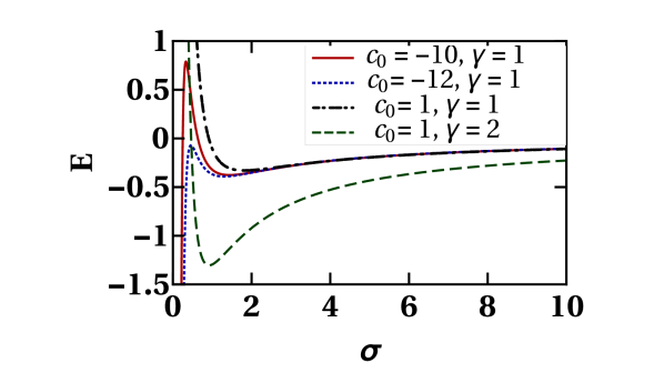
Figure 1: The variational energy (19) of a self-trapped 3D vortex-bright soliton as a function of width $\sigma$ for the parameters $c_{0}=1,-10,-12,c_{1}>0,\gamma=1,2$. A metastable vortex-bright soliton corresponds to a local minimum in energy as appears for $c_{0}<0$. A stable vortex-bright soliton can appear for $c_{0}\geq 0$.

To understand the role of SO coupling in the creation of self-trapped vortex-bright solitons, let us assume that the widths of the component wavefunction are of the same order of magnitude, say $\sigma_{r}=\sigma_{z}=\chi_{r}=\chi_{z}\approx\sigma$. In this case, energy (18) becomes

$$E =\left[\frac{\left(10A_{1}^{2}+3A_{2}^{2}+14B^{2}\right)}{4\sigma^{2}}\right]-\left(\frac{2\sqrt{2}A_{1}\left(A_{2}+B\right)\gamma}{\sigma}\right)$$

$$+\left\{{c_{0}}\frac{4A_{1}^{4}+2A_{2}^{4}+2A_{2}^{2}B^{2}+3B^{4}+4A_{1}^{2}\left(A_{2}^{2}+B^{2}\right)}{8\sqrt{2}\pi^{3/2}\sigma^{3}}\right\},$$

$$\equiv\left[\frac{C_{1}}{\sigma^{2}}\right]-\left(\frac{\gamma C_{2}}{\sigma}\right)+\left\{\frac{c_{0}C_{3}}{\sigma^{3}}\right\},$$ (19)

where $C_{1},C_{2},C_{3}$ are the functions of $A_{1}$ and $B$ (as $A_{2}$ itself is a function of $A_{1}$ and $B$) and are all greater than zero. If we let, $A_{1}$ and $B$ to assume all possible real values greater than zero, then the total energy has a local minimum at

$$\sigma=\frac{C_{1}+\sqrt{C_{1}^{2}+3\gamma c_{0}C_{2}C_{3}}}{\gamma C_{3}},$$ (20)

provided $\gamma>0$ and $C_{1}^{2}+3\gamma c_{0}C_{2}C_{3}>0$, the latter inequality implies that the dispersive effects are strong enough to prevent the collapse of the system.

To see explicitly, how a metastable (stable) self-trapped symmetric $(-1,0,+1)$ vortex-bright soliton corresponds to local (global) minimum of energy, we minimize energy (18) and calculate all seven variational parameters: $\sigma_{r},\sigma_{z},\chi_{r},\chi_{z},A_{1},A_{2}$ and $B$. Using the values of $A_{1},B$, and $A_{2}$ so obtained, we calculate the variation of energy (19) as a function of the width $\sigma$. The resulting $E$ versus $\sigma$ curves are shown in Fig. 1 for different $c_{0}$ and a fixed SO coupling $\gamma$ illustrating a local minimum and also the collapse as $\sigma\rightarrow 0$ for $c_{0}<0$: energy $E\to-\infty$ as $\sigma\rightarrow 0$. For $c_{0}\geq 0$, there could be a global minimum with no possibility of collapse and one has a stable soliton. We see in Fig. 1 that the minimum of the energy is more pronounced for a larger spin-orbit coupling $\gamma$, thus leading to stronger binding. The case $c_{0}\geq 0,c_{1}=\gamma=0$ corresponds to a repulsive spinor condensate. For $0>c_{0}>c_{\mathrm{crit}}$, only a local minimum of energy is possible and the vortex-bright soliton is metastable, whereas, for $c_{0}<c_{\mathrm{crit}}$, no localized soliton is possible and the system collapses. In contrast, a quasi-two-dimensional (quasi-2D) self-trapped vortex-bright soliton is always stable and corresponds to a global minimum of energy Gautam-5 .

One can also look at the variation of energy (18) by fixing $A_{1},B$, and hence $A_{2}$ and two variational parameters characterizing the widths of the components as a function of the remaining two variational widths. For this purpose, we find the variational parameters $A_{1},B,A_{2},\sigma_{r},\chi_{r},\chi_{z}$ and $\sigma_{z}$ corresponding to the minimum of energy (18), which is a function of these parameters. Fixing the parameters $A_{1},B,A_{2},\chi_{r},$ and $\chi_{z}$ at the values corresponding the minimum of energy (18), we consider energy as a function of the widths $\sigma_{r}$ and $\sigma_{z}$ and present its contour plot in Fig. 2(a) illustrating the variation of $E$ as a function of widths of $m_{f}=\pm 1$ components. Similarly in Fig. 2(b), we show the variation of $E$ as a function of widths of the $m_{f}=0$ component fixing the variational parameters $A_{1},B,A_{2},\sigma_{r},$ and $\sigma_{z}$ at the minimum of energy. For large widths ($\sigma_{r},\sigma_{z},\chi_{r},\chi_{z}\to\infty$) in Fig. 2 the energy vanishes ($E\to 0$). The geometric mean of the widths corresponding to the local minima in Figs. 2(a) and (b) is $1.3$ and is close to the approximate width $\sigma$ corresponding to the minimum in Fig. 1 as should be the case.

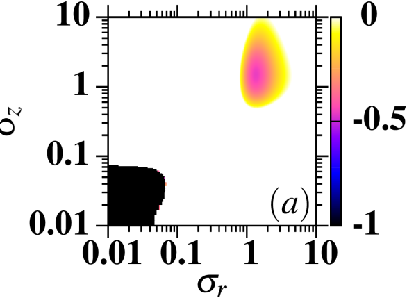
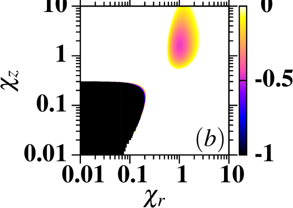
Figure 2: (a) Contour plot variational energy as a function of radial and axial widths of $m_{f}=\pm 1$ components, (b) the same as a function of radial and axial widths of $m_{f}=0$ component. The local minimum of energy corresponding to the vortex-bright solitons as well as the collapse near the origin are highlighted. The interaction parameters are $c_{0}=-10,c_{1}>0,\gamma=1$. See the text for further details.

III Numerical Procedure

The coupled equations (3)-(4) can be solved by time-splitting Fourier pseudo-spectral method psanand ; Wang and time-splitting Crank-Nicolson method Bao ; Muruganandam . Here, we extend the Fourier pseudo-spectral method to the coupled GP equations with SO-coupling terms and use the same to solve Eqs. (3)-(4). The coupled set of GP equations (3)-(4) can be represented in a simplified form as

$$\frac{i\partial\Psi}{\partial t}=\left({H_{1}+H_{2}+H_{3}}\right)\Psi,$$ (21)

where $\Psi=(\psi_{+1},\psi_{0},\psi_{-1})^{T}$ with $T$ denoting the transpose, $H_{1}$, $H_{2}$ and $H_{3}$ are $3\times 3$ matrix operators defined as

$$H_{1} =\begin{pmatrix}{\cal H}^{-}+c_{1}(n_{0}+n_{-})&0&0\\ 0&{\cal H}+c_{1}n_{+}&0\\ 0&0&{\cal H}^{+}+c_{1}(n_{0}-n_{-})\end{pmatrix},$$ (22)

$$H_{2} =\begin{pmatrix}0&c_{1}\psi_{0}\psi_{-1}^{*}&0\\ c_{1}\psi_{0}^{*}\psi_{-1}&0&\psi_{0}^{*}\psi_{+1}\\ 0&c_{1}\psi_{0}\psi_{+1}^{*}&0\end{pmatrix},$$ (23)

$$H_{3} =-i\frac{\gamma}{\sqrt{2}}\begin{pmatrix}0&\partial_{-}&0\\ \partial_{+}&0&\partial_{-}\\ 0&\partial_{+}&0\end{pmatrix},$$ (24)

where

$${\cal H}^{\mp}={\cal H}\mp i\gamma\frac{\partial}{\partial_{z}},\quad n_{\pm}=n_{+1}\pm n_{-1},\quad$$ (25)

Now, in the time-splitting method the following equations are solved successively

$$\frac{i\partial\Psi}{\partial t} = H_{1}\Psi,$$ (26)

$$\frac{i\partial\Psi}{\partial t} = H_{2}\Psi,$$ (27)

$$\frac{i\partial\Psi}{\partial t} = H_{3}\Psi.$$ (28)

Equation (26) can be numerically solved using Fourier pseudo-spectral method Wang which we employ in this paper or semi-implicit Crank-Nicolson method Muruganandam and involves additional time-splitting of $H_{1}$ into its spatial derivative and non-derivative parts. The numerical solutions of Eq. (27) have been discussed in Refs. Wang ; Martikainen . We use Fourier pseudo-spectral method to accurately solve Eq. (28). In Fourier space, Eq. (28) is

$$\frac{i\partial\widetilde{\Psi}}{\partial t}=\widetilde{H}_{3}\widetilde{\Psi},$$ (29)

where tilde indicates that the quantity has been Fourier transformed. Hamiltonian $H_{3}$ in Fourier space is

$$\widetilde{H}_{3}=-i\frac{\gamma}{\sqrt{2}}\begin{pmatrix}0&ik_{x}+k_{y}&0\\ ik_{x}-k_{y}&0&ik_{x}+k_{y}\\ 0&ik_{x}-k_{y}&0\end{pmatrix}$$ (30)

The solution of Eq. (29) is

$$\widetilde{\Psi}(t+dt) =e^{-i\widetilde{H}_{3}dt}\widetilde{\Psi}(t)=e^{-i\hat{O}}\widetilde{\Psi}(t),$$ (31)

$$=\left(I+\frac{\cos{\Omega}-1}{\Omega^{2}}\hat{O}^{2}-i\frac{\sin{\Omega}}{\Omega}\hat{O}\right)\widetilde{\Psi}(t),$$ (32)

where $\Omega=\sqrt{|A|^{2}+|B|^{2}}$, where $A=-i\frac{\gamma}{\sqrt{2}}\left(ik_{x}+k_{y}\right)dt$ and $B=-i\frac{\gamma}{\sqrt{2}}\left(ik_{x}-k_{y}\right)dt$, and $\hat{O}$ is defined as

$$\hat{O}=\begin{pmatrix}0&A&0\\ A^{*}&0&B^{*}\\ 0&B&0\end{pmatrix}.$$ (33)

The wavefunction in Eq. (32) is in Fourier space and can be inverse Fourier transformed to obtain the solution in configuration space. In this study, in space and time discretizations, we use space and time steps of $0.1$ and $0.005$, respectively, in imaginary-time simulation, whereas in real-time simulation these are, respectively, $0.1$ and $0.0005$. Numerically, the component wave functions of a stationary $(-1,0,+1)$ vortex-bright soliton are calculated by an imaginary-time propagation of Eqs. (3) and (4) using the initial guess of component wave functions (15) and (16).

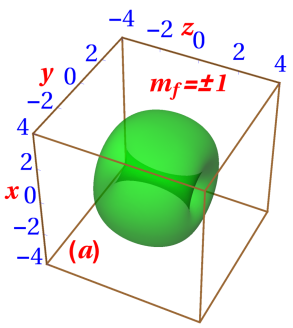
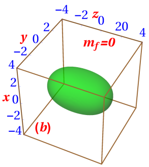
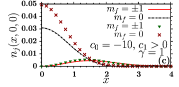
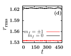
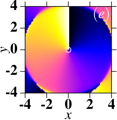
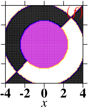
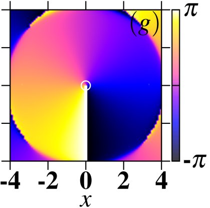
Figure 3: (a) Numerical isodensity contour of $|\psi_{m_{f}}|^{2}$ for $m_{f}=\pm 1$ components for $c_{0}=-10,c_{1}\geq 0$, and $\gamma=1$ in an axisymmetric $(-1,0,+1)$ vortex-bright soliton, (b) the same for the $m_{f}=0$ component. The density on the contour is 0.0007.(c) Numerical (line) and variational (chain of symbols) results for radial densities in the $z=0$ plane $n_{j}(x,0,0)$ versus $x$. (d) Numerical result of rms sizes of the component wave functions versus time as obtained in real-time simulation of the solution shown in (a)-(c); upper-black(dark) and lower-red(light) curves correspond to rms sizes of $m_{f}=0$ and $m_{f}=\pm 1$ components, respectively. All quantities in this and following figures are dimensionless. (e), (f) and (g) show the phase distribution of $m_{f}=+1$, $m_{f}=0$, and $m_{f}=-1$ components, respectively, in $z=0$ plane. The norms $\int n_{j}d{\bf r}$ of three components obtained numerically are 0.29, 0.42, and 0.29, for $j=1,0,$ and $-1$, respectively.

IV Numerical results

IV.1 Axisymmetric vortex-bright soliton

First we consider the $(-1,0,+1)$ vortex-bright soliton in the polar domain. The numerical results for surfaces of constant density (isodensity contour) in coordinate space for an axisymmetric $(-1,0,+1)$ vortex-bright soliton with $c_{0}=-10,c_{1}\geq 0$, and $\gamma=1$ are shown in Figs. 3(a)-(b). In the polar domain, $c_{1}>0$, the results for $(-1,0,+1)$ vortex-bright solitons are independent of the parameter $c_{1}$. To compare the numerical and variational results, we show in Fig. 3(c) the numerical and variational densities in the radially outward direction $n_{j}(x,0,0)$ versus $x$ in the $z=0$ plane. In the $z=0$ plane, the densities of the three components have the oscillating asymptotic behavior given by $n_{\pm 1}(x,y,0)\sim J_{1}(k_{\rho}\rho)^{2}$ and $n_{0}(x,y,0)\sim J_{0}(k_{\rho}\rho)^{2}$ as discussed in Sec. II.1. The Gaussian ansatz does not capture the oscillating tail properly resulting in the difference in numerical and variational results in Fig. 3(c). To demonstrate the dynamical stability of the vortex-bright soliton, we performed real-time simulation of the imaginary-time profile as the initial state over a long interval of time. The dynamical stability in real time propagation confirm a stable ground state or a metastable state. The steady oscillation of the root-mean-square (rms) size ($r_{\mathrm{rms}}\equiv\sqrt{x_{\mathrm{rms}}^{2}+y_{\mathrm{rms}}^{2}+z_{\mathrm{rms}}^{2}}$   ) of the components as shown in Fig. 3 (d), corresponding to the $(-1,0,+1)$ vortex-bright soliton shown in Figs. 3 (a)-(c), demonstrates the dynamical stability of the soliton. The nature of phase singularity, if any, in the components can be inferred from the phase plots of three components in $z=0$ plane as are shown in Figs. 3(e)-(g), where the location of the vortex is indicated by a small circle in the phase plots.

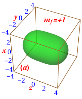
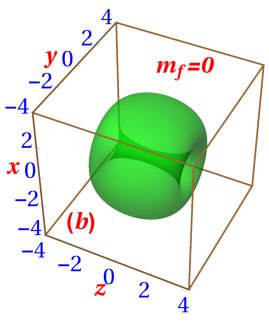
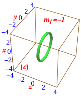
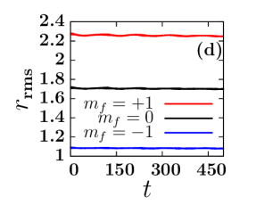
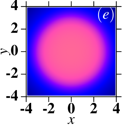
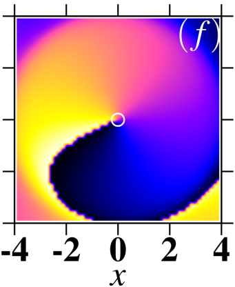
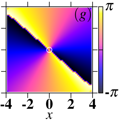
Figure 4: Numerical isodensity contour of $|\psi_{m_{f}}|^{2}$ for (a) $m_{f}=+1$, (b) $m_{f}=0$, and (c) $m_{f}=-1$ components of a polar $(0,+1,+2)$ vortex-bright soliton for $c_{0}=-10,c_{1}=0.1$ and $\gamma=1$. The density on the contour is 0.0007. The isosurfaces are translucent to show the presence of vortex lines. (d) Numerical result of rms size ($r_{\mathrm{rms}}$) of the component wave functions versus time as obtained in real-time simulation of the solution shown in (a)-(c); upper-red, middle-black and lower-blue curves correspond to $m_{f}=+1$, $m_{f}=0$, and $m_{f}=-1$ components, respectively. (e), (f) and (g) show the phase distribution of $m_{f}=+1$, $m_{f}=0$, and $m_{f}=-1$ components, respectively, in $z=0$ plane. The norms of the three components are 0.63, 0.29, 0.09 for $m_{f}=+1$, $m_{f}=0$, and $m_{f}=-1$ respectively.

The numerical isodensity contour of the axisymmetric $(0,+1,+2)$ vortex-bright soliton for $c_{0}=-10$, $\gamma=1$ and $c_{1}=0.1$ are shown in Figs. 4(a)-(c). The results for the axisymmetric $(0,+1,+2)$ vortex-bright soliton in the polar domain depend on the value of $c_{1}$. The numerical result is obtained by an imaginary-time simulation of Eqs. (3) and (4) with the initial guess of component wave functions $\psi_{1}^{\mathrm{inital}}\approx\psi_{\rm Gauss},~{}\psi_{0}^{\mathrm{inital}}\approx(x+iy)\psi_{\rm Gauss},~{}\psi_{-1}^{\mathrm{inital}}\approx(x+iy)^{2}\psi_{\rm Gauss}$, where $\psi_{\rm Gauss}$ is a Gaussian wavefunction. The $(0,+1,+2)$ vortex-bright soliton shown in 4(a)-(c) has higher energy than the $(-1,0,+1)$ soliton shown in Figs. 3(a)-(c). Again, the $(0,+1,+2)$ vortex-bright soliton is dynamically stable as is demonstrated by the steady oscillation of rms sizes of the component wavefunctions in Fig. 4(d). We do not observe any decay of the angular momentum in each component in both $(-1,0,+1)$ and $(0,+1,+2)$ vortex-bright solitons. The charge of the vortices in the three components is evident from the phase-profile of three components shown in Figs. 4(g)-(f) with a small circle used to indicate the exact location of phase singularity.

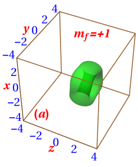
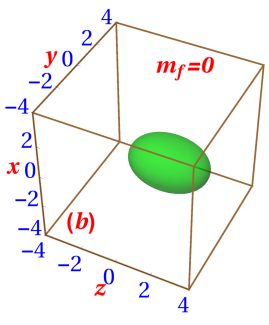
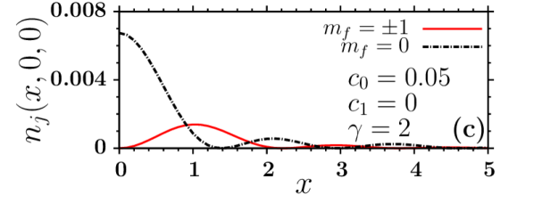
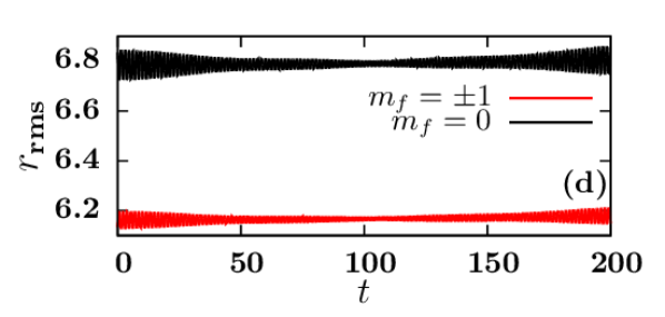
Figure 5: Numerical isodensity contour of $|\psi_{m_{f}}|^{2}$ for (a) $m_{f}=\pm 1$, (b) $m_{f}=0$, components of an axisymmetric (-1,0,+1) soliton with $c_{0}=0.05$, $c_{1}=0$ and $\gamma=2$. The density on the contour is 0.001. (c) Numerical results for radial densities in the $z=0$ plane $n_{j}(x,0,0)$ versus $x$. (d) Numerical result of rms sizes of the component wave wavefunctions versus time as obtained in real-time simulation of the solution shown in (a)-(c); upper-black(dark) and lower-red(light) curves correspond to $m_{f}=0$ and $m_{f}=\pm 1$ components, respectively. The norms of the three components are 0.30, 0.39, 0.30, for $m_{f}=+1,0$, and $m_{f}=-1$ components, respectively.

Solitons are also possible in a repulsive spinor BEC. Using variational approximation in Sec. II.2, we found that the SO-coupled BEC may have stable vortex bright soliton for $c_{0}\geq 0$, viz. Fig. 1. The numerical isodensity contour of such a (-1,0,+1) vortex-bright soliton with $c_{0}=0.05,c_{1}\geq 0$, and $\gamma=2$ are shown in Figs. 5(a)-(b). Although a larger $\gamma$ leads to easier bright-soliton formation, viz. Fig. 1, we could not use a much larger $\gamma$ because of the numerical difficulty in treating a large undulating tail in density str , associated with a large $\gamma$. In asymptotic region in the $xy$ plane, the densities of the $m_{f}=\pm 1$ and $m_{f}=0$ components vary as $\sim\sin(k_{\rho}\rho-\pi/4)$ and $\sim\cos(k_{\rho}\rho-\pi/4)$, respectively, viz. Sec. II.1 leading to the oscillating tail with period inversely dependent on $k_{\rho}=\sqrt{\gamma^{2}-k_{z}^{2}}$. The long-time oscillation in the rms radius $r_{\rm rms}$ of the three components, corresponding to the $(-1,0,+1)$ vortex-bright soliton shown in Figs. 5(a)-(c), as obtained upon real-time evolution of the imaginary-time profile exhibited in Fig. 5(d), establishes the dynamical stability of the soliton.

A finite space step $\Delta x$ and a finite space domain $L$ of discretization along the corresponding direction set a limit on the accuracy of the numerical scheme. The typical wavelength of spatial modulations of density should be much larger than the space step for an adequate resolution and for obtaining reliable results $-$ a condition which is very well satisfied for the SOC values considered in the present work. Larger SOC values will require even smaller space step to adequately treat the high-wavenumber spatial modulations of density. For example, comparing the density plots of Figs. 3(c) and 5(c), we find that a larger SOC ($\gamma=2$) in the latter has led to pronounced spatial modulations of density compared to the former with a smaller SOC ($\gamma=1$). The use of the same spatial step ($\Delta x=0.1$) in both cases has set a limit on the accuracy in Fig. 5(c), which is responsible for the rapid temporal oscillation of the rms size in Fig. 5(d). Also, the space domain $L$ should be much larger than the size of the condensate along that direction for obtaining accurate results. However, any finite $L$ leads to the slow temporal oscillation of the rms size in Fig. 3(d), which is also present in Fig. 5(d) as a modulating envelope over the rapid oscillation. As the space domain $L$ is increased these oscillations with smaller frequency will tend to vanish. The use of small space step will reduce the fast temporal oscillations of the rms size in Fig. 5(d), whereas larger space domain will suppress the slow oscillation of the rms size.

IV.2 Asymmetric solitons

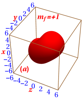
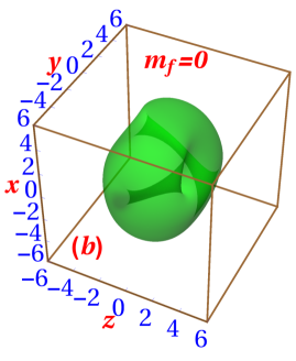
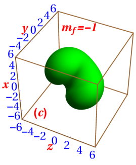
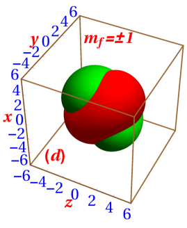
Figure 6: Numerical isodensity contour of $|\psi_{m_{f}}|^{2}$ for (a) $m_{f}=+1$, (b) $m_{f}=0$, (c) $m_{f}=-1$ components of an asymmetric soliton with $c_{0}=-10$, $c_{1}=-1$ and $\gamma=1$. The density on the contour is 0.00008. (d) shows the isosurfaces in (a) and (c) together. The norms of three components are $0.32$, $0.36$, $0.32$ for $m_{f}=+1,0$, and $m_{f}=-1$, respectively.

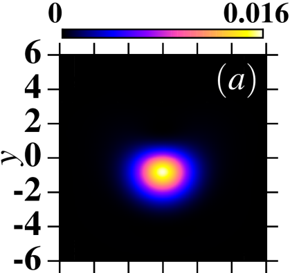
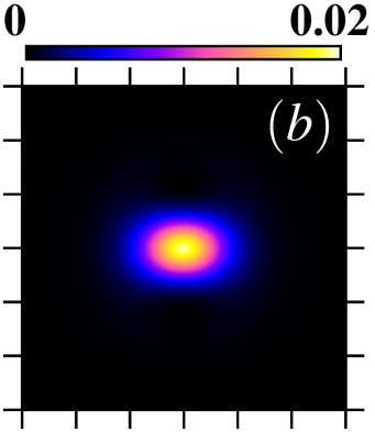
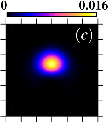
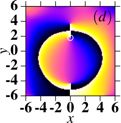
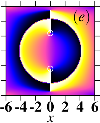
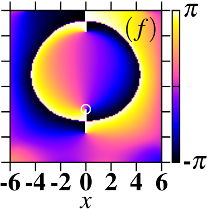
Figure 7: The 2D contour plots of densities of components in $z=0$ plane, corresponding to isodensity contours shown in 6, for (a) $m_{f}=+1$, (b) $m_{f}=0$, (c) $m_{f}=-1$ components of an asymmetric soliton with $c_{0}=-10$, $c_{1}=-1$ and $\gamma=1$. The corresponding phases are shown in (d) for $m_{f}=+1$, (e) for $m_{f}=0$, and (f) for $m_{f}=-1$ components.

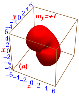
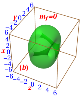
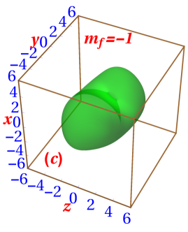
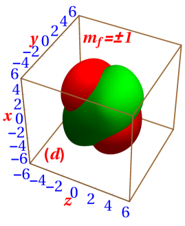
Figure 8: Numerical isodensity contour of $|\psi_{m_{f}}|^{2}$ for the components (a) $m_{f}=+1$, (b) $m_{f}=0$, (c) $m_{f}=-1$ of a moving vortex-bright soliton with $c_{0}=-10,$ $c_{1}=0.1$, $\gamma=1$, and $v=0.01$ towards positive $x$ direction. The density on the contour is $0.00008$. (d) shows the isosurfaces in (a) and (c) together. The norms of three components are $0.31$, $0.38$, $0.31$ for $m_{f}=+1,0$, and $m_{f}=-1$, respectively.

In the ferromagnetic domain ($c_{1}<0$) below a critical $c_{1}$, the system, in addition to axisymmetric vortex-bright solitons considered above, can also support an asymmetric vortex-bright soliton, which is found to be of lower energy than the axisymmetric ones and hence becomes the ground state. The 3D numerical isodensity contours of the component wave functions for the asymmetric vortex-bright soliton with $c_{0}=-10$, $c_{1}=-1$ and $\gamma=1$ are shown in Figs. 6(a)-(c). The corresponding 2D contour densities and phase profiles in $z=0$ plane are shown in Fig. 7(a)-(f). The density on the contour (=0.00008) in Fig. 6 is much smaller than those in Figs. 3, 4, and 5 and hence the sizes of solitons in Fig. 6 look larger and these plots reveal interesting vortex structure in the outer region of low density, which would not have been visible if a larger density on the contour were chosen. For $c_{0}=-10$ and $\gamma=1$, the asymmetric solitons exist for $-0.1\leq c_{1}\leq-2.7$. Below $c_{1}=-2.7$, no self-trapped solutions exist for $c_{0}=-10$ and $\gamma=1$, and the system collapses due to an excess of attractive interactions. In an asymmetric vortex-bright soliton, we find an antivortex line in component $m_{f}=+1$ (phase winding number $-1$) and a vortex line in component $m_{f}=-1$ (phase winding number $+1$) which are perpendicular to each other and displaced from the $z$ axis and also from each other. The asymmetrically located antivortex and vortex lines in the $m_{f}=\pm 1$ components lead to the kidney-shaped density distributions for these two components which fit into each other as shown in Fig. 6(d). There are mutually perpendicular and laterally displaced antivortex and vortex lines of winding numbers $\mp 1$ in the $m_{f}=0$ component too located in regions $y>0$ and $y<0$, respectively, viz. Fig. 6(b). These line vortices do not coincide with the line vortices present in the $m_{f}=\pm 1$ components. In Fig. 7(d)-(f), the phase-singularities corresponding to holes (depressions) in 3D isodensity contours of $m_{f}=0$ $(m_{f}=\pm 1)$ component are shown enclosed by small white circles. By writing the GP equations (3)-(4) in spherical polar coordinates ($r,\theta,\phi$), it can be seen that these are invariant under the transformations: $\phi\rightarrow\phi+\delta\phi$ and $\psi_{m_{f}}(r,\theta,\phi)\rightarrow\psi_{m_{f}}(r,\theta,\phi+\delta\phi)e^{-im_{f}\delta\phi}$; here $r,\theta,\phi$ are radial, polar and azimuthal coordinates. It implies that by rotating the density isosurfaces shown in Fig. 6 about $z$ axis, we can get innumerable possible degenerate asymmetric vortex-bright solitons. In experiments, this rotation symmetry about $z$ axis will be spontaneously broken with the emergence of one of these asymmetric solitons.

IV.3 Dynamically stable moving solitons

The GP equations (3)-(4) are not Galilean invariant as can be shown by using Galilean transformation $x^{\prime}=x-vt,y^{\prime}=y,z^{\prime}=z,t^{\prime}=t$, where $v$ is the relative velocity along $x$ axis of the primed coordinate system with respect to unprimed coordinate system, along with the transformation

$$\psi_{j}(x,y,z,t)=\psi^{\prime}_{j}(x^{\prime},y^{\prime},z^{\prime},t^{\prime})e^{ivx^{\prime}+iv^{2}t^{\prime}/2},$$ (34)

in Eqs. (3)-(4). This leads to the following Galilean-transformed mean-field GP equations Gautam-3

$$i\frac{\partial\psi_{\pm 1}^{\prime}(\mathbf{r}^{\prime})}{\partial t^{\prime}} ={\cal H}\psi_{\pm 1}^{\prime}(\mathbf{r}^{\prime})\pm c_{1}F_{z}^{\prime}\psi_{\pm 1}^{\prime}(\mathbf{r}^{\prime})+\frac{c_{1}}{\sqrt{2}}F_{\mp}^{\prime}\psi_{0}^{\prime}(\mathbf{r}^{\prime})$$

$$-\frac{i\gamma}{\sqrt{2}}\left(\frac{\partial\psi_{0}^{\prime}}{\partial x^{\prime}}\mp i\frac{\partial\psi_{0}^{\prime}}{\partial y^{\prime}}\pm\sqrt{2}\frac{\partial\psi_{\pm 1}^{\prime}}{\partial z^{\prime}}\right)+\frac{\gamma}{\sqrt{2}}v\psi_{0}^{\prime},$$ (35)

$$i\frac{\partial\psi_{0}^{\prime}(\mathbf{r}^{\prime})}{\partial t^{\prime}} ={\cal H}\psi_{0}^{\prime}(\mathbf{r}^{\prime})+\frac{c_{1}}{\sqrt{2}}[F_{-}^{\prime}\psi_{-1}^{\prime}(\mathbf{r}^{\prime})+F_{+}^{\prime}\psi_{+1}^{\prime}(\mathbf{r}^{\prime})]$$

$$-\frac{i\gamma}{\sqrt{2}}\Bigg{(}\frac{\partial\psi_{1}^{\prime}}{\partial x}+i\frac{\partial\psi_{1}^{\prime}}{\partial y^{\prime}}+\frac{\partial\psi_{-1}^{\prime}}{\partial x^{\prime}}-i\frac{\partial\psi_{-1}}{\partial y^{\prime}}\Bigg{)}$$

$$+\frac{\gamma}{\sqrt{2}}v(\psi_{+1}^{\prime}+\psi_{-1}^{\prime}).$$ (36)

Due to the $v$-dependent terms in Eqs. (IV.3)-(36), the system is not Galilean invariant. Here for the sake of simplicity, we have considered motion along the $x$ axis. In the absence of SO coupling ($\gamma=0$), the Galilean invariance is restored, implying that the moving solitons, given by Eq. (34), can be trivially obtained by multiplying stationary solutions of Eqs. (3)-(4) by $e^{ivx}$. This is no longer possible for $\gamma\neq 0$, in which case, the moving solitons are the stationary solutions of Eqs. (IV.3)-(36), presuming that these exist, multiplied by $e^{ivx}$ rela ; Sakaguchi ; Liu . As in the case of Eqs. (3)-(4), Eqs. (IV.3)-(36) can be solved using imaginary time propagation with a suitable initial guess for component wavefunctions. The 3D isodensity contours of three components for a metastable vortex-bright soliton moving with velocity $v=0.01$ along the $x$ axis for $c_{0}=-10$, $c_{1}=0.1$ and $\gamma=1$ are shown in Fig. 8, and the corresponding 2D contour densities and phase profiles in $z=0$ plane are shown in Fig. 9. The small white circles in the phase profiles in Figs. 9(d)-(f) indicate the phase-singularity responsible for holes or density depressions in 3D isodensity contours in Fig. 8. This moving vortex-bright soliton has asymmetric density distribution, whereas the stationary vortex-bright soliton for the same set of parameters is a symmetric $(-1,0,+1)$ vortex-bright soliton shown in Fig. 3. The present moving vortex-bright soliton has a density distribution very similar to the asymmetric soliton of Fig. 6. The $m_{f}=+1$ components of both have an antivortex of winding number $-1$ and $m_{f}=-1$ component a vortex of winding number $+1$. The $m_{f}=0$ in each has a vortex and an antivortex line separated from each other.

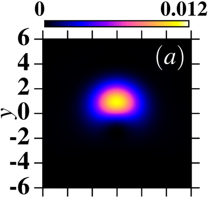
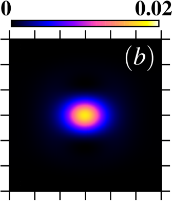
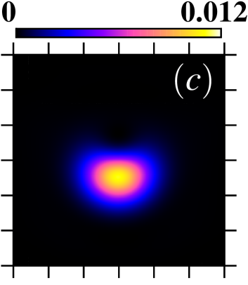
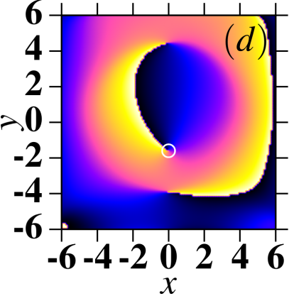
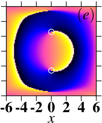
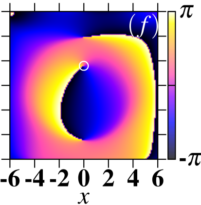
Figure 9: The 2D contour plots of densities of components in $z=0$ plane, corresponding to isodensity contours shown in 8, for (a) $m_{f}=+1$, (b) $m_{f}=0$, (c) $m_{f}=-1$ components of a moving vortex-bright soliton with $c_{0}=-10,$ $c_{1}=0.1$, $\gamma=1$, and $v=0.01$ towards positive $x$ direction. The corresponding phases are shown in (d) for $m_{f}=+1$, (e) for $m_{f}=0$, and (f) for $m_{f}=-1$ components.

Notwithstanding these qualitative similarities, there is a crucial difference. The moving vortex-bright soliton does not have the innumerable degenerate counterparts like the asymmetric vortex-bright soliton. This is due the fact that the system is no longer invariant under transformations: $\phi\rightarrow\phi+\delta\phi$ and $\psi_{m_{f}}(r,\theta,\phi)\rightarrow\psi_{m_{f}}(r,\theta,\phi+\delta\phi)e^{-im_{f}\delta\phi}$ due to the presence of $v$-dependent terms in Eqs. (IV.3)-(36). However, the system is invariant under transformations: $\phi\rightarrow\phi+\pi$ and$\psi_{m_{f}}(r,\theta,\phi)\rightarrow\psi_{m_{f}}(r,\theta,\phi+\pi)e^{-im_{f}\pi},v\rightarrow-v$. This transformation basically transforms a right moving vortex-bright soliton to its degenerate left moving counterpart. For $c_{0}=-10,$ $c_{1}=0.1$, and $\gamma=1$, the self-trapped solutions of Eqs. (IV.3)-(36) exist for $v\leq 0.04$.

V Summary

We have studied the formation and dynamics of 3D vortex-bright solitons in a three-component SO-coupled spin-1 spinor condensate using variational approximation and numerical solution of the mean-field GP equation. The solitons are metastable for $a_{0}+2a_{2}<0$ (predominantly attractive) and could be stable for $a_{0}+2a_{2}>0$ (predominantly repulsive). The ground state vortex-bright solitons are axisymmetric of type $(-1,0,+1)$ in the polar domain, whereas they are fully asymmetric in the ferromagnetic domain below a critical strength of spin-exchange interaction. In the latter case, the axisymmetric $(-1,0,+1)$ vortex-bright solitons are the excited states. The asymmetric vortex-bright solitons cannot appear in the polar domain. In addition, one can have $(0,+1,+2)\equiv(-2,-1,0)$ vortex-bright solitons as excited states in both domains. We demonstrate the dynamical stability of the solitons numerically. The present mean-field model is not Galelian invariant, and we study moving vortex-bright solitons using a Galilean-transformed model. The solitons can move without deformation.

- (1) Y. S. Kivshar and B. A. Malomed, Rev. Mod. Phys. 61, 763 (1989); F. K. Abdullaev, A. Gammal, A. M. Kam- chatnov, and L. Tomio, Int. J. Mod. Phys. B 19, 3415 (2005).
- (2) S. Inouye et al., Nature (London) 392, 151 (1998).
- (3) K. E. Strecker, G. B. Partridge, A. G. Truscott, and R. G. Hulet, Nature (London) 417, 150 (2002); L. Khaykovich, F. Schreck, G. Ferrari, T. Bourdel, J. Cubizolles, L. D. Carr, Y. Castin, and C. Salomon, Science 256, 1290 (2002).
- (4) S. L. Cornish, S. T. Thompson, and C. E. Wieman, Phys. Rev. Lett. 96, 170401 (2006).
- (5) V. M. Pèrez-Garc̀ia and J. B. Beitia, Phys. Rev. A 72, 033620 (2005); S. K. Adhikari, Phys. Lett. A 346, 179 (2005); Phys. Rev. A72, 053608 (2005); L. Salasnich and B. A. Malomed, Phys. Rev. A 74, 053610 (2006).
- (6) J. Ieda, T. Miyakawa, and M. Wadati, Phys. Rev. Lett. 93, 194102 (2004); L. Li, Z. Li, B. A. Malomed, D. Mihalache, and W. M. Liu, Phys. Rev. A 72, 033611 (2005); W. Zhang, Ö. E. Müstecaplioǧlu, and L. You, Phys. Rev. A 75, 043601 (2007); B. J. Dąbrowska-Wüster, E. A. Ostrovskaya, T. J. Alexander, and Y. S. Kivshar, Phys. Rev. A 75, 023617 (2007); E. V. Doktorov, J. Wang, and J. Yang, Phys. Rev. A 77, 043617 (2008); B. Xiong and J. Gong; Phys. Rev. A 81, 033618 (2010); P. Szankowski, M. Trippenbach, E. Infeld, and G. Rowlands, Phys. Rev. Lett. 105, 125302 (2010).
- (7) Y. Li, Giovanni I. Martone, and S. Stringari, Annual Review of Cold Atoms and Molecules, Vol. 3, (World Scientific, 2015), 201-250; V. Galitski and I. B. Spielman, Nature 494, 49 (2013).
- (8) K. Osterloh, M. Baig, L. Santos, P. Zoller, and M. Lewenstein, Phys. Rev. Lett. 95, 010403 (2005); J. Ruseckas, G. Juzeliūnas, P. Öhberg, and M. Fleischhauer, Phys. Rev. Lett. 95, 010404 (2005); G. Juzeliūnas, J. Ruseckas, and J. Dalibard, Phys. Rev. A 81, 053403 (2010); Z. Lan and P. Öhberg, Rev. Mod. Phys. 83, 1523 (2011).
- (9) Y.-J. Lin , K. Jiménez-García, and I. B. Spielman, Nature 471, 83 (2011).
- (10) Y. A. Bychkov E. I. Rashba, J. Phys. C 17, 6039 (1984).
- (11) G. Dresselhaus, Phys. Rev. 100, 580 (1955).
- (12) D.L. Campbell, R.M. Price, A. Putra, A. Valdés-Curiel, D. Trypogeorgos, and I.B. Spielman, Nature Commun 7, 10897 (2016).
- (13) M. Aidelsburger, M. Atala, and S. Nascimbene et al., Phys. Rev. Lett. 107, 255301 (2011); Z. Fu, P. Wang, and S. Chai, L. Huang, and J. Zhang, Phys. Rev. A 84, 043609 (2011); J.-Y. Zhang, S.-C. Ji, Z. Chen, L. Zhang, Z.-D. Du, B. Yan, G.-S. Pan, B. Zhao, Y.-J. Deng, H. Zhai, S. Chen, and J.-W. Pan, Phys. Rev. Lett. 109, 115301 (2012); C. Qu, C. Hamner, M. Gong, C. Zhang, and P. Engels, Phys. Rev. A 88, 021604(R) (2013).
- (14) Y. Xu, Y. Zhang, and B. Wu, Phys. Rev. A 87, 013614 (2013).
- (15) L. Salasnich, A. Parola, and L. Reatto, Phys. Rev. A 65, 043614 (2002).
- (16) L. Salasnich and B. A. Malomed, Phys. Rev. A 87, 063625 (2013); L. Salasnich, W. B. Cardoso, and B. A. Malomed, Phys. Rev. A 90, 033629 (2014); S. Cao, C.-J. Shan, D.-W. Zhang, X. Qin, and J. Xu, J. Opt. Soc. Am. B 32, 201 (2015).
- (17) H. Sakaguchi, B. Li, and B. A. Malomed, Phys. Rev. E 89, 032920 (2014); H. Sakaguchi and B. A. Malomed, Phys. Rev. E 90, 062922 (2014).
- (18) Y.-C. Zhang, Z.-W. Zhou, B. A. Malomed, and H. Pu, Phys. Rev. Lett. 115, 253902 (2015).
- (19) Y.-K. Liu and S.-J. Yang, Eur. Phys. Lett., 108, 30004 (2014).
- (20) S. Gautam and S. K. Adhikari, Laser Phys. Lett. 12, 045501 (2015).
- (21) S. Gautam and S. K. Adhikari, Phys. Rev. A 91, 063617 (2015).
- (22) S. Gautam and S. K. Adhikari, Phys. Rev. A 95, 013608 (2017).
- (23) T. Ohmi, and K. Machida, J. Phys. Soc. Japan, 67, 1822 (1998); T. L. Ho, Phys. Rev. Lett. 81, 742 (1998).
- (24) V. M. Perez-Garcia, H. Michinel, and H. Herrero, Phys. Rev. A57, 3837 (1998).
- (25) S. Gautam and S. K. Adhikari, Phys. Rev. A93, 013630 (2016); Phys. Rev. A 92, 023616 (2015); Phys. Rev. A 91, 013624 (2015); Phys. Rev. A 90, 043619 (2014).
- (26) T. Mizushima, K. Machida, and T. Kita, Phys. Rev. Lett. 89, 030401 (2002); Phys. Rev. A 66, 053610 (2002).
- (27) H. Zhai, Int. J. of Mod. Phys. B, 26, 1230001 (2012).
- (28) Y. Kawaguchi and M. Ueda, Phys. Rep. 520, 253 (2012).
- (29) P. Muruganandam and S. K. Adhikari, J. Phys. B 36, 2501 (2003).
- (30) H. Wang, J. Comput. Phys., 230, 6155 (2011); 274, 473 (2014).
- (31) W. Bao and F. Y. Lim, Siam J. Sci. Comp. 30, 1925 (2008); F. Y. Lim and W. Bao, Phys. Rev. E 78, 066704 (2008).
- (32) P. Muruganandam and S. K. Adhikari, Comput. Phys. Commun. 180, 1888 (2009); D. Vudragović, I. Vidanović, A. Balaž, P. Muruganandam, and S. K. Adhikari, Comput. Phys. Commun. 183, 2021 (2012); L. E. Young-S., D. Vudragovic, P. Muruganandam, S. K. Adhikari, and A. Balaž, Comput. Phys. Commun. 204, 209 (2016); B. Satarić, V. Slavnić, A. Belić, A. Balaž, P. Muruganandam, and S. K. Adhikari, Comput. Phys. Commun. 200, 411 (2016); R. Kishor Kumar, L. E. Young-S., D. Vudragovič, Antun Balaž, P. Muruganandam, S. K. Adhikari, Comput. Phys. Commun. 195, 117 (2015); V. Loncar, L. E. Young-S., S. Skrbic, P. Muruganandam, S. K. Adhikari, A. Balaž, Comput. Phys. Commun. 209, 190 (2016); V. Loncar, A. Balaž, A. Bogojevic, S. Skrbic, P. Muruganandam, S. K. Adhikari, Comput. Phys. Commun. 200, 406 (2016).
- (33) J.-P. Martikainen, Dynamics and excitations of Bose-Einstein condensates, Acedemic dissertation, Helsinki Institute of Physics, University of Helsinki (2001).
- (34) G. I. Martone, Y. Li, and S. Stringari Phys. Rev. A 90, 041604(R) (2014).