A quantum analogue to the deflection function

Abstract

The classical deflection function is a valuable computational tool to investigate reaction mechanisms. It provides, at a glance, detailed information about how the reaction is affected by changes in reactant properties (impact parameter) and products properties (scattering angle), and, more importantly, it also shows how they are correlated. It is also useful to predict the presence of quantum phenomena such as interferences. However, rigorously speaking, there is not a quantum analogue as the differential cross section depends on the coherences between the different values of $J$ caused by the cross terms in the expansion of partial waves. Therefore, the classical deflection function has a limited use whenever quantum effects become important. In this article, we present a method to calculate a quantum deflection function that can shed light onto reaction mechanism using just quantum mechanical results. Our results show that there is a very good agreement between the quantum and classical deflection function as long as quantum effects are not all relevant. When this is not the case, it will be also shown that the quantum deflection function is most useful to observe the extent of quantum effects such as interferences. The present results are compared with other proposed quantum deflection functions, and the advantages and disadvantages of the different formulations will be discussed.

I Introduction

The main goal of reaction dynamics is to obtain the various microscopical properties as excitation functions or rotational distributions and from them, macroscopical properties such as thermal rate coefficients. Overall, the process is equivalent to disentangling how microscopical properties govern the macroscopic outcome. Accordingly, it is not enough to reproduce and predict experimental measurements, but it is also important to unveil the detailed reaction mechanisms.

Impact parameter $b$ (or orbital angular momentum $\bm{\ell}$) and scattering angle $\theta$ are two of the main variables that are studied to discern reaction mechanisms. The former is related to the reactants asymptote, and is one of the key players in determining the outcome of a collision Levine (2005); by M. Brouard and Vallance (2010) as it determines the parts of the potential energy surface (PES) that will be explored during the collision (head-on vs. glacing collisions). The scattering angle, in turn, is defined at the product asymptote and provides information about nuclei scrambling during the collision; besides, it is amenable of experimental measurement using cross molecular beams with mass spectrometric universal detection or, more recently, velocity-mapped ion imaging Eppink and Parker (1997); Gijsbertsen et al. (2005); Lin et al. (2003); Ashfold et al. (2006) or single beam coexpansion such as photoloc Schafer et al. (1993) among other techniques. Moreover, it is relatively straightforward to extract the reaction (or inelastic) probability as a function of $J$ (opacity function or $P_{r}(J)$), and the differential cross section (DCS) as a function of the scattering angle $\theta$. Hence, it is not surprising that $P_{r}(J)$ and DCS are two of the most important observables in reaction dynamics.

The deflection function, that is, is the joint dependence of the reaction probability as a function of the scattering angle and the impact parameter, contains all the information provided by the $P_{r}(J)$ and the DCS and, above all, how $J$ and $\theta$ correlate throughout the collision. The classical deflection function has been widely used to explain elastic and inelastic scattering, in particular to understand those features related with glory and rainbow scattering Ford and Wheeler (1959); Berstein (1966); Levine (2005). For reactive scattering a strong correlation between $J$ and $\theta$ is expected for reactions following a direct mechanism, whereas none or very weak correlation between these variables can be anticipated if the reaction takes place through a long-lived collision complex. Furthermore, discontinuities and different trends in the deflection function can be used to characterized different reaction mechanism even for apparently simple reactionsGreaves et al. (2008, 2008).

The classical deflection function has been also used to predict interferences causing oscillations in the DCS. Given the wave nature of quantum mechanics (QM), it is expected that when one particle may follow two different pathways giving rise to the same outcome, they will interference. In the double-slit Young experiment Feynman et al. (1970) interferences arise when electrons going through two different slits could hit the detector. In reaction dynamics we do not need slits and the system itself acts as an interferometer whenever two different $J$ could scatter at the same angles Jambrina et al. (2015, 2016); Sneha et al. (2016). This analogy also explains why the deflection function cannot be calculated using pure quantum mechanical grounds in the same way as it is done in classical calculations. In quantum mechanics, the angular distribution depends on the coherences between different $J$-partial waves, therefore something apparently as simple as obtaining a rigorous joint probability distribution as a function of $J$ and $\theta$ cannot be computed. That would be similar to disentangle which parts of the signal comes from electrons going through one or other slit in the Young double-slit experiment.

It is not surprising that many efforts have been done to overcome this limitation. Especially interesting is the so-called Quantum Deflection Function (CQDF) devised by Connor and coworkers Connor (2004); Shan and Connor (2011); Xiahou and Connor (2009) in the context of the glory analysis of forward scattering. The CQDF, defined as the derivative of the argument of the scattering matrix element with respect to $J$, has probed to be a valuable tool to predict the presence of rainbows and to identify the rainbow angular momentum variable. Besides, it could be used to predict interferences between nearside and farside scattering. However, CQDF provides a single value of $\theta$ (actually, of the deflection angle, $\Theta$, whose absolute value is the measurable scattering angle $\theta$) for one or few $J$s so it cannot be considered as a joint probability of $J$ and $\theta$. Moreover, the CQDF does not consider that a single $J$ can correlate with a continuous series of different $\theta$ which impairs its use to predict the presence of different mechanisms.

Throughout this article, we will try to circumvent this limitation, and we will propose a new quantum analogue to the classical deflection function, $Q_{r}(\theta,J)$ or QM-DF, which may be useful for the interpretation of quantum scattering results. This new function is a sort of joint distribution of $J$ and $\theta$ that includes all coherences between different partial waves, and whose summation over all partial waves recovers the exact angular distribution. The article is organized as follows: in Section II we will revise the classical deflection function as the joint distribution of $\theta$ and $J$, followed by the definition of a intuitively simple QM-DF, $Q_{r}(\theta,J)$, starting from the definition of the scattering amplitude, that will be compared with the QCT deflection function. In Section III we will assay the validity and usefulness of the proposed QM-DF for three different systems and situations. First of all, we will study the inelastic collisions of Cl + H₂, where the QCT deflection function succeeded in explaining the quantum results. Next, we will study the reactive D⁺ + H₂ system, prototype of barrierless reactions where we expect no correlation between $J$ and $\theta$. Finally, we will apply the QM-DF to reactive scattering between H and D₂ at high collision energies where quantum interferences govern the angular distributions for certain combinations of final and initial states. For all these systems, QM calculations have been carried out using the close-coupling hypespherical method of Skouteris et al. Skouteris et al. (2000), while QCT calculations have been performed using the procedure described in Refs. 20 and 21.

II Theory

II.1 Classical Deflection Function

The basis of the QCT method consists in calculating an ensemble of trajectories following a judicious sampling of initial conditions to cover as much as possible the phase space relevant for the process to be studied but complying with the state quantization of the reactants. The initial and final atom positions and linear momenta are then used to determine those initial and final properties (such as angular momenta, scattering angle, final states, etc.) necessary to characterize each individual trajectory. Finally, all is needed is to carry out the average value of any conceivable property over the ensemble of trajectories. For example, the total reaction probability for a given value of the total angular momentum quantum number, $J$, discretely sampled can be obtained as:

$$P_{r}(J)=\frac{N_{r}(J)}{N_{\rm tot}(J)}$$ (1)

where $N_{r}(J)$, and $N_{\rm tot}(J)$ are the number of reactive (or inelastic if that were the case) and total trajectories, respectively, for a given $J$. Recall that the total angular momentum $\bm{J}=\bm{\ell}+\bm{j}$, where $\bm{j}$ is the rotational angular momentum and $\bm{\ell}$ is the (relative) orbital angular momentum. We can define the corresponding quantum numbers, $J$, $\ell$ and $j$, such that ${|\bm{J}|=[J(J+1)]^{1/2}\hbar}$ and similarly for $|\bm{\ell}|$ and $|\bm{j}|$. These quantum numbers can be sampled continuously (real values) or discretely (integer values).

Equation (1) is valid if the sampling in $J$ is discretely and uniformly sampled and, similarly, for the orbital angular momentum in the $|J-j|\leq\ell\leq J+j$ interval (for details see ref. 22). In addition, not all reactive trajectories need to have the same weight. Sometimes it is necessary to attribute different weights to each trajectory as is done in the Gaussian binning procedureBonnet and Rayez (1997); Bañares et al. (2003); Bonnet and Rayez (2004) to make the assignment of final rovibrational states ‘more quantal’, or simply because a biased sampling is used. In those cases, $N_{r}(J)$ in Eq. (1) is replaced by $S_{w}$, the sum of the weights of reactive (or inelastic) trajectories into a given final manifold of states. If one wishes to calculate a property that depends on more than one variable, for example of $J$ and $\ell$, the scheme is the same except that now a joint probability has to be considered (say, the number of reactive trajectories with values of $J$ and $\ell$, $N_{r}(J,\ell)$).Aoiz et al. (2005) The aforementioned procedure is suitable for discrete variables, while for continuous variables it is a common practice to use histograms or, more elegantly, to fit the distributions to series of orthogonal polynomials. Aoiz et al. (1992, 1998, 2005) Obviously, integration (or summation) over one of the variables of a given joint probability distribution, leads to the probability distribution of the other variable. Moreover, if we split the original ensemble of trajectories in a series of sub-ensembles and calculate the respective joint probability distribution, it turns out that the global probability distribution can be easily recovered from the joint probabilities distributions for all the sub-ensembles; that is to say, the probability distributions are always additive. As we will see, this is not the case in QM scattering due to the interferences.

To illustrate the calculation of the classical deflection function, let us assume that the orbital angular momentum is sampled continuously in the ${\ell\in[0,\ell_{\max}]}$ with a weight $2\ell+1$, that is, the orbital angular momentum for the $i$-th trajectory is sampled as $\ell_{i}(\ell_{i}+1)=\xi_{i}[\ell_{\max}(\ell_{\max}+1)]$, where $\xi$ is a random number in $[0,1]$ (this is the same as sampling the impact parameter as $b=\xi^{1/2}b_{\max}$).

We can conveniently define a $J$-partial cross section, $\sigma_{r}(J)$:

$$\sigma_{r}(J)=\frac{\pi}{k^{2}}\,(2J+1)\frac{2\min(J,j)+1}{2j+1}P_{r}(J)\,,$$ (2)

which is nothing but a probability density function normalized such that the integral or the sum of $\sigma_{r}(J)$ over $J$ is the integral cross section, $\sigma_{r}$, either total or into a given final state.Aoiz et al. (2005) For discrete values of $J$, $\sigma_{r}(J)$ is usually denoted in the literature as $\sigma_{r}^{J}$.

The Monte Carlo normalized probability density function can be written as

$$\sigma_{r}(J)=\frac{\sigma_{r}}{S_{w}}\,\sum_{i=1}^{N_{r}}w_{i}\delta(J-J_{i})\,,$$ (3)

where $w_{i}$ and $J_{i}$ are the weight and $J$ value of the $i$-th trajectory. $S_{w}$ is the sum of the weights of all the relevant reactive trajectories, $S_{w}=\sum w_{i}$. In the simplest case, $w_{i}$ would be a Boolean function whose value is one only for the specific reactive trajectories and zero otherwise, such that $S_{w}=N_{r}$, the number of the considered reactive trajectories. As a convenient approximation, the Dirac delta functions can be replaced with a normalized Gaussian function

$$G(J-J_{i})=\frac{1}{s\sqrt{\pi}}\exp\left[-\frac{(J-J_{i})^{2}}{s^{2}}\right]\,,$$ (4)

where the width, $s=\Delta_{\rm FWHM}/\ln 2$, is conveniently chosen depending on the average spacing of the successive values of $J_{i}$ and the statistical uncertainty.

If the sampling in $J$ (and in $\ell$) is made continuous, the $J$-partial cross section can be expressed as an expansion in Legendre polynomials, $P_{n}(x)$:

$$\sigma_{r}(J)=\sigma_{r}\,\,\frac{2(2J+1)}{J_{\max}(J_{\max}+1)}\,\sum_{n}b_{n}P_{n}[x(J)]\,,$$ (5)

where $x$ is a reduced variable, $x\in[-1,1]$, given by

$$x=\frac{J(J+1)}{J_{\max}(J_{\max}+1)}-1\,,$$ (6)

where $J_{\max}$ is the maximum value of the total angular momentum used in the calculation to ensure the convergence. The coefficients, $b_{n}$, are given in terms of the Legendre moments as

$$b_{n}=\frac{2n+1}{2}\,S_{w}^{-1}\,\sum_{i=1}^{N_{r}}w_{i}\,P_{n}(x_{i})\,,$$ (7)

where $x_{i}$ is the value of $x$, given by Eq. (6), of the i-th trajectory, and $P_{n}(x)$ is the n-th order Legendre polynomial.

Similarly, the DCS can be expressed as an expansion in Legendre polynomials:

$$\sigma_{r}(\theta)\equiv\frac{d\sigma(\theta)}{d\omega}=\frac{\sigma_{r}}{2\pi}\,\sum_{m=0}a_{m}P_{m}(\cos\theta),$$ (8)

where $\sigma_{r}$ is the integral cross section, and $a_{n}$ are the expansion coefficients whose values are given by:

$$a_{m}=\frac{2m+1}{2}\langle P_{m}(\cos\theta)\rangle=\frac{2m+1}{2}\,S_{w}^{-1}\,\sum_{i=1}^{N_{r}}w_{i}P_{n}(\cos\theta_{i})\,,$$ (9)

where $\langle P_{m}(\cos\theta)\rangle$ is the weighted average value of $P_{m}(\cos\theta)$ over the ensemble of the relevant trajectories.

The classical deflection function, that is, the joint probability distribution of $J$ and $\theta$, normalized to the integral cross section, can now be expressed as a double expansion in Legendre polynomials

$$\sigma_{r}(\theta,J) = \frac{\sigma_{r}}{2\pi}\,\frac{2(2J+1)}{[J_{\max}(J_{\max}+1)]}\sin\theta\,\cdot$$

$$\sum_{m=0}\,\sum_{n=0}\alpha_{mn}P_{m}(\cos\theta)P_{n}[x(J)]$$

where the coefficients $\alpha_{mn}$ are given by:

$$\alpha_{mn} =\frac{(2m+1)(2n+1)}{4}\langle P_{m}(\cos\theta)P_{n}[x(J)]\rangle=$$

$$\frac{(2m+1)(2n+1)}{4}S_{w}^{-1}\sum_{i=1}^{N_{r}}w_{i}P_{m}(\cos\theta_{i})P_{n}[x_{i}(J_{i})]$$

The Monte Carlo expression of the deflection function can be expressed as a sum of Gaussian functions given by

$$\sigma_{r}(\theta,J) =\frac{\sigma_{r}}{2\pi}\,S_{w}^{-1}~{}\sum_{i=1}^{N_{r}}w_{i}\,\delta(J-J_{i})\delta(\theta-\theta_{i})\approx$$ (12)

$$\frac{\sigma_{r}}{2\pi}\,S_{w}^{-1}~{}\sum_{i=1}^{N_{r}}w_{i}\,G(J-J_{i})G(\theta-\theta_{i})$$

where $J_{i}$ and $\theta_{i}$ represent the values of $J$ and $\theta$ for the $i$-th trajectory. $G(J-J_{i})$ and $G(\theta-\theta_{i})$ denote normalized Gaussian functions with width parameters $s_{{}_{J}}$ and $s_{\theta}$, centred in $J_{i}$ and $\theta_{i}$, respectively.

Integration of Eq. (II.1) or Eq. (12) over $\theta$ and the azimuthal angle renders the $J$-partial cross section of Eq. (5) and Eq. (3). Alternatively, integration over $J$ in those equations gives the $\sigma_{r}(\theta)\,\sin\theta$.

II.2 QM analogue to the Deflection Function

Due to its classical nature, there is no restriction in QCT calculations to obtain any correlation between two or more properties. After all, each trajectory is characterized by specific values of any initial or final property. However, this is not the case for QM scattering calculations, which makes the analysis based on pure QM calculations not so trivial. From the QM scattering calculations we only obtain as an outcome the scattering matrix (S-matrix) that relates the initial states of the reactants and the final states of the products. In the unsymmetrized representation, the S-matrix has one element per energy, chemical rearrangement $\alpha$, $J$, and initial and product states. For the particular case of closed shell diatomic molecules in the helicity representation (body-fixed frame), and a given value of $J$, these are characterized by three quantum numbers for each arrangement: $v$, $j$, ($v^{\prime}$ and $j^{\prime}$) that define the vibrational and rotational states respectively, and the helicity $\Omega$ ($\Omega^{\prime}$), the projection of $\bm{j}$ ($\bm{j}^{\prime}$) (or $\bm{J}$) onto the approach (or recoil) direction. It means that to obtain a dynamical observable from a QM calculation, we need a recipe to extract its value from the elements of the S-matrix.

Some observables can be readily extracted from the S-matrix. This is the case of the $P_{r}(J;E)$ that, for a given initial state and total energy, can be calculated as follows:

$$P_{r}(J;E)=\frac{1}{2\min(J,j)+1}\,\,\sum_{\Omega}\sum_{\Omega^{\prime}}\left|S^{J\alpha}_{v^{\prime}j^{\prime}\Omega^{\prime},vj\Omega}(E)\right|^{2}$$ (13)

where the sum runs over the desired products states (or, if referred to state-to-state, without summing over $v^{\prime}$ and $j^{\prime}$). Hereinafter, subscripts for the $v$, $j$, $v^{\prime}$, $j^{\prime}$, energy, and the chemical arrangement will be omitted for clarity. The integral cross section can be written in terms of the reaction probabilities as

$$\sigma_{r}(E) = \frac{\pi}{k_{vj}^{2}}\,\sum_{v^{\prime},j^{\prime}}\,\sum_{J=0}^{J_{\max}}(2J+1)\,\frac{2\min(J,j)+1}{j+1}\,\,P_{r}(J;E)=$$ (14)

$$\sum_{J=0}^{J_{\max}}(2J+1)\,\sigma_{r}^{J}(E)$$

where $k^{2}_{vj}=2\mu(E-E_{vj})/\hbar^{2}$, is the initial relative wavenumber vector, and $\mu$ is the atom-diatom reduced mass. $J_{\max}$ is the maximum value of $J$ necessary for convergence. $\sigma_{r}^{J}(E)$ is the $j$-partial cross section already mentioned in the previous subsection.

To extract vector properties such as the DCS from the S-matrix is not so straightforward. First, because we need to include the angular dependence; second, because they involve coherences between different elements of the S-matrix. It is convenient to express the DCS in terms of the scattering amplitudes, which are defined as:

$$f_{\Omega^{\prime}\Omega}(\theta)=\frac{1}{2\imath k_{vj}}\sum_{J=0}^{J_{\rm max}}(2J+1)d^{J}_{\Omega^{\prime}\Omega}(\theta)S^{J}_{\Omega^{\prime},\Omega}$$ (15)

where $d^{J}_{\Omega^{\prime}\Omega}(\theta)$ is the Wigner d-matrix. The DCS can now be written using the scattering amplitudes as:

$$\sigma_{r}(\theta)\equiv\frac{d\sigma_{r}(\theta)}{d\omega}=\frac{1}{2j+1}\sum_{\Omega^{\prime}\Omega}f^{*}_{\Omega^{\prime}\Omega}(\theta)f_{\Omega^{\prime}\Omega}(\theta)$$ (16)

From Eqs. (15) and Eq. (16) it is clear that the DCSs for state-to-state processes are additive, even when they are resolved in $\Omega^{\prime}$, and $\Omega$. However, the squaring of the sum over $J$ in Eq. 15 makes the DCS no longer additive in $J$. This property is a reflection of the wave nature of quantum mechanics, so that two “paths” (impact parameters or $J$) leading to scattering at the same angles interfere. Hence, in principle, it is not possible to separate the contribution of two mechanisms (or paths) in a overall DCS. It is worth noticing that usually the interference are only important between nearby values of $J$ Panda et al. (2012) so, for certain cases, it is possible to extract the contributions from one or many mechanisms from the DCS.

To calculate a QM deflection function we would need to extract the contribution of each $J$ to the total DCS. Furthermore, to be reliable and to provide a valuable insight into the collision mechanism, the QM deflection function should be additive, so that the sum over $J$ should be enough to recover the overall DCS. One could, in principle, compute it by neglecting all coherences between different $J$s. This would be equivalent of using the random phase approximation that lies in the core of the statistical model Rackham et al. (2003, 2001), giving rise to forward-backward symmetric DCSs. For non-statistical (direct) reactions, a symmetric DCS is in clear disagreement with the experimental results, and hence neglecting coherences can be considered as a very unappropriate approximation to obtain a QM deflection function. To devise a QM analogue to the deflection function we will start by defining a $J$-partial dependent scattering amplitude as:

$$f^{J}_{\Omega^{\prime}\Omega}(\theta)=\frac{1}{2ik_{vj}}\,(2J+1)d^{J}_{\Omega^{\prime}\Omega}(\theta)S^{J}_{\Omega^{\prime}\Omega}$$ (17)

where $|\Omega|,~{}|\Omega^{\prime}|\leq J$. The (total) scattering amplitude can now be written as

$$f_{\Omega^{\prime}\Omega}(\theta)=\sum_{J=0}^{J_{\rm max}}f^{J}_{\Omega^{\prime}\Omega}(\theta)$$ (18)

The DCS can be expressed as a function of the $J$-partial scattering amplitudes:

$$\sigma_{r}(\theta)=\frac{1}{2j+1}\sum_{\Omega^{\prime}\Omega}~{}\sum_{J_{1}=0}^{J_{\max}}\sum_{J_{2}=0}^{J_{\max}}f^{J_{1}}_{\Omega^{\prime}\Omega}(\theta)f^{J_{2}*}_{\Omega^{\prime}\Omega}(\theta)\,,$$ (19)

which is the same as Eq. (16). Without any approximation, Eq. 19 can be rearranged to

$$\sigma_{r}(\theta) = \frac{1}{(2j+1)}\sum_{\Omega^{\prime}\Omega}~{}\sum_{J=0}^{J_{\rm max}}{\ }\sum_{J_{1}=0}^{J_{\max}}\sum_{J_{2}=0}^{J_{\max}}\,\frac{\left(\delta_{J_{1},J}+\delta_{J_{2},J}\right)}{2}\cdot$$ (20)

$$f^{J_{1}}_{\Omega^{\prime}\Omega}(\theta)f^{J_{2}*}_{\Omega^{\prime}\Omega}(\theta).$$

Eqs. (19) and (20) only differ in the presence of an additional sum over $J$ in (20) that is compensated with the term $(\delta_{J_{1},J}+\delta_{J_{2},J})/2$, that guarantees that both equations include the same number of cross products and hence that they are equivalent. The advantage of Eq. (20) is the presence of a separate summation over $J$ that allows us to define a function that depends on a single $J$ and $\theta$; that is, a quantum analogue to the classical deflection function (QM-DF) that we will denote as $Q_{r}(\theta,J)$,

$$Q_{r}(\theta,J) = \frac{\sin\theta}{2j+1}\,\sum_{\Omega^{\prime}\Omega}~{}\sum_{J_{1}=0}^{J_{\max}}\sum_{J_{2}=0}^{J_{\max}}\,\frac{\left(\delta_{J_{1},J}+\delta_{J_{2},J}\right)}{2}\cdot$$ (21)

$$\,\,f^{J_{1}}_{\Omega^{\prime}\Omega}(\theta)f^{J_{2}*}_{\Omega^{\prime}\Omega}(\theta)\,.$$

To help the interpretation of the quantum deflection function defined in this work, Eq. (21) can be recast as

$$Q_{r}(\theta,J) = \frac{\sin\theta}{2j+1}\,\sum_{\Omega^{\prime}\Omega}~{}|f^{J}_{\Omega^{\prime}\Omega}|^{2}\cdot$$ (22)

$$+ \frac{1}{2}\,\sum_{\Omega^{\prime}\Omega}\sum_{\begin{subarray}{c}J_{1}=0\\ J_{1}\neq J\end{subarray}}^{J{\max}}\,\left[f^{J}_{\Omega^{\prime}\Omega}(\theta)f^{J_{1}*}_{\Omega^{\prime}\Omega}(\theta)+~{}\text{c.c.}\right]\,.$$

where c.c. stands for the respective conjugate complex. Equation (22) contains the square of the $J$-dependent scattering amplitude, $|f^{J}_{\Omega^{\prime}\Omega}(\theta)|^{2}$, plus a halved summation of $J_{\max}$ terms over all the total angular momenta $J_{1}\neq J$, which are the coherent terms. The other half of the summation will appear in previous or subsequent values of $J$. In the absence of coherences, that is, in the random phase approximation limit, the only surviving term would be that depending of $J$ only. The remaining terms account for the possible interferences that most of the time can be expected to be only important between partial waves in a restricted range of $J$ in $[J-\Delta J,J+\Delta J]$.Jambrina et al. (2015, 2016) However, as it will be shown below, interferences can also take place between partial waves that cover the full range of angular momentum leading to scattering.

The QM-DF shares some important properties in common with the classical ones. As in the classical case, summing Eq. (21) over $J$ leads to the DCS given by Eq. (20) multiplied by $\sin\theta$, $\sigma_{r}(\theta)\sin\theta$. Similarly, by integration over the scattering angle and the azimuthal angle,

$$\int_{-1}^{1}{\rm d}\theta~{}~{}Q_{r}(\theta,J)=\frac{\pi}{k^{2}_{v,j}}\,\,\frac{2J+1}{2j+1}\sum_{\Omega^{\prime}\Omega}~{}|S^{J}_{\Omega^{\prime}\Omega}|^{2}=\sigma^{J}(E)\,,$$ (23)

gives the $J$-partial cross section, Eq. (14), as in the classical treatment.

In spite of the similarities between the classical $\sigma_{r}(\theta,J)$ (Eq. (II.1) or Eq. (12)) and the quantum $Q_{r}(\theta,J)$ (Eq. (21)) there are important differences and hence the qualifier “analogue”. The latter is not a genuine joint probability distribution (and, hence, a true deflection function in the classical sense) since it includes coherences between different values of $J$. Moreover, it can take negative values whenever there are destructive interferences between pairs of $J$ values, although when summed over $J$ a positive value is recovered. Notwithstanding the differences, as it will be shown in Section III, when the interferences are not significant, classical deflection functions and QM-DF bear a close resemblance.

It is sometimes useful to calculate the angular distributions for a subset of partial waves These angular distributions, labeled as DCS($J_{k}$-$J_{i}$) can be calculated by restricting the sum in Eq. (15) to a given range of $J$, $J\in[J_{i},J_{k}]$,

$$\sigma_{r}(\theta;J_{k}-J_{i})=\sum_{J=J_{i}}^{J_{k}}\sigma_{r}(J,\theta)$$ (24)

The partially summed DCS, $\sigma_{r}(\theta;J_{k}-J_{i})$, include all coherences between partial waves within the $[J_{i},J_{k}]$ range but none outside this range. In addition, like the DCS itself, $\sigma_{r}(\theta;J_{k}-J_{i})$ are not additive, especially if there are interferences between different groups of $J$s.

By analogy, it is also possible to define a deflection function by restricting the sum over a given $[J_{i},J_{k}]$ range of $J$, $Q_{r}(\theta;J_{k}-J_{i})$, as

$$Q_{r}(\theta;J_{k}-J_{i})=\sum_{J=J_{i}}^{J_{k}}Q_{r}(J,\theta)\,,\quad\text{with}~{}~{}J_{i}\leq J_{k}$$ (25)

In spite of the similarities between the partial $\sigma_{r}(\theta;J_{k}-J_{i})$ and $Q_{r}(\theta;J_{k}-J_{i})$ (and the fact that in the limit of the full interval, $J_{i}=0$ and $J_{k}=J_{\max}$, both functions are identical) there are two main differences between them: i) The latter also includes coherences between partial waves outside the $[J_{i},J_{k}]$ range so it may take negative values (if destructive interferences prevail for some scattering angles); ii) the deflection functions so defined, as in the classical case, are additive. Hence, from the comparison between the partially summed DCSs and partial QM-DFs it is easy to disentangle the presence and position of interference phenomena.

II.3 Other Quantum deflection functions

The idea of a semiclassical deflection function was first developed by Ford and Wheeler in the context of elastic scattering using the stationary phase approximation,Ford and Wheeler (1959) and later consolidated by Bernstein. Berstein (1966) The semiclassical approximation techniques proved to be very useful to gain insight into the the physical nature of scattering, making possible to extract qualitative inferences and easing the interpretation of the quantum results. Berstein (1966); Child (1996); Connor (1979)

The semiclassical deflection function, $\Theta(\ell_{\theta})$, is related to the phase shift, $\eta_{\ell}$ by

$$\Theta(\ell_{\theta})=2\,\left(\frac{{\rm d}\eta_{\ell}}{{\rm d}l}\right)_{\ell_{\theta}}$$ (26)

where $\Theta=\pm\theta$ for repulsive and attractive potentials, respectively, and the derivative of $\eta_{l}$ is evaluated at $\ell_{\theta}$, the $\ell$-value of the stationary phase. The phase shift can be written in terms of the $S$ matrix as

$$S_{\ell}=\mathrm{e}^{2i\eta_{\ell}}$$ (27)

hence,

$$\Theta(\ell)=\frac{{\rm d}}{{\rm d}\ell}\left[\arg S_{\ell}\right]$$ (28)

In a series of articles, Connor and co-workers extended the semiclassical treatment and developed a quantal version of the deflection function applicable to the most general case of inelastic or reactive scattering.Connor (2004); Shan and Connor (2011); Xiahou and Connor (2009) It is thus pertinent to compare our proposed QM-DF with that presented by Connor and coworkers (hereinafter denoted as CQDF). We have followed the procedure expounded in Ref. 16. In what follows, we will briefly summarize the main equations of that method for our present purposes.

For a given initial and final rovibrational states the CQDF, denoted as $\tilde{\Theta}_{\Omega^{\prime}\Omega}$, is defined as

$$\tilde{\Theta}_{\Omega^{\prime}\Omega}(J)=\frac{\,{\rm d}}{{\rm d}\,J}[\arg\tilde{S}_{\Omega^{\prime}\Omega}(J)]\,,$$ (29)

where $\tilde{S}_{\Omega^{\prime}\Omega}(J)$ is the modified scattering matrix elements that can be calculated directly from the scattering matrix:

$$\tilde{S}_{\Omega^{\prime}\Omega}(J)=\exp(\imath\pi J)S^{J}_{\Omega^{\prime}\Omega}$$ (30)

It should be highlighted that $\arg\tilde{S}_{\Omega^{\prime}\Omega}(J)$ does not denote the principal value, but it is defined as a continuous function as follows:

$$\arg\tilde{S}_{\Omega^{\prime}\Omega}(J)=\arctan\frac{{\rm Im}[\tilde{S}_{\Omega^{\prime}\Omega}]}{{\rm Re}[(\tilde{S}_{\Omega^{\prime}\Omega}]}+2n\pi$$ (31)

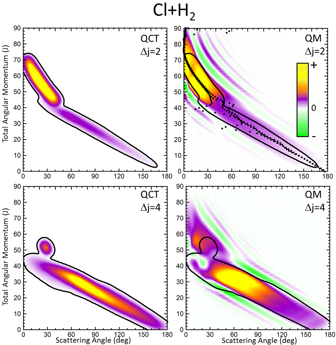
Figure 1: Comparison of the QCT deflection functions (left panels) and the analogue QM deflection function (right panels) for the Cl+H₂($v=0$, $j=0$) $\to$ Cl +H₂($v^{\prime}=0$, $j^{\prime}=2,4$) inelastic collisions at $E_{\rm col}=$0.73 eV. Top panels, $\Delta j$=2; bottom panels, $\Delta j$=4. The contour of the QCT deflection function has been added to the QM $Q_{r}$ to make the comparison easier. The green colour corresponds to negative value, hence destructive interferences ($Q_{r}(\theta,J)<0$). For comparison purposes, Connor’s QDF is shown on top of the QM analogue deflection function for $\Delta$j=2 using black dots.

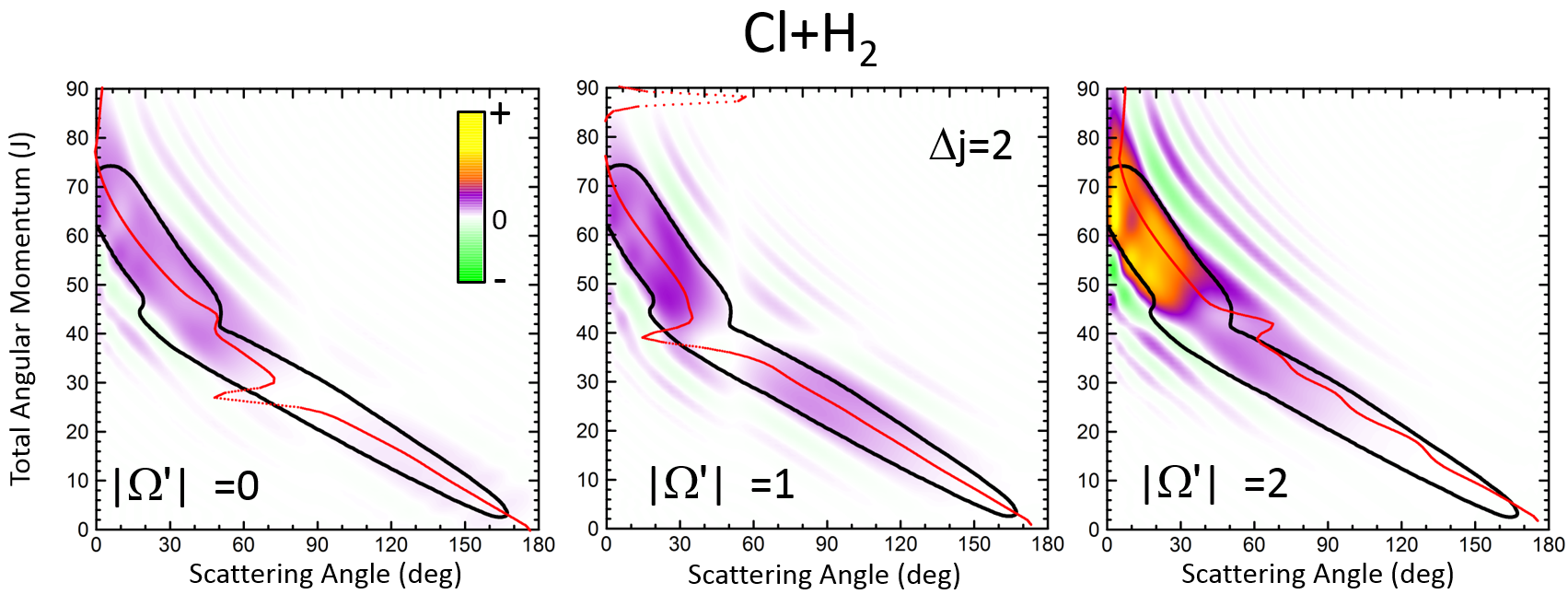
Figure 2: QM deflection function at $E_{\rm col}=$0.73 eV for the Cl+H₂($v=0$, $j=0$) $\to$ Cl +H₂($v^{\prime}=0$, $j^{\prime}=2$, $|\Omega^{\prime}|=0,1,2$) inelastic collisions resolved in $\Omega^{\prime}$ helicity states. The corresponding Connor’s QDF are also shown using solid red lines.

where $n$ is a positive or negative integer number, whose value is arbitrarily set to 0 for $J$=0, and for $J>$0 is selected such that $\arg\tilde{S}_{\Omega^{\prime}\Omega}(J)-\arg\tilde{S}_{\Omega^{\prime}\Omega}(J-1)<\pi$ is a continuous function. It should be emphasised that whilst $Q_{r}$ is a sort of a probability density function in terms of both $\theta$ and $J$, and therefore contains information about the scattering intensity and the presence of constructive or destructive interferences, CQDF represents a relation between the deflection angle (or the scattering angle) and the angular momentum $J$. Moreover, as shown in the previous subsection, if the present QM-DF is summed over over $J$, one gets the DCS. Another difference is that whilst CQDF is defined for each pair of $\Omega$ and $\Omega^{\prime}$ values, the QM-DF defined in this work can include the average over the reactant’s and the summation over product’s helicities as shown in Eq. (21), although it can be also calculated for specific values of $\Omega$ and $\Omega^{\prime}$, a it will be shown below. Apart from these differences, one would expect a confluence with regard to the relationship between scattering angle and angular momentum.

III Results and Discussion

III.1 Inelastic collisions between Cl and H₂

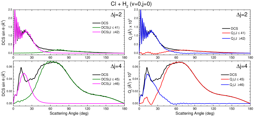
Figure 3: Comparison of the DCS partially summed over the indicated $J$ interval, $\sigma(\theta;J_{k}-J_{i})$ (defined in Eq. (24)), (left panels) and the QM deflection functions summed over the same $J$ intervals $Q_{r}(\theta;J_{k}-J_{i})$ (defined in Eq. (25))(right panels) for the inelastic collisions between Cl and H${}_{2}(v=0,j=0)$ at $E_{\rm col}=$0.73 eV and $\Delta j$=2 (top panels) and $\Delta j$=4 (bottom panels).

The first example in which we will use the QM-DF proposed in this work is the inelastic collisions between Cl and H${}_{2}(v=0,j=0)$. This system has been extensively studied both computacional and experimentally, Althorpe and Clary (2003); Alagia et al. (1996); Casavecchia (2000); Wang et al. (2008); Balucani et al. (2003) especially with regard to the role played by the spin-orbit interaction and non-adiabatic effects for the hydrogen exchange reaction.

As for inelastic collisions, some interesting features emerged in previous studies.Gonzalez-Sanchez et al. (2011); Aldegunde et al. (2012) QM and QCT calculations using the BW2 PES Bian and Werner (2000) showed that at relatively high collision energies ($E_{\rm coll}>0.6$ eV) and for small $\Delta j$ values ($\Delta j=j^{\prime}-j$), the inelastic probabilities, $P_{r}(J)$, exhibit two maxima separated by a minimum in the QCT and QM results. This minimum was identified as that corresponding to the glory impact parameter. The analysis of the results showed that there are two mechanisms responsible of the inelastic scattering resulting in very different stereodynamical behaviours, and associated to different regions of the PES.Gonzalez-Sanchez et al. (2011); Aldegunde et al. (2012) The two distinct dynamical regimes depend primarily on the value of the total (here also orbital) angular momentum: (i) for $J$s below the glory impact parameter, collisions seem to take place following a sort of “tug-of-war” mechanism Greaves et al. (2008) that implies the stretching of the H-H bond,Aldegunde et al. (2012); and (ii) for $J\gtrsim 40$ collisions can be assigned to rainbow scattering in which the attractive part of the PES is sampled.Gonzalez-Sanchez et al. (2011) For transitions implying higher $\Delta j$, that require more head-on collisions, the contribution of high impact parameters wanes rapidly, and the second maximum in the $P_{r}(J)$ leading to small scattering angles disappears. The semi-quantitative agreement between the classical and quantum $P_{r}(J)$ and DCSs seems to indicate that quantum effects associated to interferences between the two groups of partial waves are not expected to be important.Gonzalez-Sanchez et al. (2011) Therefore, the Cl+H${}_{2}(v=0,j=0)$ inelastic scattering seems to be a good example of a collision system in which the QM-DF as proposed in this work would resemble the QCT deflection function.

Figure 1 displays the QCT and the QM deflection functions the $j=0\to j^{\prime}=2$ and $j=0\to j=4$ transitions (top and bottom panels, respectively) at $E_{\rm coll}=$0.73 eV. The l.h.s panels show the QCT $\sigma(\theta,J)$. The two different dynamical regimes can be easily distinguished. For $\Delta j$=2, the high$-J$ mechanism is preeminent and gives rise to scattering into $\theta<50^{\circ}$. The low-$J$ mechanism appears in the deflection function as a narrow band that extends from $\theta$=40^∘ to $\theta$=180^∘ and comprises $J$ values from 0 to 40. The negative slope, common to both regimes (although with different values) is characteristic of direct collisions and follows the simple correlation of low (high) impact parameters leading to high (small) scattering angle. For $\Delta j$=4, the prevailing mechanisms is that corresponding to $J\leq 40$ values, and the high-$J$ mechanism appears as an small island in the $\theta-J$ map, centered at $J=50$ and $\theta=$30^∘.

The equivalent QM $Q_{r}(\theta,J)$’s, shown in the right panels of Fig. 1, bear close similarities with their classical counterparts, although with some noticeable differences. For $\Delta j$=2, the high-$J$ mechanism, responsible of most of the scattering, extends to larger values of $J$, it is also broader, and it is flanked by a series of stripes, some of negative value (green colour) associated to destructive interferences. The negative slope of the low-$J$ mechanism is also observed, although in this case both mechanisms merge at $J\sim$ 45. There are also a series of negative stripes parallel to the main band that cause a small decrease of the DCS. It should be noticed that, for the sake of clarity in the figure, the QM-DF have been smoothed given the discrete character of $J$. The same procedure will be followed for all remaining 3D plots of this article. For $\Delta j$=4, the QM-DF also extends to larger $J$ values and the high-$J$ mechanism covers a broader $J-\theta$ region than in the QCT case. As in the classical case, for this transition, the low-$J$ mechanism bears away most of the scattering.

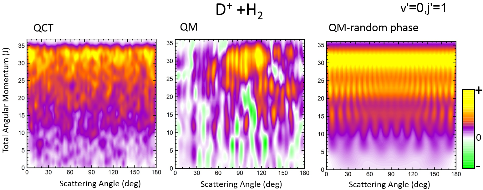
Figure 4: Comparison of the QCT deflection function and the QM analogue deflection function for D⁺ + H₂ reaction at $E_{\rm col}$=0.15 eV. The results are for HD($v^{\prime}$=0, $j^{\prime}$=1).

The results of the CQDF for $\Delta j$=2 are also shown as a dotted lines along with the present $Q_{r}(\theta,J)$. The points corresponding to $\Omega^{\prime}=$0, 1 and 2 are all included. As can be seen, the $\tilde{\Theta}_{\Omega^{\prime}\Omega}(J)$ follows almost exactly the middle line (reproducing the two different slopes) of the present QM-DF and is also in good agrement with the QCT deflection function. More detailed information is shown in Fig. 2, where the $Q_{r}(\theta,J,\Omega^{\prime})$ are plotted separately for each of the three possible $\Omega^{\prime}$ values along with the corresponding CQDF, $\tilde{\Theta}_{\Omega^{\prime}\Omega=0}(J)$. As can be seen, the agreement is excellent and CQDF matches almost exactly the most probable dependence of $\theta$ with $J$ found with the present QM-DF. It should be pointed out, however, that the latter carries information on the intensity of scattering for each $J-\theta$ region, and about the presence of constructive and destructive interferences. Indeed, the information conveyed by the present $Q_{r}(\theta,J,\Omega^{\prime})$ goes well beyond that obtained by the CQDF. As can be seen, most of the intensity of the high-$J$ mechanism corresponds to $\Omega^{\prime}$=2, indicating that the product’s $\bm{j}^{\prime}$ rotational angular momentum lies preferentially along the recoil velocity, whilst that corresponding to low-$J$ is more isotropic with some preference for $\Omega^{\prime}$=1.Aldegunde et al. (2012)

The partial DCS, Eq. (24), and the QM-DF summed over the indicated range of $J$, Eq. (25), are shown in left and right panels of Fig. 3 for $\Delta j$=2 and 4, respectively. The two $J$ intervals have been chosen to comprise partial waves corresponding to the low-$J$ ($J\leq 41$ for $\Delta j$=2 and $J\leq 45$ for $\Delta j$=4) and high-$J$ ($J>41$ for $\Delta j$=2 and $J>45$ for $\Delta j$=4). Therefore, the two magnitudes are broken down in their contributions from the two intervals for comparison purposes. It should be recalled that if the whole range of $J$ is included, both magnitudes become identical, corresponding to the total (converged) DCS. However, whilst the partial DCS only encompasses those coherences only within the chosen interval, the partially summed QM-DF comprises all possible coherences (although their contribution are halved) internal and external to that interval.

The first consideration to be held is the similarity of the respective decompositions of the partial DCSs and the summed QM-DFs $Q_{r}(\theta;\Delta J)$, of the left and right panels. As a second consideration, for $\Delta j=2$, the incoherent sum of $\sigma(\theta;J=0-42)$ and $\sigma(\theta;J>42)$ reproduces fairly well the converged (total) DCS (recall that the partial DCS are not additive), evincing that interferences between the two mechanisms are practically negligible. A similar analysis was performed in Ref. 38 leading to the same conclusion. This is further confirmed by inspection of the $Q_{r}(\theta;\Delta J)$, shown in the right-top panel, which are almost identical to the partial DCSs, except for few differences in the forward region. For the case of $\Delta j=4$ the situation is much the same as that for $\Delta j=2$. The only, main difference between partial DCSs and $Q_{r}(\theta;\Delta J)$ can be observed at forward scattering angles $\theta=$10^∘–30^∘. As can be seen, there is a peak centred on $\theta=12^{\circ}$ in the $Q_{r}(\theta;J<46)$ which is absent in the respective partially summed DCS. This implies that, although without being substantial, there are still some interferences between the two groups of partial waves. Returning to Fig. 1, it is possible to associate this effect with the feature that appears with a ‘hook’ at the top corner of the right-bottom panel of that figure.

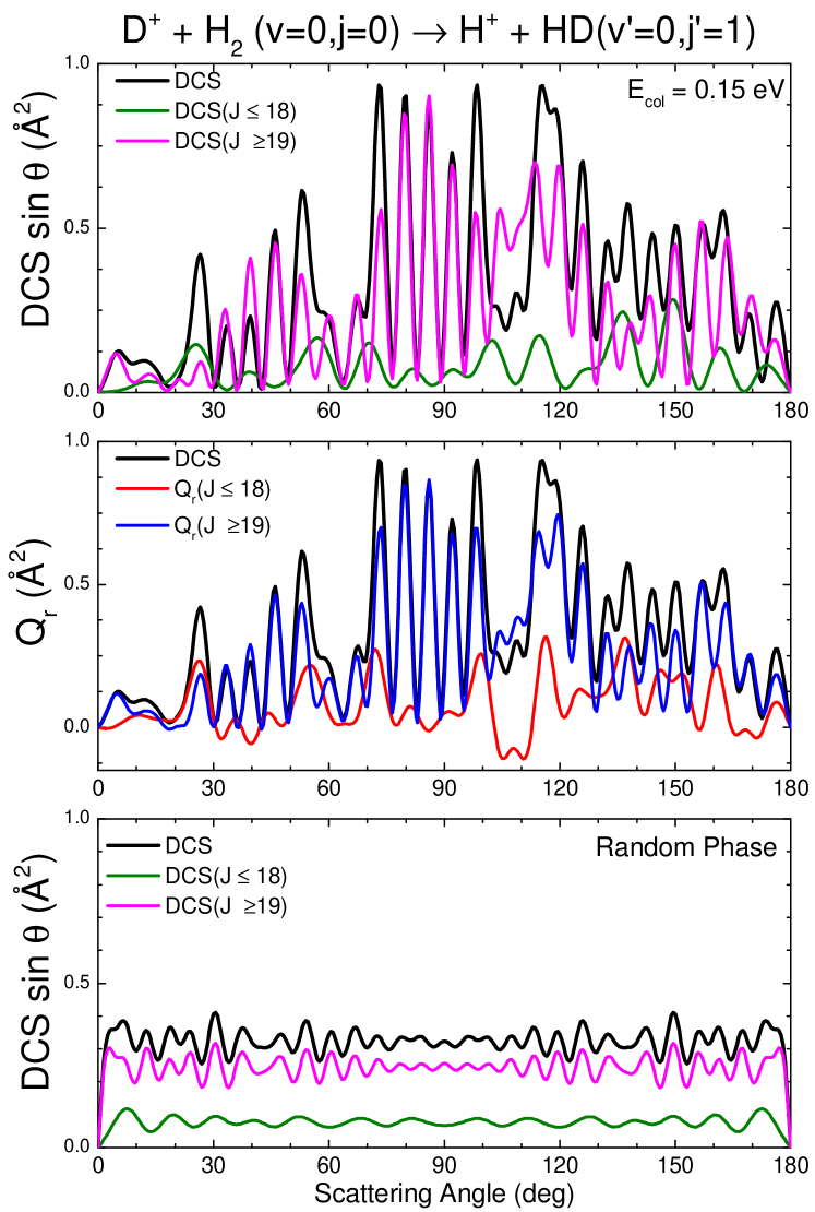
Figure 5: Comparison of the $Q_{r}(J,\theta)$ and the DCS for the D⁺ + H${}_{2}\to$ HD($v^{\prime}$=0,$j^{\prime}$=1) + H⁺ reaction at $E_{\rm col}=$0.15 eV.

It must be pointed out that the above discussion does not imply that for $\Delta j=2$ there are not interferences within one of those groups of partial waves. By inspection of right-bottom panel of Fig. 1, it is obvious that in the forward region and high $J>40$ there are many positive and negative interferences that are the origin of the oscillations observed at $\theta<30^{\circ}$ in Fig. 3.

III.2 Reactions that go throw a long-lived complex, D⁺ + H₂

A contrasting system is the D⁺ + H${}_{2}\to$HD+ H⁺ reaction on its first 1${}^{1}A^{\prime}$ adiabatic PES. As is well known, this PES is barrierless and rather featureless, overwhelmingly dominated by a very deep well of 4 eV from the asymptotes.Aguado et al. (2000); Velilla et al. (2008) Given its importance in astrochemistry, it has been extensively studied both theoretical and experimentally (see, for example, 43; 44; 45; 46; 47; 48; 49; 50; 51; 52; 53 and references therein). It has been long assumed that given the absence of barrier and the presence of a deep well, the H⁺+H₂ reaction could be considered as a prototype of statistical reaction. However, although at low collision energies quantum, quasiclassical and statistical approaches seem to converge yielding results essentially coincident (apart from rapid oscillations), at higher energies, that imply large values of $J$, the centrifugal barrier tends to wash out the potential well potential and QCT calculations indicate that the residence times in the well are too short for the reaction to behave statistically. Jambrina et al. (2009, 2012, 2010, 2010)

We will focus on the results at a sufficiently low energy, $E_{\rm coll}=$ 150 meV and HD($v^{\prime}$=0,$j^{\prime}$=1) formation, where the statistical (ergodic) assumption seems to hold. Indeed, at that energy, the D⁺ + H₂ reaction proceeds through formation of a long-lived complex, the shape of $P(J)$ and the product state distributions follow the trend predicted by statistical methods.Jambrina et al. (2010) Hence, this seems to be a good example to test the reliability of the $Q_{r}(\theta,J)$ in statistical reactions. In Fig. 4 three deflection functions are shown: the classical deflection function, the QM-DF and the quantal one under the assumption of the random phase approximation, which assumes that there is not correlation between different $J$s, so that a deflection function equivalent to the classical one can be calculated. In all three cases, as expected for a statistical reaction, there is no clear correlation between $J$ and $\theta$: all $J$ seems to contribute to every scattering angle. The only remarkable feature in the classical deflection function is the largest probabilities found at high $J$, due to the fact that the $P_{r}(J)$ is flat until it decreases abruptly when reaching $J_{\rm max}$. The $Q_{r}(\theta,J)$, shown in the right panel of Fig. 4, indicates the presence of many destructive (green) and constructive (red/yellow) interferences that will give rise to multiple oscillations in the DCS over the whole range of scattering angles. However, coherences even if they occurred between partial waves with separated $J$ values, are so numerous that their effect is smoothed out to some extent. This is the basic assumption in the random phase approximation,White and Light (1971); Rackham et al. (2001) that allows one to calculate coarse-grained product’s state distributions DCSs and other vector correlations Jambrina et al. (2012) by neglecting the coherences between different total angular momenta, and hence with a formidable saving of computational effort. The right panel of Fig. 3 shows the random phase approximated DF, where all the coherences have been neglected by only keeping the diagonal term, $|f^{J}_{\Omega^{\prime}\Omega}|^{2}$, in Eq. (22). Apart from the discrete character of $J$, the similitude with the QCT deflection function is remarkable. For this reaction we do not show the results obtained using the CQDF as a single valuated function per $J$ cannot account for the complex pattern depicted in Fig.  4. For this reaction, CQDF results in a highly oscillating function due to the superimposed of nearside and farside scattering Hankel and Connor (2015).

The partial and total DCSs, as well as the QM-DF summed over limited ranges of $J$, are shown in the top and middle panel, respectively, of Fig. 5. The $J$ dividing value between low-$J$ and high-$J$ values, has been chosen somewhat arbitrarily as $J_{\max}/2$, since not hint of change of mechanism can be appreciated in neither the QCT nor QM-DF. In the latter case, since no coherences are considered, both magnitudes given by Eqns. (24) and (25) are identical as only the $|f^{J}_{\Omega^{\prime}\Omega}|^{2}$ terms are included. As expected from the QM-DF, the DCSs with the full QM calculation exhibit many oscillations in the whole range of scattering angles, reflecting the numerous interferences that were apparent in Fig. 4. The partial DCSs and their respective $Q(\theta,\Delta J)$ summed in the $[0,18]$ and $[19,35]$ are fairly similar. If we recall that the former are only sensitive to those coherences within the chosen interval whereas the latter includes all of them inside and outside the chosen interval, one can conclude that interferences between separate $J$ values exist but, overall, they almost cancel out.

The partial DCSs, which under the random phase approximation coincides with the $Q_{r}(\theta,\Delta J)$ (summed over $J$) is shown in the bottom panel of Fig. 5, still show some oscillations, nothing surprising considering that they are basically the result of the summation of $[d^{J}_{\Omega\Omega^{\prime}}(\theta)]^{2}$ terms, two for each partial wave. In any case, they correspond, as expected, to the average QM DCSs in which the oscillations have been washed out. The resulting random phase DCSs are strictly symmetric, peaking at forward and backward angles (recall that the represented DCSs have been multiplied by $\sin\theta$). Although at first glance there seems to be a poor approximation of the actual DCSs, but it must be borne in mind that the observed oscillations change rapidly with the collision energy and initial states, hence they would be barely discernible under experimental conditions.

III.3 Direct Reactions: H + D₂

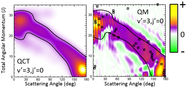
Figure 6: QCT and QM deflection functions for the H + D${}_{2}\to$ HD($v^{\prime}$=3, $j^{\prime}$=0)+D reaction at $E_{\rm col}=$1.73 eV. The contours of the classical deflection functions are copied in the plots representing the QM-DFs to highlight the similarities and differences. The black squares represent the Connor’s $\Theta_{0\,0}(J)$.

The third system we will be concerned with is the H + D₂ reaction, possibly the most widely studied reaction, and indeed the benchmark system in reaction dynamics. Although from many points of view can be considered as the simplest reaction, its dynamics is far richer than it could be expected;Aoiz et al. (2005); Greaves et al. (2008, 2008) indeed, when investigated in detail still renders unexpected results.Dai et al. (2003); Jankunas et al. (2014); Jambrina et al. (2015) Very recently, the angular distributions of state resolved HD formed in collisions between H and D₂ at $E_{\rm col}=1.73$ eV were measured using the photoloc technique.Schafer et al. (1993) For HD($v^{\prime}$=1,low $j^{\prime}$) states the angular distributions in the backward hemisphere were dominated by a series of peaks and dips whose origin was traced to interferences between the two mechanisms described in Refs. 11; 13. For both higher $v^{\prime}$ and/or $j^{\prime}$ rovibrational states, one of the mechanisms disappears and so does the interference pattern in the DCS. In previous works it was shown that the QCT deflection functions was crucial for the right interpretation and assignment of the observed interference pattern.Jambrina et al. (2015, 2016) It can be thus expected that the QM-DF will carry at least the same and presumably even more information about the mechanism. Therefore, the state resolved H + D₂ reaction would be an excellent system to test the quantum analogue to the classical deflection function as we can test its performance under three different scenarios: (i) HD($v^{\prime}$=1,$j^{\prime}$=0) formation, where the interference pattern is conspicuous and dominates the shape of the DCS in the backward hemisphere; (ii) higher $j^{\prime}$, for instance HD($v^{\prime}$=1,$j^{\prime}$=5), where oscillations start to disappear; (iii) higher $v^{\prime}$, v.g., HD($v^{\prime}$=3,$j^{\prime}$=0), where no oscillations were observed in the DCS. In what follows we will show the QM-DF, partial DCS and the QM-DF summed over the appropriate ranges of $J$ for these three different scenarios. All calculations were carried out on the BKMP2 PES.Boothroyd et al. (1996)

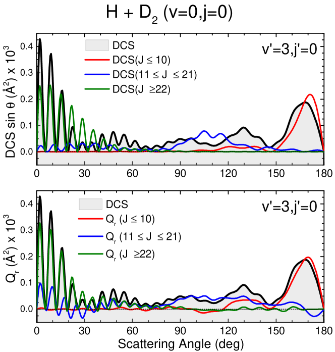
Figure 7: Comparison of the partial DCS (upper panel) and the QM-DF summed over the same $J$ contributions, $Q_{r}(\theta,\Delta J)$ (bottom panel) for the H + D${}_{2}\to$HD($v^{\prime}$=3,$j^{\prime}$=0)+D reaction at $E_{\rm col}=$1.97 eV.

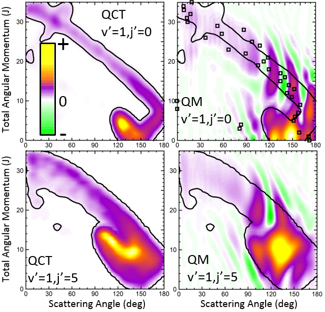
Figure 8: QCT (left) and QM (right) deflection functions for the H + D${}_{2}\to$ HD($v^{\prime}$=0, $j^{\prime}=0,5$)+D reaction at $E_{\rm col}=$1.73 eV. The results for $j^{\prime}$=0 and $j^{\prime}$=5 are shown in the top and bottom panels, respectively. The contours of the classical deflection functions are copied in the plots representing the QM-DFs to highlight the similarities and differences. For the HD($v^{\prime}$=0, $j^{\prime}$=0) formation, Connor’s $\Theta_{0\,0}(J)$ is also represented as black squares.

Let us first turn our attention to those collisions leading to HD($v^{\prime}$=3,$j^{\prime}$=0) whose classical deflection function and QM-DF are depicted in Fig. 6. The QCT deflection function shows the typical profile for a direct reaction mechanism, similar to that observed for the inelastic collisions between Cl and H₂, i.e., a band running diagonally across the $\theta$-$J$ map, with low $J$ giving rise to backward scattering and high $J$ correlating with forward scattering. In this case, the mechanism covers the whole range of scattering angles with one maximum in the forward and another in the backward region. Moreover, there seems to be no other mechanism to compete with it. Not surprisingly, QCT and QM-DFs are very similar, showing the same structure moving from backwards to forwards. However, although the quantum results were somewhat smoothed out for the sake of clarity, we can still observed series of constructive and destructive interferences manifested as stripes, especially in the forward scattering region. In addition, the main band is flanked by two green stripes (destructive interferences) that will give rise to oscillations in the DCS.

Figure 7 depicts the partial DCS and the QM-DF summed over three subsets of partial waves that, according to the deflection functions of Fig. 6, can be associated to backward ($J\in[0,10]$), sideways ($J\in[11,21]$) and forward ($J>22$) scattering. There is a remarkable similitude between the partial DCSs and $Q(\theta,\Delta J)$ for each of the three subsets of $J$ used in the decomposition of these magnitudes, implying that there are essentially no interferences between the partial waves belonging to different subsets. Only at forward scattering angles there are some appreciable interferences between partial waves associated to $J$ values of $J\in[11,21]$ and $J>22$ subsets. There is one more aspect that deserves a comment. The maxima and minima that can be observed in the DCS can be easily inferred from the positive and negative values of the QM-DF. In particular, the minima at 70^∘, 115^∘ and 150^∘ correspond to the negative (green colour) contributions in the QM-DF. These minima (and the precedent or subsequent maxima) cannot be deduced from the classical deflection function.

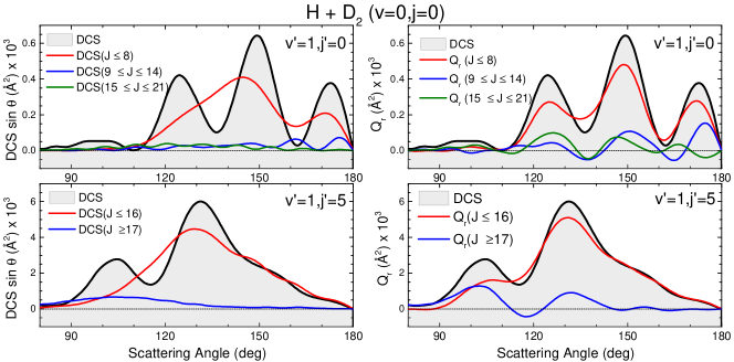
Figure 9: Comparison of the partial DCS (left panels) and $Q_{r}(\theta,\delta J)$ (right panels) for the H + D₂ reaction at $E_{\rm col}=$1.97 eV. Top panels is for scattering giving rise to HD($v^{\prime}$=1,$j^{\prime}$=0), whilst the bottom panel corresponds to $v^{\prime}$=1,$j^{\prime}$=5. Only the backward hemisphere is shown for clarity.

Let us now move to the collisions leading to HD($v^{\prime}$=1,$j^{\prime}$=0). The QCT and QM-DFs are shown in the top panels of Fig. 8. As it was discussed at length in previous work Jambrina et al. (2015), and can be seen by inspection of the QCT deflection function, there are two main, distinct mechanisms that are likely to interact with each other giving rise to the interference pattern observed experimentally. One of them corresponds to the main band with a negative slope, similar to that we have found for $v^{\prime}$=3; the other mechanism, confined in a reduced region of the $J$-$\theta$ map, between 110^∘-160^∘ and low $J$ values, accounts for most of the reactivity. Between them, as a sort of bridge, there is still a third mechanism with a positive slope that comprises low values of $J$ and $\theta>160^{\circ}$. Using the QCT deflection function it easy to predict that interferences will take place,Jambrina et al. (2015) since different paths are leading to the same scattering angles. However, the classical deflection function cannot predict the interference pattern: how many oscillations and what would be their positions. In previous examples, we have shown that the QM-DFs were akin to their QCT counterparts. Admittedly, we could gain some additional information from the formers, but the gist of the processes could be captured by the classical deflection functions. In this example, however, we will see that the quantum $Q_{r}(\theta,J)$ provides an additional and most valuable information.

The first observation is that the QM-DF shown in the top-right panel of Fig. 8 is rather different to its classical counterpart. Only with the help of the superimposed countour of the classical $\sigma_{r}(\theta,J)$ and leaving aside the destructive coherences, we could see that they share the main gross features. Even then, the QM-DF is broader and the region corresponding to the diagonal band almost merges with the mechanism confined between 110^∘-160^∘ and $J<10$. But the main source of discrepancy lies on the presence of negative, destructive (green colour) and positive, constructive (red colour) interferences that do not flank the main band – as in the case of HD($v^{\prime}$=3,$j^{\prime}$=0) scattering– but they are transversal to it, cutting the diagonal band in several slices. Since $Q_{r}(\theta,J)$ are additive, it is easy to realize that each of the slices corresponds to the various peaks in the DCS, whilst the vertical green stripes corresponds to minima in the DCS. Therefore, just looking at the QM-DF we could discern: (i) that there will be three peaks in the backward hemisphere, (ii) which will be their positions, as well as those of the respective minima, and (iii) the partial waves that contribute to each of the peaks.

Not surprisingly, the partial DCS and the QM-DFs summed over range of $J$ values, $Q_{r}(\theta,\Delta J)$, calculated for subsets of partial waves and shown in Fig. 9 do not look alike. The DCS($J\leq 8)$ can be associated to the confined mechanism and, although it carries most of the reactivity, it shows a broad, blunt shape with no hint of the three finger-like peaks present in the total DCS in the 100^∘-180^∘ range. Clearly, the sole consideration of coherences within the $J\in[0,8]$ interval, which are the only ones in the partial DCS, is unable to predict the shape of the DCS. In stark contrast, the $Q_{r}(\theta,0\leq J\leq 8)$, that accounts for all the coherences in and outside the $J\in[0,8]$ range, looks similar to the overall DCS. The partial DCSs calculated for $J>8$ ($J\in[9,14]$ and $J\in[15,21]$) are very small throughout the whole range of scattering angles, whereas their respective $Q_{r}(\theta,\Delta J)$ are not that small. On top of that, at some angles they are negative, a consequence of the negative contour shown in Fig. 8.

The third scenario corresponds to collisions leading to HD($v^{\prime}$=1,$j^{\prime}$=5) whose QCT and QM-DFs are portrayed in the bottom panels of Fig. 8. As can be seen, the structure that was isolated for HD($v^{\prime}$=1,$j^{\prime}$=0) has almost merged into the diagonal band and is considerably less confined. In addition, QCT and QM-DFs look now more alike. Yet the the main band is cut by the signature of a destructive interference (the green slice at $\theta\sim 115^{\circ}$) that can be expected to give rise to a minimum in the backward DCS.

The comparison of the partial DCS and the $Q_{r}(\theta,\Delta J)$ confirm these findings and clarifies the role of interferences. The choice of $J$=16 for the decomposition seems to be a sensible choice at the light of the deflection functions shown in Fig. 8. In contrast to the results for HD($v^{\prime}$=1,$j^{\prime}$=0), the DCS($J\leq 16$) is similar to $Q_{r}(\theta,J\leq 16)$, although the later is somewhat more structured. However, the $Q_{r}(\theta,J\geq 17)$ displays some oscillations and a negative contribution at $\approx 115^{\circ}$ (as expected from the green slice commented on above) that reveals coherences with the low subset of partial waves. The effect of these partial waves is to sharpen the shape of the DCS, defining more clearly the two maxima and the intermediate minimum.

Finally, it is worthwhile to compare the results obtained using the formalism devised in this work with the CQDF. In Figs. 6 and 8, superimposed to the $Q_{r}(\theta,J)$, the respective CQDF for $v^{\prime}$=3 $j^{\prime}$=0 and $v^{\prime}$=1 $j^{\prime}$=0 are represented as open squares. In both cases the agreement is fairly good, covering the regions occupied by the present QM-DF. In particular, the oscillations observed in extreme forward for $v^{\prime}$=3, that could be predicted by the $Q_{r}(\theta,J)$, can be also foreseen using CQDFs (different $J$s leading to the same $\theta$). In fact, using CQDF it can be concluded that they are caused by interferences between nearside and farside reactive flux. Shan and Connor (2012) For the $v^{\prime}$=1 case, however, the sole analysis of the CQDF barely accounts for the confined, predominant mechanism. It must be pointed out that even if we could observe the various mechanisms in the CQDFs, it would have not been possible to predict neither the number of peaks and dips or their position since, for its construction, it only provides one single value of the deflection angle per partial wave.

IV Conclusions

The joint dependence of scattering intensity on the angular momentum and scattering angle, represented by the classical deflection function, has proved to be extremely useful to unravel the mechanism of a colliding system. Indeed, from its inspection one can disentangle reaction mechanisms as well as allows us to predict the presence of interferences. However, the classical deflection function is an ill defined concept on pure quantum mechanical grounds as the differential cross section depends on the coherences between the different values of $J$ caused by the cross terms in the expansion of partial waves. In this work we propose a conceptually simple quantum analogue to the classical deflection function that does account for the coherences and whose interpretation is rather intuitive. Moreover, as it has been defined, the quantum analogue to the classical deflection function (QM-DF) not only relates scattering angles with angular momenta but also accounts for the scattering intensity. As such, summing over the whole set of angular momenta for convergence yields the DCS, and integrating over scattering gives the reactive (or inelastic) partial cross section, similarly to the classical deflection function.

Throughout this article we have applied the proposed QM-DF to several case studies comprising inelastic collisions of Cl+H₂, the barrierless (and presumably statistical) D⁺+H₂ reaction, and the direct H+D₂ reaction for different final states. Our results show that classical and quantum deflection functions are essentially coincident whenever quantum interferences are not preeminent, although the latter are capable of adding valuables details. When quantum phenomena are present, the quantum deflection function arises as a powerful tool and makes possible to observe the interference pattern at first sight, allowing us to disentangle the partial waves that contribute to constructive and destructive interferences. It also provides information on the number and position of the peaks in the DCS, something that cannot be extracted from the classical deflection function. The methodology devised here is completely general, and can be used to obtain deflection functions for polyatomic systems. Moreover, it must be stressed that due to its quantum mechanical nature, it could be used to analyse reaction mechanisms that do not have a classical analogue or under conditions where the classical deflection cannot be calculated, such as at energies below the barrier or whenever either resonances or Fraunhofer diffraction are observed.

V Acknowledgment

The authors acknowledge funding by the Spanish Ministry of Science and Innovation (grant MINECO/FEDER-CTQ2015-65033-P). PGJ acknowledges the Spanish Ministry of Economy and Competitiveness for the Juan de la Cierva fellowship (IJCI-2014-20615).

References

- Levine (2005) R. D. Levine, Molecular Reaction Dynamics, Cambridge University Press, Cambridge, 2005.
- by M. Brouard and Vallance (2010) E. by M. Brouard and C. Vallance, Tutorials in Molecular Reaction Dynamics, RSC Publishing, 2010.
- Eppink and Parker (1997) A. T. J. B. Eppink and D. H. Parker, Rev. Sci. Instrum., 1997, 68, 3477–3484.
- Gijsbertsen et al. (2005) A. Gijsbertsen, H. Linnartz, G. Rus, A. E. Wiskerke and S. Stolte, J. Chem. Phys., 2005, 123, 224305.
- Lin et al. (2003) J. J. Lin, J. Zhou, W. Shiu and K. Liu, Rev. Sci. Instrum., 2003, 74, 2495–2500.
- Ashfold et al. (2006) M. N. R. Ashfold, N. H. Nahler, A. J. Orr-Ewing, O. P. J. Vieuxmaire, R. L. Toomes, T. N. Kitsopoulos, I. A. Garcia, D. A. Chestakov, S.-M. Wu and D. H. Parker, Phys. Chem. Chem. Phys., 2006, 8, 26–53.
- Schafer et al. (1993) N. E. Schafer, A. J. Orr-Ewing, W. R. Simpson, H. Xu and R. N. Zare, Chem. Phys. Lett., 1993, 212, 155.
- Ford and Wheeler (1959) K. W. Ford and J. A. Wheeler, Ann. Phys. (N. Y.), 1959, 7, 259–286.
- Berstein (1966) R. B. Berstein, Advances in Chemical Physics, 1966, 10, 75–134.
- Greaves et al. (2008) S. J. Greaves, D. Murdock and E. Wrede, J. Chem. Phys., 2008, 128, 164307.
- Greaves et al. (2008) S. J. Greaves, D. Murdock, E. Wrede and S. C. Althorpe, J. Chem. Phys., 2008, 128, 164306.
- Feynman et al. (1970) R. P. Feynman, R. B. Leighton and M. Sands, The Feynman Lectures on Physics, Addison Wesley Longman, 1970.
- Jambrina et al. (2015) P. G. Jambrina, D. Herraez-Aguilar, F. J. Aoiz, M. Sneha, J. Jankunas and R. N. Zare, Nat. Chem., 2015, 7, 661–667.
- Jambrina et al. (2016) P. G. Jambrina, J. Aldegunde, F. J. Aoiz, M. Sneha and R. N. Zare, Chem. Sci., 2016, 7, 642–649.
- Sneha et al. (2016) M. Sneha, H. Gao, R. N. Zare, P. G. Jambrina, M. Menendez and F. J. Aoiz, J. Chem. Phys., 2016, 145, 024308.
- Connor (2004) J. N. L. Connor, Phys. Chem. Chem. Phys., 2004, 6, 377–390.
- Shan and Connor (2011) X. Shan and J. N. L. Connor, Phys. Chem. Chem. Phys., 2011, 13, 8392–8406.
- Xiahou and Connor (2009) C. Xiahou and J. N. L. Connor, J. Phys. Chem. A, 2009, 113, 15298–15306.
- Skouteris et al. (2000) D. Skouteris, J. F. Castillo and D. E. Manolopoulos, Comp. Phys. Comm., 2000, 133, 128–135.
- Aoiz et al. (1998) F. J. Aoiz, L. Ba ares and V. J. Herrero, J. Chem. Soc. Faraday. Trans., 1998, 94, 2483–2500.
- Aoiz et al. (1992) F. J. Aoiz, V. J. Herrero and V. S. Rabanos, J. Chem. Phys., 1992, 97, 7423–7436.
- Aoiz et al. (2005) F. J. Aoiz, V. Sáez-Rábanos, B. Martinez-Haya and T. González-Lezana, J. Chem. Phys., 2005, 123, 094101.
- Bonnet and Rayez (1997) L. Bonnet and J. C. Rayez, Chem. Phys. Lett., 1997, 277, 183–190.
- Bañares et al. (2003) L. Bañares, F. Aoiz, P. Honvault, B. Bussery-Honvault and J.-M. Launay, J. Chem. Phys., 2003, 118, 565.
- Bonnet and Rayez (2004) L. Bonnet and J. C. Rayez, Chem. Phys. Lett., 2004, 397, 106–109.
- Aoiz et al. (1992) F. J. Aoiz, V. Herrero and V. S ez-R banos, J. Chem. Phys., 1992, 97, 7423.
- Panda et al. (2012) A. N. Panda, D. Herraez-Aguilar, P. G. Jambrina, J. Aldegunde, S. C. Althorpe and F. J. Aoiz, Phys. Chem. Chem. Phys., 2012, 14, 13067–13075.
- Rackham et al. (2003) E. J. Rackham, T. Gonzalez-Lezana and D. E. Manolopoulos, J. Chem. Phys., 2003, 119, 12895–12907.
- Rackham et al. (2001) E. J. Rackham, F. Huarte-Larranaga and D. E. Manolopoulos, Chem. Phys. Lett., 2001, 343, 356–364.
- Child (1996) M. S. Child, Molecular Collision Theory, Dover publications,, Mineola, N.Y. 11501, 1996.
- Connor (1979) J. N. L. Connor, in Semiclassical methods in Molecular Scattering and Spectroscopy, ed. M. S. Child, Reidel Publishing Company, Dordrecht (Holland), 1979, ch. Semiclassical theory of elastic scattering, p. 45.
- Althorpe and Clary (2003) S. C. Althorpe and D. C. Clary, Ann. Rev. Phys. Chem., 2003, 54, 493–529.
- Alagia et al. (1996) M. Alagia, N. Balucani, L. Cartechini, P. Casavecchia, E. H. van Kleef, G. G. Volpi, F. J. Aoiz, L. Ba ares, D. W. Schwenke, T. C. Allison, S. L. Mielke and D. G. Truhlar, Science, 1996, 273, 1519–1522.
- Casavecchia (2000) P. Casavecchia, Rep. Progr. Phys., 2000, 63, 355–414.
- Wang et al. (2008) X. G. Wang, W. R. Dong, C. L. Xiao, L. Che, Z. F. Ren, D. X. Dai, X. Y. Wang, P. Casavecchia, X. M. Yang, B. Jiang, D. Q. Xie, Z. G. Sun, S. Y. Lee, D. H. Zhang, H. J. Werner and M. H. Alexander, Science, 2008, 322, 573–576.
- Balucani et al. (2003) N. Balucani, D. Skouteris, L. Cartechini, G. Capozza, E. Segoloni, P. Casavecchia, M. H. Alexander, G. Capecchi and H. J. Werner, Phys. Rev. Lett., 2003, 91, 013201.
- Gonzalez-Sanchez et al. (2011) L. Gonzalez-Sanchez, J. Aldegunde, P. G. Jambrina and F. J. Aoiz, J. Chem. Phys., 2011, 135, 064301.
- Aldegunde et al. (2012) J. Aldegunde, F. J. Aoiz, L. Gonzalez-Sanchez, P. G. Jambrina, M. P. de Miranda and V. Saez-Rabanos, Phys. Chem. Chem. Phys., 2012, 14, 2911–2920.
- Bian and Werner (2000) W. S. Bian and H. J. Werner, J. Chem. Phys., 2000, 112, 220–229.
- Greaves et al. (2008) S. J. Greaves, E. Wrede, N. T. Goldberg, J. Zhang, D. J. Miller and R. N. Zare, Nature, 2008, 454, 88.
- Aguado et al. (2000) A. Aguado, O. Roncero, C. Tablero, C. Sanz and M. Paniagua, J. Chem. Phys., 2000, 112, 1240–1254.
- Velilla et al. (2008) L. Velilla, B. Lepetit, A. Aguado, J. A. Beswick and M. Paniagua, Journal of Chemical Physics, 2008, 129, year.
- Gerlich (1993) D. Gerlich, J. Chem. Soc.Far. Trans., 1993, 89, 2199–2208.
- Gerlich (1995) D. Gerlich, Physica Scripta, 1995, T59, 256–263.
- Gerlich and Horning (1992) D. Gerlich and S. Horning, Chem. Rev., 1992, 92, 1509–1539.
- Gerlich and Schlemmer (2002) D. Gerlich and S. Schlemmer, Planet. Space Sci, 2002, 50, 1287–1297.
- Gonzalez-Lezana and Honvault (2017) T. Gonzalez-Lezana and P. Honvault, Mon. Not. R. Astron. Soc., 2017, 467, 1294–1299.
- Jambrina et al. (2009) P. G. Jambrina, F. J. Aoiz, C. J. Eyles, V. J. Herrero and V. Saez-Rabanos, J. Chem. Phys., 2009, 130, 184303.
- Jambrina et al. (2012) P. G. Jambrina, J. M. Alvari o, D. Gerlich, M. Hankel, V. J. Herrero, V. Saez-Rabanos and F. J. Aoiz, Phys. Chem. Chem. Phys., 2012, 14, 3346–3359.
- Jambrina et al. (2010) P. G. Jambrina, F. J. Aoiz, N. Bulut, S. C. Smith, G. G. Balint-Kurti and M. Hankel, Phys. Chem. Chem. Phys., 2010, 12, 1102–1115.
- Jambrina et al. (2010) P. G. Jambrina, J. M. Alvari o, F. J. Aoiz, V. J. Herrero and V. Saez-Rabanos, Phys. Chem. Chem. Phys., 2010, 12, 12591–12603.
- Zanchet et al. (2009) Z. Zanchet, O. Roncero, T. Gonzalez-Lezana, A. Rodriguez-Lopez, A. Aguado, C. Sanz-Sanz and S. Gomez-Carrasco, J. Phys. Chem. A, 2009, 113, 14488.
- Lu et al. (2005) R. F. Lu, T. S. Chu and K. L. Han, J. Phys. Chem. A, 2005, 109, 6683.
- White and Light (1971) R. A. White and J. C. Light, J. Chem. Phys., 1971, 55, 379.
- Jambrina et al. (2012) P. G. Jambrina, J. Aldegunde, M. P. de Miranda, V. Saez-Rabanos and F. J. Aoiz, Phys. Chem. Chem. Phys., 2012, 14, 9977–9987.
- Hankel and Connor (2015) M. Hankel and J. N. L. Connor, AIP Adv., 2015, 5, 077160.
- Aoiz et al. (2005) F. J. Aoiz, L. Ba ares and V. J. Herrero, Int. Rev. Phys. Chem., 2005, 24, 119–190.
- Dai et al. (2003) D. X. Dai, C. C. Wang, S. A. Harich, X. Y. Wang, X. M. Yang, S. D. Chao and R. T. Skodje, Science, 2003, 300, 1730–1734.
- Jankunas et al. (2014) J. Jankunas, M. Sneha, R. N. Zare, F. Bouakline, S. C. Althorpe, D. Herraez-Aguilar and F. J. Aoiz, Proc. Natl. Acad. Sci. USA, 2014, 111, 15–20.
- Boothroyd et al. (1996) A. I. Boothroyd, W. J. Keogh, P. G. Martin and M. R. Peterson, J. Chem. Phys., 1996, 104, 7139–7152.
- Shan and Connor (2012) X. Shan and J. N. L. Connor, J. Chem. Phys., 2012, 136, 044315.