A saturation property for the spectral-Galerkin approximation of a Dirichlet problem in a square

Abstract

Both practice and analysis of adaptive $p$-FEMs and $hp$-FEMs raise the question what increment in the current polynomial degree $p$ guarantees a $p$-independent reduction of the Galerkin error. We answer this question for the $p$-FEM in the simplified context of homogeneous Dirichlet problems for the Poisson equation in the two dimensional unit square with polynomial data of degree $p$. We show that an increment proportional to $p$ yields a $p$-robust error reduction and provide computational evidence that a constant increment does not.

1 Motivation and statement of the result

High order finite element methods (FEMs) exhibit exponential convergence for elliptic problems with piecewise analytic data, and thus have become the methods of choice in computational science and engineering for such problems. The seminal work of Babuška and collaborators [1, 15, 16] has established the mathematical foundations for the a priori design of meshes and distribution of polynomial degrees, and proved exponential convergence for corner and edge singularities. In contrast, adaptive $hp$-FEMs hinge on a posteriori error estimators, which help determine whether it is more convenient to locally refine the mesh or increase the polynomial degree to improve the resolution. Although exponential convergence is observe experimentally, it has never been proved rigorously with the exception of [9].

Our adaptive $hp$-FEM of [9] hinges on a coarsening module due to Binev [6], which in turn guarantees instance optimality and thus exponential convergence. As any other adaptive $hp$-FEM, ours also has a module to reduce the PDE error by a fixed fraction for piecewise polynomial data thereby avoiding data oscillation. Such module in [9] relies on the a posteriori error estimator of Melenk and Wohlmuth [17] for dimension $d=2$ and does not possess optimal complexity. In [10] we turn to the equilibrated flux residual estimator of Braess, Pillwein and Schöberl [7], and Ern and Vorahlík [13, 14], and show that the issue of optimal complexity reduces to studying three model problems with polynomial data in the reference triangle for $d=2$. We present overwhelming computational evidence in [10] supporting the fact that to reduce the Galerkin error by a fixed factor, the polynomial degree $p$ must be increased by an amount proportional to $p$.

In this paper we take over this question again in a further simplified setting and give a rigorous answer. We consider the Poisson equation

$$-\Delta u=f\quad\textrm{in }\Omega,\qquad u=0\quad\textrm{on }\partial\Omega,$$ (1.1)

over the unit square $\Omega=(-1,1)^{2}$ of $\mathbb{R}^{2}$ with polynomial $f$ of degree $p$.

Let us first introduce some notation. Let $I=(-1,1)$ be the reference element so that $\Omega=I^{2}$. For $p\geq 0$, let ${\mathbb{P}}_{p}(\Omega)$ denote the space of polynomials of total degree $\leq p$ restricted to $\Omega$, and let $\mathcal{V}_{p}:={\mathbb{P}}_{p}(\Omega)\cap H^{1}_{0}(\Omega)$. Since the latter space reduces to $\{0\}$ for $p<4$, we will consider it only for $p\geq 4$. We equip $H^{1}_{0}(\Omega)$ with the energy inner product $(\cdot,\cdot)_{H^{1}_{0}(\Omega)}:=(\nabla\cdot,\nabla\cdot)_{L^{2}(\Omega)^{2}}$ and resulting norm $\|\cdot\|_{H^{1}_{0}(\Omega)}$. Analogous definitions apply to $H^{1}_{0}(I)$.

Given any $f\in{\mathbb{P}}_{p}(\Omega)$, let $u=u(f)\in H^{1}_{0}(\Omega)$ be the variational solution of (1.1), i.e.,

$$(u,v)_{H^{1}_{0}(\Omega)}=(f,v)_{L^{2}(\Omega)}\qquad\forall v\in H^{1}_{0}(\Omega).$$ (1.2)

For any $q\geq 4$, let $u_{q}=u_{q}(f)\in\mathcal{V}_{q}$ be the corresponding Galerkin projection of $u$ onto $\mathcal{V}_{q}$, i.e.,

$$(u_{q},v_{q})_{H^{1}_{0}(\Omega)}=(f,v_{q})_{L^{2}(\Omega)}\qquad\forall v\in\mathcal{V}_{q}.$$ (1.3)

We are interested in finding sufficient conditions on $q=q(p)>p$ so that

$$\|u-u_{q}\|_{H^{1}_{0}(\Omega)}\leq\alpha\|u-u_{p}\|_{H^{1}_{0}(\Omega)}$$ (1.4)

for $0<\alpha<1$ independent of $p$. If (1.4) holds, we say that the error reduction is $p$-robust. In view of Phytagoras equality

$$\|u-u_{p}\|_{H^{1}_{0}(\Omega)}^{2}=\|u-u_{q}\|_{H^{1}_{0}(\Omega)}^{2}+\|u_{q}-u_{p}\|_{H^{1}_{0}(\Omega)}^{2},$$ (1.5)

which is a consequence of Galerkin orthogonality $u_{q}-u_{p}\perp u-u_{q}$ in $H^{1}_{0}(\Omega)$, we see that (1.4) is equivalent to the following saturation property

$$\sqrt{1-\alpha^{2}}\,\|u-u_{p}\|_{H^{1}_{0}(\Omega)}\leq\|u_{q}-u_{p}\|_{H^{1}_{0}(\Omega)}.$$ (1.6)

We next observe that (1.6) is equivalent to the simpler saturation property

$$\sqrt{1-\alpha^{2}}\,\|u\|_{H^{1}_{0}(\Omega)}\leq\|u_{q}\|_{H^{1}_{0}(\Omega)}.$$ (1.7)

To see this just define $v:=u-u_{p}\in H^{1}_{0}(\Omega)$, which is the solution of (1.1) with polynomial forcing $f-\Delta u_{p}\in{\color[rgb]{0,0,0}{\mathbb{P}_{p}(\Omega)}}$ and Galerkin solutions $v_{p}=0$ and $v_{q}=u_{q}-u_{p}$. We aim at establishing the following rigorous result.

Theorem 1.1 (saturation property).

There exists a constant $C>0$ such that for all $\lambda>1$, any mapping $p\mapsto q=q(p)$ satisfying $q(p)>\max(\lambda p,p+4)$ yields

$$\|u\|_{H^{1}_{0}(\Omega)}\leq C\frac{\lambda}{\lambda-1}\,\|u_{q}\|_{H^{1}_{0}(\Omega)}\qquad\textrm{for all }\,p\geq 0\text{ and }f\in{\mathbb{P}}_{p}(\Omega).$$ (1.8)

Since most $hp$-FEMs in the literature perform $p$-enrichment upon adding a constant increment to $p$, typically $1$ or $2$, one may wonder whether the preceding sufficient condition on $q$ is also necessary. We now investigate this question computationally upon defining

$$C_{p,q,r}:=\max_{f\in{\color[rgb]{0,0,0}{\mathbb{P}_{p}(\Omega)}}}\frac{\|u_{r}\|_{H^{1}_{0}(\Omega)}}{\|u_{q}\|_{H^{1}_{0}(\Omega)}}$$

where $r\gg q$ is chosen computationally so that $u_{r}$ is sufficiently close to $u$ in $H^{1}_{0}(\Omega)$; note that this is not a hidden saturation assumption because the value of $r$ is not predetermined but found once the number $C_{p,q,r}$ stabilizes. This calculation reduces to an eigenvalue problem, already used in [10], and leads to Figure 1 for $q=p+k$ with $k=2,4,6,10$:

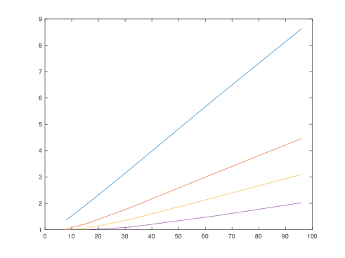
Figure 1: Constants $C_{p,q,r}$ vs $q=p+k$: blue $k=2$, orange $k=4$, yellow $k=6$, violet $k=10$. The dependence is clearly linear rather than constant but the growth is moderate.

We thus realize that $C_{p,q,r}$ exhibits a modest but linear growth on $q=p+k$ for $k$ constant, which confirms that this choice is not $p$-robust. For moderate values of $p$ this might still be acceptable computationally, but it could compromise computational complexity for extreme values of $p$ as in spectral algorithms [8].

Even though the saturation property is quite delicate, it has been often used in a posteriori error analysis of low order AFEMs until now. It originates in the work of Bank and Weiser [2], and Bornemann, Erdmann and Kornhuber [3]; see Nochetto [18] for related work. Dörfler and Nochetto [12] proved the saturation property for $p=1,q=2$ and $d=2$ provided data oscillation is small relative to $\|u-u_{p}\|_{H^{1}_{0}(\Omega)}$ but showed counterexamples for piecewise constant forcing $f$.

We stress that (1.8) is not asymptotic: it is valid for any $p\geq 0$ and any $f\in\mathbb{P}_{p}(\Omega)$. Since $u_{q}\to u$ in $H^{1}_{0}(\Omega)$ as $q\to\infty$ it is obvious that $C_{p,q,\infty}\to 1$ as $q\to\infty$. It is for this reason that Theorem 1.1 has some intrinsic value in the theory of FEMs and might have implications beyond a posteriori error analysis.

The proof of Theorem 1.1 proceeds as follows. We perform a multilevel decomposition of $\mathcal{V}_{q}$

$$\mathcal{V}_{q}=\bigoplus_{j=1}^{q}\mathcal{W}_{j},$$ (1.9)

where $\mathcal{W}_{j}$ are polynomial subspaces of total degree $j$. Since this decomposition is quasi-orthogonal in the sense that

$$\mathcal{W}_{j}\perp\mathcal{W}_{\ell}\quad\textrm{for all }\ell\neq j-2,j,j+2,$$

we need to account for interactions between neighboring spaces $\mathcal{W}_{j}$. We study the angle between subspaces $\mathcal{W}_{j}$ and show it is larger than $\pi/3$; this is the content of Proposition 2.2. This in turn allows us to find the precise decay of high frequency modes of $u_{q}$, which leads to (1.7).

The paper is organized as follows. In section 2 we introduce the multilevel decomposition (1.9) and discuss a few properties including Proposition 2.2. In section 3 we analyze the decay of high order components of $u_{q}$, whereas in section 5 we prove Theorem 1.1. We conclude in section 6 with the proof of the rather technical Proposition 2.2.

2 Multi-level decompositions of polynomial spaces

Hereafter, we recall the definition of classical polynomial bases in $L^{2}(\Omega)$ and in $H^{1}_{0}(\Omega)$, obtained by tensorization from corresponding bases in $L^{2}(I)$ and in $H^{1}_{0}(I)$, where $I=(-1,1)$ is the reference interval. The elements of theses bases enjoy certain orthogonality properties, by which a multi-level, quasi-orthogonal decomposition of $H^{1}_{0}(\Omega)$ is obtained. This will be useful in deriving the main result of this paper.

On the interval $I$, we consider the orthonormal Legendre basis in $L^{2}(I)$

$$\vartheta_{k}(x)=\sqrt{k+\tfrac{1}{2}}\,L_{k}(x),\qquad k\geq 0,$$ (2.1)

(where $L_{k}$ stands for the $k$-th Legendre orthogonal polynomial in $I$, which satisfies ${\rm deg}\,L_{k}=k$ and $L_{k}(1)=1$), as well as the orthonormal Babuška-Shen (BS) basis in $H^{1}_{0}(I)$:

$$\begin{split}\varphi_{k}({x})&=\sqrt{k-\tfrac{1}{2}}\int_{{x}}^{1}L_{k-1}(s)\,{d}s\\ &=\frac{1}{\sqrt{4k-2}}\big{(}L_{k-2}({x})-L_{k}({x})\big{)},\qquad k\geq 2\;.\end{split}$$ (2.2)

The BS basis enjoys the following orthogonality properties in $L^{2}(I)$ for $m\geq k$:

$$(\varphi_{k},\varphi_{m})_{L^{2}({I})}=\begin{cases}\frac{2}{(2k-3)(2k+1)}&\text{if }m=k\;,\\ -\frac{1}{(2k+1)\sqrt{(2k-1)(2k+3)}}&\text{if }m=k+2\;,\\ 0&\text{otherwise.}\end{cases}$$ (2.3)

On the square $\Omega=I\times I$, the previous bases induce, resp., the tensorized orthonormal Legendre basis in $L^{2}(\Omega)$:

$$\Theta_{k}(x)=\vartheta_{k_{1}}(x_{1})\vartheta_{k_{2}}(x_{2}),\qquad k\in\hat{\cal K},$$ (2.4)

where $k=(k_{1},k_{2})$, $x=(x_{1},x_{2})$ and $\hat{\cal K}=\mathbb{N}^{2}$, and the tensorized Babuška-Shen basis in $H^{1}_{0}(\Omega)$:

$$\Phi_{k}(x)=\varphi_{k_{1}}(x_{1})\varphi_{k_{2}}(x_{2}),\qquad k\in{\cal K}\;,$$ (2.5)

where ${\cal K}=\{k\in\mathbb{N}^{2}\ :\ k_{i}\geq 2\text{ for }i=1,2\}$.

The tensorized BS basis is not orthogonal in $H^{1}_{0}(\Omega)$. Indeed, from the expression

$$(\Phi_{k},\Phi_{m})_{H^{1}_{0}(\Omega)} =(\varphi_{k_{1}},\varphi_{m_{1}})_{H^{1}_{0}({I})}(\varphi_{k_{2}},\varphi_{m_{2}})_{L^{2}({I})}$$

$$+(\varphi_{k_{1}},\varphi_{m_{1}})_{L^{2}({I})}(\varphi_{k_{2}},\varphi_{m_{2}})_{H^{1}_{0}({I})}\;,$$

and (2.3) we immediately obtain

$$(\Phi_{k},\Phi_{m})_{H^{1}_{0}(\Omega)}\not=0\text{ \ iff \ }\begin{cases}k_{1}=m_{1}\text{ and }k_{2}-m_{2}\in\{-2,0,2\},\text{ or }\\ k_{2}=m_{2}\text{ and }k_{1}-m_{1}\in\{-2,0,2\}.\end{cases}$$ (2.6)

As a consequence, denoting by $|k|=|k_{1}|+|k_{2}|$ the $\ell^{1}$-norm in $\mathbb{Z}^{2}$, we have

$$(\Phi_{k},\Phi_{m})_{H^{1}_{0}(\Omega)}=0\qquad\text{if \ }|k|-|m|\not\in\{-2,0,2\}.$$ (2.7)

At last, concerning the interaction between the Legendre basis and the BS one, we have

$$(\Theta_{k},\Phi_{m})_{L^{2}(\Omega)}\not=0\text{ \ iff \ }k_{1}\in\{m_{1}-2,m_{1}\}\text{ and }k_{2}\in\{m_{2}-2,m_{2}\},$$ (2.8)

which implies

$$(\Theta_{k},\Phi_{m})_{L^{2}(\Omega)}=0\qquad\text{if \ }|k-m|>4.$$ (2.9)

Remark 2.1 (orthogonality by parity).

Any function $v\in L^{2}(\Omega)$ can be split uniquely into four components

$$v=\sum_{\alpha\in\{0,1\}^{2}}v^{\alpha},$$ (2.10)

where $v^{\alpha}$ for $\alpha=(\alpha_{1},\alpha_{2})$ is even (odd, resp.) with respect to the variable $x_{i}$ ($i=1,2$) iff $\alpha_{i}=0$ ($\alpha_{i}=1$, resp.). For instance, $v^{(0,1)}$ satisfies $v^{(0,1)}(-x_{1},x_{2})=v^{(0,1)}(x_{1},x_{2})$ and $v^{(0,1)}(x_{1},-x_{2})=-v^{(0,1)}(x_{1},x_{2})$ for all $(x_{1},x_{2})\in\Omega$.

Components with different parity indices are always $L^{2}(\Omega)$-orthogonal, and $H^{1}_{0}(\Omega)$-orthogonal whenever $v\in H^{1}_{0}(\Omega)$. In particular, as a consequence of (2.6) and (2.8), we observe that $(\Phi_{k},\Phi_{m})_{H^{1}_{0}(\Omega)}=0$ and $(\Theta_{k},\Phi_{m})_{L^{2}(\Omega)}=0$ whenever $k$ and $m$ have at least one entry of different parity.

2.1 Detail spaces and their projectors

For $j\geq 4$, let us define the finite dimensional subspace of $H^{1}_{0}(\Omega)$

$$\mathcal{W}_{j}:=\text{span}\{\Phi_{k}\,:|k|=j\}\;.$$ (2.11)

Note that, thanks to (2.6), the functions $\Phi_{k}$ that generate $\mathcal{W}_{j}$ are mutually orthogonal in $H^{1}_{0}(\Omega)$. We immediately have the multi-level decompositions

$$\mathcal{V}_{q}=\bigoplus_{j=4}^{q}\mathcal{W}_{j}\quad\textrm{for all }q\geq 4\qquad\text{and}\qquad H^{1}_{0}(\Omega)=\bigoplus_{j=4}^{\infty}\mathcal{W}_{j}\;.$$ (2.12)

Such decompositions are ‘quasi-orthogonal’, in the sense that by (2.7) we have

$$\mathcal{W}_{j}\perp_{H^{1}_{0}(\Omega)}\mathcal{W}_{\ell}\qquad\text{for all \ }\ell\not=j-2,j,j+2.$$ (2.13)

Furthermore, the ‘angle’ between two non-orthogonal subspaces is uniformly bounded away from 0, as implied by the following technical result, that will be crucial in the sequel. We postpone its proof to section 6.

Proposition 2.2 (angle between $\mathcal{W}_{j-2}$ and $\mathcal{W}_{j}$).

Let $P_{j}:\mathcal{W}_{j-2}\to\mathcal{W}_{j}$ ($j\geq 6$) be the orthogonal projection with respect to the $H^{1}_{0}(\Omega)$-inner product. Then,

$$\|P_{j}\|_{{\cal L}(\mathcal{W}_{j-2},\mathcal{W}_{j})}<\frac{1}{2}.$$

Actually, there exists a constant $c>0$ independent of $j$ such that

$$\|P_{j}\|_{{\cal L}(\mathcal{W}_{j-2},\mathcal{W}_{j})}\leq\frac{1}{2}\left(1-\frac{c}{\,j^{2}}\right)\;.$$

Note that the orthogonal projection $P_{j}^{*}:\mathcal{W}_{j}\to\mathcal{W}_{j-2}$, given by the adjoint of $P_{j}$, satisfies the same estimate.

3 Decay of the higher-order components of the Galerkin solution

Given $f\in{\mathbb{P}}_{p}(\Omega)$, let $u_{q}\in\mathcal{V}_{q}$ be the Galerkin solution defined in (1.3), and let $u_{q}=\sum_{j=4}^{q}U_{j}$, with $U_{j}=U_{j}(q)\in\mathcal{W}_{j}$, be its multilevel decomposition according to (2.12). The purpose of this section is to prove that for any $q$ sufficiently larger than $p$, the $H^{1}_{0}(\Omega)$-norm of $U_{q}$ and $U_{q-1}$ decay at least proportionally to the quantity $(q-p)^{-1}$. The precise result is as follows.

Proposition 3.1 (decay of $U_{j}$).

For any $p\geq 0$ and $q>\hat{p}:=p+4$, one has

$$\|U_{j}\|_{H^{1}_{0}(\Omega)}\leq\frac{6}{q-p}\,\|u_{q}\|_{H^{1}_{0}(\Omega)}\;,\qquad j=q,\,q-1.$$ (3.1)

Proof.

We first observe that the parity splitting (2.10) of the forcing $f$ induces by linearity a corresponding splitting of the Galerkin solution $u_{q}$ as well as of each of its multi-level details $U_{j}$, which is nothing but the parity splitting of $u_{q}$ as well as of $U_{j}$. Therefore, thanks to the orthogonality of the components with different parity (cf. Remark 2.1), it is enough to establish (3.1) for each component separately, and then sum-up the squares of both sides invoking Parseval’s identity.

For the sake of definiteness, we will focus on the components of (even, even) type, the other types being amenable to a similar treatment. Thus, referring to (2.10) for the notation, we consider the component $u_{q}^{(0,0)}$ of $u_{q}$ (which solves (1.3) for the forcing $f^{(0,0)}$), as well as its details $U_{j}^{(0,0)}\in\mathcal{W}_{j}^{(0,0)}:=\text{span}\{\Phi_{k}\,:|k|=j\text{ and }k_{1},k_{2}\text{ are even}\}$. We aim at proving that for $q\geq\hat{p}+1$ and $j\in\{q-1,q\}$

$$\|U_{j}^{(0,0)}\|_{H^{1}_{0}(\Omega)}\leq\frac{6}{q-p}\,\|u_{q}^{(0,0)}\|_{H^{1}_{0}(\Omega)}.$$

However, it is easily seen that $U_{q-1}^{(0,0)}=0$ if $q$ is even, and similarly $U_{q}^{(0,0)}=0$ if $q$ is odd. Hence, we will prove

$$\|U_{q}^{(0,0)}\|_{H^{1}_{0}(\Omega)}\leq\frac{6}{q-p}\,\|u_{q}^{(0,0)}\|_{H^{1}_{0}(\Omega)}$$ (3.2)

under the assumption that $q$ is even, the other situation being similar.

To avoid cumbersome notation, for the rest of the proof we will drop the superscript $\phantom{u}{}^{(0,0)}$ from all entities. So, we will write

$$u_{q}=\sideset{}{{}^{\prime}}{\sum}\limits_{j=4}^{q}U_{j}\qquad\textrm{with }U_{j}\in\mathcal{W}_{j},$$

where here and in the sequel the symbol ${}^{{}^{\prime}}$ indicates that the summation runs over even indices only.

From the Galerkin equations, we have for any even $j\in[4,q]$

$$(u_{q},W_{j})_{H^{1}_{0}(\Omega)}=(f,W_{j})_{L^{2}(\Omega)}\qquad\textrm{for all }W_{j}\in\mathcal{W}_{j}\;.$$ (3.3)

Since $q\geq\hat{p}+1$, exploiting (2.7) and (2.8), (3.3) yields

$$(U_{q},W_{q})_{H^{1}_{0}(\Omega)}+(U_{q-2},W_{q})_{H^{1}_{0}(\Omega)}=0\qquad\textrm{for all }W_{q}\in\mathcal{W}_{q}\;,$$ (3.4)

which can be rewritten equivalently as

$$U_{q}=-T_{q}^{-1}P_{q}U_{q-2}$$ (3.5)

where $T_{q}=I$ and $P_{q}$ is defined in Proposition 2.2.

For any even $j$ satisfying $\hat{p}+2<j\leq q-2$, (3.3) yields

$$(U_{j+2},W_{j})_{H^{1}_{0}(\Omega)}+(U_{j},W_{j})_{H^{1}_{0}(\Omega)}+(U_{j-2},W_{j})_{H^{1}_{0}(\Omega)}=0\qquad$$ (3.6)

for all $W_{j}\in\mathcal{W}_{j}$; this is equivalent to $P_{j+2}^{*}U_{j+2}+U_{j}+P_{j}U_{j-2}=0$. Assuming by induction that $U_{j+2}=-T_{j+2}^{-1}P_{j+2}U_{j}$ with $\|T_{j+2}^{-1}\|\leq 2$ (which is trivially true for $j=q-2$ according to (3.5)), gives

$$(I-P_{j+2}^{*}T_{j+2}^{-1}P_{j+2})U_{j}=-P_{j}U_{j-2}.$$

Using Proposition 2.2, the operator

$$T_{j}:=I-P_{j+2}^{*}T_{j+2}^{-1}P_{j+2}$$ (3.7)

is invertible and satisfies

$$\|T^{-1}_{j}\|\leq\frac{1}{1-\frac{1}{4}\|T^{-1}_{j+2}\|}\;.$$ (3.8)

We conclude that

$$U_{j}=-T_{j}^{-1}P_{j}U_{j-2}.$$ (3.9)

with $\|T^{-1}_{j}\|\leq 2$, which proves the induction argument for all even $j$ satisfying $\hat{p}+2<j\leq q-2$.

Next, we have to bound the norm of $U_{j-2}$ for $j=\hat{p}+4$ when $p$, hence $\hat{p}$, is even, or for $j=\hat{p}+3$ when $p$ is odd. It is therefore convenient to define the even integer

$$r:=\begin{cases}\hat{p}=p+4&\text{if }p\text{ is even},\\ \hat{p}-1=p+3&\text{if }p\text{ is odd},\end{cases}$$

so that in both cases, we have to bound $\|U_{r+2}\|_{H^{1}_{0}(\Omega)}$. To this end, let us introduce

$$\mathcal{V}_{r}^{(0,0)}:=\sideset{}{{}^{\prime}}{\bigoplus}_{j=4}^{r}\mathcal{W}_{j},\qquad\bar{u}_{r}:=\sideset{}{{}^{\prime}}{\sum}\limits_{j=4}^{r}U_{j}\in\mathcal{V}_{r}^{(0,0)};$$

note that $\bar{u}_{r}\neq u_{r}$ because $U_{j}=U_{j}(q)$. Then, in view of (3.3), we deduce

$$(\bar{u}_{r}+\sideset{}{{}^{\prime}}{\sum}_{j=r+2}^{q}U_{j},v_{r})_{H^{1}_{0}(\Omega)}=(f,v_{r})_{L^{2}(\Omega)}\quad\textrm{for all }v_{r}\in\mathcal{V}_{r}^{(0,0)}\;,$$ (3.10)

which, thanks to $\displaystyle{(\sideset{}{{}^{\prime}}{\sum}_{j=r+2}^{q}U_{j},v_{r})_{H^{1}_{0}(\Omega)}}=(P_{r}^{*}U_{r+2},v_{r})_{H^{1}_{0}(\Omega)}$ for all $v_{r}\in\mathcal{V}_{r}^{(0,0)}$, implies that

$$\bar{u}_{r}+P_{r}^{*}U_{r+2}=u_{r}.$$

We observe that (3.6) is also valid for $j=r+2$. Since $(U_{r},W_{r+2})_{H^{1}_{0}(\Omega)}=(\bar{u}_{r},W_{r+2})_{H^{1}_{0}(\Omega)}$ we obtain

$$(U_{r+4},W_{r+2})_{H^{1}_{0}(\Omega)}+(U_{r+2},W_{r+2})_{H^{1}_{0}(\Omega)}+(\bar{u}_{r},W_{r+2})_{H^{1}_{0}(\Omega)}=0$$ (3.11)

and

$$T_{r+2}U_{r+2}=-P_{r+2}\bar{u}_{r}$$

as it happened with (3.9). This implies

$$(T_{r+2}-P_{r+2}P_{r}^{*})U_{r+2}=-P_{r+2}u_{r}$$ (3.12)

which in view of (3.7) yields

$$(I-P_{r+4}^{*}T_{r+4}^{-1}P_{r+4}-P_{r+2}P_{r}^{*})U_{r+2}=-P_{r+2}u_{r}.$$ (3.13)

Since $\|P_{r+4}^{*}T_{r+4}^{-1}P_{r+4}+P_{r+2}P_{r}^{*}\|\leq 2\frac{1}{4}+\frac{1}{4}=\frac{3}{4}$, thanks to Proposition 2.2 and $\|T_{r+4}^{-1}\|\leq 2$, we conclude that

$$\|U_{r+2}\|_{H^{1}_{0}(\Omega)}\leq\frac{1}{1-\frac{3}{4}}\frac{1}{2}\|u_{r}\|_{H^{1}_{0}(\Omega)}=2\|u_{r}\|_{H^{1}_{0}(\Omega)}\leq 2\|u_{q}\|_{H^{1}_{0}(\Omega)},$$

where last inequality follows from the inclusion $\mathcal{V}_{r}^{0,0)}\subset\mathcal{V}_{q}^{(0,0)}$ and the minimization property of the Galerkin solution.

Collecting the above results we arrive at

$$\begin{split}&U_{j}=-T_{j}^{-1}P_{j}U_{j-2}\qquad r+4\leq j\leq q\quad\text{($j$ even)},\\ &\|U_{r+2}\|_{H^{1}_{0}(\Omega)}\leq 2\|u_{q}\|_{H^{1}_{0}(\Omega)}.\end{split}$$ (3.14)

For $q\geq\hat{p}+4$, this implies

$$\|U_{q}\|_{H^{1}_{0}(\Omega)}\leq\sideset{}{{}^{\prime}}{\prod}_{j=r+4}^{q}\|T_{j}^{-1}P_{j}\|\|U_{r+2}\|_{H^{1}_{0}(\Omega)}\leq 2\|u_{q}\|_{H^{1}_{0}(\Omega)}\sideset{}{{}^{\prime}}{\prod}_{j=r+4}^{q}\|T_{j}^{-1}P_{j}\|.$$

In order to bound the product on the right-hand side, let us write $j=q-2m$ with $m=0,1,\dots,s$ and $s:=\frac{1}{2}(q-r)-2$. Then, by Proposition 2.2, we have $\|T_{j}^{-1}P_{j}\|\leq\frac{1}{2}\|T_{j}^{-1}\|=:\alpha_{m}$. Recalling (3.8), it holds

$$\alpha_{m}\leq\frac{\frac{1}{2}}{1-\frac{1}{2}\alpha_{m-1}}=\frac{1}{2-\alpha_{m-1}},\qquad\text{with \ }\alpha_{0}\leq\tfrac{1}{2}\;.$$

By recurrence, it is immediate to check that $\alpha_{m}\leq\frac{m+1}{m+2}$, whence

$$\sideset{}{{}^{\prime}}{\prod}_{j=r+4}^{q}\|T_{j}^{-1}P_{j}\|\leq\prod_{m=0}^{s}\alpha_{m}\leq\prod_{m=0}^{s}\frac{m+1}{m+2}=\frac{1}{s+2}=\frac{2}{q-r}.$$

Since $q\geq p+6$ if $p$ is even and $q\geq p+5$ if $p$ is odd, it is easily checked that

$$\frac{2}{q-r}=\begin{cases}\frac{2}{(q-p)-4}\leq\frac{6}{q-p}&\text{if }p\text{ is even},\\ \frac{2}{(q-p)-3}\leq\frac{5}{q-p}&\text{if }p\text{ is odd}.\end{cases}$$

This gives the desired estimate (3.2). ∎

4 A subspace decomposition in $H^{1}_{0}(\Omega)$

Consider the complementary space of $\mathcal{V}_{q}$ in $H^{1}_{0}(\Omega)$ given by

$$\mathcal{V}_{q}^{c}:=\operatorname{clos}_{H^{1}_{0}(\Omega)}\text{span}\,\{\Phi_{m}\,:\,|m|>q\}.$$ (4.1)

Therefore, $H^{1}_{0}(\Omega)=\mathcal{V}_{q}\oplus\mathcal{V}_{q}^{c}$ and any $v\in H^{1}_{0}(\Omega)$ can be split as

$$v=v_{q}+z_{q},\qquad v_{q}\in\mathcal{V}_{q},\quad z_{q}\in\mathcal{V}_{q}^{c}.$$

The purpose of this section is to apply once more Proposition 2.2 and derive a bound on the norm of $v_{q}$ and $z_{q}$ in terms of the norm of $v$.

We start with the following auxiliary result for any $w=\sum_{j=4}^{q}W_{j}\in\mathcal{V}_{q}.$

Lemma 4.1 (bound of $\|W_{q}\|_{H^{1}_{0}(\Omega)}$).

For any $q\geq 4$ and any $w=\sum_{j=4}^{q}W_{j}\in\mathcal{V}_{q}$, one has

$$\|W_{q}\|_{H^{1}_{0}(\Omega)}\leq\sqrt{2}\|w\|_{H^{1}_{0}(\Omega)}\;.$$

Proof.

As in the previous section, splitting $w$ and $W_{q}$ in their orthogonal components according to the parity of the basis functions, it is enough to establish the result for each component separately. Hereafter, we detail the analysis for the ‘(even, even)’ case, in which case we may assume $q$ even, since otherwise $W_{q}^{(0,0)}=0$ and the result is trivial.

Dropping as above the superscript $\phantom{u}{}^{(0,0)}$ in functions and subspaces, we write $w=W+W_{q}$ with

$$W=\sideset{}{{}^{\prime}}{\sum}\limits_{j=4}^{q-2}W_{j}\in\mathcal{V}_{q-2}.$$

Keeping $W_{q}$ fixed, let us first minimize the norm of $w$, i.e., let us look for the minimizer $\bar{W}\in\mathcal{V}_{q-2}$ of the quantity $\Psi(W):=\|W+W_{q}\|_{H^{1}_{0}(\Omega)}^{2}$. Such a function satisfies

$$(\bar{W},Y)_{H^{1}_{0}(\Omega)}=-(W_{q},Y)_{H^{1}_{0}(\Omega)}\qquad\textrm{for all }Y\in\mathcal{V}_{q-2}$$ (4.2)

and

$$\Psi(\bar{W})=\|W_{q}\|_{H^{1}_{0}(\Omega)}^{2}+(W_{q},\bar{W})_{H^{1}_{0}(\Omega)}\;.$$ (4.3)

Using the orthogonality conditions (2.7), we obtain the sequence of equations

$$(\bar{W}_{4},Y_{4})_{H^{1}_{0}(\Omega)}+(\bar{W}_{6},Y_{4})_{H^{1}_{0}(\Omega)}=0\qquad\textrm{for all }Y_{4}\in\mathcal{W}_{4}\;,$$

and

$$(\bar{W}_{j-2},Y_{j})_{H^{1}_{0}(\Omega)}+(\bar{W}_{j},Y_{j})_{H^{1}_{0}(\Omega)}+(\bar{W}_{j+2},Y_{j})_{H^{1}_{0}(\Omega)}=0\qquad\textrm{for all }Y_{j}\in\mathcal{W}_{j}$$

for any even $j$ such that $4<j<q-2$, and finally

$$(\bar{W}_{q-4},Y_{q-2})_{H^{1}_{0}(\Omega)}+(\bar{W}_{q-2},Y_{q-2})_{H^{1}_{0}(\Omega)}=-(W_{q},Y_{q-2})_{H^{1}_{0}(\Omega)}$$

for all $Y_{q-2}\in\mathcal{W}_{q-2}$. Setting recursively $T_{4}=I$ and $T_{j}=(I-P_{j}T_{j-2}^{-1}P_{j}^{*})$, we derive $\bar{W}_{j}=-T_{j}^{-1}P_{j+2}^{*}\bar{W}_{j+2}$ for $j=4,6,\dots,q-4$, and $\bar{W}_{q-2}=-T_{q-2}^{-1}P_{q}^{*}W_{q}$. Note that, thanks to Proposition 2.2, one can prove as in Sect. 3 that $\|T_{j}^{-1}\|\leq 2$ for all $j$. Since

$$(W_{q},\bar{W})_{H^{1}_{0}(\Omega)} =(W_{q},\bar{W}_{q-2})_{H^{1}_{0}(\Omega)}$$

$$=(P_{q}^{*}W_{q},\bar{W}_{q-2})_{H^{1}_{0}(\Omega)}=-(P_{q}^{*}W_{q},T_{q-2}^{-1}P_{q}^{*}W_{q})_{H^{1}_{0}(\Omega)},$$

using once more Proposition 2.2, we deduce

$$(P_{q}^{*}W_{q},T_{q-2}^{-1}P_{q}^{*}W_{q})_{H^{1}_{0}(\Omega)} \leq\|T_{q-2}^{-1}\|\,\|P_{q}^{*}\|^{2}\|W_{q}\|_{H^{1}_{0}(\Omega)}^{2}$$

$$\leq 2\left(\frac{1}{2}\right)^{2}\|W_{q}\|_{H^{1}_{0}(\Omega)}^{2}=\frac{1}{2}\|W_{q}\|_{H^{1}_{0}(\Omega)}^{2}\;.$$

In view of (4.3) and the preceding estimate, we conclude that

$$\|w\|_{H^{1}_{0}(\Omega)}^{2}=\Psi(W)\geq\Psi(\bar{W})\geq\|W_{q}\|_{H^{1}_{0}(\Omega)}^{2}-\frac{1}{2}\|W_{q}\|_{H^{1}_{0}(\Omega)}^{2}=\frac{1}{2}\|W_{q}\|_{H^{1}_{0}(\Omega)}^{2}$$

for any $w\in\mathcal{V}_{q}^{(0,0)}$, whence the asserted estimate follows. ∎

We now establish the main result of this section.

Proposition 4.2 (control of $\|z_{q}\|_{H^{1}_{0}(\Omega)}$).

There exists a constant $C_{2}>0$ such that for any $q\geq 4$ and any $v=v_{q}+z_{q}\in\mathcal{V}_{q}\oplus\mathcal{V}_{q}^{c}$, one has

$$\|z_{q}\|_{H^{1}_{0}(\Omega)}\leq C_{2}\,q\,\|v\|_{H^{1}_{0}(\Omega)}.$$ (4.4)

Proof.

Using $\|z_{q}\|_{H^{1}_{0}(\Omega)}\leq\|v\|_{H^{1}_{0}(\Omega)}+\|v_{q}\|_{H^{1}_{0}(\Omega)}$, it is enough to prove the existence of a constant $C_{2}^{\prime}>0$ independent of $q$ such that for all $v\in H^{1}_{0}(\Omega)$

$$\|v_{q}\|_{H^{1}_{0}(\Omega)}\leq C_{2}^{\prime}q\|v\|_{H^{1}_{0}(\Omega)}\;.$$ (4.5)

To this end, let us focus as above on the ‘(even, even)’ components of $v$ and $v_{q}$, in which case it is not restrictive to assume $q$ even, and drop the superscript $\phantom{u}{}^{(0,0)}$ in functions and subspaces. Let us fix any even integer $r>q$ and assume first that $v\in\mathcal{V}_{r}$ is written as $v=v_{q}+V$, with

$$V=\sideset{}{{}^{\prime}}{\sum}\limits_{j=q+2}^{r}V_{j}\in\sideset{}{{}^{\prime}}{\bigoplus}\limits_{j=q+2}^{r}\mathcal{W}_{j}.$$

By applying the same technique as above, i.e., minimizing the (squared) norm $\Psi(V):=\|v_{q}+V\|_{H^{1}_{0}(\Omega)}^{2}$, we find that

$$\|v\|_{H^{1}_{0}(\Omega)}^{2}=\Psi(V)\geq\Psi(\bar{V})=\|v_{q}\|_{H^{1}_{0}(\Omega)}^{2}+(v_{q},\bar{V})_{H^{1}_{0}(\Omega)}\;,$$ (4.6)

where the minimizer $\bar{V}=\sideset{}{{}^{\prime}}{\sum}\limits_{j=q+2}^{r}\bar{V}_{j}$ is such that $\bar{V}_{q+2}=-T_{q+2}^{-1}\tilde{P}_{q+2}v_{q}$, for $T_{q+2}$ defined recursively by (3.7) with $T_{r}=I$, and $\tilde{P}_{q+2}:H^{1}_{0}(\Omega)\to\mathcal{W}_{q+2}$ defined as the orthogonal projection in the $H^{1}_{0}(\Omega)$ inner product. Now,

$$(v_{q},\bar{V})_{H^{1}_{0}(\Omega)} =(v_{q},\bar{V}_{q+2})_{H^{1}_{0}(\Omega)}=(\tilde{P}_{q+2}v_{q},\bar{V}_{q+2})_{H^{1}_{0}(\Omega)}$$

$$=-(\tilde{P}_{q+2}v_{q},T_{q+2}^{-1}\tilde{P}_{q+2}v_{q})_{H^{1}_{0}(\Omega)}$$

with

$$\big{|}(\tilde{P}_{q+2}v_{q},T_{q+2}^{-1}\tilde{P}_{q+2}v_{q})_{H^{1}_{0}(\Omega)}\big{|}\leq\|T_{q+2}^{-1}\|\,\|\tilde{P}_{q+2}v_{q}\|_{H^{1}_{0}(\Omega)}^{2}\leq 2\|\tilde{P}_{q+2}v_{q}\|_{H^{1}_{0}(\Omega)}^{2}\;.$$

Writing $v_{q}=\sideset{}{{}^{\prime}}{\sum}\limits_{j=4}^{q}V_{j}$, one has $\tilde{P}_{q+2}v_{q}=\tilde{P}_{q+2}V_{q}=P_{q+2}V_{q}$, whence by Proposition 2.2 with $\varepsilon_{j}=cj^{-2}$ and Lemma 4.1 we get

$$\|\tilde{P}_{q+2}v_{q}\|_{H^{1}_{0}(\Omega)}=\|P_{q+2}V_{q}\|_{H^{1}_{0}(\Omega)} \leq\frac{1}{2}\left(1-\varepsilon_{q+2}\right)\|V_{q}\|_{H^{1}_{0}(\Omega)}$$

$$\leq\frac{1}{\sqrt{2}}\left(1-\varepsilon_{q+2}\right)\|v_{q}\|_{H^{1}_{0}(\Omega)}\;,$$

which gives

$$\big{|}(\tilde{P}_{q+2}v_{q},T_{q+2}^{-1}\tilde{P}_{q+2}v_{q})_{H^{1}_{0}(\Omega)}\big{|}\leq\left(1-\varepsilon_{q+2}\right)^{2}\|v_{q}\|_{H^{1}_{0}(\Omega)}^{2}\;.$$

Then, from (4.6) we obtain

$$\|v\|_{H^{1}_{0}(\Omega)}^{2}\geq\varepsilon_{q+2}(2-\varepsilon_{q+2})\|v_{q}\|_{H^{1}_{0}(\Omega)}^{2}\;,$$

which immediately yields (4.5) for all $v\in\mathcal{V}_{r}=\mathcal{V}_{r}^{(0,0)}$ and all $r>q$.

The same result holds for all other combinations of parity indices; hence, it holds for any $v\in\mathcal{V}_{r}$. Since polynomials vanishing on $\partial\Omega$ form a dense subset of $H^{1}_{0}(\Omega)$, we conclude that (4.5) holds for all $v\in H^{1}_{0}(\Omega)$. ∎

5 Proof of Theorem 1.1

We actually prove the equivalent condition

$$\|u-u_{q}\|_{H^{1}_{0}(\Omega)}\lesssim\|u_{q}\|_{H^{1}_{0}(\Omega)},$$

and for that we write

$$\|u-u_{q}\|_{H^{1}_{0}(\Omega)}=\sup_{v\in H^{1}_{0}(\Omega),\ v\not=0}\frac{(u-u_{q},v)_{H^{1}_{0}(\Omega)}}{\|v\|_{H^{1}_{0}(\Omega)}}.$$

As in the previous section, let us split any $v\in H^{1}_{0}(\Omega)$ as $v=v_{q}+z_{q}\in\mathcal{V}_{q}\oplus\mathcal{V}_{q}^{c}$, where $\mathcal{V}_{q}^{c}$ is given by (4.1). By the Galerkin orthogonality and the definition of $u$, we have

$$(u-u_{q},v)_{H^{1}_{0}(\Omega)}=(u-u_{q},z_{q})_{H^{1}_{0}(\Omega)}=(f,z_{q})_{L^{2}(\Omega)}-(u_{q},z_{q})_{H^{1}_{0}(\Omega)}.$$

Recalling (2.8) and the condition $q>\hat{p}$, we have $(f,z_{q})_{L^{2}(\Omega)}=0$, hence

$$(u-u_{q},v)_{H^{1}_{0}(\Omega)}=-(u_{q},z_{q})_{H^{1}_{0}(\Omega)}.$$

Now, recalling (2.12), we expand the Galerkin solution $u_{q}$ as $u_{q}=\sum_{j=4}^{q}U_{j}$. Invoking (2.7), we get

$$(u_{q},z_{q})_{H^{1}_{0}(\Omega)}=(U_{q-1}+U_{q},z_{q})_{H^{1}_{0}(\Omega)}.$$

Applying Propositions 3.1 and 4.2, we get the following bound

$$(u-u_{q},v)_{H^{1}_{0}(\Omega)}\leq C_{1}C_{2}\frac{q}{q-p}\|u_{q}\|_{H^{1}_{0}(\Omega)}\|v\|_{H^{1}_{0}(\Omega)}.$$

Since for $q>\lambda p$, the relation $\frac{q}{q-p}<\frac{\lambda}{\lambda-1}$ holds, and the proof is complete.

6 Proof of Proposition 2.2

We establish the bound $\|P_{j+2}\|_{{\cal L}(\mathcal{W}_{j},\mathcal{W}_{j+2})}\leq\frac{1}{2}\big{(}\frac{1}{2}-\frac{c}{j^{2}}\big{)}$ for any $j\geq 4$. This will be achieved through various steps: we bound $\|P_{j+2}\|_{{\cal L}(\mathcal{W}_{j},\mathcal{W}_{j+2})}$ in section 6.1 by the $\ell^{\infty}$-norm of a suitable matrix; in sections 6.2 and 6.3 we characterize such an $\ell^{\infty}$-norm and show that the desired bound reduces to certain properties of a suitable function; we finally analyze such function in section 6.4. This analysis is computer assisted.

6.1 Bounding the operator norm by a matrix norm

Recalling the definition (2.11) of the subspaces $\mathcal{W}_{j}$ as well as Remark 2.1, we can split each $\mathcal{W}_{j}$ into its two nontrivial orthogonal components according to parity; precisely, if $j$ is even we have $\mathcal{W}_{j}=\mathcal{W}_{j}^{(0,0)}\oplus\mathcal{W}_{j}^{(1,1)}$, whereas if $j$ is odd we have $\mathcal{W}_{j}=\mathcal{W}_{j}^{(1,0)}\oplus\mathcal{W}_{j}^{(0,1)}$. Furthermore, again by orthogonality it holds $P_{j+2}\in{\cal L}(\mathcal{W}_{j}^{\,\alpha},\mathcal{W}_{j+2}^{\,\alpha})$ for any $\alpha\in\{0,1\}^{2}$; hence, our target result can be achieved by considering each parity component separately. Hereafter, we will analyze the case $j$ even and $\alpha=(0,0)$, i.e., we will bound $\|P_{j+2}\|_{{\cal L}(\mathcal{W}_{j}^{(0,0)},\mathcal{W}_{j+2}^{(0,0)})}$; the other three cases can be treated similarly.

Let us set $d_{j}:=\text{dim}\,\mathcal{W}_{j}^{(0,0)}$, note that $d_{j}=\frac{j}{2}-1$ because $j=|h|=h_{1}+h_{2}$ with $h_{1},h_{2}\geq 2$ even, and let us introduce the normalized basis functions $\hat{\Phi}_{h}:=\Phi_{h}/\|\Phi_{h}\|_{H^{1}_{0}(\Omega)}$. For the sake of definiteness, let us order the basis functions in each $\mathcal{W}_{j}^{(0,0)}$ by increasing the first index $h_{1}$. Any $v\in\mathcal{W}_{j}^{(0,0)}$ is represented as

$$v=\sideset{}{{}^{\prime}}{\sum}_{|h|=j}\hat{v}_{h}\hat{\Phi}_{h}\quad\textrm{with}\quad{\mathbf{v}}:=(\hat{v}_{h})\in\mathbb{R}^{d_{j}};$$

the summation symbol means that only indices $h=(h_{1},h_{2})$ with even components are considered. Similarly, any $w\in\mathcal{W}_{j+2}^{(0,0)}$ is represented as

$$w=\sideset{}{{}^{\prime}}{\sum}_{|k|=j+2}\hat{w}_{k}\hat{\Phi}_{k}\quad\textrm{with}\quad{\mathbf{w}}:=(\hat{w}_{k})\in\mathbb{R}^{d_{j+2}}.$$

Therefore, if $w=P_{j+2}v$, then ${\mathbf{w}}={\mathbf{A}}^{T}_{j}{\mathbf{v}}$, where ${\mathbf{A}}_{j}\in{\color[rgb]{0,0,0}{\mathbb{R}^{d_{j}\times d_{j+2}}}}$ is the matrix whose entries are

$$a_{hk}:=(\hat{\Phi}_{h},\hat{\Phi}_{k})_{H^{1}_{0}(\Omega)}\quad\textrm{for}\quad|h|=j,\ |k|=j+2,$$

and $h_{1},\,h_{2},\,k_{1},\,k_{2}$ even (recall that the $\Phi_{h}$’s that span $\mathcal{W}_{j}^{(0,0)}$ form an orthogonal basis for this space). Note that ${\mathbf{A}}_{j}$ is a sub-block of the (even, even) block ${\mathbf{A}}^{0,0}$ of the stiffness matrix ${\mathbf{A}}$ for the normalized Babuška-Shen basis in $H^{1}_{0}(\Omega)$. More precisely, denoting by ${\mathbf{I}}_{j}\in{\color[rgb]{0,0,0}{\mathbb{R}^{d_{j}\times d_{j}}}}$ the identity matrix of order $d_{j}$, we have ${\mathbf{A}}^{0,0}={\sf tridiag}\ ({\mathbf{A}}^{T}_{j-2},\ {\mathbf{I}}_{j},\ {\mathbf{A}}_{j})$ (with $j\geq 4$).

Now, one immediately has

$$\|P_{j+2}\|_{{\cal L}(\mathcal{W}_{j}^{(0,0)},\mathcal{W}_{j+2}^{(0,0)})}=\|{\mathbf{A}}^{T}_{j}\|_{2}=\|{\mathbf{A}}_{j}\|_{2}=\|P_{j+2}^{*}\|_{{\cal L}(\mathcal{W}_{j+2}^{(0,0)},\mathcal{W}_{j}^{(0,0)})}$$

(where $\|\cdot\|_{p}$ denotes the $p$-norm of a matrix), which together with the inequality $\|{\mathbf{A}}_{j}\|_{2}=\rho({\mathbf{A}}_{j}{\mathbf{A}}^{T}_{j})^{1/2}\leq\|{\mathbf{A}}_{j}{\mathbf{A}}^{T}_{j}\|_{\infty}^{1/2}$, yields the bound

$$\|P_{j+2}\|_{{\cal L}(\mathcal{W}_{j}^{(0,0)},\mathcal{W}_{j+2}^{(0,0)})}\leq\|{\mathbf{A}}_{j}{\mathbf{A}}^{T}_{j}\|_{\infty}^{1/2}\;.$$ (6.1)

6.2 A first expression for the matrix entries

In order to compute the norm on the right-hand side of (6.1), we observe that ${\mathbf{A}}_{j}$ is a bi-diagonal matrix by condition (2.6). In fact, for any index $h$ with $|h|=j$ the only indexes $h^{\prime},h^{\prime\prime}$ with $|h^{\prime}|=|h^{\prime\prime}|=j+2$ that give rise to entries $a_{h,h^{\prime}}$ and $a_{h,h^{\prime\prime}}$ different from 0 are $h^{\prime}=h+(0,2)$ and $h^{\prime\prime}=h+(2,0)$. The explicit value of these entries is computable via the following formulas (in which all inner-products and norms are those of $H^{1}_{0}(\Omega)$):

$$a_{h,h^{\prime}}=(\hat{\Phi}_{h},\hat{\Phi}_{h^{\prime}})=\frac{(\Phi_{h},\Phi_{h^{\prime}})}{\|\Phi_{h}\|\,\|\Phi_{h^{\prime}}\|}\qquad\qquad a_{h,h^{\prime\prime}}=(\hat{\Phi}_{h},\hat{\Phi}_{h^{\prime\prime}})=\frac{(\Phi_{h},\Phi_{h^{\prime\prime}})}{\|\Phi_{h}\|\,\|\Phi_{h^{\prime\prime}}\|}$$

with

$$\begin{split}(\Phi_{h},\Phi_{h^{\prime}})&=-\frac{1}{(2h_{2}+1)\sqrt{(2h_{2}-1)(2h_{2}+3)}},\\ (\Phi_{h},\Phi_{h^{\prime\prime}})&=-\frac{1}{(2h_{1}+1)\sqrt{(2h_{1}-1)(2h_{1}+3)}},\end{split}$$

and

$$\|\Phi_{h}\|^{2}=\frac{2}{(2h_{1}-3)(2h_{1}+1)}+\frac{2}{(2h_{2}-3)(2h_{2}+1)},$$

whence

$$\|\Phi_{h^{\prime}}\|^{2}=\frac{2}{(2h_{1}-3)(2h_{1}+1)}+\frac{2}{(2h_{2}+1)(2h_{2}+5)},$$

$$\|\Phi_{h^{\prime\prime}}\|^{2}=\frac{2}{(2h_{1}+1)(2h_{1}+5)}+\frac{2}{(2h_{2}-3)(2h_{2}+1)}.$$

Since $2\leq h_{1}\leq j-2$ ($h_{1}$ even), it is convenient to set $n:=\frac{j}{2}$ and $h_{1}:=2i$, with $1\leq i\leq n-1$; consequently, $h_{2}:=j-h_{1}=2(n-i)$. Substituting these expressions in the previous formulas, we obtain

$$(\Phi_{h},\Phi_{h^{\prime}})=-\frac{1}{(4(n-i)+1)\sqrt{(4(n-i)-1)(4(n-i)+3)}}=:a_{i}$$

$$(\Phi_{h},\Phi_{h^{\prime\prime}})=-\frac{1}{(4i+1)\sqrt{(4i-1)(4i+3)}}=:b_{i},$$

and

$$\|\Phi_{h}\|^{2}=\frac{2}{(4i-3)(4i+1)}+\frac{2}{(4(n-i)-3)(4(n-i)+1)}=:\phi_{i},$$

$$\|\Phi_{h^{\prime}}\|^{2}=\frac{2}{(4i-3)(4i+1)}+\frac{2}{(4(n-i)+1)(4(n-i)+5)}=:\psi_{i},$$

$$\|\Phi_{h^{\prime\prime}}\|^{2}=\frac{2}{(4i+1)(4i+5)}+\frac{2}{(4(n-i)-3)(4(n-i)+1)}=:\eta_{i}.$$

Note that $b_{i}=a_{n-i}$ and $\phi_{i}=\phi_{n-i}$, $\eta_{i}=\psi_{n-i}$. Hence, for $1\leq i\leq n-1$,

$$({\mathbf{A}}_{j})_{ii}=\frac{a_{i}}{\sqrt{\phi_{i}\psi_{i}}}=:{\color[rgb]{0,0,0}{\delta_{i},}}\qquad({\mathbf{A}}_{j})_{i,i+1}=\frac{b_{i}}{\sqrt{\phi_{i}\eta_{i}}}=\frac{a_{n-i}}{\sqrt{\phi_{n-i}\psi_{n-i}}}={\color[rgb]{0,0,0}{\delta_{n-i},}}$$

i.e., ${\mathbf{A}}_{j}={\sf bidiag}\ {\color[rgb]{0,0,0}{(\delta_{i},\ \delta_{n-i})}}$. Consequently, the nonzero entries of the matrix ${\mathbf{A}}_{j}{\mathbf{A}}^{T}_{j}\in{\color[rgb]{0,0,0}{{\mathbb{R}}^{d_{j}\times d_{j}}}}$ are

$$({\mathbf{A}}_{j}{\mathbf{A}}^{T}_{j})_{i,i-1}={\color[rgb]{0,0,0}{\delta_{i}\delta_{n-i+1},}}\quad({\mathbf{A}}_{j}{\mathbf{A}}^{T}_{j})_{ii}={\color[rgb]{0,0,0}{\delta_{i}^{2}+\delta_{n-i}^{2},}}\quad({\mathbf{A}}_{j}{\mathbf{A}}^{T}_{j})_{i,i+1}={\color[rgb]{0,0,0}{\delta_{i+1}\delta_{n-i},}}$$

i.e., ${\mathbf{A}}_{j}{\mathbf{A}}^{T}_{j}={\sf tridiag}\ ({\color[rgb]{0,0,0}{\delta_{i}\delta_{n-i+1},\ \delta_{i}^{2}+\delta_{n-i}^{2},\ \delta_{i+1}\delta_{n-i})}}$. Let us denote by ${\sf s}_{i}^{(j)}$ the sum of the entries in the $i$-th row of the matrix ${\mathbf{A}}_{j}{\mathbf{A}}^{T}_{j}$, which are all non-negative. Setting for convenience $\delta_{n}=0$, we thus have

$${\sf s}_{i}^{(j)}={\color[rgb]{0,0,0}{\delta_{i}\delta_{n-i+1}+\delta_{i}^{2}+\delta_{n-i}^{2}+\delta_{i+1}\delta_{n-i},}}\qquad 1\leq i\leq n-1.$$ (6.2)

It is easily seen that ${\sf s}_{i}^{(j)}={\sf s}_{n-i}^{(j)}$ for $1\leq i\leq\frac{n}{2}$. Since

$$\|{\mathbf{A}}_{j}{\mathbf{A}}^{T}_{j}\|_{\infty}=\max_{1\leq i\leq n-1}{\sf s}_{i}^{(j)}\;,$$ (6.3)

in view of (6.1) we are left with the problem of proving the existence of a constant $C>0$ such that

$$\max_{1\leq i\leq n-1}{\sf s}_{i}^{(j)}\leq\frac{1}{4}-\frac{C}{j^{2}}\qquad\text{ for all \ }j\geq 4;$$ (6.4)

indeed, thanks to $\sqrt{\frac{1}{4}-x}\leq\frac{1}{2}-x$ for $x\leq\frac{1}{4}$, we obtain Proposition 2.2 with $c=C$.

A direct computation shows that ${\sf s}_{1}^{(j)}$ and ${\sf s}_{n-1}^{(j)}$ satisfy the bound in (6.4) for a suitable $C$, because ${\sf s}_{1}^{(j)}={\sf s}_{n-1}^{(j)}<\frac{1}{4}$ for all $j\geq 4$ and ${\sf s}_{1}^{(j)}\to\frac{3}{28}$ as $j\to\infty$. Thus, in the sequel we focus on the rows indexed from 2 to $n-2$, for $j\geq 8$ (i.e., $n\geq 4$).

6.3 A second expression for the matrix entries

We now apply a change of variables. Observing that all quantities $a_{i}$, $\phi_{i}$, $\psi_{i}$, $\eta_{i}$, $\delta_{i}$ defined above depend upon $4i$ or $4(n-i)$ for $2\leq i\leq n-2$, we first set $I:=4i$ and $N:=4n\geq 16$. To introduce the new variables $(t,r)$, we first go back to the original range $1\leq i\leq n-1$, i.e. $4\leq I\leq N-4$, and parametrized $I$ as follows

$$I=4(1-t)+(N-4)t=4+Rt,\qquad 0\leq t\leq 1,$$

with $R:=N-8\geq 8$. Similarly, we write

$$N-I=4+R\tau,\qquad\tau=\tau(t):=1-t.$$

At last, we introduce the second parameter $r:=\frac{1}{R}\leq\frac{1}{8}$. With these notation at hand, we easily obtain the following expressions for $a_{i}$, $\phi_{i}$ and $\psi_{i}$:

$$a_{i}^{2}=\frac{1}{R^{4}}\frac{1}{(\tau+3r)(\tau+5r)^{2}(\tau+7r)}=:\frac{1}{R^{4}}A(t,r),$$

$$\phi_{i}=\frac{1}{R^{2}}\left(\frac{2}{(t+r)(t+5r)}+\frac{2}{(\tau+r)(\tau+5r)}\right)=:\frac{1}{R^{2}}B(t,r),$$

$$\psi_{i}=\frac{1}{R^{2}}\left(\frac{2}{(t+r)(t+5r)}+\frac{2}{(\tau+5r)(\tau+9r)}\right)=:\frac{1}{R^{2}}C(t,r).$$

Hence, we arrive at

$${\color[rgb]{0,0,0}{\delta_{i}^{2}}}=\frac{a_{i}^{2}}{\phi_{i}\psi_{i}}=\frac{A(t,r)}{B(t,r)C(t,r)}=:D(t,r).$$

Straightforward computations show that

$${\color[rgb]{0,0,0}{\delta_{i+1}^{2}}}=D(t+4r,r),\qquad{\color[rgb]{0,0,0}{\delta_{n-i}^{2}}}=D(\tau,r),\qquad{\color[rgb]{0,0,0}{\delta_{n-i+1}^{2}}}=D(\tau+4r,r).$$

We conclude that the sum of the entries in the $i$-th row of ${\mathbf{A}}_{j}{\mathbf{A}}^{T}_{j}$, given by (6.2), can be expressed as follows:

$${\sf s}_{i}^{(j)} =\sqrt{D(t,r)D(\tau+4r,r)}+D(t,r)$$ (6.5)

$$+\sqrt{D(t+4r,r)D(\tau,r)}+D(\tau,r)=:S(t,r)$$

for $2\leq i\leq n-2$, which is equivalent to $4r\leq t\leq 1-4r$.

6.4 Bounding the matrix norm

Since the function $S(t,r)$ is symmetric with respect to $t=\frac{1}{2}$ for any $r$, we may restrict it to the triangle $0\leq t\leq\frac{1}{2}$, $0\leq r\leq\frac{1}{4}t$. Fig. 2 displays two plots of the function $\frac{1}{4}-S(t,r)$, and suggests clearly that $S(t,r)<\frac{1}{4}$ whenever $r>0$, with a quadratic behavior in $r$ at the origin. However, establishing such results rigorously is somehow complicated by the fact that $S(t,r)$ is singular at $(t,r)=(0,0)$, where it becomes multi-valued.

To remove this singularity, we apply the Duffy transform $(t,a)\mapsto(t,r)=(t,at)$, which maps the rectangle $0\leq t\leq\frac{1}{2}$, $0\leq a\leq\frac{1}{4}$ onto the triangle $0\leq t\leq\frac{1}{2}$, $0\leq r\leq\frac{1}{4}t$. Correspondingly, we are led to consider the function $\sigma(t,a):=S(t,at)$, which turns out to be smooth everywhere in this rectangle; a plot of the function $\frac{1}{4}-\sigma(t,a)$ is depicted in Fig. 3.

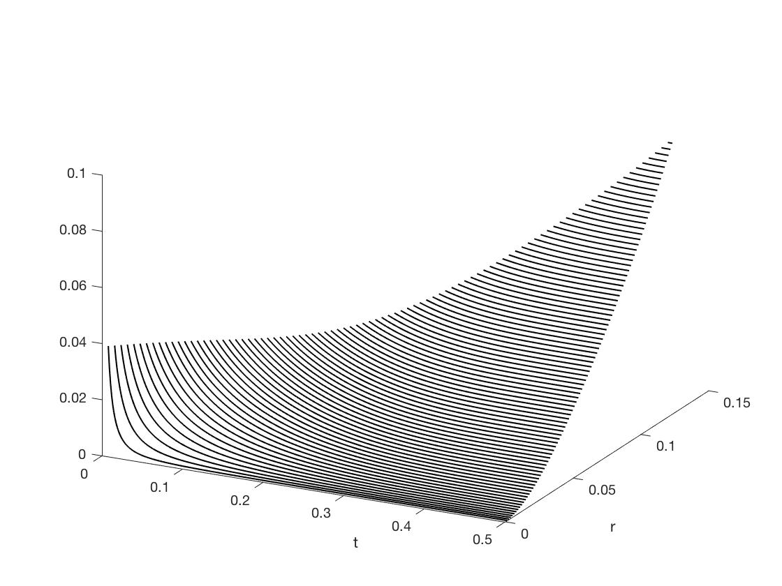
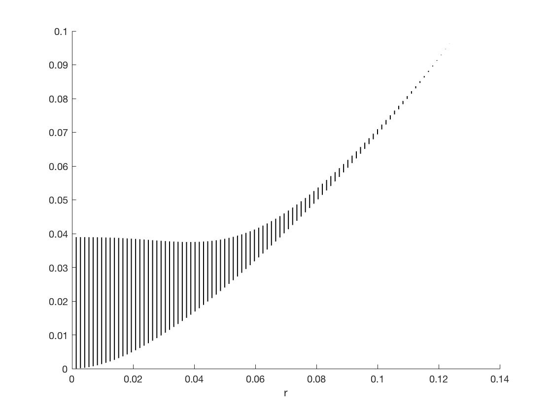
Figure 2: Two views of the graph of the function  $\frac{1}{4}-S(t,r)$ on the triangle $0\leq t\leq\frac{1}{2}$, $0\leq r\leq\frac{1}{4}t$. Note that $S(t,r)$ is multi-valued at $t=r=0$.

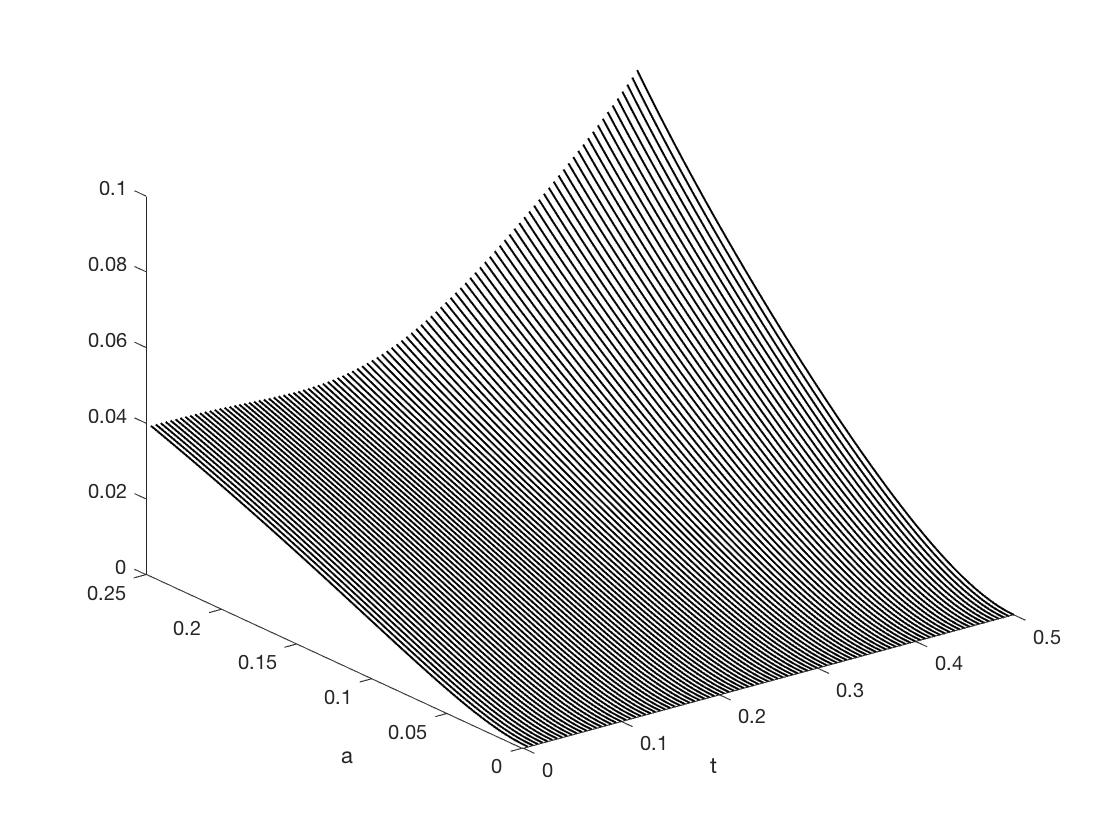
Figure 3: A view of the graph of the function  $\frac{1}{4}-\sigma(t,a)$ in the rectangle $0\leq t\leq\frac{1}{2},0\leq a\leq\frac{1}{4}.$

With the help of a symbolic manipulator, we obtain, for all $t\in[0,\tfrac{1}{2}]$,

$$\sigma(t,0)=\frac{1}{4},\qquad\frac{\partial\sigma}{\partial a}(t,0)=0,\qquad\frac{\partial^{2}\sigma}{\partial a^{2}}(t,0)=-\frac{G(t)}{\tau^{2}},$$

where

$$G(t):=3t^{10}+9t^{8}\tau^{2}-8t^{7}\tau^{3}+16t^{6}\tau^{4}+24t^{5}\tau^{5}+16t^{4}\tau^{6}-8t^{3}\tau^{7}+9t^{2}\tau^{8}+3\tau^{10}.$$

We note that the polynomial $G(t)$ is strictly decreasing in $[0,\frac{1}{2}]$ between $G(0)=3$ and $G(\frac{1}{2})=1$. We thus easily see that $\frac{\partial^{2}\sigma}{\partial a^{2}}(t,0)\leq-1$ for $0\leq t\leq\frac{1}{2}$; hence, by continuity we get the existence of two constants $C_{*}>0$ and $a_{*}\in(0,\tfrac{1}{4}]$ such that $\frac{\partial^{2}\sigma}{\partial a^{2}}(t,a)\leq-C_{*}$ for $0\leq t\leq\frac{1}{2}$ and $0\leq a\leq a_{*}$. With these constants at hand, by Taylor’s expansion with Lagrange’s reminder, we are entitled to write

$$\sigma(t,a)\,=\,\frac{1}{4}+\frac{\partial^{2}\sigma}{\partial a^{2}}(t,\bar{a})a^{2}\,\leq\,\frac{1}{4}-C_{*}a^{2}\qquad\text{for \ }0\leq t\leq\tfrac{1}{2},\ 0<a\leq a_{*},$$

with some $\bar{a}=\bar{a}(t,a)\in(0,a)$.

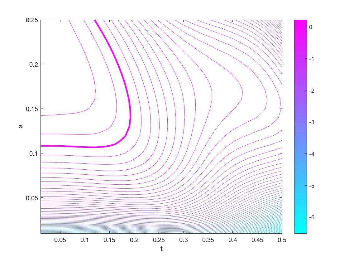
Figure 4: Contour plot of $\frac{\partial^{2}\sigma}{\partial a^{2}}(t,a)$: the function is negative on $[0,\frac{1}{2}]\times[0,a^{*}]$ with $a^{*}>\frac{1}{10}$. The thicker curve represents the zero level set

By computing the symbolic expression of the function $\frac{\partial^{2}\sigma}{\partial a^{2}}(t,a)$ and by examining its level sets (via a numerical procedure), one finds that $a_{*}$ safely satisfies $a_{*}>\frac{1}{10}$ (see Figure 4). Therefore, going back to our function $S(t,r)=\sigma(t,\frac{r}{t})$, we deduce that

$$S(t,r)\leq\frac{1}{4}-\frac{C_{*}}{t^{2}}r^{2}\leq\frac{1}{4}-4C_{*}r^{2}\qquad\text{for \ }0<r\leq\tfrac{1}{10}t,\ \ t\leq\tfrac{1}{2}.$$

Recalling (6.5) and using the expressions $t=4r(i-1)$ and $r=\frac{1}{2}\,\frac{1}{j-4}>\frac{1}{2j}$, we immediately obtain

$${\sf s}_{i}^{(j)}\leq\frac{1}{4}-\frac{C_{*}}{j^{2}}\qquad\text{for \ }4\leq i\leq\tfrac{n}{2}.$$ (6.6)

Note that we require the restriction $i\geq 4$ to satisfy the constraint

$$r\leq\frac{1}{10}t=\frac{2}{5}r(i-1)\qquad\Rightarrow\qquad i\geq\frac{7}{2}.$$

Therefore, we are left with the task of establishing a similar bound for ${\sf s}_{2}^{(j)}$ and ${\sf s}_{3}^{(j)}$ by different means. It is easily checked that for $j\to\infty$ it holds ${\sf s}_{2}^{(j)}\to\frac{65}{308}<\frac{1}{4}$ and ${\sf s}_{3}^{(j)}\to\frac{55}{220}<\frac{1}{4}$, while both ${\sf s}_{2}^{(j)}$ and ${\sf s}_{2}^{(j)}$ are $<\frac{1}{4}$ for all $j\geq 8$. This implies the desired bound for a suitable constant $C_{**}>0$.

The proof of (6.4) is thus complete, whence Proposition 2.2 is established.

References

- [1] I. Babuška, A. Craig, J. Mandel, and J. Pitkäranta. Efficient preconditioning for the p-version finite element method in two dimensions. SIAM J. Numer. Anal., 28(3):624Ж661, 1991.
- [2] R.E. Bank and A. Weiser. Some a posteriori error estimators for elliptic partial differential equations Math. Comp., 44:285–301, 1985.
- [3] F. A. Bornemann, B. Erdmann, and R. Kornhuber, A posteriori error estimates for elliptic problems in two and three space dimensions, SIAM J. Numer. Anal., 33:1188–1204, 1996.
- [4] M. Bürg and W. Dörfler. Convergence of an adaptive finite element strategy in higher space-dimensions. Appl. Numer. Math., 61(11):1132–1146, 2011.
- [5] P. Binev, W. Dahmen, and R. DeVore. Adaptive finite element methods with convergence rates. Numer. Math., 97(2):219 – 268, 2004.
- [6] P. Binev. Tree approximation for -adaptivity. IMI Preprint Series 2015:07, 2015.
- [7] D. Braess, V. Pillwein, and J. Schöberl. Equilibrated residual error estimates are -robust. Comput. Methods Appl. Mech. Engrg., 198(13-14):1189–1197, 2009.
- [8] C. Canuto, M. Y.Hussaini, A. Quarteroni, and T. A. Zang. Spectral Methods. Fundamentals in Single Domains. Springer 2016.
- [9] C. Canuto, R.H. Nochetto, R. Stevenson, and M. Verani. Convergence and optimality of -AFEM. Numer. Math. 135 (2017), 1073-1119
- [10] C. Canuto, R.H. Nochetto, R. Stevenson, and M. Verani. On -robust saturation for -AFEM. Comput. & Math. with Appl. 73 (2017), 2004–2022.
- [11] L. Demkowicz, J. Gopalakrishnan, and J. Schöberl. Polynomial extension operators. Part III. Math. Comp., 81(279):1289–1326, 2012.
- [12] W. Dörfler and R.H. Nochetto, Small data oscillation implies the saturation assumption. Numer. Math. 91:1–12, 2002.
- [13] A. Ern and M. Vohralík. Polynomial-degree-robust a posteriori estimates in a unified setting for conforming, nonconforming, discontinuous Galerkin, and mixed discretizations. SIAM J. Numer. Anal., 53(2):1058–1081, 2015.
- [14] A. Ern and M. Vohralík. Stable broken H1 and H(div) polynomial extensions for polynomial-degree-robust potential and flux reconstruction in three space dimensions. hal 01422204, Inria Paris-Rocquencourt, 2016.
- [15] B. Guo and I. Babuška. The version of finite element method, Part 1: The basic approximation results. Comp. Mech, 1:21–41, 1986.
- [16] B. Guo and I. Babuška. The version of finite element method, Part 2: General results and application. Comp. Mech, 1:203–220, 1986.
- [17] J. M. Melenk and B. I. Wohlmuth. On residual-based a posteriori error estimation in -FEM. Adv. Comput. Math., 15(1-4):311–331, 2002.
- [18] R.H. Nochetto, Removing the saturation assumption in a posteriori error analysis, Istit. Lombardo Accad. Sci. Lett. Rend. A, 127:67-82, 1993.