$B$- and $D$-meson leptonic decay constants from
four-flavor lattice QCD

Abstract

We calculate the leptonic decay constants of heavy-light pseudoscalar mesons with charm and bottom quarks in lattice quantum chromodynamics on four-flavor QCD gauge-field configurations with dynamical $u$, $d$, $s$, and $c$ quarks. We analyze over twenty isospin-symmetric ensembles with six lattice spacings down to $a\approx 0.03$ fm and several values of the light-quark mass down to the physical value $\frac{1}{2}(m_{u}+m_{d})$. We employ the highly-improved staggered-quark (HISQ) action for the sea and valence quarks; on the finest lattice spacings, discretization errors are sufficiently small that we can calculate the $B$-meson decay constants with the HISQ action for the first time directly at the physical $b$-quark mass. We obtain the most precise determinations to-date of the $D$- and $B$-meson decay constants and their ratios, $f_{D^{+}}=212.7(0.6)$ MeV, $f_{D_{s}}=249.9(0.4)$ MeV, $f_{D_{s}}/f_{D^{+}}=1.1749(16)$, $f_{B^{+}}=189.4(1.4)$ MeV, $f_{B_{s}}=230.7(1.3)$ MeV, $f_{B_{s}}/f_{B^{+}}=1.2180(47)$, where the errors include statistical and all systematic uncertainties. Our results for the $B$-meson decay constants are three times more precise than the previous best lattice-QCD calculations, and bring the QCD errors in the Standard-Model predictions for the rare leptonic decays $\overline{\mathcal{B}}(B_{s}\to\mu^{+}\mu^{-})=3.64(11)\times 10^{-9}$, $\overline{\mathcal{B}}(B^{0}\to\mu^{+}\mu^{-})=1.00(3)\times 10^{-10}$, and $\overline{\mathcal{B}}(B^{0}\to\mu^{+}\mu^{-})/\overline{\mathcal{B}}(B_{s}\to\mu^{+}\mu^{-})=0.0273(9)$ to well below other sources of uncertainty. As a byproduct of our analysis, we also update our previously published results for the light-quark-mass ratios and the scale-setting quantities $f_{p4s}$, $M_{p4s}$, and $R_{p4s}$. We obtain the most precise lattice-QCD determination to date of the ratio $f_{K^{+}}/f_{\pi^{+}}=1.1950(^{+16}_{-23})$ MeV.

I Introduction

Leptonic decays of $B$ and $D$ mesons are important probes of heavy-to-light quark flavor-changing interactions. The charged-current decays $H^{+}\to\ell^{+}\nu_{\ell}$ ($H=D^{+},D_{s},B^{+}$; $\ell=e,\mu,\tau$) proceed at tree level in the Standard Model via the axial-vector current $\mathcal{A}_{\mu}\equiv\overline{Q}\gamma_{5}\gamma_{\mu}q$, where $Q$ is the heavy charm or bottom quark and $q$ is the light quark in the pseudoscalar meson. When combined with a nonperturbative lattice-QCD calculation of the decay constant $f_{H^{+}}$, an experimental measurement of the leptonic decay width allows the determination of the corresponding Cabibbo-Kobayashi-Maskawa (CKM) quark-mixing matrix element $|V_{Qq}|$. Because the decays $H^{0}\to\ell^{+}\ell^{-}$ ($H=D^{0},B^{0},B_{s}$) proceed via a flavor-changing-neutral-current interaction, and are forbidden at tree level in the Standard Model, these processes may be especially sensitive to (tree-level) contributions of new heavy particles. Both the Standard-Model and new-physics predictions for the rare-decay branching ratios depend upon the decay constants $f_{H^{0}}$.

Leptonic $B$-meson decays, in particular, make possible several interesting tests of the Standard Model and promising new-physics searches. The determination of $|V_{ub}|$ from $B^{+}\to\tau^{+}\nu_{\tau}$ decay can play an important role in resolving the 2–3$\sigma$ tension between the values of $|V_{ub}|$ obtained from inclusive and exclusive semileptonic $B$-meson decays (see the recent reviews Amhis et al. (2017a); Hamilton et al. (2017) and references therein). Alternatively, the decay $B^{+}\to\tau^{+}\nu_{\tau}$, because of the large $\tau$-lepton mass, may receive observable contributions from new heavy particles such as charged Higgs bosons or leptoquarks Hou (1993); Akeroyd and Recksiegel (2003). The branching ratios for $B^{0}\to\ell^{+}\ell^{-}$ and $B_{s}\to\ell^{+}\ell^{-}$ can be enhanced with respect to the Standard-Model rates in new-physics scenarios with tree-level flavor-changing-neutral currents, such as in fourth-generation models Buras et al. (2013); Buras (2010).

Lattice-QCD calculations of the $B$-meson decay constants are especially timely given the wealth of leptonic $B$-decay measurements from the $B$-factories and, more recently, by hadron-collider experiments at the LHC. The branching ratio for the charged-current decay $B^{+}\to\tau^{+}\nu_{\tau}$ has been measured by the BaBar and Belle experiments to about 20% precision Aubert et al. (2010); Lees et al. (2013); Adachi et al. (2013); Kronenbitter et al. (2015). The rare decay $B_{s}\to\mu^{+}\mu^{-}$ has now been independently observed by the ATLAS, CMS, and LHCb experiments with errors on the measured branching ratio ranging from around 20%–100% Khachatryan et al. (2015); Aaboud et al. (2016); Aaij et al. (2017a); these works have also set limits on the process $B^{0}\to\mu^{+}\mu^{-}$. Precise determinations of $f_{B^{+}}$, $f_{B^{0}}$, and $f_{B_{s}}$ are needed to interpret these results. Such determinations are also necessary to fully exploit coming measurements by Belle II Bennett (2016), which will begin running at the Super-KEKb facility next year, as well as future measurements by ATLAS, CMS, and LHCb after the LHC luminosity and detector upgrades Schmidt (2016), which are planned for 2023–2025. Bazavov et al. (2014a); *Bazavov:2014lja

Several independent three- and four-flavor calculations of heavy-light-meson decay constants using different lattice actions are available Davies et al. (2010); McNeile et al. (2012); Bazavov et al. (2012); Na et al. (2012a, b); Dowdall et al. (2013a); Christ et al. (2015); Bazavov et al. (2014a); Yang et al. (2015); Carrasco et al. (2015a); Bussone et al. (2016); Boyle et al. (2017); Hughes et al. (2018), with uncertainties ranging from $\sim 0.5\%$–5% and $\sim 2\%$–8% for the $D_{(s)}$ and $B_{(s)}$ systems, respectively. The most precise results for $f_{D}$ and $f_{D_{s}}$ have been obtained by us Bazavov et al. (2014a); *Bazavov:2014lja, and for $f_{B_{s}}$ by the HPQCD Collaboration McNeile et al. (2012), in both cases using improved staggered sea quarks and the “highly-improved staggered quark” (HISQ) action Follana et al. (2007) for the valence light and heavy quarks. The HISQ action makes possible this high precision because it has both small discretization errors, even at relatively large lattice spacings, and an absolutely-normalized axial current. Our previous calculation Bazavov et al. (2014a); *Bazavov:2014lja of the $D_{(s)}$-meson decay constants employed physical-mass light and charm quarks and gauge-field configurations with lattice spacings down to $a\approx 0.06$ fm; the dominant contribution to the errors on $f_{D}$ and $f_{D_{s}}$ came from the continuum extrapolation. HPQCD’s calculation of $f_{B_{s}}$ with the HISQ action for the $b$ quark employed five three-flavor ensembles of gauge-field configurations from the MILC Collaboration Bernard et al. (2001); Aubin et al. (2004); Bazavov et al. (2010a) with lattice spacings as fine as $a\approx 0.045$ fm, enabling them to simulate with heavy-quark masses close to the physical bottom-quark mass. The statistical errors dominate in their calculation due to the comparatively small number of configurations per ensemble (roughly 200 on their finest up to 600 on their coarsest). Other important sources of uncertainty are from the extrapolation in heavy-quark mass up to $m_{b}$ and from the extrapolation to zero lattice spacing.

In this paper, we present a new calculation of the leptonic decay constants of heavy-light mesons containing bottom and charm quarks that improves upon prior works in several ways. As in our previous calculation of $f_{D}$ and $f_{D_{s}}$ Bazavov et al. (2014a); *Bazavov:2014lja, we employ the four-flavor QCD gauge-field configurations generated by the MILC Collaboration with HISQ up, down, strange, and charm quarks Bazavov et al. (2013); we also use the HISQ action for the light and heavy valence quarks. We now employ three new ensembles with finer lattice spacings of $a\approx 0.042$ and $a\approx 0.03$ fm, and also increase statistics on the $a\approx 0.06$ fm ensemble with physical-mass light quarks. Altogether, we analyze 24 ensembles, most of which have approximately 1000 configurations. We also calculate the $B^{+}$- and $B^{0}$-meson decay constant with HISQ $b$ quarks on the HISQ ensembles for the first time.

We fit our lattice data for the heavy-light meson decay constants to a functional form that combines information on the heavy-quark mass dependence from heavy-quark effective theory, on the light-quark mass dependence from chiral perturbation theory, and on discretization effects from Symanzik effective theory. This allows us to exploit our wide range of simulation parameters by including multiple lattice spacings and heavy- and light-quark mass values in a single effective-field-theory (EFT) fit. We present results for all charged and neutral heavy-light pseudoscalar-meson decay constants, as well as the SU(3)-breaking decay-constant ratios and the differences between the charged decay constants and the decay constants in the isospin-symmetric ($m_{u}=m_{d}$) limit. In addition, we provide the correlations between our decay-constant results to facilitate their use in other phenomenological studies beyond this work. Preliminary reports of this analysis have been presented in Refs. Bazavov et al. (2016a); Komijani et al. (2016).

This paper is organized as follows. First, Sec. II presents relevant details of the lattice actions, simulation parameters, and methodology of our calculation, including a discussion of how we deal with nonequilibrated topological charge. Next, we describe our two-point correlator fits used to obtain the heavy-light-meson decay amplitudes in Sec. III. In Sec. IV, we determine the lattice spacings and light-quark masses on the ensembles employed in this calculation, which are parametric inputs to the decay-constant analysis, and also to a determination of heavy-quark masses in a companion paper Bazavov et al. (2018). Physical quark-mass ratios and the light decay constant ratio $f_{K^{+}}/f_{\pi^{+}}$ are obtained as a byproduct. We then calculate the physical $B$- and $D$-meson decay-constant values in Sec. V by fitting our lattice decay-amplitude data at multiple values of the light- and heavy-quark masses and lattice spacing to a function based on effective field theories, and interpolating to the physical light-, charm-, and bottom-quark masses and extrapolating to the continuum limit. In Sec. VI, we estimate the systematic uncertainties in the decay constants not included in the EFT fit, and provide complete error budgets. We present our final results for the $B$- and $D$-meson leptonic decay constants with total errors and discuss the impact of our results for determinations of CKM matrix elements and tests of the Standard Model in Sec. VII. Final results for light-quark mass ratios, $f_{K^{+}}/f_{\pi^{+}}$, and the scale-setting quantities $f_{p4s}$ and $M_{p4s}$ are also presented. Finally, in Sec. VIII, we conclude with an outlook to future work. Two appendices provide useful information about (improved) staggered fermions when the bare lattice quark mass $am_{0}\not\ll 1$. Appendix A discusses the radius of convergence of the expansion in $am_{0}$, while Appendix B derives the normalization factor for staggered bilinears. Appendix C provides the correlation and covariance matrices between our $B$- and $D$-meson decay constant results.

II Simulation Parameters and Methods

In this paper, we use the MILC Collaboration’s ensembles of QCD gauge-field configurations with four flavors of dynamical quarks. This simulation program is described in detail in Ref. Bazavov et al. (2013), and since then it has been extended to smaller lattice spacings. Here we provide information on our current calculation, and also document the new ensembles. First, in Sec. II.1, we summarize the parameters of the actions and two-point correlation functions used in the analysis presented below. Three ensembles with approximate lattice spacings 0.042 and 0.03 fm are new since Ref. Bazavov et al. (2013), while some of the older ensembles have been extended. In Sec. II.2, we update the discussion in Ref. Bazavov et al. (2013) on possible effects from using different algorithms in different parts of the simulation. Finally, in Sec. II.3, we discuss effects of poor sampling of the distribution of topological charge and how to compensate for these effects.

II.1 Simulation parameters

The gauge action Weisz (1983); *Weisz:1983bn; *Curci:1983an; *Luscher:1985zq; *Luscher:1984xn; *Alford:1995hw; *Hart:2008sq is one-loop Symanzik Symanzik (1980); *Symanzik:1983dc and tadpole Lepage and Mackenzie (1993) improved, using the plaquette to determine the tadpole quantity $u_{0}$. The fermion action is the HISQ action introduced by the HPQCD collaboration Follana et al. (2007). The ensembles all have an isospin-symmetric sea. A single staggered-fermion field yields four species, known as tastes, in the continuum limit Karsten and Smit (1981). To adjust the number of species in the sea, we take the fourth (square) root of the quark determinant for the strange and charm (up and down) sea Marinari et al. (1981). In addition to the perturbative arguments Karsten and Smit (1981); Giedt (2007), this procedure passes several nonperturbative tests Follana et al. (2004); Dürr et al. (2004); Dürr and Hoelbling (2005); Wong and Woloshyn (2005); Shamir (2005); Prelovsek (2006); Bernard (2006); Dürr and Hoelbling (2006); Bernard et al. (2006); Shamir (2007); Bernard et al. (2007); Kronfeld (2007); Donald et al. (2011), providing confidence that continuum QCD is obtained as $a\to 0$.

Table 1 summarizes the ensembles used in this work.

Table 1: Ensembles used in this calculation. The notation and symbols are discussed in the text. In the first column the approximate lattice spacings are mnemonic only; the precise values are tabulated in Table 9. The second column is used as a key to identify the ensembles at a given approximate lattice spacing. A dagger ($\dagger$) on $am^{\prime}_{s}$ flags ensembles for which the simulation strange-quark mass is deliberately chosen far from the physical value. The $M_{\pi}$ and $L$ values are different from those listed in Table I of Ref. Bazavov et al. (2014a), because those values assumed a mass-dependent scale setting scheme.

$\approx a$	Key	$\beta$	$am^{\prime}_{l}$	$am^{\prime}_{s}$	$am^{\prime}_{c}$	$(L/a)^{3}$$\times$	$(T/a)$	$L$	$M_{\pi}$	$M_{\pi}L$	$N_{\text{conf}}$
(fm)								(fm)	(MeV)
0.15	$m_{s}/5$	5.80	0.013	0.065	0.838	$16^{3}$$\times$	$48$	2.45	305	3.8	1020
0.15	$m_{s}/10$	5.80	0.0064	0.064	0.828	$24^{3}$$\times$	$48$	3.67	214	4.0	1000
0.15	physical	5.80	0.00235	0.0647	0.831	$32^{3}$$\times$	$48$	4.89	131	3.3	1000
0.12	$m_{s}/5$	6.00	0.0102	0.0509	0.635	$24^{3}$$\times$	$64$	2.93	305	4.5	1040
0.12	unphysA	6.00	0.0102	0.03054†	0.635	$24^{3}$$\times$	$64$	2.93	304	4.5	1020
0.12	small	6.00	0.00507	0.0507	0.628	$24^{3}$$\times$	$64$	2.93	218	3.2	1020
0.12	$m_{s}/10$	6.00	0.00507	0.0507	0.628	$32^{3}$$\times$	$64$	3.91	217	4.3	1000
0.12	large	6.00	0.00507	0.0507	0.628	$40^{3}$$\times$	$64$	4.89	216	5.4	1028
0.12	unphysB	6.00	0.01275	0.01275†	0.640	$24^{3}$$\times$	$64$	2.93	337	5.0	1020
0.12	unphysC	6.00	0.00507	0.0304†	0.628	$32^{3}$$\times$	$64$	3.91	215	4.3	1020
0.12	unphysD	6.00	0.00507	0.022815†	0.628	$32^{3}$$\times$	$64$	3.91	214	4.2	1020
0.12	unphysE	6.00	0.00507	0.012675†	0.628	$32^{3}$$\times$	$64$	3.91	214	4.2	1020
0.12	unphysF	6.00	0.00507	0.00507†	0.628	$32^{3}$$\times$	$64$	3.91	213	4.2	1020
0.12	unphysG	6.00	0.0088725	0.022815†	0.628	$32^{3}$$\times$	$64$	3.91	282	5.6	1020
0.12	physical	6.00	0.00184	0.0507	0.628	$48^{3}$$\times$	$64$	5.87	132	3.9	2999
0.09	$m_{s}/5$	6.30	0.0074	0.037	0.440	$32^{3}$$\times$	$96$	2.81	316	4.5	1005
0.09	$m_{s}/10$	6.30	0.00363	0.0363	0.430	$48^{3}$$\times$	$96$	4.22	221	4.7	2999
0.09	physical	6.30	0.0012	0.0363	0.432	$64^{3}$$\times$	$96$	5.62	129	3.7	2484
0.06	$m_{s}/5$	6.72	0.0048	0.024	0.286	$48^{3}$$\times$	$144$	2.72	329	4.5	1016
0.06	$m_{s}/10$	6.72	0.0024	0.024	0.286	$64^{3}$$\times$	$144$	3.62	234	4.3	2572
0.06	physical	6.72	0.0008	0.022	0.260	$96^{3}$$\times$	$192$	5.44	135	3.7	2842
0.042	$m_{s}/5$	7.00	0.00316	0.0158	0.188	$64^{3}$$\times$	$192$	2.73	315	4.3	1167
0.042	physical	7.00	0.000569	0.01555	0.1827	$144^{3}$$\times$	$288$	6.13	134	4.2	2420
0.03	$m_{s}/5$	7.28	0.00223	0.01115	0.1316	$96^{3}$$\times$	$288$	3.09	309	4.8	2724

In this table, we identify the ensembles by the approximate lattice spacing $a$ and the ratio of light sea-quark ($m^{\prime}_{l}$) to strange sea-quark mass ($m^{\prime}_{s}$). The exact lattice spacing and physical strange-quark mass ($m_{s}$) are outputs of our decay-constant analysis and can be found in Table 9 in Sec. V. The six lattice spacings range from approximately $0.15$ fm to $0.03$ fm, and the sea has light sea-quark masses $0.2m^{\prime}_{s}$, $0.1m^{\prime}_{s}$, and approximately physical. In most ensembles, $m^{\prime}_{s}$ is chosen close to the physical strange-quark mass, but sometimes it is deliberately chosen far from physical to provide useful information about the sea-quark-mass dependence. In all ensembles, the charm-quark mass is chosen close to its physical value. In Table 1, $\beta=10/g^{2}$ is the gauge coupling, $T$ and $L$ are the lattice temporal and spatial extents, and $M_{\pi}$ is the mass of the taste-Goldstone sea pion.

For each ensemble, the light, strange, and charm sea-quark masses are estimated either from short tuning runs or from tuned masses on nearby ensembles. These values are always found to be slightly in error once higher statistics become available, so it is necessary to adjust for this small sea-quark-mass mistuning a posteriori, as we do in the fitting procedure described in Sec. V.

Table 2: Valence-quark masses used in each ensemble. The first two columns identify the ensemble. The third column gives the lightest valence-quark mass in units of the sea strange-quark mass. (The full set of light valence-quark masses is listed in the text.) The fourth column shows the heavy valence-quark masses in units of the sea charm-quark mass. The last column shows the number of configurations and the number of source time slices used on each.

$\approx a$ (fm)	Key	$m_{\text{min}}/m^{\prime}_{s}$	$m_{h}/m^{\prime}_{c}$	$N_{\text{conf}}$$\,\times\,$	$N_{\text{src}}$
0.15	$m_{s}/5$	0.1n7	{0.9, 1.0}	1020$\,\times\,$	4
0.15	$m_{s}/10$	0.1n7	{0.9, 1.0}	1000$\,\times\,$	4
0.15	physical	0.037	{0.9, 1.0}	1000$\,\times\,$	4
0.12	$m_{s}/5$	0.1n7	{0.9, 1.0}	1040$\,\times\,$	4
0.12	unphysA	0.1n7	{0.9, 1.0}	1020$\,\times\,$	4
0.12	small	0.1n7	{0.9, 1.0}	1020$\,\times\,$	4
0.12	$m_{s}/10$	0.1n7	{0.9, 1.0}	1000$\,\times\,$	4
0.12	large	0.1n7	{0.9, 1.0}	1028$\,\times\,$	4
0.12	unphysB	0.1n7	{0.9, 1.0}	1020$\,\times\,$	4
0.12	unphysC	0.1n7	{0.9, 1.0}	1020$\,\times\,$	4
0.12	unphysD	0.1n7	{0.9, 1.0}	1020$\,\times\,$	4
0.12	unphysE	0.1n7	{0.9, 1.0}	1020$\,\times\,$	4
0.12	unphysF	0.1n7	{0.9, 1.0}	1020$\,\times\,$	4
0.12	unphysG	0.1n7	{0.9, 1.0}	1020$\,\times\,$	4
0.12	physical	0.037	{0.9, 1.0}	999$\,\times\,$	4
0.09	$m_{s}/5$	0.1n7	{0.9, 1.0}	1005$\,\times\,$	4
0.09	$m_{s}/10$	0.1n7	{0.9, 1.0}	999$\,\times\,$	4
0.09	physical	0.033	{0.9, 1.0, 1.5, 2.0, 2.5, 3.0}	484$\,\times\,$	4
0.06	$m_{s}/5$	0.057	{0.9, 1.0}	1016$\,\times\,$	4
0.06	$m_{s}/10$	0.057	{0.9, 1.0, 2.0, 3.0, 4.0}	572$\,\times\,$	4
0.06	physical	0.036	{0.9, 1.0, 1.5, 2.0, 2.5, 3.0, 3.5, 4.0, 4.5}	842$\,\times\,$	6
0.042	$m_{s}/5$	0.036	{0.9, 1.0, 1.5, 2.0, 2.5, 3.0, 3.5, 4.0, 4.5}	1167$\,\times\,$	6
0.042	physical	0.037	{0.9, 1.0, 1.5, 2.0, 2.5, 3.0, 3.5, 4.0, 4.5, 5.0}	420$\,\times\,$	6
0.03	$m_{s}/5$	0.257	{0.9, 1.0, 1.5, 2.0, 2.5, 3.0, 3.5, 4.0, 4.5, 5.0}	724$\,\times\,$	4

We compute pseudoscalar correlators for several valence-quark masses on each ensemble. In almost all cases, we use light valence-quark masses of $0.1m^{\prime}_{s}$, $0.2m^{\prime}_{s}$, $0.3m^{\prime}_{s}$, $0.4m^{\prime}_{s}$, $0.6m^{\prime}_{s}$, $0.8m^{\prime}_{s}$ and $1.0m^{\prime}_{s}$, where the prime distinguishes the strange sea-quark mass from the post-production, better-tuned mass. To save computer time, however, for the finest ensemble with $a\approx 0.03$ fm and $m^{\prime}_{l}=m^{\prime}_{s}/5$, we only use valence-quark masses greater than or equal to the light sea-quark mass $0.2m^{\prime}_{s}$. For the physical quark-mass ensembles and the ensembles with $a\approx 0.06$ and 0.042 fm, we use lighter valence-quark masses, usually going down to the estimated physical light-quark mass. The wide range of valence-quark masses on the ensembles with $a\geq 0.042$ fm are used to determine the light-quark-mass dependence, while the 0.03 fm ensemble helps guide the continuum limit. This strategy saves computer time, since light-quark propagators on these lattices are expensive, the cost being approximately proportional to $1/am_{q}$. In all cases, we compute valence heavy-quark propagators with masses of $1.0m^{\prime}_{c}$ and $0.9m^{\prime}_{c}$, to allow interpolation or extrapolation to the physical charm-quark mass. Finally, on six of the ensembles we use valence-quark masses heavier than charm to allow us to extrapolate, and on the finest lattices interpolate, to the $b$-quark mass. Table 2 shows the lightest valence-quark mass used on each ensemble in units of the strange sea-quark mass, and also the heavy-quark masses used on each ensemble.

On each configuration, we compute quark propagators from four or six evenly-spaced source time slices. We change the location of the first source time slice from configuration to configuration, shifting by an amount approximately equal to half the spacing between source time slices but incommensurate with the lattice size, so that all possible source locations are used. Table 2 also shows the number of source time slices used on each ensemble.

II.2 RHMC and RHMD algorithms

The coarser ensembles were all generated using the rational hybrid Monte Carlo (RHMC) algorithm Duane (1985); Duane and Kogut (1986); Gottlieb et al. (1987); Sexton and Weingarten (1992); Kennedy et al. (1999); Hasenbusch (2001); Omelyan et al. (2002); Clark and Kennedy (2007); Takaishi and de Forcrand (2006); Duane et al. (1987), but some of the finer ensembles were generated with a mixture of the RHMC and the rational hybrid molecular dynamics (RHMD) Duane (1985); Duane and Kogut (1986); Gottlieb et al. (1987); Sexton and Weingarten (1992); Kennedy et al. (1999); Hasenbusch (2001); Omelyan et al. (2002); Clark and Kennedy (2007); Takaishi and de Forcrand (2006); Bazavov et al. (2010a, 2013) algorithms. The two most recently generated ensembles, one with $a\approx 0.042$ fm and physical light-quark mass and another with $a\approx 0.03$ fm and $m^{\prime}_{l}=m^{\prime}_{s}/5$, were generated entirely with the RHMD algorithm. The considerations behind these choices, and the effects of using the RHMD algorithm, are discussed in detail in Ref. Bazavov et al. (2013). Since the preparation of Ref. Bazavov et al. (2013), three of the ensembles have been enlarged, which enables us to update the comparison of the RHMC and RHMD algorithms in that work.

Table 3 shows the differences in the plaquettes between the parts of the ensembles generated with RHMC and RHMD algorithms for the ensembles where both algorithms were used. The numbers of configurations used in this comparison differ from those in Table 1 because heavier-than-charm correlators were only run on parts of the first two ensembles listed, and the third ensemble was extended slightly after this comparison was done. In addition, the plaquette was measured after every trajectory, giving 2–3 times larger statistics than used in our decay-constant calculation. Motivated by the expectation that using an approximate integration procedure amounts to simulating with a slightly different action, we can estimate the importance of these shifts by asking how much the bare coupling or, equivalently, the lattice spacing would need to be adjusted to change the average plaquette by this amount. From looking at the plaquette at a couple of lattice spacings, we find $\Delta\ln(a)/\Delta\,\text{plaq}\approx-4.2$, which leads to the corresponding values of ${\Delta a}/{a}$ given in the final column of Table 3. Clearly, these differences are quite small. In fact, they are negligible, because in the analysis reported below we use $f_{\pi}$ to set the scale, and the fractional error on the current value for $f_{\pi}$ from the Particle Data Group (PDG) Patrignani et al. (2016); Rosner et al. (2015) is about $150\times 10^{-5}$.

Table 3: Results for the plaquette from the RHMC and RHMD algorithms. The first two columns give the approximate lattice spacing and the ratio of the light- to strange sea-quark masses. The third and fourth columns give the time-step sizes used with the RHMC and RHMD algorithms, respectively, while the fifth and sixth columns give the simulation time multiplied by the acceptance rate for the two algorithms; the “effective time units”, which is the molecular dynamics time multiplied by the acceptance rate, indicates the amount of data used in each measurement. The seventh column is the difference in the plaquette, $\Delta(\text{plaq})$, from the two algorithms. and the last column the fractional change in the lattice spacing, $\Delta a/a$, needed to create such a difference in the plaquette.

$\approx a$ (fm)	$m^{\prime}_{l}/m^{\prime}_{s}$	RHMC	RHMD	RHMC	RHMD	$\Delta(\text{plaq})$	${\Delta a}/{a}$
		time step		effective time units
0.09	1/27	0.0115	0.0133	1339	2962	$-3.0(5)\times 10^{-5}$	$13\times 10^{-5}$
0.06	1/10	0.0141	0.0143	2703	2180	$-1.2(5)\times 10^{-5}$	1$5\times 10^{-5}$
0.06	1/27	0.0100	0.0125	2288	3432	$-1.1(4)\times 10^{-5}$	1$5\times 10^{-5}$

The new $a\approx 0.042$ fm physical-mass ensemble has the largest physical volume of the four-flavor MILC ensembles, with a spatial size of about 6 fm, while the new $a\approx 0.03$ fm ensemble with $m^{\prime}_{l}/m^{\prime}_{s}=1/5$ has the smallest lattice spacing. When the physical volume is made larger, more low-momentum (long-distance) modes are added to the system. Based on these considerations, we do not expect this added physics to be very sensitive to the molecular dynamics step size. On the other front, the lattice spacing is made smaller by making $\beta$ larger. If the ultraviolet gauge modes are viewed as free fields, the coefficient of the gauge fields in the molecular-dynamics Hamiltonian is proportional to $\beta$ while the coefficient of the conjugate momenta added for the molecular-dynamics time evolution is held fixed. Thus, the frequency of the modes in molecular dynamics time is proportional to $\beta^{1/2}$. Strictly speaking, if we wish to keep the fractional error fixed while increasing $\beta$, we should reduce the step size as $\beta^{-1/2}$. That dependence is very weak—the square root of $\ln a$. It turns out that this scaling is more or less what was chosen empirically in going from $a\approx 0.09$ fm to $0.042$ fm. The step size was decreased from 0.0133 to 0.0125, or by about 6%, as $\beta$ was increased from 6.3 to 7.0, corresponding to $\beta^{1/2}$ changing by 5%.

II.3 Correction for nonequilibrated topological charge

Because QCD simulations use approximately continuous update algorithms, the topological charge $Q$ evolves more and more slowly as the lattice spacing becomes smaller. In our finest ensembles, the evolution has slowed so much that the distribution of $Q$ has not been sampled properly. Time histories of the topological charge in many of the HISQ ensembles can be found in Ref. Bernard and Toussaint (2018). In Fig. 1, we show one case, $a\approx 0.06$ fm and physical $m^{\prime}_{l}$, where the topological charge is well equilibrated, and a second case, $a\approx 0.042$ fm and $m^{\prime}_{l}=m^{\prime}_{s}/5$, where its distribution is clearly not well sampled.

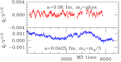
Figure 1: Simulation time history of the topological charge in two cases. The upper panel is for the physical quark mass run at $a\approx 0.06$ fm, and shows a case where the distribution of $Q$ is well sampled. The three sections of the trace correspond to three separate runs with the same parameters. The lower panel, for the $m^{\prime}_{l}=m^{\prime}_{s}/5$ run at $a\approx 0.042$ fm, shows a case where the time history is not well sampled, and where we will apply the correction factors discussed in Ref. Bernard and Toussaint (2018).

As first discussed in Ref. Brower et al. (2003), one can study the $Q$-dependence of observables in chiral perturbation theory ($\chi$PT). Bernard and Toussaint Bernard and Toussaint (2018) recently extended this approach to heavy-light decay constants in the context of heavy-meson $\chi$PT. We use their results to adjust the raw decay-constant results to account at lowest order for the incomplete sampling of $Q$ in the small-$a$ ensembles. The amount of the adjustment is smaller than our statistical errors, but not negligible in comparison to other systematic effects.

We summarize here the key results that allow us to make this adjustment. Let $\Phi_{H_{x}}=f_{H_{x}}\sqrt{M_{H_{x}}}$ be the heavy-light decay constant, in the normalization suitable for heavy quarks. Let $B$ denote either the meson mass $M$, the decay constant $f$, or the combination $\Phi_{H}$. In a finite volume $V$ at fixed $Q$, the masses and decay constants obey Brower et al. (2003); Aoki and Fukaya (2010).

$$B\big{|}_{Q,V}=B+\frac{1}{2\chi_{T}V}B^{\prime\prime}\left(1-\frac{Q^{2}}{\chi_{T}V}\right)+\text{O}\left((\chi_{T}V)^{-2}\right),$$ (1)

where on the right-hand side $B$ is the infinite-volume value, properly averaged over $Q$, $B^{\prime\prime}$ is its second derivative with respect to the vacuum angle $\theta$, evaluated at $\theta=0$, and $\chi_{T}$ is the topological susceptibility

$$\chi_{T}=\frac{\langle Q^{2}\rangle}{V}$$ (2)

in a fully-sampled, large-volume ensemble. For three sea quarks with masses $m_{u}=m_{d}=m_{l}$ and $m_{s}$, light-meson $\chi$PT for the valence-meson mass and decay constant gives Aoki and Fukaya (2010); Bernard and Toussaint (2018)

$$M_{xy}^{\prime\prime} =-M_{xy}\frac{m_{l}^{2}m^{2}_{s}}{2(m_{l}+2m_{s})^{2}}\frac{1}{m_{x}m_{y}},$$ (3)

$$f_{xy}^{\prime\prime} =-f_{xy}\frac{m_{l}^{2}m_{s}^{2}}{4(m_{l}+2m_{s})^{2}}\frac{(m_{x}-m_{y})^{2}}{m^{2}_{x}m^{2}_{y}},$$ (4)

where subscripts $x$ and $y$ denote flavor, and the meson mass and decay constant are at $\theta=0$. A similar calculation in heavy-meson $\chi$PT gives Bernard and Toussaint (2018)

$$\Phi^{\prime\prime}_{H_{x}} =-\Phi_{H_{x}}\frac{m_{l}^{2}m_{s}^{2}}{4(m_{l}+2m_{s})^{2}}\frac{1}{m^{2}_{x}},$$ (5)

$$M^{\prime\prime}_{x} =-2B_{0}\lambda_{1}\frac{m_{l}^{2}m_{s}^{2}}{(m_{l}+2m_{s})^{2}}\frac{1}{m_{x}}-2B_{0}\lambda^{\prime}_{1}\frac{m_{l}m_{s}}{m_{l}+2m_{s}},$$ (6)

where $m_{x}$ is the mass of the light valence quark, and $B_{0}$, $\lambda_{1}$, and $\lambda_{1}^{\prime}$ are low energy constants, which are estimated in a companion paper on heavy-light meson masses Bazavov et al. (2018). These are the appropriate results even with 2+1+1 flavors of sea quark, because the charmed sea quark decouples from the chiral theory. Although the dependence of masses and decay constants are usually small compared to our statistical errors, we have been able to resolve them in some of our well-equilibrated ensembles and confirm, within limited statistics, that our data agree with these formulas Bernard and Toussaint (2016, 2018).

Knowing the dependence of masses and decay constants on the average $Q^{2}$, one can correct the simulation results to account for the difference of the simulation average $\langle Q^{2}\rangle_{\text{sample}}$, and the correct $\langle Q^{2}\rangle$. The lowest order $\chi$PT result for the topological susceptibility is Leutwyler and Smilga (1992)

$$\chi_{T}=\frac{f_{\pi}^{2}}{4}\left(\frac{2}{M_{\pi,I}^{2}}+\frac{1}{M_{ss,I}^{2}}\right)^{-1}\,,$$ (7)

where the effect of staggered taste-violations has been included at leading order by using the taste-singlet meson masses Aubin and Bernard (2003); Billeter et al. (2004), indicated by “$I$.” The correction to the decay constants is then given by

$$f_{\text{corrected}}=f_{\text{sample}}-\frac{1}{2\chi_{T}V}F^{\prime\prime}\left(1-\frac{\langle Q^{2}\rangle_{\text{sample}}}{\chi_{T}V}\right)$$ (8)

with $\chi_{T}$ from Eq. (7).

MILC has calculated $\langle Q^{2}\rangle_{\text{sample}}$ on all ensembles listed in Table 1. For more details, see Ref. Bernard and Toussaint (2018). For three of the finest ensembles, namely those at $a\approx 0.042$ and $0.03$ fm, the simulation time histories of $Q^{2}$ show that it is not well equilibrated. In the analysis below, we use Eq. (8) with $\langle Q^{2}\rangle_{\text{sample}}$ calculated by MILC to adjust the decay-constant data. The adjusted data are used in our central fit, and we take 100% of the difference between fit results with the adjusted data and with the unadjusted data as the systematic error in our results from incomplete equilibration of the topological charge.

III Two-point correlator fits

Our procedures for calculating pseudoscalar meson correlators and for finding masses and amplitudes from these correlators are the same as those used in our earlier computation of charm-meson decay constants in Ref. Bazavov et al. (2014a); *Bazavov:2014lja. Our analysis includes new and extended ensembles, however, so the fit ranges and the number of states employed have been updated.

We compute quark propagators with both “Coulomb-wall” and “random-wall” sources, using four source time slices per gauge-field configuration in most cases, but six source time slices on the $0.042$ fm $m_{s}/5$ ensemble and the $0.06$ and $0.042$ fm physical quark mass ensembles. The pseudoscalar decay constant is obtained from the amplitude of a correlator of a single-point pion operator, $|M^{-1}(x,y)|^{2}$, where $M$ is the lattice fermion matrix $D\kern-6.49994pt/\kern 1.99997pt+m$. The random-wall source consists of a randomly oriented unit vector in color space at each spatial lattice point at the source time. When averaged over sources, contributions to the correlator where the quark and antiquark are on different spatial points average to zero, so the average correlator is just the point-to-point correlator multiplied by the spatial size of the lattice, and the improved statistics from averaging over all the spatial source points more than makes up for the noise introduced from contributions with the quark and antiquark at different spatial points. We use three random source vectors at each source time slice.

For the Coulomb-wall source we fix to the lattice Coulomb gauge, and then use a source in a fixed direction in color space at each spatial lattice point. We use three such vectors, chosen to lie along the three coordinate axes in color space. The Coulomb-wall source is effectively smeared over the whole spatial slice, which we expect to suppress the overlap with excited hadrons, allowing us to use smaller distances in our fits. The Coulomb-wall correlators also have smaller statistical errors. We fit the correlators from the Coulomb-wall and random-wall sources simultaneously with different amplitudes for each source but common masses. The ground-state amplitude from the random-wall source gives the decay constant, but the Coulomb-wall source helps in accurately fixing the ground state mass, which in turn improves the determination of the random-wall amplitude. Figure 2 shows an example of heavy-light pseudoscalar correlators from the $a\approx 0.042$ fm physical quark-mass ensemble for the light-charm and strange-charm masses, showing the smaller excited state contamination in the Coulomb-wall correlator.

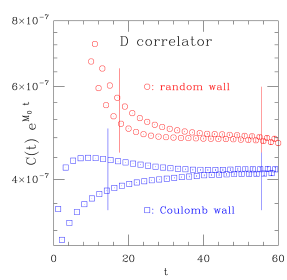
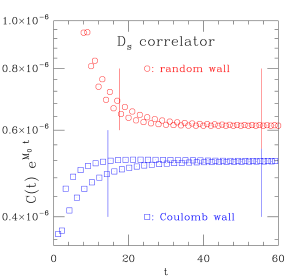
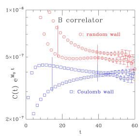
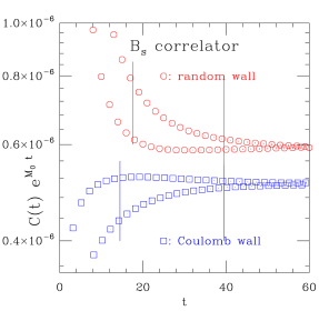
Figure 2: Pseudoscalar correlators for the $D$ (top left), $D_{s}$ (top right), $B$ (bottom left), and $B_{s}$ (bottom right) mesons on the $a\approx 0.042$ fm physical-quark-mass ensemble. Here the valence charm-quark mass is equal to the sea charm-quark mass, and the bottom-quark mass is equal to 4.5 times the charm-quark mass. The red octagons are the random-wall source correlator and the blue squares the Coulomb-wall correlator. Both correlators have been rescaled by $e^{M_{0}T}$ where $M_{0}$ is the ground-state mass; the random-wall correlators have also been multiplied by an arbitrary factor to make the vertical scale convenient. The vertical lines show the fit ranges used in the 3+2 state fits in our analysis. The $D$- and $D_{s}$-meson fits have $p$-values 0.66 and 0.71 respectively, while the $B$- and $B_{s}$-meson fits have $p$-values 0.29 and 0.40 respectively. (The oscillatory behavior in $t$ comes from the positive parity states in the correlator.)

In all cases the sink operator is point-like, with quark and antiquark propagators contracted at each lattice sites. We sum the correlators over all spatial slices to project onto zero three-momentum.

The source time slices are equally spaced throughout the lattice. The location of the first source time slice varies from configuration to configuration by adding an increment close to one half the source separation, but such that all source slices are eventually used. For example, on the $a\approx 0.042$ fm physical quark-mass ensemble, where we use six source time slices with a separation $t/a=48$, the location of the first source time slice on the $N^{\text{th}}$ configuration is $19N$ mod 48, or a shift of 19 slices between successive configurations. Meson masses and decay constants are obtained from fitting to these correlators. For the light-light mesons, we include contributions from the ground state and one opposite parity state in the fit function, taking a large enough minimum distance to suppress excited states. This procedure works well for the light-light pseudoscalars, for which broken chiral symmetry makes the ground state mass much lighter than all the excited state masses.

Because the heavy-light correlators are noisier than the light-light correlators, and the gap in mass between the ground state and excited states is smaller, we include smaller distances and more states in the two-point correlator fits. The fits that yield the central values employed in the subsequent EFT analysis include three states with negative parity (pseudoscalars) and two states with the opposite parity, corresponding to the oscillations in $t$ seen in Fig. 2. We refer to these as “3+2” state fits. For these fits, the minimum distances and fit ranges used vary with the heavy-quark mass. However, they are kept constant in physical units across all ensembles with different sea-quark masses and lattice spacings, subject to being truncated to an integer in lattice units. In these fits, the mass gaps are constrained with Gaussian priors Lepage et al. (2002), but the amplitudes are left unconstrained. Table 4 shows the constraints on the mass gaps used in the heavy-light correlator fits.

Table 4: Bayesian prior constraints on the mass splittings used in our heavy-light correlator fits. Here $M_{0}$ is the ground-state mass, $M_{1}$ and $M_{2}$ are the first and second same-parity excited-state masses, and $M_{0}^{\prime}$ and $M_{1}^{\prime}$ are the ground and first excited-state opposite-parity masses.

$N_{\text{states}}$	$M_{0}^{\prime}-M_{0}$ (MeV)	$M_{1}-M_{0}$ (MeV)	$M_{1}^{\prime}-M_{0}^{\prime}$ (MeV)	$M_{2}-M_{1}$ (MeV)
3+2	$400\pm 200$	$700\pm 200$	$700\pm 70$	$700\pm 60$
2+1	$400\pm 200$	$700\pm 200$	na	na

Although we use loose priors for the lower splittings, tighter priors are needed for the higher splittings to ensure stable fits.

Figure 3 shows the masses of the five fitted states as a function of the minimum distance included in the fit on the $a\approx 0.042$ fm (left) and 0.06 fm (right) physical quark-mass ensembles.

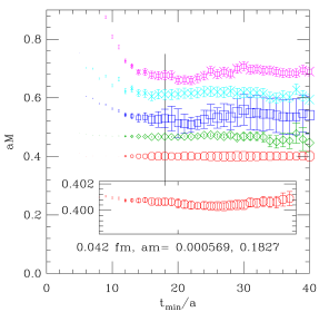
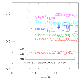
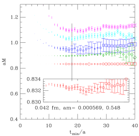
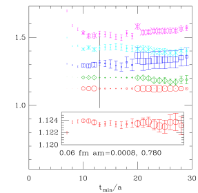
Figure 3: (top) Masses for all 3+2 states in light-charm fits on the $a\approx 0.042$ fm (left) and 0.06 fm (right) physical quark-mass ensembles versus the minimum distance used for the random-wall correlator. (bottom) Same as top panels but for light-heavy fits where the heavy-quark mass is three times the charm quark mass. The vertical and horizontal ranges in all plots are matched in physical units. The vertical lines show the minimum distance in the random wall source correlators used in our analysis. The inserts show the ground-state mass with an expanded vertical scale. The size of the symbol is proportional to the $p$-value of the fit, with a $p$-value of 0.5 corresponding to the size of the label text.

In this plot, the size of the symbols is proportional to the quality of the fit $p$. We compute the $p$ values of our fits using the augmented $\chi^{2}$ that includes both data and prior contributions, and counting the degrees of freedom as the number of data points minus the number of unconstrained fit parameters. Thus it provides a measure of the compatibility of the fit result with both the data and the prior constraints. At small $t_{\text{min}}$ the $p$-value is poor, and more states would be required to get a good fit. At intermediate distances, the masses are mostly determined by the data, while at the largest distances the fit simply returns the prior central values and errors for excited-state and opposite-parity masses. We also perform heavy-light fits using 2+1 states with larger minimum distances as a check, and use the difference between results of the 3+2 state fits and 2+1 state fits to estimate systematic errors coming from excited state contamination. Based on studies like Fig. 3 on every ensemble, we choose the minimum distances $t_{\text{min}}/a$ so that $t_{\text{min}}$ is as close as possible to the minimum distances given in Table 5. As seen in this table, we use a slightly smaller $t_{\text{min}}/a$ for the Coulomb wall source since these correlators have smaller excited state contamination than the random wall source correlators.

We expect the $p$ values to be approximately uniformly distributed, with possible systematic deviations from uniformity coming from artificially loose or tight priors on the mass gaps, and, more importantly, neglecting effects of autocorrelations on the covariance matrix of the correlator at different distances. Figure 4 shows the distribution of $p$ values for our full set of correlator fits using the fit ranges and number of states in Table 5.

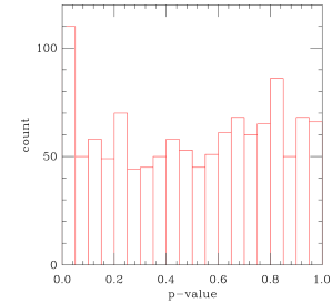
Figure 4: Distribution of $p$ values for our preferred two-point correlator fits in Table 5.

It is approximately uniform from $0$ to $1$, indicating that we have not introduced any systematic bias in our fits from the choice of fit ranges or number of states. Because the $p$-values from correlators with different valence-quark masses in the same ensemble are strongly correlated, the statistical fluctuations in this histogram are larger than the expectation $1/\sqrt{N}$ for independent data.

Table 5: Minimum distances used in our two-point correlator fits. Here “light” quarks include masses up to $m_{s}$ and “heavy” quarks masses beginning at $m_{c}$, and the two numbers in the second column are the number of pseudoscalar and opposite-parity states included in the fit. The “$*$” indicates that this minimum distance is actually taken to depend weakly on the heavy quark mass, with the quoted distance the one used for the $D_{s}$ correlator.

meson	$N_{\text{states}}$	random wall	Coulomb wall
light-light	1+1	2.31 fm	2.11 fm
heavy-light	3+2	0.77 fm	0.68 fm
heavy-light	2+1	1.13∗fm	1.01 fm
heavy-heavy	3+2	0.80 fm	0.68 fm
heavy-heavy	2+1	1.40 fm	1.28 fm

In order to subsequently fit the decay constants and masses obtained from these two-point correlator fits to an EFT function of the quark masses and lattice spacing, we need an estimate of the covariance matrix between these data. (Here the heavy-light decay constant is to be understood as $\Phi$.) To distinguish this covariance matrix from the matrix of covariances of the correlators at different distances used in the two-point fits, in this section we refer to matrices of covariances of masses $M$ and decay constants $\Phi$ as “M$\Phi$ covariance matrices”. In the M$\Phi$ covariance matrix, all of the amplitudes and decay constants for different sets of valence quark masses are correlated, while those from different ensembles are uncorrelated. Thus, the M$\Phi$ covariance matrix is a large block-diagonal matrix, with each block corresponding to a single ensemble.

To obtain each block of the M$\Phi$ covariance matrix, we use a single-elimination jackknife procedure, omitting one configuration at a time from the two-point fits. This approach does not account for autocorrelations. Unfortunately, however, it is not practical to eliminate large enough blocks in the jackknife to suppress the autocorrelations, since we need a number of jackknife blocks that is large compared to the dimension of the block of the M$\Phi$ covariance matrix for that ensemble. We therefore use an approximate procedure. We first compute the block of the M$\Phi$ covariance matrix from the single-elimination jackknife, and then compute the dimensionless correlation matrix by rescaling rows and columns so that the diagonal elements are one. Next we compute the diagonal elements of the M$\Phi$ covariance matrix (that is, the variances of the masses and decay constants) using a block size large enough to reasonably well suppress the effects of autocorrelation, and rescale the rows and columns of the M$\Phi$ covariance matrix to set its diagonal elements equal to the variances obtained from blocking. On all ensembles with $a\gtrsim 0.09$ fm, we blocked the configurations by four; we used larger block sizes of up to 24 configurations on ensembles with finer lattice spacings to account for the longer autocorrelation times. This approach uses the single-elimination jackknife to determine the (dimensionless) correlations of all the masses and decay constants, and the blocked jackknife, which accounts for autocorrelations between gauge-field configurations, to determine the variances of each mass or decay constant.

The M$\Phi$ covariance matrix used in the EFT fit affects the $p$-value of the fit and the central values obtained for the decay constants at the physical quark masses and in the continuum limit. The statistical errors on the masses and decay constants in the M$\Phi$ covariance matrix range from $0.005\%$ to $0.12\%$ and $0.04\%$ to $1.4\%$, respectively. The statistical errors quoted on the physical, continuum-limit decay constants are, however, obtained by an overall jackknife procedure, where we repeat the entire fitting chain 20 times, each time omitting $1/20$ of the configurations from each ensemble.

IV Lattice spacing and quark-mass tuning

Tuning the masses of the light and charm quarks and the determination of the lattice spacings follow the procedure described in detail in Ref. Bazavov et al. (2014a); *Bazavov:2014lja. In this procedure, we use the meson masses and decay constants in the physical quark mass ensembles (with a small correction for mistuned light quark mass), extrapolated to the continuum, to find the $u$, $d$, $s$, and $c$ quark masses used in subsequent steps, and the lattice spacings of each ensemble. For setting the overall scale we use the pion decay constant $f_{\pi}$. We also compute an intermediate scale $f_{p4s}$, the decay constant of a fictitious pseudoscalar meson with degenerate valence quark with mass $m_{p4s}=0.4m_{s}$. To obtain $f_{p4s}$ and the associated meson mass $M_{p4s}$, we draw quadratic functions in the valence-quark mass through the decay-constant and meson-mass data with degenerate valence quarks at 0.3, 0.4 and 0.6 times $m^{\prime}_{s}$, and evaluate these quadratic functions at 0.4 times the tuned strange quark mass $m_{s}$. The quantity $f_{p4s}$ is convenient since it has small statistical errors and can be computed without light valence quark mass correlators. This feature is essential for the $0.03$ fm ensemble where the lightest valence quark mass is $m^{\prime}_{s}/5$, so an extrapolation to $f_{\pi}$ on this ensemble would have large errors.

An initial value for the charm quark mass comes from matching the $D_{s}$ mass. With this $m_{c}$ and the light quark masses, we evaluate the masses of the $D^{0}$ and $D^{+}$ mesons. The difference between them, $2.6$ MeV, can be considered to be the part of the $D^{+}$-$D^{0}$ mass difference coming from the difference in the up and down quark masses. In Sec. VI, this quantity is denoted $C(m_{d}-m_{u})$ and used to estimate the electromagnetic contribution to the mass splitting.

As discussed in Sec. II, the main new aspects of this work are the addition of three new ensembles and the increased statistics on some of the others. We also make some minor updates of the input parameters. The value of $f_{\pi}$, used to set the scale, has been updated to $130.50\pm 0.13$ MeV following the PDG Patrignani et al. (2016); Rosner et al. (2015), and the experimental neutral kaon and charmed meson masses have also seen slight changes.

In contrast with Ref. Bazavov et al. (2014a); *Bazavov:2014lja, we now use the strong coupling $\alpha_{V}$ at scale $q=2.0/a$ obtained from Ref. Chakraborty et al. (2015); *Chakraborty:2017aca in our central fit, and use $\alpha_{T}$, inferred from taste splittings, in an alternative fit to estimate systematic errors.

We also update the quantities $(M^{2}_{K^{0}})^{\gamma}$ and $\epsilon^{\prime}$, which describe electromagnetic effects, to reflect the most recent results from the MILC Collaboration Basak et al. (2014, 2015, 2018). The quantity $(M^{2}_{K^{0}})^{\gamma}$ is the electromagnetic contribution to the squared mass of the neutral kaon. The quantity $\epsilon^{\prime}$ captures higher-order corrections to Dashen’s theorem:

$$\epsilon^{\prime}\equiv\frac{(M^{2}_{K^{\pm}}-M^{2}_{K^{0}})^{\gamma}-(M^{2}_{\pi^{\pm}}-M^{2}_{\pi^{0}})^{\textrm{expt}}}{(M^{2}_{\pi^{\pm}}-M^{2}_{\pi^{0}})^{\textrm{expt}}}.$$ (9)

We use $\epsilon^{\prime}$ rather than the closely related quantity $\epsilon$ defined in Ref. Aoki et al. (2017) as

$$\epsilon\equiv\frac{(M^{2}_{K^{\pm}}-M^{2}_{K^{0}})^{\gamma}-(M^{2}_{\pi^{\pm}}-M^{2}_{\pi^{0}})^{\gamma}}{(M^{2}_{\pi^{\pm}}-M^{2}_{\pi^{0}})^{\textrm{expt}}}.$$ (10)

Because the experimental pion splitting is largely due to electromagnetism, $\epsilon$ and $\epsilon^{\prime}$ are close in size. The difference is estimated in Refs. Gasser and Leutwyler (1985); Aoki et al. (2017) to be

$$\epsilon-\epsilon^{\prime}\equiv\epsilon_{m}=0.04(2),$$ (11)

which is used to find $\epsilon^{\prime}$.

In this paper, we use Basak et al. (2018)

$$\epsilon^{\prime} =0.74(1)_{\rm stat}({}^{+\phantom{1}8}_{-11})_{\rm syst},$$ (12)

$$(M^{2}_{K^{0}})^{\gamma} =44(3)_{\rm stat}(25)_{\rm syst}~{}\text{MeV}^{2}.$$ (13)

Our adjusted kaon masses, or “QCD masses”, are then found from

$$({M_{K^{+}}^{2}})^{\text{QCD}} =M_{K^{+}}^{2}-\left(1+\epsilon^{\prime}\right)\left(M_{\pi^{+}}^{2}-M_{\pi^{0}}^{2}\right)-(M^{2}_{K^{0}})^{\gamma},$$ (14)

$$({M_{K^{0}}^{2}})^{\text{QCD}} =M_{K^{0}}^{2}-(M^{2}_{K^{0}})^{\gamma}.$$ (15)

These quantities are used to match pure QCD to the more fundamental QCD+QED. Consequently, any pure QCD calculation will have uncertainties coming from the particular scheme for separating electromagnetic and isospin effects. Our scheme is the one introduced for $u$ and $d$ quarks in Ref. Borsanyi et al. (2013) and extended naturally to the $s$ quark using the fact that mass renormalization for staggered quarks is multiplicative Basak et al. (2018). As an estimate of the change that would result from the use of a different, but still reasonable, scheme, MILC compares to a scheme where the EM mass renormalization is calculated perturbatively (at one loop). While the resulting scheme dependence of $\epsilon^{\prime}$ is small, $\pm 0.038$ Basak et al. (2018), that of $(M^{2}_{K^{0}})^{\gamma}$ is $\sim 420~{}\text{MeV}^{2}$, much larger than the errors in this quantity in a fixed scheme, although still small compared to $M_{K^{0}}^{2}$.

Table 6 summarizes the experimental masses that we use, and also the “QCD masses” where we have made the adjustments for electromagnetic effects described above, and the adjustments for the heavy meson masses from Eq. (36) in Sec. VI.

Table 6: Experimental inputs to our tuning procedure (left side) Patrignani et al. (2016), and the meson masses after adjusting for electromagnetic effects (right side).

Experimental inputs		QCD masses
$f_{\pi^{+}}$ =	$130.50(1)_{\text{exp.}}(3)_{\text{$V_{ud}$}}(13)_{\text{EM}}$ MeV
$M_{\pi^{0}}$ =	134.9770 MeV	($M_{\pi})^{\text{QCD}}$ =	134.977 MeV
$M_{\pi^{+}}$ =	139.5706 MeV
$M_{K^{0}}$ =	497.611(13) MeV	($M_{K^{0}})^{\text{QCD}}$ =	497.567 MeV
$M_{K^{+}}$ =	493.677(16) MeV	($M_{K^{+}})^{\text{QCD}}$ =	491.405 MeV
$M_{K^{0}}-M_{K^{+}}$ =	3.934(20) MeV
$M_{D_{s}}$ =	1968.28(10) MeV	($M_{D_{s}})^{\text{QCD}}$ =	1967.02 MeV
$M_{B_{s}}$ =	5366.89(19) MeV	($M_{B_{s}})^{\text{QCD}}$ =	5367.11 MeV

We extrapolate the scale-setting quantities $f_{p4s}$ and $M_{p4s}$ and the quark-mass ratios $m_{u}/m_{d}$, $m_{s}/m_{l}$, and $m_{c}/m_{s}$ on the physical quark-mass ensembles to the continuum using a quadratic function in $\alpha_{s}a^{2}$. The fit of $m_{c}/m_{s}$ including all lattice spacings is poor, with $p=0.01$, because discretization errors from the charm quark are large at our coarsest lattice spacing. The $m_{c}/m_{s}$ fit improves substantially to $p=0.8$ when the $a\approx 0.15$ fm data are omitted. In an analysis of the heavy-light-meson masses in Ref. Bazavov et al. (2018), we encounter similar problems when including data from the $a\approx 0.15$ fm ensembles. We therefore omit the $a\approx 0.15$ fm ensembles from our central continuum extrapolations here, in Ref. Bazavov et al. (2018), and in the EFT analysis of the heavy-light decay constants in Sec. V. For estimating systematic errors from our choice of continuum extrapolation of scale-setting quantities, we also consider a fit quadratic in $\alpha_{s}a^{2}$ including all five physical quark-mass ensembles (as was done in Ref. Bazavov et al. (2014a); *Bazavov:2014lja), a fit linear in $\alpha_{s}a^{2}$ omitting the $0.15$ fm ensemble, a fit linear in $\alpha_{s}a^{2}$ omitting both the $0.15$ fm and $0.12$ fm ensembles, and a fit using $\alpha_{s}$ inferred from taste violations.

Figure 5 shows these extrapolations for the intermediate scale $f_{p4s}$.

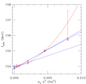
Figure 5: Continuum extrapolations for $f_{p4s}$ on the physical quark mass ensembles. Our central fit, shown in red, is quadratic in $\alpha_{s}a^{2}$ excluding the 0.15 fm data. Alternative fits used for estimating systematic error are shown in blue. These include a quadratic fit including all the data, a linear fit including data up to 0.12 fm, and a linear fit including data up to 0.09 fm. The large error bar on the central fit line shows the statistical error on this fit at $0.15$ fm, the point that is not included in this fit.

In this fit, as in the other quantities discussed in this section, the central fit, shown in red, is at one end of the various extrapolations to $a=0$. We therefore assign a one-sided systematic error from continuum extrapolations equal to the difference between this continuum extrapolation and the furthest of our alternative fits.

We assign five distinct systematic uncertainties to scale-setting quantities and quark-mass ratios stemming from electromagnetic effects, and tabulate them in Table 7.

Table 7: Electromagnetic errors on, and estimates of scheme dependence of scale-setting parameters, quark mass ratios, and, for convenience, the phenomenologically interesting ratio $f_{K^{+}}/f_{\pi^{+}}$, and the ratio of the kaon to pion decay constants in the isospin symmetric limit, $f_{K}/f_{\pi}$.

Error (%)	$f_{p4s}$	$M_{p4s}$	$f_{p4s}/M_{p4s}$	$m_{u}/m_{d}$	$m_{s}/m_{l}$	$m_{c}/m_{s}$	$f_{K^{+}}/f_{\pi^{+}}$	$f_{K}/f_{\pi}$
$K^{+}$-$K^{0}$ splitting	${}_{-0.0033}^{+0.0045}$	${}_{-0.011}^{+0.015}$	${}_{-0.011}^{+0.008}$	${}_{-1.44}^{+1.98}$	${}_{-0.021}^{+0.029}$	${}_{-0.032}^{+0.023}$	${}_{-0.006}^{+0.008}$	${}_{-0.000}^{+0.000}$
$K^{0}$ mass	0.0014	0.006	0.003	0.000	0.011	0.012	0.001	0.007
$H_{x}$ mass	na	na	na	na	na	0.109	na	na
$K$-mass scheme	0.027	0.093	0.065	0.691	0.188	0.205	0.025	0.025
$H_{s}$-mass scheme	na	na	na	na	na	0.365	na	na

The first of these, labeled “$K^{+}$-$K^{0}$ splitting,” is obtained by shifting $\epsilon^{\prime}$ by the lower error bar, $-0.11$, in Eq. (12), and the error in the other direction is obtained by scaling by $-8/11$. Varying the result for $(M^{2}_{K^{0}})^{\gamma}$ in Eq. (13) by its total error gives the second error, labeled “$K^{0}$ mass.” The uncertainty labeled “$K$-mass scheme” is an estimate of the variation that would be produced by matching QCD+QED to pure QCD in an alternative reasonable scheme. This is not taken to be a systematic error in our results, since we work in a fixed, well-defined, scheme. However, when using our results in a setting that does not take into account the subtleties of the EM scheme, one may wish to incorporate the estimate of scheme-dependence as an additional uncertainty. The two remaining electromagnetic uncertainties, which are discussed in more detail in Sec. VI, arise from electromagnetic effects on the relevant heavy-light meson masses. In fact, only the EM effect on the mass of the $D_{s}$, used to fix the charm quark mass, is needed here. From the estimates in Sec. VI, this effect is about 1.3 MeV, which is subtracted from the experimental $D_{s}$ mass before tuning the charm-quark mass, and 100% of the resulting shift is included in our systematic error estimates in the column labeled “$H_{x}$ mass.” Scheme dependence arises again in the EM contribution to the $D_{s}$ mass, and we estimate it at 4.2 MeV in Sec. VI. The resulting uncertainty is listed in the column labeled “$H_{s}$-mass scheme.” The three uncertainties that do not arise from the choice of scheme, namely $K^{+}$-$K^{0}$ splitting, $K^{0}$ mass, and $H_{x}$ mass, are summed in quadrature to give the error labeled “Electromagnetic corrections” in the full error budget, Table 8.

Another systematic error comes from possible incomplete adjustments for the effects of incorrect sampling of the distribution of the topological charge. Using the corrections found in Ref. Bernard and Toussaint (2018) and described in Sec. II.3, we adjust the meson masses and decay constants on the 0.042 and 0.03 fm ensembles to compensate for the incorrect average of the squared topological charge. We conservatively take 100% of the effects of this adjustment as a systematic error coming from poor sampling of the topological charge distribution.

Corrections for finite spatial volume are estimated by the same procedure as in Ref. Bazavov et al. (2014a); *Bazavov:2014lja, where our central fit includes adjustments calculated in NLO staggered chiral perturbation theory, and an associated systematic error is taken to be the difference between this adjustment and using nonstaggered finite-volume chiral perturbation theory, at NNLO for $M_{\pi}$ and $f_{\pi}$, and NLO for $M_{K}$ and $f_{K}$. These estimates are considerably smaller than in Ref. Bazavov et al. (2014a); *Bazavov:2014lja because we have now dropped from the central fit the coarsest ensembles, with $a\approx 0.15$ fm, which dominate the earlier estimate. The taste-splittings at the next coarsest lattice spacing, $a\approx 0.12$ fm, are about a factor of 2 smaller than at $a\approx 0.15$ fm Bazavov et al. (2013), so the difference between staggered and nonstaggered chiral perturbation theory is correspondingly reduced when the $a\approx 0.15$ fm data are dropped.

Finally, we propagate the uncertainty in the PDG value of $f_{\pi}$. The main effect is an overall scale error in dimensionful quantities. Because the decay constants depend on quark masses, an indirect effect also arises, leading to an uncertainty on dimensionless ratios, and a reduction in the uncertainty on dimensionful quantities, compared to the direct scale error. For the ratio $m_{u}/m_{d}$ the experimental uncertainty in $M_{K^{0}}-M_{K^{+}}$ is also included.

Table 8 shows the error budgets for the outputs of the scale-setting and quark-mass-ratio analysis, which are used in the subsequent fitting of the heavy-light results.

Table 8: Error budgets in per cent for scale-setting parameters, quark mass ratios, $f_{K^{+}}/f_{\pi^{+}}$, and $f_{K}/f_{\pi}$.

Error (%)	$f_{p4s}$	$M_{p4s}$	$f_{p4s}/M_{p4s}$	$m_{u}/m_{d}$	$m_{s}/m_{l}$	$m_{c}/m_{s}$	$f_{K^{+}}/f_{\pi^{+}}$	$f_{K}/f_{\pi}$
Statistics	0.072	0.033	0.080	1.20	0.17	0.12	0.13	0.10
Continuum extrapolation	${}_{-0.078}^{+0}$	${}_{-0}^{+0.036}$	${}_{-0.10}^{+0}$	${}_{-0}^{+1.47}$	${}_{-0}^{+0.24}$	${}_{-0.47}^{+0}$	${}_{-0.14}^{+0}$	${}_{-0.12}^{+0}$
Electromagnetic corrections	${}_{-0.004}^{+0.005}$	${}_{-0.012}^{+0.016}$	${}_{-0.011}^{+0.008}$	${}_{-1.45}^{+1.99}$	${}_{-0.024}^{+0.031}$	${}_{-0.115}^{+0.112}$	${}_{-0.007}^{+0.010}$	${}_{-0.003}^{+0.004}$
Topological-charge distribution	0.001	0.000	0.001	0.040	0.061	0.001	0.012	0.012
Finite-volume corrections	0.011	0.001	0.009	0.081	0.059	0.002	0.021	0.016
$f_{\pi,\text{PDG}}$	0.075	0.001	0.075	0.010	0.004	0.051	0.023	0.024
$\Delta M_{K}$	0.000	0.000	0.000	0.283	0.000	0.000	0.001	0.000

The central values for these quantities are listed in Sec. VII.2.

V Effective-field-theory analysis

In this section, we discuss how we combine the lattice data for the meson masses and decay constants described in the previous sections to obtain continuum-limit, physical-quark-mass results. There are two crucial features of our data set. First, as discussed in Sec. II, the range of parameters is broader than that commonly encountered in lattice-QCD calculations. Figure 6 shows the lattice spacings and pion masses of the ensembles used in our analysis.

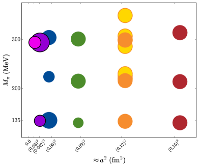
Figure 6: Distribution of four-flavor QCD gauge-field ensembles used in this work. Ensembles that are new with respect our previous analysis Bazavov et al. (2014a); *Bazavov:2014lja are indicated with black outlines. Ensembles with unphysical strange-quark masses are shown as gold disks with orange outlines. The area of each disk is proportional to the statistical sample size $N_{\text{conf}}\times N_{\text{src}}$. The physical, continuum limit is located at $(a=0,M_{\pi}\approx 135~{}\text{MeV})$.

The lattice spacing spans the range $0.03~{}\text{fm}\lesssim a\lesssim 0.15~{}\text{fm}$, while the light sea-quark mass lies between ${\textstyle\frac{1}{2}}(m_{u}+m_{d})\lesssim m^{\prime}_{l}\lesssim 0.2m_{s}$. With the HISQ action, it is possible to simulate physical charm and bottom quarks with controlled discretization errors. Figure 7 shows the range of valence heavy-quark masses used in our analysis. On the coarsest $a\approx 0.15$ and 0.12 fm ensembles, we have only two values $m_{h}=0.9m^{\prime}_{c}$ and $m^{\prime}_{c}$; on our finest $a\approx 0.042$ and 0.03 fm ensembles, however, we have several heavy-quark masses between $0.9m^{\prime}_{c}\leq m_{h}\leq 5m^{\prime}_{c}$, reaching just above the physical $b$-quark mass. Second, as discussed in Sec. III, we have large statistical sample sizes, with about 4,000 samples on most ensembles and large lattice volumes; the resulting errors on the decay constants range from $0.04\%$ to $1.4\%$.

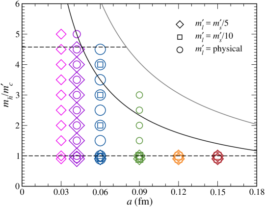
Figure 7: Valence heavy-quark masses vs. lattice-spacings of ensembles used in this calculation, in units of the simulation charm sea-quark mass. Symbol shapes indicate the value of the light sea-quark masses, with diamonds, squares, and circles corresponding to $m^{\prime}_{l}=m^{\prime}_{s}/5$, $m^{\prime}_{s}/10$, and physical, respectively. The symbol area is proportional to the statistical sample size. The black (gray) hyperbola shows $am_{h}=0.9$ ($am_{h}=\pi/2$). The horizontal dashed lines indicate the physical bottom and charm masses.

Because of the breadth and precision of the data set, it is a challenge to find a theoretically well-motivated functional form that is sophisticated enough to describe the whole data set. We therefore rely on several EFTs to parameterize the dependence of our data on each of the independent variables just described: Symanzik effective field theory for lattice spacing dependence Symanzik (1983), chiral perturbation theory for light- and strange-quark mass dependence, and heavy-quark effective theory for the heavy-quark mass dependence. These EFTs are linked together within heavy-meson rooted all-staggered chiral perturbation theory (HMrAS$\chi$PT) Bernard and Komijani (2013). Here we use the one-loop HMrAS$\chi$PT expression to describe the nonanalytic behavior of the interaction between pion (and other pseudo-Goldstone bosons) and the heavy-light meson, and supplement it with higher-order analytic functions in the light- and heavy-quark masses and lattice spacing to enable a good correlated fit.

Even with these additional terms, however, the extrapolation $a\to 0$ and the interpolation $m_{h}\to m_{b}$ oblige us to restrict the range of $am_{h}$. In practice, we are able to obtain a good correlated fit of our data with heavy-quark masses $am_{h}\leq 0.9$. Note, however, that our final fit function describes even the data with $am_{h}>0.9$ quite well.

The rest of this section is organized as follows. In Sec. V.1, we construct an EFT-based fit function with enough parameters (60) to describe the data as a function of the light- and heavy-quark masses and lattice spacing. For convenience, the complete final expression is written out in Sec. V.2. Next, Sec. V.3 explains how we convert our decay-constant data from lattice units to “$p4s$ units” and, eventually, to MeV. Finally, we describe how the fit works in practice and present our final fit used to obtain the decay-constant central values and errors in Sec. V.4.

V.1 Effective-field-theory fit function for heavy-light decay constants

Recall that $H_{x}$ denotes a generic heavy-light pseudoscalar meson composed of a light valence quark $x$ and a heavy valence antiquark $\bar{h}$, with masses $m_{x}$ and $m_{h}$, respectively. The decay constant and mass of $H_{x}$ are $f_{H_{x}}$ and $M_{H_{x}}$, respectively. In heavy-quark physics, the conventional decay constant is defined and normalized as $\Phi_{H_{x}}\equiv f_{H_{x}}\sqrt{M_{H_{x}}}$.

We start with massless light quarks, with $\Phi_{0}$ and $M_{0}$ denoting the decay constant and the meson mass in this limit. We parametrize $\Phi_{0}$ as

$$\Phi_{0}={C\tilde{\Phi}_{0}}\left[1+k_{1}\left(\frac{\Lambda_{\text{HQET}}}{M_{0}}\right)+k_{2}\left(\frac{\Lambda_{\text{HQET}}}{M_{0}}\right)^{2}+\cdots\right],$$ (16)

where $\tilde{\Phi}_{0}$ is the matrix element of the HQET current in the infinite-mass limit, $\Lambda_{\text{HQET}}$ is a physical scale for HQET effects that we set to 800 MeV in this analysis, and the Wilson coefficient $C$ arises from matching the QCD current and the HQET current Ji and Musolf (1991); Manohar and Wise (2000) at scale $m_{h}$:

$$C=\left[\alpha_{s}(m_{h})\right]^{{\gamma_{0}}/{2\beta_{0}}}\left[1+\frac{\alpha_{s}(m_{h})}{4\pi}\left(-\frac{8}{3}+\frac{\gamma_{1}}{2\beta_{0}}-\frac{\gamma_{0}\beta_{1}}{2\beta_{0}^{2}}\right)+\text{O}(\alpha_{s}^{2})\right],$$ (17)

with $\gamma_{0}=-4$, $\gamma_{1}=-254/9-56\pi^{2}/27+20n_{f}/9$, $\beta_{0}=(11-2n_{f}/3)$ and $\beta_{1}=(102-28n_{f}/3)$ with $n_{f}=4$ in our simulations. The Wilson coefficient is usually defined to depend on the renormalization scale $\mu$ of the HQET current, with the renormalization scale (and scheme) dependence canceling between the Wilson coefficient and the HQET matrix element. We have moved this scale dependence out of $C$ into the matrix element $\tilde{\Phi}_{0}$, thereby making $\tilde{\Phi}_{0}$ a renormalization-group invariant quantity. Consequently, $C$ depends only on the matching scale $m_{h}$.

As mentioned in Sec. II, we use $m^{\prime}_{l}$, $m^{\prime}_{s}$, and $m^{\prime}_{c}$ to denote the simulation masses of the light (up-down), strange, and charm quarks, respectively; without the primes $m_{l}={\textstyle\frac{1}{2}}(m_{u}+m_{d})$, $m_{s}$, and $m_{c}$ denote the correctly tuned masses of the corresponding quarks.

We now discuss the dependence of $\Phi_{H_{x}}$ on the deviation of $m^{\prime}_{c}$ from $m_{c}$. The charm quark can be integrated out for processes that occur at energies well below its mass. By decoupling Appelquist and Carazzone (1975), the effect of a heavy (enough) sea quark on low-energy quantities occurs only through the change it produces in the effective value of $\Lambda_{\text{QCD}}$ in the low-energy (three-flavor) theory Bernreuther and Wetzel (1982). We use $\Lambda_{\text{QCD}}^{(3)}(m^{\prime}_{c})$ to denote the effective value of $\Lambda_{\text{QCD}}$ when the charm quark with mass $m^{\prime}_{c}$ is integrated out. At leading order in weak-coupling perturbation theory, one obtains (Manohar and Wise, 2000, Eq. (1.114))

$$\frac{\Lambda_{\text{QCD}}^{(3)}(m^{\prime}_{c})}{\Lambda_{\text{QCD}}^{(3)}(m_{c})}=\left(\frac{m^{\prime}_{c}}{m_{c}}\right)^{2/27}.$$ (18)

Noting that $\tilde{\Phi}_{0}$ has mass-dimension 3/2, we take into account the effects of the mistuned mass $m^{\prime}_{c}$ by assuming $m^{\prime}_{c}\approx m_{c}$ and replacing

$$\tilde{\Phi}_{0}\to\tilde{\Phi}_{0}\left(1+\frac{3}{27}k^{\prime}_{1}\frac{\delta m^{\prime}_{c}}{m^{\prime}_{c}}\right)\left(\frac{m^{\prime}_{c}}{m_{c}}\right)^{3/27},$$ (19)

where $\delta m^{\prime}_{c}=m^{\prime}_{c}-m_{c}$, and $k^{\prime}_{1}$ is a new fit parameter to describe higher-order effects.

Within the framework of HMrAS$\chi$PT Bernard and Komijani (2013), Eq. (16) can be extended to include the light-quark mass dependence and taste-breaking discretization errors of a generic $H_{x}$ meson. This provides a suitable fit function to perform a combined EFT fit to lattice data at multiple lattice spacings and various valence- and sea-quark masses. The fit function that we use in this analysis has the following schematic form

$$\Phi_{H_{x}} =C\tilde{\Phi}_{0}\left[1+k_{1}\frac{\Lambda_{\text{HQET}}}{M_{H_{s}}}+k_{2}\left(\frac{\Lambda_{\text{HQET}}}{M_{H_{s}}}\right)^{2}+k_{3}\left(\frac{\Lambda_{\text{HQET}}}{M_{H_{s}}}\right)^{3}\right]$$

$$\times\left(1+\frac{3}{27}k^{\prime}_{1}\frac{\delta m^{\prime}_{c}}{m^{\prime}_{c}}\right)\left(\frac{m^{\prime}_{c}}{m_{c}}\right)^{3/27}\times\big{(}1+\delta\Phi_{\text{NLO}}+\delta\Phi_{\text{N${}^{n}$LO,analytic}}\big{)},$$ (20)

where $M_{H_{s}}$ is the mass of a pseudoscalar meson with physical sea-quark masses, physical valence strange-quark mass and heavy-quark mass $m_{h}$. In the last parentheses, $\delta\Phi_{\text{NLO}}$ contains the next-to-leading order (NLO) staggered chiral nonanalytic and analytic terms, and $\delta\Phi_{\text{N${}^{n}$LO,analytic}}$ contains higher order analytic terms in the valence and sea-quark masses. For an isospin-symmetric sea with $m_{u}=m_{d}\equiv m_{l}$, we have Bernard and Komijani (2013)

$$\delta\Phi_{\text{NLO}}= -\frac{1}{16\pi^{2}f^{2}}\frac{1}{2}\Biggl{\{}\frac{1}{16}\sum_{\mathscr{S},\Xi}\ell(m_{\mathscr{S}x_{\Xi}}^{2})+\frac{1}{3}\sum_{j\in\mathcal{M}_{I}^{(2,x)}}\frac{\partial}{\partial m^{2}_{X_{I}}}\left[R^{[2,2]}_{j}(\mathcal{M}_{I}^{(2,x)};\mu^{(2)}_{I})\ell(m_{j}^{2})\right]$$

$$\qquad\qquad\quad+\Bigl{(}a^{2}\delta^{\prime}_{V}\sum_{j\in\hat{\mathcal{M}}_{V}^{(3,x)}}\frac{\partial}{\partial m^{2}_{X_{V}}}\left[R^{[3,2]}_{j}(\hat{\mathcal{M}}_{V}^{(3,x)};\mu^{(2)}_{V})\ell(m_{j}^{2})\right]+[V\to A]\Bigr{)}\Biggr{\}}$$

$$-\frac{1}{16\pi^{2}f^{2}}\frac{3g_{\pi}^{2}}{2}\Biggl{\{}\frac{1}{16}\sum_{\mathscr{S},\Xi}J(m_{\mathscr{S}x_{\Xi}},\Delta^{*}+\delta_{\mathscr{S}x})$$

$$\qquad\qquad\quad+\frac{1}{3}\sum_{j\in\mathcal{M}_{I}^{(2,x)}}\frac{\partial}{\partial m^{2}_{X_{I}}}\left[R^{[2,2]}_{j}(\mathcal{M}_{I}^{(2,x)};\mu^{(2)}_{I})J(m_{j},\Delta^{*})\right]$$

$$\qquad\qquad\quad+\Bigl{(}a^{2}\delta^{\prime}_{V}\sum_{j\in\hat{\mathcal{M}}_{V}^{(3,x)}}\frac{\partial}{\partial m^{2}_{X_{V}}}\left[R^{[3,2]}_{j}(\hat{\mathcal{M}}_{V}^{(3,x)};\mu^{(2)}_{V})J(m_{j},\Delta^{*})\right]+[V\to A]\Bigr{)}\Biggr{\}}\$$

$${}+L_{\text{s}}(2x_{l}+x_{s})+L_{x}x_{x}+{\textstyle\frac{1}{2}}L_{a}x_{\bar{\Delta}},$$ (21)

where the indices $\mathscr{S}$ and $\Xi$ run over sea-quark flavors and meson tastes, respectively; $\Delta^{*}$ is the lowest-order hyperfine splitting; $\delta_{\mathscr{S}x}$ is the flavor splitting between a heavy-light meson with light quark of flavor $\mathscr{S}$ and one of flavor $x$; $\delta^{\prime}_{V}$ and $\delta^{\prime}_{A}$ are taste-breaking hairpin parameters; and $g_{\pi}$ is the $H$-$H^{*}$-$\pi$ coupling. Definitions of the residue functions $R_{j}^{[n,k]}$, the sets of masses in the residues, and the chiral functions $\ell$ and $J$ at infinite and finite volumes are given in Ref. Bernard and Komijani (2013) and references therein. At tree-level in HMrAS$\chi$PT, the squared pion mass is linear in the sum of quark masses, $M_{\pi}^{2}\approx B_{0}(m_{u}+m_{d})+a^{2}\Delta_{\Xi}$, where $B_{0}$ is a low-energy constant (LEC) and the splitting $a^{2}\Delta_{P}=0$ for the taste-pseudoscalar pion. We exploit this relation to define dimensionless quark masses and a measure of the taste-symmetry breaking as

$$x_{q} \equiv\frac{2M_{p4s}^{2}}{16\pi^{2}f_{\pi}^{2}}\frac{m_{q}}{m_{p4s}},$$ (22)

$$x_{\bar{\Delta}} \equiv\frac{2}{16\pi^{2}f_{\pi}^{2}}a^{2}\bar{\Delta},$$ (23)

where $q$ denotes the valence or sea light quark and $a^{2}\bar{\Delta}$ is the mean-squared pion taste splitting. The $x_{q}$s and $x_{\bar{\Delta}}$ are natural variables of HMrAS$\chi$PT; the LECs $L_{\text{s}}$, $L_{x}$, and $L_{a}$ are therefore expected to be of order 1. The taste splittings have been determined to $\sim 1$–10% precision Bazavov et al. (2013) and are used as input to Eq. (21).

Because we have very precise data and approximately 500 data points, NLO HMrAS$\chi$PT is not adequate to describe fully the quark-mass dependence, in particular for masses near $m_{s}$. We therefore include all mass-dependent analytic terms at next-to-next-to-leading order (NNLO) and next-to-next-to-next-to-leading order (NNNLO) by defining

$$\delta\Phi_{\text{N${}^{n}$LO,analytic}} =q_{1}x_{x}^{2}+q_{2}(2x_{l}+x_{s})x_{x}+q_{3}(2x_{l}+x_{s})^{2}+q_{4}(2x_{l}^{2}+x_{s}^{2})$$

$$\hphantom{=}+q_{5}x_{x}^{3}+q_{6}(2x_{l}+x_{s})x_{x}^{2}+q_{7}(2x_{l}+x_{s})^{2}x_{x}+q_{8}(2x_{l}^{2}+x_{s}^{2})x_{x}$$

$$\hphantom{=}+q_{9}(2x_{l}+x_{s})^{3}+q_{10}(2x_{l}+x_{s})(2x_{l}^{2}+x_{s}^{2})+q_{11}(2x_{l}^{3}+x_{s}^{3})+q_{12}x_{x}^{4}.$$ (24)

The terms that depend upon the light valence-quark mass are needed to describe our wide range of correlated data with $x_{l}\leq x_{x}\leq x_{s}$. The terms without $x_{x}$ are expected to be less important for obtaining a good fit because most of the ensembles have similar strange sea-quark masses, and because the ensembles are statistically independent, but we include them to make it a systematic approximation at the level of analytic terms. We also include a quartic term $q_{12}x_{x}^{4}$, again to describe our wide range of valence-quark masses.

The staggered chiral form in Eq. (21) is given at fixed heavy-quark mass $m_{h}$, or equivalently at fixed $M_{H_{s}}$. As discussed above, the LECs in Eq. (21) encode the effects of short-distance physics, and the dependence can be parameterized as expansions in inverse powers of the meson mass $M_{H_{s}}$ and powers of the lattice spacing of each ensemble. To take the effects at scale $M_{H_{s}}$ into account, we replace

$$L_{x}\to L_{x}+L^{\prime}_{x}\left(\frac{\Lambda_{\text{HQET}}}{M_{H_{s}}}-\frac{\Lambda_{\text{HQET}}}{M_{D_{s}}}\right)+L^{\prime\prime}_{x}\left(\frac{\Lambda_{\text{HQET}}}{M_{H_{s}}}-\frac{\Lambda_{\text{HQET}}}{M_{D_{s}}}\right)^{2},$$ (25)

and similarly for $L_{\text{s}}$ and $g_{\pi}$. We do not introduce any corrections to $L_{a}$ because it is suppressed by a factor of $\alpha_{s}^{2}a^{2}$ at the finest lattice spacings where the heavy-quark mass dependence could be important. (At coarsest lattice spacings we only have valence heavy-quark masses near charm and thus the variation due to the valence heavy-quark masses is less important.) We also add a $1/M_{H_{s}}$ correction term (but not $1/M^{2}_{H_{s}}$) to the four analytic terms at NNLO:

$$q_{i}\to q_{i}+q^{\prime}_{i}\left(\frac{\Lambda_{\text{HQET}}}{M_{H_{s}}}-\frac{\Lambda_{\text{HQET}}}{M_{D_{s}}}\right),$$ (26)

for $i=1,2,3,4$.

Meson-mass dependence also appears implicitly through the hyperfine splitting $\Delta^{*}$ and the flavor splitting $\delta_{\mathscr{S}x}$ in Eq. (21). To fix the heavy-mass dependence of $\Delta^{*}$, which first appears at order $1/m_{h}$, we use

$$\Delta^{*}=A_{\Delta^{*}}\frac{\Lambda_{\text{HQET}}}{M_{H_{s}}}+B_{\Delta^{*}}\left(\frac{\Lambda_{\text{HQET}}}{M_{H_{s}}}\right)^{2},$$ (27)

with $A_{\Delta^{*}}$ and $B_{\Delta^{*}}$ fixed by demanding that $\Delta^{*}$ reproduce the experimental values of the hyperfine splitting in the $D$ and $B$ systems. Similarly, we determine $\delta_{\mathscr{S}x}$ by writing

$$\delta_{\mathscr{S}x}=A_{\delta}+B_{\delta}\frac{\Lambda_{\text{HQET}}}{M_{H_{s}}},$$ (28)

and fixing $A_{\delta}$ and $B_{\delta}$ from the known flavor splittings in the $D$ and $B$ systems.

To enable a description of our data with a wide range of lattice spacings from $0.03~{}\text{fm}\lesssim a\lesssim 0.15~{}\text{fm}$, we incorporate lattice artifacts into the fit function as follows. Taste-breaking discretization errors in masses of light mesons, which affect the decay constants of heavy-light mesons at one-loop in $\chi$PT, are already included in the staggered chiral form in Eq. (21). In addition to these NLO effects, various discretization errors in the LECs must be taken into account. In Appendix B, we use HQET to study heavy-quark discretization effects at the tree level El-Khadra et al. (1997); Kronfeld (2000). At the leading order, tree-level heavy-quark discretization errors are eliminated via a normalization factor, and at the next order in HQET discretization errors start at order $x_{h}^{4}$ and $\alpha_{s}x_{h}^{2}$, where $x_{h}=2am_{h}/\pi$. For these and generic lattice artifacts, we replace in Eq. (20)

$$\tilde{\Phi}_{0}\to\tilde{\Phi}_{0}\left[1+c_{1}\alpha_{s}(a\Lambda)^{2}+c_{2}(a\Lambda)^{4}+c_{3}(a\Lambda)^{6}+\alpha_{s}\left(c_{4}x_{h}^{2}+c_{5}x_{h}^{4}+c_{6}x_{h}^{6}\right)\right],$$ (29)

where $\Lambda$ is the scale of generic discretization effects, set to 600 MeV in this analysis. A factor of $\alpha_{s}$ is included in the $c_{1}$ and $c_{4}$ terms because the HISQ action is tree-level improved to order $a^{2}$ Naik (1989), so the leading generic discretization errors start at order $\alpha_{s}(a\Lambda)^{2}$ or $\alpha_{s}(am_{h})^{2}$. In addition, a factor of $\alpha_{s}$ is included in the $c_{5}$ and $c_{6}$ terms because of the tree-level normalization factor. For $k_{1}$ and $k_{2}$ in Eq. (20), we likewise replace

$$k_{1} \to k_{1}\left[1+c^{\prime}_{1}\alpha_{s}(a\Lambda)^{2}+c^{\prime}_{2}(a\Lambda)^{4}+c^{\prime}_{3}x_{h}^{4}+\alpha_{s}\left(c^{\prime}_{4}x_{h}^{2}+c^{\prime}_{5}x_{h}^{4}\right)\right],$$ (30)

$$k_{2} \to k_{2}\left[1+c^{\prime\prime}_{1}\alpha_{s}(a\Lambda)^{2}+c^{\prime\prime}_{2}\alpha_{s}x_{h}^{2}\right].$$ (31)

No factor of $\alpha_{s}$ is included in the $c^{\prime}_{3}$ term, because $k_{1}$ parametrizes effects at NLO in HQET.

Let us return to the parameters $L_{x}$, $L_{\text{s}}$, and $g_{\pi}$ found in $\delta\Phi_{\text{NLO}}$. Owing to the Naik improvement term, it is enough to introduce corrections of order $\alpha_{s}(a\Lambda)^{2}$ and $(a\Lambda)^{4}$. Similarly, we add $\alpha_{s}(a\Lambda)^{2}$ corrections to the NNLO analytic terms in Eq. (24). Finally, to incorporate effects of heavy-quark discretization errors, we include

$$\frac{\Lambda_{\text{HQET}}}{M_{H_{s}}}\alpha_{s}x_{h}^{2}$$ (32)

corrections to $L_{x}$, $L_{\text{s}}$, and $g_{\pi}$, as explained in Appendix B.

Our final EFT fit function has 60 fit parameters. With reasonable prior constraints on the large number of parameters describing discretization effects [three parameters at NLO in S$\chi$PT ($\delta^{\prime}_{V}$, $\delta^{\prime}_{A}$, $L_{a}$); 16 parameters for generic discretization effects in powers of $(a\Lambda)$; 10 parameters for the heavy-quark discretization], the uncertainties from the continuum extrapolation are propagated to the statistical error reported by the fit. We test this expectation in Sec. VI by looking at the stability of the results to changes in the widths of the prior constraints, the number of fit parameters, and the data included in the fit.

V.2 Summary formula

In summary, letting $\mathcal{F}$ be our fit function from Sec. V.1, and letting blue (arXiv) denote fit parameters, we have

$$\mathcal{F} =C\breve{\Phi}_{0}\left(1+\breve{k}_{1}w_{h}+\breve{k}_{2}w_{h}^{2}+{{\color[rgb]{0,0,1}{k}_{3}}}w_{h}^{3}\right)\left(1+\frac{3}{27}{{\color[rgb]{0,0,1}k^{\prime}_{1}}}\frac{\delta m^{\prime}_{c}}{m^{\prime}_{c}}\right)\left(\frac{m^{\prime}_{c}}{m_{c}}\right)^{3/27}$$

$$\quad\times\left[1+\delta\Phi_{\text{NLO}}+\sum_{i=1}^{4}\left({{\color[rgb]{0,0,1}q_{i}}}+{{\color[rgb]{0,0,1}q^{\prime}_{i}}}\bar{w}_{h}+{{\color[rgb]{0,0,1}\tilde{q}_{i}}}\alpha_{s}y\right)x_{i}^{2}+\sum_{j=5}^{11}{{\color[rgb]{0,0,1}q_{j}}}x_{j}^{3}+{{\color[rgb]{0,0,1}q_{12}}}x_{x}^{4}\right]$$ (33)

where $y=(a\Lambda)^{2}$, $w_{h}={\Lambda_{\text{HQET}}}/M_{H_{s}}$, $\bar{w}_{h}={\Lambda_{\text{HQET}}}(M_{H_{s}}^{-1}-M_{D_{s}}^{-1})$, and the indices $i$ and $j$ correspond to the labels of the terms in Eq. (24). The chiral logarithm term $\delta\Phi_{\text{NLO}}$ is given by Eq. (21) with the replacements $L_{\text{s}}\to\breve{L}_{\text{s}}$, $L_{x}\to\breve{L}_{x}$, and $g_{\pi}\to\breve{g}_{\pi}$. It depends upon the LECs ${{\color[rgb]{0,0,1}f}}$, ${{\color[rgb]{0,0,1}L_{a}}}$, ${{\color[rgb]{0,0,1}\delta^{\prime}_{V}}}$, and ${{\color[rgb]{0,0,1}\delta^{\prime}_{A}}}$; the hyperfine splitting $\Delta^{*}$; and the taste-independent flavor splitting $\delta_{\mathscr{S}x}$. The breved quantities include terms that allow for the $\chi$PT parameters $\tilde{\Phi}_{0}$, $k_{1}$, $k_{2}$, $L_{x}$, $L_{\text{s}}$, and $g_{\pi}$ to have heavy-quark mass and lattice-spacing dependence:

$$\breve{\Phi}_{0} ={{\color[rgb]{0,0,1}\tilde{\Phi}_{0}}}\left[1+{{\color[rgb]{0,0,1}c_{1}}}\alpha_{s}y+{{\color[rgb]{0,0,1}c_{2}}}y^{2}+{{\color[rgb]{0,0,1}c_{3}}}y^{3}+\alpha_{s}\left({{\color[rgb]{0,0,1}c_{4}}}x_{h}^{2}+{{\color[rgb]{0,0,1}c_{5}}}x_{h}^{4}+{{\color[rgb]{0,0,1}c_{6}}}x_{h}^{6}\right)\right],$$ (34a)

$$\breve{k}_{1} ={{\color[rgb]{0,0,1}k_{1}}}\left[1+{{\color[rgb]{0,0,1}c^{\prime}_{1}}}\alpha_{s}y+{{\color[rgb]{0,0,1}c^{\prime}_{2}}}y^{2}+{{\color[rgb]{0,0,1}c^{\prime}_{3}}}x_{h}^{4}+\alpha_{s}\left({{\color[rgb]{0,0,1}c^{\prime}_{4}}}x_{h}^{2}+{{\color[rgb]{0,0,1}c^{\prime}_{5}}}x_{h}^{4}\right)\right],$$ (34b)

$$\breve{k}_{2} ={{\color[rgb]{0,0,1}k_{2}}}\left(1+{{\color[rgb]{0,0,1}c^{\prime\prime}_{1}}}\alpha_{s}y+{{\color[rgb]{0,0,1}c^{\prime\prime}_{2}}}\alpha_{s}x_{h}^{2}\right),$$ (34c)

$$\breve{L}_{x} ={{\color[rgb]{0,0,1}L_{x}}}+{{\color[rgb]{0,0,1}L^{\prime}_{x}}}\bar{w}_{h}+{{\color[rgb]{0,0,1}L^{\prime\prime}_{x}}}\bar{w}_{h}^{2}+{{\color[rgb]{0,0,1}\tilde{L}^{\prime}_{x}}}\alpha_{s}y+{{\color[rgb]{0,0,1}\tilde{L}^{\prime\prime}_{x}}}y^{2}+{{\color[rgb]{0,0,1}L^{\prime\prime\prime}_{x}}}w_{h}\alpha_{s}x_{h}^{2},$$ (34d)

$$\breve{L}_{\text{s}} ={{\color[rgb]{0,0,1}L_{\text{s}}}}+{{\color[rgb]{0,0,1}L^{\prime}_{\text{s}}}}\bar{w}_{h}+{{\color[rgb]{0,0,1}L^{\prime\prime}_{\text{s}}}}\bar{w}_{h}^{2}+{{\color[rgb]{0,0,1}\tilde{L}^{\prime}_{\text{s}}}}\alpha_{s}y+{{\color[rgb]{0,0,1}\tilde{L}^{\prime\prime}_{\text{s}}}}y^{2}+{{\color[rgb]{0,0,1}L^{\prime\prime\prime}_{\text{s}}}}w_{h}\alpha_{s}x_{h}^{2},$$ (34e)

$$\breve{g}_{\pi} ={{\color[rgb]{0,0,1}g_{\pi}}}+{{\color[rgb]{0,0,1}g^{\prime}_{\pi}}}\bar{w}_{h}+{{\color[rgb]{0,0,1}g^{\prime\prime}_{\pi}}}\bar{w}_{h}^{2}+{{\color[rgb]{0,0,1}\tilde{g}^{\prime}_{\pi}}}\alpha_{s}y+{{\color[rgb]{0,0,1}\tilde{g}^{\prime\prime}_{\pi}}}y^{2}+{{\color[rgb]{0,0,1}g^{\prime\prime\prime}_{\pi}}}w_{h}\alpha_{s}x_{h}^{2}.$$ (34f)

Thus, there are a total of 60 fit parameters. Of these $f$ is constrained by expectations from $\chi$PT, $g_{\pi}$ is constrained by the results of other lattice-QCD calculations, and $\delta^{\prime}_{V}$ and $\delta^{\prime}_{A}$ are constrained by MILC’s light-pseudoscalar-meson $\chi$PT fits.

V.3 Setting the lattice scale for the EFT analysis

We set the lattice scale with a two-step procedure that combines the pion decay constant with the so-called $p4s$ method, in a way similar to Ref. Bazavov et al. (2014a); *Bazavov:2014lja. In the first step of the procedure, we use the PDG value of $f_{\pi}$, $f_{\pi,\text{PDG}}=130.50(13)~{}\text{MeV}$ Patrignani et al. (2016); Rosner et al. (2015), to set the overall scale and to determine tuned quark masses for each physical-mass ensemble. Then, as described in Sec. IV, we calculate $M_{p4s}$ and $f_{p4s}$, which are the mass and decay constant of a pseudoscalar meson with both valence-quark masses equal to $m_{p4s}\equiv 0.4m_{s}$, and with physical sea-quark masses. The continuum-extrapolated values of $f_{p4s}$, $R_{p4s}\equiv f_{p4s}/M_{p4s}$, and quark mass ratios are then used as inputs to the second step of the procedure, which we refer to as the $p4s$ method. In the $p4s$ method, we find $am_{p4s}$ and $af_{p4s}$ on a given physical-mass ensemble by adjusting the valence-quark mass $am_{x}$ until $(af_{x})/(aM_{x})$ takes the same value as the continuum-limit ratio $R_{p4s}$ just determined. In the $p4s$ method, we use a mass-independent scale setting, in which all ensembles at the same $\beta$ as a physical-mass ensemble have, by definition, the same lattice spacing $a=(af_{p4s})/f_{p4s}$ and $am_{p4s}$.

Table 9: Lattice spacing $a$ and $am_{s}$ (in lattice units) in the $p4s$ mass-independent scale-setting scheme. The error associated with $f_{\pi,\text{PDG}}$ is a multiplicative error for all values of $\beta$; the relative error is about $0.15\%$ for lattice spacing $a$ and about $0.3\%$ for $am_{s}$. The uncertainty labeled “EM scheme” is an additional uncertainty that can be incorporated when these results are used without attention to the EM scheme dependence.

$\beta$	$a$ (fm)	$am_{s}$
$5.8\phantom{8}$	$0.15293(26)_{\text{stat}}(19)_{\text{syst}}(23)_{f_{\pi,\text{PDG}}}[07]_{\text{EM scheme}}$	$0.06852(24)_{\text{stat}}(22)_{\text{syst}}(20)_{f_{\pi,\text{PDG}}}[05]_{\text{EM scheme}}$
$6.0\phantom{8}$	$0.12224(16)_{\text{stat}}(15)_{\text{syst}}(18)_{f_{\pi,\text{PDG}}}[05]_{\text{EM scheme}}$	$0.05296(15)_{\text{stat}}(17)_{\text{syst}}(15)_{f_{\pi,\text{PDG}}}[04]_{\text{EM scheme}}$
$6.3\phantom{8}$	$0.08785(17)_{\text{stat}}(11)_{\text{syst}}(13)_{f_{\pi,\text{PDG}}}[04]_{\text{EM scheme}}$	$0.03627(14)_{\text{stat}}(12)_{\text{syst}}(10)_{f_{\pi,\text{PDG}}}[02]_{\text{EM scheme}}$
$6.72$	$0.05662(13)_{\text{stat}}(07)_{\text{syst}}(08)_{f_{\pi,\text{PDG}}}[03]_{\text{EM scheme}}$	$0.02176(10)_{\text{stat}}(07)_{\text{syst}}(06)_{f_{\pi,\text{PDG}}}[01]_{\text{EM scheme}}$
$7.0\phantom{8}$	$0.04259(05)_{\text{stat}}(05)_{\text{syst}}(06)_{f_{\pi,\text{PDG}}}[02]_{\text{EM scheme}}$	$0.01564(04)_{\text{stat}}(05)_{\text{syst}}(04)_{f_{\pi,\text{PDG}}}[01]_{\text{EM scheme}}$
$7.28$	$0.03215(14)_{\text{stat}}(28)_{\text{syst}}(05)_{f_{\pi,\text{PDG}}}[01]_{\text{EM scheme}}$	$0.01129(10)_{\text{stat}}(19)_{\text{syst}}(03)_{f_{\pi,\text{PDG}}}[01]_{\text{EM scheme}}$

To determine $am_{p4s}$ and $af_{p4s}$ accurately, the data must be adjusted for mistunings in the sea-quark masses. To make these adjustments, we use the derivatives with respect to quark masses, which were calculated in our earlier work and listed in Table VII of Ref. Bazavov et al. (2014a); *Bazavov:2014lja. We then iterate, computing $am_{p4s}$ and $af_{p4s}$, readjusting the data, and repeating the entire process until the values of $am_{p4s}$ and $af_{p4s}$ converge within their statistical errors. The results for the lattice spacing $a$ and $am_{s}=2.5am_{p4s}$ are listed in Table 9. For the smallest lattice spacing, $a\approx 0.03$ fm, where we do not have an approximately physical-mass ensemble, we rely on the derivatives to determine $a$ and $am_{s}$ from data on the $m^{\prime}_{l}/m^{\prime}_{s}=0.2$ ensemble, leading to larger relative systematic errors at $\beta=7.28$.

V.4 Effective-field-theory fit to heavy-light decay constants

In Sec. V.1, we have constructed an EFT fit function that contains 60 fit parameters. We use this function to perform a combined, correlated fit to the partially-quenched data at the five lattice spacings, from $a\approx 0.12$ fm to $\approx 0.03$ fm, and at several values of the light sea-quark masses. The sixth lattice spacing, $a\approx 0.15$ fm, is used in a check of the estimate of discretization errors, but not included in the base fit used to obtain our central values and statistical errors. At the coarsest lattice spacings, we have data with only two different values for the valence heavy-quark mass: $m_{h}=m^{\prime}_{c}$ and $m_{h}=0.9m^{\prime}_{c}$. Recall that $m^{\prime}_{c}$ is the simulation value of sea charm-quark mass of the ensembles, and is itself not precisely equal to the physical charm mass $m_{c}$ because of tuning errors. At the finest lattice spacings, we have a wide range of valence heavy-quark masses from near charm to bottom. We include all data with $0.9m^{\prime}_{c}\leq m_{h}\leq 5m^{\prime}_{c}$, subject to condition $am_{h}<0.9$, which is chosen to avoid large lattice artifacts. Note that our analysis includes an $a\approx 0.03$ fm, $m^{\prime}_{l}/m^{\prime}_{s}=0.2$, ensemble for which $am_{b}\approx 0.6$, and thus no extrapolation from lighter heavy-quark masses is needed, although a chiral extrapolation to physical light-quark masses is required.

We use a constrained fitting procedure Lepage et al. (2002) with priors set as follows. For the LEC $g_{\pi}$ of the $D$ system, we use the prior $g_{\pi}=0.53\pm 0.08$, which is based on lattice-QCD calculations Bečirević and Sanfilippo (2013); Can et al. (2013); Detmold et al. (2012). For $1/f^{2}$ in Eq. (21), our prior is

$$\frac{1}{f^{2}}=\frac{1}{2}\left(\frac{1}{f_{\pi}^{2}}+\frac{1}{f_{K}^{2}}\right)\pm\left(\frac{1}{f_{\pi}^{2}}-\frac{1}{f_{K}^{2}}\right),$$ (35)

where we set $f_{\pi}=130.5$ MeV and $f_{K}=156$ MeV. For the taste-breaking hairpin parameters, we use priors of $\delta^{\prime}_{A}/\bar{\Delta}=-0.88\pm 0.09$ and $\delta^{\prime}_{V}/\bar{\Delta}=0.46\pm 0.23$, which are taken from chiral fits to light pseudoscalar mesons Bazavov et al. (2011); *Bazavov:2011fh-update. The fits of Ref. Bazavov et al. (2011) have been performed at $a\approx 0.12$ fm, where ensembles with unphysical strange quark masses are available (see Table 1). We take advantage of the fact that both the taste splittings and the hairpin parameters scale like $\alpha^{2}_{s}a^{2}$ at NLO in the chiral expansion, so their ratio remains constant as $a$ changes. For $\tilde{\Phi}_{0}$, we use an extremely wide prior of $0\pm 1000$ in $p4s$ units. The rest of the fit parameters are normalized to be of order 1, and for them we choose a prior of $0\pm 1.5$. We discuss this choice in Sec. VI and argue that it is conservative. Finally, for $\alpha_{s}$ we use the coupling $\alpha_{V}$ at scale $q=2.0/a$, obtained from Ref. Chakraborty et al. (2015); *Chakraborty:2017aca.

Altogether we have $492$ lattice data points in the base fit and $60$ parameters in the EFT fit function. The fit has a correlated $\chi^{2}_{\text{{data}}}/\text{dof}=466/432$, giving $p=0.12$. Figure 8 shows a snapshot of the decay constants for physical-mass ensembles, plotted versus the corresponding heavy-strange meson masses $M_{H_{s}}$ at three lattice spacings.

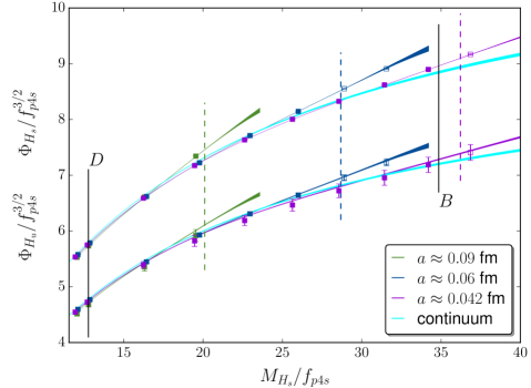
Figure 8: Decay constants plotted in units of $f_{p4s}$ vs the heavy-strange meson mass for physical-mass ensembles at three lattice spacings, and continuum extrapolation. For each color there are two sets of data and fit lines: one with valence light mass $m_{x}=m_{s}$ (higher one), and one with $m_{x}=m_{u}$. The dashed vertical lines indicate the cut $am_{h}=0.9$ for each lattice spacing, and data points (with open symbols) to the right of the dashed vertical line of the corresponding color are omitted from the fit. The width of the fit lines shows the statistical error coming from the fit. The solid vertical lines indicate the $D$ and $B$ systems, where $M_{H_{s}}=M_{D_{s}}$ and $M_{H_{s}}=M_{B_{s}}$, respectively.

The continuum extrapolation is also shown. The valence light mass $m_{x}$ is tuned either to $m_{s}$ (upper points) or to $m_{u}$ (lower points). Data points with open symbols that are at the right of the dashed vertical line of the corresponding color are omitted from the fit because they have $am_{h}>0.9$. The fact that the fit lines agree well with the omitted points is evidence that we have not overfit the data. In the continuum extrapolation, the masses of sea quarks are set to the correctly-tuned, physical quark masses $m_{l}$, $m_{s}$, and $m_{c}$, while at nonzero lattice spacing the masses of the sea quarks take the simulated values.

The width of the fit lines in Fig. 8 shows the statistical error coming from the fit, which is only part of the total statistical error, since it does not include the statistical errors in the inputs of the quark masses and the lattice scale. To determine the total statistical error of each output quantity, we divide the full data set into 20 jackknife resamples. The complete calculation, including the determination of the inputs, is performed on each resample, and the error is computed as usual from the variations over the resamples. (For convenience, we kept the covariance matrix fixed to that from the full data set, rather than recomputing it for each resample.) The same procedure is performed to find the total statistical error of $a$ and $am_{s}$ at each lattice spacing.

The fit function Eq. (20), evaluated at $a=0$ and physical sea-quark masses, yields a parameterization of the decay-constant data as a function of the heavy-strange meson mass $M_{H_{s}}$ and the valence light-quark mass $m_{x}$. We ignore isospin violation in the sea, taking the light sea-quark masses to be degenerate with the average $u/d$-quark mass. Because the HMrAS$\chi$PT expression for the heavy-light meson decay amplitude is symmetric under the interchange $m_{u}\leftrightarrow m_{d}$, the leading contributions from isospin-breaking in the sea sector are of $\text{O}((m_{d}-m_{u})^{2})$, and are expected to be smaller than the NNLO terms in the chiral expansion. We can check numerically the effect of sea isospin-breaking using our data by evaluating the fit function with physical up and down sea-quark masses. The resulting shifts in the decay constants are less than about 0.02% for the $B$ system and 0.015% for the $D$ system, which are consistent with power-counting expectations and are negligible compared to other uncertainties. We obtain the physical charged and neutral $B$- and $D$-meson decay constants by setting $m_{x}$ to either $m_{u}$, $m_{d}$ or $m_{s}$, and $M_{H_{s}}$ to the experimental values $M_{B_{s}}=5366.82(22)$ MeV and $M_{D_{s}}=1968.27(10)$ MeV Patrignani et al. (2016), respectively, along with a prescription to subtract electromagnetic effects from the masses, as discussed below.

VI Systematic error budgets

Figure 9 shows the stability of our final results for $f_{D^{+}}$, $f_{D_{s}}$, $f_{B^{+}}$ and $f_{B_{s}}$ under variations in the data set and the fit models.

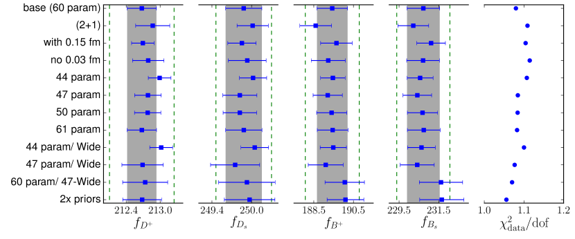
Figure 9: Stability plot showing the sensitivity to different choices of lattice data and fit models. (See the text for description.) The error bars show only the statistical errors, the gray error bands correspond to the statistical error of the base fit, and the green dashed lines correspond to total errors.

In our base fit, we use the decay constants obtained from the (3+2)-state fit to two-point correlators. To investigate the error arising from excited-state contamination, we perform a fit to the decay-constant data obtained from the (2+1)-state fit to two-point correlators. There is some evidence for such contamination, contributing a systematic error that is comparable to the statistical errors for the $B$ system. We take the difference between the results from the two types of correlator fits as an estimate of the systematic error due to excited states. For consistency, we do so both for the $D$ system as well as the $B$ system, even though there is little evidence for such contamination for the $D$ system. It is reasonable that the $B$ correlators suffer from larger excited state effects, because, as seen in Fig. 3, the fits to correlators with heavier quarks tend to have smaller $p$ values at fixed $T_{\text{min}}$, as well as larger errors in the ground state mass.

Figure 9 also shows a test of the systematic error in the continuum extrapolation from repeating the fit after either adding in the coarsest ($a\approx 0.15$ fm) ensembles or omitting the finest ($a\approx 0.03$ fm) ensemble. The differences with the base fit are well within the statistical errors, providing support for our earlier assertion that the continuum-extrapolation errors are already included in our estimate of the statistical uncertainty of our fit.

In our base fit, constrained Bayesian curve fitting Lepage et al. (2002) is employed to incorporate systematic errors in the continuum extrapolation. If the prior values have been chosen in a reasonable way, and if we have sufficiently many parameters in the fit, central values and error bars of final quantities should not change when more parameters are included in the fit. The error bars are then expected to capture the systematic errors in the continuum extrapolation.

To test the priors chosen for discretization effects, we repeat the analysis with different numbers of discretization parameters. The result of this test is shown in Fig. 9. The base fit has 60 parameters. We show results from alternative fits with 44, 47, 50, and 61 parameters. The fit with 50 parameters is constructed from our base EFT fit function by removing 10 terms that describe higher-order discretization effects in powers of $(a\Lambda)^{2}$: specifically, the $(a\Lambda)^{6}$ correction to $\tilde{\Phi}_{0}$; the $(a\Lambda)^{4}$ corrections to $k_{1}$, $L_{\text{s}}$, $L_{x}$ and $g_{\pi}$; and the $(a\Lambda)^{2}$ corrections to $k_{2}$ and the NNLO analytic terms in Eq. (24). In the fit with 47 parameters, three additional terms describing higher-order heavy-quark discretization effects are removed: we set to zero $c^{\prime}_{3}$, $c^{\prime}_{5}$ and $c^{\prime\prime}_{2}$ in Eqs. (30) and (31). The fit with 44 parameters is then obtained by removing, from the 47-parameter fit, the $\alpha_{s}(a\Lambda)^{2}$ corrections to $L_{\text{s}}$, $L_{x}$ and $g_{\pi}$. Finally, we consider a fit function with 61 parameters, which is constructed from our base EFT fit function by adding a term $\alpha_{s}x_{h}^{8}$ to Eq. (29), which is the most important term at the next order in our expansion variables.

The 44-parameter fit shows a significant deviation from the base fit for $f_{D^{+}}$, but already with 47 parameters the deviations of all quantities are small: the errors are essentially unchanged from those of the base fit, and the central values change by no more than half the error bars. Differences between the base fit and the 61-parameter fit are not visible at all. In the context of constrained Bayesian curve fitting Lepage et al. (2002), these findings suggests that the posterior uncertainty captures most or all of the systematic error of the continuum extrapolation.

The priors may be further tested by monitoring the posteriors in various fits. Figure 10 (left) shows the distribution of posterior central values for essentially unconstrained fit parameters (priors $0\pm 100$) in the 44-parameter fit.

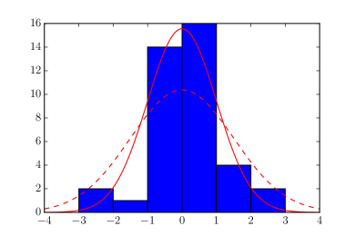
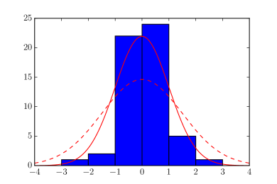
Figure 10: Left: distribution of fit posteriors in a fit with 44 parameters and essentially no prior constraints (prior widths of 100). Right: distribution of fit posteriors in the base fit for parameters constrained with priors $0\pm 1.5$. In each plot the solid and dashed red curves show Gaussian distributions with width 1 and 1.5, respectively.

The distribution is compared to Gaussian distributions with widths of 1 and 1.5. Note that the width-1 Gaussian is already fairly consistent with the distribution, but there may be some indication of excess in the tails. On the other hand, the width-1.5 Gaussian clearly encompasses the posterior distribution. Thus the natural size of these parameters is indeed of order unity, and a prior of $0\pm 1.5$ seems to be a conservative assumption for any additional parameters in other fits that are not well constrained by data. Figure 10 (right) shows the corresponding distribution of posterior central values for the 55 parameters in the base fit that are constrained with priors $0\pm 1.5$. The comparison with the width-1.5 Gaussian indicates that the parameters are not being unnaturally constrained by the Bayesian priors.

In the Bayesian approach, prior information about fit parameters is explicitly put into the fit. A non-Bayesian alternative is to limit the number of fit parameters to those constrained by the data with no external information about what sizes of the parameters are expected. External information nevertheless enters implicitly by assuming that the parameters omitted from the fit are all exactly zero. We apply this alternative approach to test whether there are additional systematic errors in the continuum extrapolation due to the choice of fit function that are not captured by the Bayesian analysis. Figure 9 shows two fits with fewer parameters than the base fit, which may then be determined by the data, with essentially no Bayesian constraint. The fits are labeled “44 param/ Wide” and “47 param/ Wide.” They have the same parameter sets as the 44-parameter and 47-parameter fits discussed above, but now with very wide priors, $0\pm 100$. (The 44 param/ Wide fit yields Figure 10 (left).) We also include a fit, “60 param/ 47-Wide” with the same parameters as the base fit, but with the 47 parameters that can be determined by the data alone now essentially unconstrained by priors and priors of $0\pm 1$ for the remaining 13 parameters. These three new fits have $p$ values larger than 0.05, so we consider them to be acceptable alternatives. Comparing these fits with the base fit, we find that the central values vary a bit more than we would expect from the Bayesian analysis. In particular, $f_{D^{+}}$ in the 44-param/ Wide fit and $f_{B_{s}}$ in the 60 param/ 47-Wide fit differ from the base fit by slightly more than the error bar of the base fit (indicated by the gray band). We take a conservative approach and take the largest of these differences for each quantity as an additional systematic error due to the choice of fit model.

A final fit in Fig. 9, labeled “$2\times$ priors,” starts with the base fit and doubles, to $0\pm 3$, the prior widths of the 55 parameters constrained by power counting arguments. The results of this fit are very similar to those from the 60 param/ 47-Wide fit. In the Bayesian context, it is to be expected that weakening the prior information in the base fit results in an increase in the resulting errors. However, the shifts in the central values for the $B$ system are large enough that the inclusion of the fit model error discussed in the previous paragraph seems prudent.

Tables 10 and 11 give representative error budgets for the decay constants and their ratios in the $D$ and $B$ systems, respectively. The error listed as “statistics and EFT fit” is determined by a jackknife procedure (described at the end of Sec. V.4) in which we repeat, on data resamples, the EFT fit and its extrapolation to the continuum and interpolation to physical quark masses. It includes statistical errors in the inputs as well as those from the fit itself. As explained above, it also includes much of the systematic error associated with the continuum extrapolation. The small errors from the chiral interpolation are likewise captured by our Bayesian procedure, which includes all analytic chiral terms at NNLO and NNNLO.

Table 10: Representative error budgets for decay constants of the $D$ system, estimated as described in the text. Error budgets for $f_{D^{0}}$ and the isospin-limit value $f_{D}$ are similar to that for $f_{D^{+}}$ with one exception. The uncertainty from the topological-charge correction is larger for lighter valence-quark masses: 0.09% (0.07%) for $f_{D^{0}}$ ($f_{D}$).

Error (%)	x$f_{D^{+}}$x	x$f_{D_{s}}$x	x$f_{D_{s}}/f_{D^{+}}$x
Statistics and EFT fit	$0.12$	$0.11$	$0.05$
Two-point correlator fits	$0.09$	$0.05$	$0.04$
Fit model	$0.16$	$0.07$	$0.09$
Scale-setting quantities and tuned quark masses	$0.08$	$0.04$	$0.05$
Finite-volume corrections	$0.02$	$0.01$	$0.01$
Electromagnetic corrections	$0.01$	$0.01$	$0.01$
Topological charge distribution	$0.05$	$0.00$	$0.05$
$f_{\pi,\text{PDG}}$	$0.11$	$0.08$	$0.03$

Table 11: Representative error budgets for decay constants of the $B$ system, estimated as described in the text. Error budgets for $f_{B^{+}}$ and the isospin-limit value $f_{B}$ are similar to that for $f_{B^{0}}$ with one exception. The uncertainty from the topological-charge correction is larger for lighter valence-quark masses: 0.11% (0.08%) for $f_{B^{+}}$ ($f_{B}$).

Error (%)	x$f_{B^{0}}$x	x$f_{B_{s}}$x	x$f_{B_{s}}/f_{B^{0}}$x
Statistics and EFT fit	$0.39$	$0.36$	$0.24$
Two-point correlator fits	$0.39$	$0.22$	$0.17$
Fit model	$0.34$	$0.39$	$0.08$
Scale-setting quantities and tuned quark masses	$0.10$	$0.06$	$0.05$
Finite-volume corrections	$0.03$	$0.01$	$0.02$
Electromagnetic corrections	$0.02$	$0.02$	$0.01$
Topological charge distribution	$0.07$	$0.00$	$0.07$
$f_{\pi,\text{PDG}}$	$0.14$	$0.11$	$0.04$

The error labeled “two-point correlator fits” in Tables 10 and 11 is an estimate of the contamination due to excited states. It is determined by comparison of the results from the base, (3+2)-state, fits and those from (2+1)-state fits.

The error we associate with the choice of fitting function, is labeled “Fit model” in each table. As explained above, it comes from comparing the results of different non-Bayesian (essentially unconstrained) fits to those from the base fit. While the differences are not so large that they necessarily invalidate the Bayesian error analysis, they are large enough that we are inclined to be conservative and include them as a separate source of error. Since the fit model controls the continuum extrapolation, this error may be interpreted as an estimate of those continuum extrapolation errors not completely captured by our Bayesian analysis.

The fourth line in each table, labeled “scale-setting quantities and tuned quark masses,” gives the systematic error associated with the continuum extrapolations of $f_{p4s}$, $R_{p4s}$, and the tuned quark masses. As described in Sec. IV, the central values of these input quantities to the heavy-light analysis come from a quadratic fit in $\alpha_{{s}}a^{2}$ to the ensembles with $a\leq 0.12$ fm. We repeat the heavy-light analysis with the inputs instead determined by three alternatives: a quadratic fit including all the data, a linear fit including data up to 0.12 fm, and a linear fit including data up to 0.09 fm. The errors shown in Tables 10 and 11 are obtained by taking the largest difference between the base values and the results from each of the three alternatives.

The error labeled “finite-volume corrections” gives our estimate of residual finite volume errors, those finite volume effects not included in our chiral fitting forms. The errors associated with light-quark and scale-setting inputs are estimated in the same way as those associated with continuum extrapolation errors of those quantities, using the input finite-volume errors from Table 8. To determine the corresponding finite-volume errors arising directly in the heavy-light analysis, we omit the finite-volume corrections at NLO in $\chi$PT from the EFT fits, and then repeat the fits. We take 0.3 of the differences between the results of the two fits as estimates of the residual finite-volume errors coming from omitted higher-order terms in $\chi$PT. We consider the factor 0.3 to be conservative because higher order corrections in SU(3) $\chi$PT are typically less than that; for example, $f_{K}/f_{\pi}-1\approx 0.2$. We then add the finite volume errors from the heavy-quark analysis in quadrature with those from the inputs to get the values shown in Tables 10 and 11. This is reasonable because we do not know the correlations between the effects of finite volume errors on the light-light and heavy-light quantities. For example, the ratios between heavy-light and light-light decay constants, which enter through our scale-setting procedure, are likely to be less-dependent on volume than either decay constant alone. In any case, if we instead assumed 100% correlation between the light-light and heavy-light finite volume errors, it would make little difference in the total systematic error.

We note that the finite-volume errors in Table 8 are considerably smaller than in earlier drafts of this paper. The previous version was inconsistent, in that it took the input estimate of light-quark finite volume errors from a comparison of fits including the data at $a\approx 0.15$ fm, while our central fit drops that lattice spacing. As discussed in Sec. IV, keeping the $a\approx 0.15$ fm data gives an overestimate of finite-volume effects due to staggered taste splittings that predominantly affect that lattice spacing.

Despite the fact that the decay constants are by definition pure QCD matrix elements of the axial current, there are electromagnetic uncertainties in the values that the meson masses (used primarily to fix the physical quark masses) would have in a pure QCD world. The estimated systematic error labeled “electromagnetic corrections” in Tables 10 and 11 accounts for the two sources of this uncertainty. First, there are electromagnetic errors in the tuned values we use for the light-quark masses that arise from errors in the determinations of the electromagnetic contributions to pion and kaon masses. These correspond to the “$K^{+}$-$K^{0}$ splitting” and “$K^{0}$ mass,” and errors described in Sec. IV. We vary the values of the tuned light-quark masses by these two EM uncertainties in Table 7 to obtain the corresponding uncertainties on the decay constants in Table 12. In this work, we choose a specific scheme Borsanyi et al. (2013); Basak et al. (2018) for the electromagnetic contribution to the neutral kaon masses; other works, for example the FLAG report Aoki et al. (2017), choose other schemes. Changing the scheme so that $\left(M_{K^{0}}^{2}\right)^{\gamma}$ goes from $+44~{}\text{MeV}^{2}$ to $+461~{}\text{MeV}^{2}$ changes the listed quantities by the percentages in row “$K$-mass scheme.”

There are also electromagnetic effects in the heavy-light meson masses, which affect our calculation both directly, in the meson-mass value we use to convert from a $\Phi$ value to a decay constant $f=\Phi/\sqrt{M}$, and indirectly, through the tuned values of the heavy-quark masses. To estimate the resulting electromagnetic errors on the decay constants, we first need to relate the experimental values of the heavy-light meson masses to QCD-only values. For this, we use the phenomenological formula Davies et al. (2010); Goity and Jayalath (2007); Rosner and Wise (1993)

$$M^{\text{expt}}_{H_{x}}=M^{\text{QCD}}_{H_{l}}+Ae_{x}e_{h}+Be_{x}^{2}\,+\,C(m_{x}-m_{l})\,,$$ (36)

where $e_{x}$ and $e_{h}$ are charges of the valence light and heavy quarks, respectively, and we have added a term proportional to $(m_{x}-m_{l})$ to account for the mass difference between $u$ and $d$ quarks. Physical contributions proportional to $e_{h}^{2}$, which come from effects such as the EM correction to the heavy quark’s chromomagnetic moment, are suppressed by $1/m_{h}$, and are therefore dropped from this simple model. There are also prescription (scheme) dependent EM contributions to the heavy quark mass renormalization, which are proportional to $e_{h}^{2}m_{h}$; our choice of scheme is to drop them entirely. To estimate the parameters $A$ and $B$, we use the experimental $D^{0}$-, $D^{+}$-, $B^{+}$- and $B^{0}$–meson masses in Eq. (36), which gives

$$M^{\text{expt}}_{D^{+}}-M^{\text{expt}}_{D^{0}} =+4.75~{}\text{MeV}=\frac{2}{3}A-\frac{1}{3}B+C(m_{d}-m_{u}),$$ (37)

$$M^{\text{expt}}_{B^{+}}-M^{\text{expt}}_{B^{0}} =-0.31~{}\text{MeV}=\frac{1}{3}A+\frac{1}{3}B-C(m_{d}-m_{u}).$$ (38)

Taking $C(m_{d}-m_{u})=2.6$ MeV as described in Sec. IV, we then obtain $A=4.44$ MeV and $B=2.4$ MeV.

Table 12: Error contributions to, and estimates of scheme dependence of, the decay constants from electromagnetic effects. The sources of uncertainty are described in the text.

Error (%)	x$f_{D^{0}}$x	x$f_{D^{+}}$x	x$f_{D_{s}}$x	x$f_{B^{+}}$x	x$f_{B^{0}}$x	x$f_{B_{s}}$x
$K^{+}$-$K^{0}$ splitting	$0.02$	$0.00$	$0.01$	$0.02$	$0.00$	$0.01$
$K^{0}$ mass	$0.00$	$0.00$	$0.00$	$0.00$	$0.00$	$0.00$
$H_{x}$ mass	$0.05$	$0.01$	$0.01$	$0.04$	$0.02$	$0.02$
$K$-mass scheme	$0.03$	$0.03$	$0.05$	$0.04$	$0.03$	$0.06$
$H_{s}$-mass scheme	$0.07$	$0.07$	$0.07$	$0.05$	$0.05$	$0.04$

Using Eq. (36), we estimate that the electromagnetic contribution to the $D_{s}$-meson mass to be about 1.3 MeV, which is substantially smaller than the result, $5.5(6)$ MeV, found for this shift in Ref. Giusti et al. (2017). We emphasize that we do not add any terms in Eq. (36) proportional to $e_{h}^{2}m_{h}$. Such terms, which can explain the difference between results of Ref. Giusti et al. (2017) and Eq. (36), can be absorbed into the heavy-quark mass and do not contribute to electromagnetic mass splittings for the heavy-light mesons. Consequently, these terms only affect the tuned heavy-quark masses, which inevitably depend on the scheme used for matching a pure QCD calculation onto real-world measurements, which include electromagnetism.

We take the difference between results obtained with and without the electromagnetic shift from Eq. (36) as an estimate of the uncertainty in applying our phenomenological model. This error includes effects of neglecting mass-dependent corrections to the parameters $A$ and $B$. We tabulate this error in the row labeled “$H_{x}$ mass.” We also estimate the effect of the scheme dependence of the heavy quark mass, which we call “$H_{s}$-mass scheme,” by taking the difference between the electromagnetic contributions to the $D_{s}$ meson mass obtained from Eq. (36) and the scheme of Ref. Giusti et al. (2017), which includes the heavy-quark self-energy. We do not have corresponding information for the $B_{s}$ meson, so we take the $D_{s}$ shift and simply assume that it is dominated by a mass renormalization term proportional to $e_{h}^{2}m_{h}$. Because $m_{c}e_{c}^{2}\approx m_{b}e_{b}^{2}$, this leads to the same shift, 4.2 MeV, for both $D_{s}$ and $B_{s}$.

The individual electromagnetic EM uncertainties on the decay constants discussed above are tabulated in Table 12. Because we have no information about correlations between the various EM errors, we add the $K^{+}$-$K^{0}$ splitting, $K^{0}$ mass, and $H_{x}$ mass error in quadrature to obtain the total “electromagnetic corrections” entries given in Tables 10 and 11. Even if there were strong correlations between the EM errors, this would make little difference to the total systematic errors of the heavy-light decay constants, because these errors are subdominant, as can be seen in Tables 10 and 11.

The error labeled “topological-charge distribution” accounts for the nonequilibration of topological charge in our finest ensembles. Before our EFT fit, we adjust the lattice data to compensate for effects of nonequilibration of topological charge as discussed in Sec. II.3. We conservatively estimate the uncertainty in our treatment of effects of nonequilibration of topological charge by taking the full difference between the final results of the analyses with and without adjustments.

The last “$f_{\pi,\text{PDG}}$” error included in Tables 10 and 11 is the uncertainty due to the error in the PDG average for the charged-pion decay constant, $f_{\pi^{\pm}}=130.50(13)$ MeV Rosner et al. (2015), which is the physical scale that is used to determine $f_{p4s}$.

All errors in Tables 10 and 11 should be added in quadrature to obtain the total uncertainties. In the following section, when we quote our final results for the physical decay constants, we separate the errors into “statistical” errors, which are the ones listed as “statistics and EFT fit,” “systematic” errors, which are those due to the systematics of our calculation (rows 2–6 in the tables, added in quadrature), and, finally, the errors due to the PDG value of $f_{\pi}$, which is external to our calculation.

As a byproduct of our EFT analysis, we can also obtain the decay amplitudes $\Phi$ for the $D$ and $B$ systems in both the SU(2) and the SU(3) limits, which are reported in Table 13.

Table 13: Results for $\Phi$ in the SU(2) and the SU(3) chiral limits. Here $m_{x}=m^{\prime}_{l}=0$ and the strange sea mass is either $m^{\prime}_{s}=m_{s}$ (in the SU(2) case) or $m^{\prime}_{s}=0$ (in the SU(3) case). The uncertainty labeled “EM scheme” is an additional uncertainty that can be incorporated when these results are used without attention to the EM scheme dependence.

$D$ system	$\Phi_{0}^{\text{SU(3)}}=8133(67)_{\text{stat}}(93)_{\text{syst}}(12)_{f_{\pi,\text{PDG}}}[15]_{\text{EM scheme}}~{}\text{MeV}^{3/2}$
	$\Phi_{0}^{\text{SU(2)}}=8976(12)_{\text{stat}}(24)_{\text{syst}}(11)_{f_{\pi,\text{PDG}}}[17]_{\text{EM scheme}}~{}\text{MeV}^{3/2}$
$B$ system	$\Phi_{0}^{\text{SU(3)}}=11717(205)_{\text{stat}}(181)_{\text{syst}}(21)_{f_{\pi,\text{PDG}}}[11]_{\text{EM scheme}}~{}\text{MeV}^{3/2}$
	$\Phi_{0}^{\text{SU(2)}}=13461(57)_{\text{stat}}(73)_{\text{syst}}(20)_{f_{\pi,\text{PDG}}}[13]_{\text{EM scheme}}~{}\text{MeV}^{3/2}$

VII Results and phenomenological impact

We now present our final results for the heavy-light meson decay constants with total errors and then discuss some of their phenomenological implications.

VII.1 $B$- and $D$-meson decay constants

Our final results for the physical leptonic decay constants of the $D$ and $B$ systems including all sources of systematic uncertainty discussed in the previous section are

$$f_{D^{0}} =211.6(0.3)_{\text{stat}}(0.5)_{\text{syst}}(0.2)_{f_{\pi,\text{PDG}}}[0.2]_{\text{EM scheme}}~{}\text{MeV},$$ (39)

$$f_{D^{+}} =212.7(0.3)_{\text{stat}}(0.4)_{\text{syst}}(0.2)_{f_{\pi,\text{PDG}}}[0.2]_{\text{EM scheme}}~{}\text{MeV},$$ (40)

$$f_{D_{s}} =249.9(0.3)_{\text{stat}}(0.2)_{\text{syst}}(0.2)_{f_{\pi,\text{PDG}}}[0.2]_{\text{EM scheme}}~{}\text{MeV},$$ (41)

$$f_{B^{+}} =189.4(0.8)_{\text{stat}}(1.1)_{\text{syst}}(0.3)_{f_{\pi,\text{PDG}}}[0.1]_{\text{EM scheme}}~{}\text{MeV},$$ (42)

$$f_{B^{0}} =190.5(0.8)_{\text{stat}}(1.0)_{\text{syst}}(0.3)_{f_{\pi,\text{PDG}}}[0.1]_{\text{EM scheme}}~{}\text{MeV},$$ (43)

$$f_{B_{s}} =230.7(0.8)_{\text{stat}}(1.0)_{\text{syst}}(0.2)_{f_{\pi,\text{PDG}}}[0.2]_{\text{EM scheme}}~{}\text{MeV}.$$ (44)

These results are obtained in a specific scheme for matching QCD+QED to pure QCD via the light and heavy meson masses tabulated in Table 6. When using our results in a setting that does not take into account the subtleties of the EM scheme, one may wish to also include the last quantities, in brackets, which are obtained by adding in quadrature the fourth and fifth rows in Table 12, as rough estimates of scheme dependence.

Most recent lattice-QCD calculations of heavy-light meson decay constants work, however, in the isospin-symmetric limit. To enable comparison with these results, we also present results for the $B$- and $D$-meson decay constants evaluated with the light valence-quark mass fixed to the average $u/d$-quark mass:

$$f_{D} =212.1(0.3)_{\text{stat}}(0.4)_{\text{syst}}(0.2)_{f_{\pi,\text{PDG}}}[0.2]_{\text{EM scheme}}~{}\text{MeV},$$ (45)

$$f_{B} =190.0(0.8)_{\text{stat}}(1.0)_{\text{syst}}(0.3)_{f_{\pi,\text{PDG}}}[0.1]_{\text{EM scheme}}~{}\text{MeV}.$$ (46)

Figures 11 and 12 compare our decay-constant results with previous three- and four-flavor lattice-QCD calculations Davies et al. (2010); McNeile et al. (2012); Bazavov et al. (2012); Na et al. (2012a, b); Dowdall et al. (2013a); Christ et al. (2015); Bazavov et al. (2014a); Yang et al. (2015); Carrasco et al. (2015a); Bussone et al. (2016); Boyle et al. (2017); Hughes et al. (2018). They agree with the lattice-QCD averages from the Particle Data Group Rosner et al. (2015):

$$f_{D^{+},\text{\,PDG}} =211.9(1.1)~{}\text{MeV},$$ (47)

$$f_{D_{s},\text{\,PDG}} =249.0(1.2)~{}\text{MeV},$$ (48)

$$f_{B^{+},\text{\,PDG}} =187.1(4.2)~{}\text{MeV},$$ (49)

$$f_{B^{0},\text{\,PDG}} =190.9(4.1)~{}\text{MeV},$$ (50)

$$f_{B_{s},\text{\,PDG}} =227.2(3.4)~{}\text{MeV},$$ (51)

where we note that the $D_{(s)}$ averages are dominated by our earlier result in Ref. Bazavov et al. (2014a); *Bazavov:2014lja.

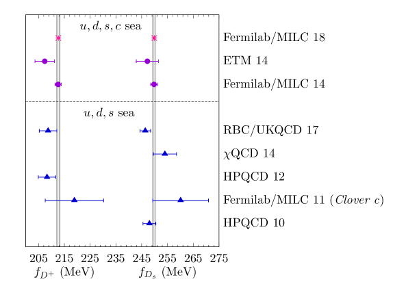
Figure 11: Comparison of our $D$-meson decay-constant results (magenta bursts) with previous three- and four-flavor lattice-QCD calculations Davies et al. (2010); Bazavov et al. (2012); Na et al. (2012b); Bazavov et al. (2014a); Yang et al. (2015); Carrasco et al. (2015a); Boyle et al. (2017). The vertical gray bands show the total uncertainties from Eqs. (40) and (41). The asymmetric errors on the RBC/UKQCD 17 results have been symmetrized.

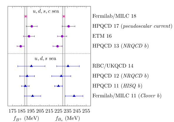
Figure 12: Comparison of $B$-meson decay-constant results (magenta bursts) with previous three- and four-flavor lattice-QCD calculations McNeile et al. (2012); Bazavov et al. (2012); Na et al. (2012a); Dowdall et al. (2013a); Christ et al. (2015); Bussone et al. (2016); Hughes et al. (2018). The vertical gray bands show the total uncertainties from Eqs. (42) and (44).

For the $D$-meson decay constants, the uncertainties in Eqs. (40)–(41) are about 2.5 times smaller than from our previous analysis. The improvement stems primarily from the inclusion of finer ensembles with $a\approx 0.042$ fm and 0.03 fm, which reduce the distance of the continuum extrapolation.

For $B$-meson decay constants, the uncertainties in Eqs. (42)–(44) are approximately three times smaller than from the previous best calculations from HPQCD McNeile et al. (2012); Dowdall et al. (2013a). For $f_{B_{s}}$, HPQCD’s most precise determination was obtained with the HISQ action for $b$ quarks McNeile et al. (2012). The substantial improvement in our result comes from a combination of higher statistics and the ensemble with $a\approx 0.03$ fm, which eliminates the need to extrapolate to the bottom-quark mass from lighter quark masses, and also shortens the continuum extrapolation. For $f_{B^{+}}$ and $f_{B^{0}}$, HPQCD has employed only NRQCD $b$ quarks Dowdall et al. (2013a). Thus, our results for these quantities are the first obtained with the HISQ action for the $b$ quarks. With HISQ, the dominant errors in HPQCD’s calculation—from operator matching and relativistic corrections to the current—simply do not arise.

Because the statistical and several systematic errors are correlated between the decay constants in Eqs (40)–(44), we can obtain combinations of decay constants with even greater precision. Our results for the decay-constant ratios are

$$f_{D_{s}}/f_{D^{+}} =1.1749(06)_{\text{stat}}(14)_{\text{syst}}(04)_{f_{\pi,\text{PDG}}}[03]_{\text{EM scheme}},$$ (52)

$$f_{B_{s}}/f_{B^{+}} =1.2180(33)_{\text{stat}}(33)_{\text{syst}}(05)_{f_{\pi,\text{PDG}}}[03]_{\text{EM scheme}},$$ (53)

$$f_{B_{s}}/f_{B^{0}} =1.2109(29)_{\text{stat}}(25)_{\text{syst}}(04)_{f_{\pi,\text{PDG}}}[03]_{\text{EM scheme}},$$ (54)

$$f_{B_{s}}/f_{D_{s}} =0.9233(25)_{\text{stat}}(42)_{\text{syst}}(02)_{f_{\pi,\text{PDG}}}[03]_{\text{EM scheme}}.$$ (55)

The light quarks in the $D^{+}$ and $D_{s}$ mesons have identical charges, so the deviation of $f_{D_{s}}/f_{D^{+}}$ from unity quantifies the degree of $SU(3)$-flavor breaking in the $D$ system. Similarly, the ratio $f_{B_{s}}/f_{B_{0}}$ characterizes the size of $SU(3)$-breaking in the $B$-meson system. Both yield values of about 20%, which is consistent with power-counting expectations of $(m_{s}-m_{d})/\Lambda_{\text{QCD}}$.

For the differences due to strong isospin breaking (i.e., $m_{u}\neq m_{d}$) we find

$$f_{D^{+}}-f_{D} =0.58(01)_{\text{stat}}(07)_{\text{syst}}(00)_{f_{\pi,\text{PDG}}}[01]_{\text{EM scheme}}~{}\text{MeV},$$ (56)

$$f_{D^{+}}-f_{D^{0}} =1.11(03)_{\text{stat}}(15)_{\text{syst}}(00)_{f_{\pi,\text{PDG}}}[01]_{\text{EM scheme}}~{}\text{MeV},$$ (57)

$$f_{B}-f_{B^{+}} =0.53(05)_{\text{stat}}(07)_{\text{syst}}(00)_{f_{\pi,\text{PDG}}}[00]_{\text{EM scheme}}~{}\text{MeV},$$ (58)

$$f_{B^{0}}-f_{B^{+}} =1.11(08)_{\text{stat}}(13)_{\text{syst}}(00)_{f_{\pi,\text{PDG}}}[01]_{\text{EM scheme}}~{}\text{MeV}.$$ (59)

These results can be employed to correct other lattice-QCD results obtained in the isospin limit, which will be essential once other calculations reach sub-percent precision. For $f_{D^{+}}$, the isospin-breaking correction is larger than our total uncertainty in Eq. (40), while for $f_{B^{+}}$ it is comparable to the total error in Eq. (42). We find a smaller isospin correction to the $B$-meson decay constant than obtained by HPQCD in Ref. Dowdall et al. (2013a), $(f_{B}-f_{B^{+}})_{\text{HPQCD}}=1.9(5)$ MeV, by more than $2\sigma$. HPQCD’s estimate was obtained, however, by setting both the valence- and sea-quark masses in $f_{B^{+}}$ to $m_{u}$ because the analysis only included unitary data. Hence their value includes effects both from valence isospin breaking and from reducing the average light sea-quark mass; when we follow this prescription, we obtain a similarly-large shift of about $1.6(2)$ MeV. On the other hand, our results for the isospin corrections to both $f_{D}$ and $f_{B}$ agree with calculations using Borelized sum rules Lucha et al. (2017, 2018).

Tables 15 and 16 in Appendix C provide the correlation and covariance matrices, respectively, between the $B$- and $D$-meson decay constants in Eqs. (39)–(46). They can be used to compute any combination of our results with the correct uncertainties.

VII.2 Quark-mass ratios, $f_{K}/f_{\pi}$, and scale-setting quantities

In Sec. IV, we analyze the ensembles with physical light-quark masses to obtain several input parameters for the EFT fit of heavy-light meson decay constants. We obtain for the mass and decay constant of a fictitious pseudoscalar-meson with degenerate valence-quark masses $0.4m_{s}$:

$$f_{p4s} =153.98(11)_{\text{stat}}({}_{-12}^{\,+2})_{\text{syst}}(12)_{f_{\pi,\text{PDG}}}[4]_{\text{EM scheme}}~{}\text{MeV},$$ (60)

$$M_{p4s} =433.12(14)_{\text{stat}}({}_{-6}^{+17})_{\text{syst}}(4)_{f_{\pi,\text{PDG}}}[40]_{\text{EM scheme}}~{}\text{MeV},$$ (61)

$$f_{p4s}/M_{p4s} =0.3555(3)_{\text{stat}}({}_{-4}^{+1})_{\text{syst}}(3)_{f_{\pi,\text{PDG}}}[2]_{\text{EM scheme}},$$ (62)

where the last quantity, in brackets, is an additional uncertainty when these results are used without attention to EM scheme dependence. These quantities are used to set the scale in our analysis.

We obtain for the ratios of quark masses:

$$m_{u}/m_{d} =0.4556(55)_{\text{stat}}({}_{-67}^{+114})_{\text{syst}}(13)_{\Delta M_{K}}[32]_{\text{EM scheme}},$$ (63)

$$m_{s}/m_{l} =27.178(47)_{\text{stat}}({}_{-26}^{+70})_{\text{syst}}(1)_{f_{\pi,\text{PDG}}}[51]_{\text{EM scheme}},$$ (64)

$$m_{c}/m_{s} =11.773(14)_{\text{stat}}({}_{-57}^{+14})_{\text{syst}}(6)_{f_{\pi,\text{PDG}}}[49]_{\text{EM scheme}},$$ (65)

where $m_{l}$ is the average $u/d$-quark mass. The errors on the quark-mass ratios in Eqs. (63)–(65) are smaller than from our previous analysis in Ref. Bazavov et al. (2014a); *Bazavov:2014lja because the finer lattice spacings employed here reduce the continuum-extrapolation error. Figures 13 and 14 compare our results for $m_{u}/m_{d}$ and $m_{s}/m_{l}$, respectively, with previous unquenched lattice-QCD calculations. The difference in our value for $m_{s}/m_{l}$ relative to Ref. Bazavov et al. (2014a); *Bazavov:2014lja mostly comes from three changes, which all push the value in the same direction. In order of size, these are the addition of the 0.042 fm physical-quark-mass ensemble, removing the 0.15 fm ensembles from our central fits, and adding more data on the 0.06 fm physical-quark-mass ensembles. An even more precise value for $m_{c}/m_{s}$ is reported in a companion paper on the determination of quark masses from heavy-light meson masses Bazavov et al. (2018).

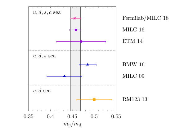
Figure 13: Comparison of $m_{u}/m_{d}$ in Eq. (63) (magenta burst) with previous unquenched lattice-QCD calculations Bazavov et al. (2009); de Divitiis et al. (2013); Carrasco et al. (2014); Basak et al. (2016); Fodor et al. (2016).

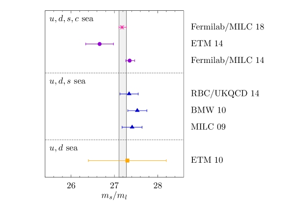
Figure 14: Comparison of $m_{s}/m_{l}$ in Eq. (64) (magenta burst) with previous unquenched lattice-QCD calculations Bazavov et al. (2014a); *Bazavov:2014lja; Bazavov et al. (2009); Baron et al. (2010); Dürr et al. (2011); Carrasco et al. (2014); Blum et al. (2016).

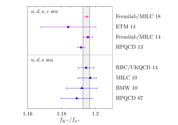
Figure 15: Comparison of $f_{K^{+}}/f_{\pi^{+}}$ in Eq. (66) (magenta burst) with previous three- and four-flavor lattice-QCD calculations Bazavov et al. (2014a); *Bazavov:2014lja; Follana et al. (2008); Dürr et al. (2010); Bazavov et al. (2010b); Dowdall et al. (2013b); Blum et al. (2016); Carrasco et al. (2015a).

Finally, we obtain the ratio of charged pion to kaon decay constants. We also give the ratio in the isospin symmetric limit, and the difference between the two:

$$f_{K^{+}}/f_{\pi^{+}} =1.1950(15)_{\text{stat}}({}_{-17}^{\,+4})_{\text{syst}}(3)_{f_{\pi,\text{PDG}}}[3]_{\text{EM scheme}},$$ (66)

$$f_{\bar{K}}/f_{\pi} =1.1980(12)_{\text{stat}}({}_{-14}^{\,+3})_{\text{syst}}(3)_{f_{\pi,\text{PDG}}}[3]_{\text{EM scheme}},$$ (67)

$$f_{\bar{K}}/f_{\pi}-f_{K^{+}}/f_{\pi^{+}} =0.00305(50)_{\text{stat}}({}_{-12}^{\,+31})_{\text{syst}}(2)_{f_{\pi,\text{PDG}},\Delta M_{K}}[3]_{\text{EM scheme}},$$ (68)

which are again more precise than our previous determination in Ref. Bazavov et al. (2014a); *Bazavov:2014lja because of the shorter continuum extrapolation. Our results agree with previous three- and four-flavor lattice-QCD calculations (see Fig. 15), and with the 2016 FLAG averages Aoki et al. (2017).

VII.3 CKM matrix elements

We now combine our decay-constant results with experimental measurements of the $D^{+}_{(s)}$-meson leptonic decay rates to obtain values for the CKM matrix elements $|V_{cd}|$ and $|V_{cs}|$ within the Standard Model.

The products of decay constants times CKM factors from the Particle Data Group Rosner et al. (2015),

$$\left(f_{D^{+}}|V_{cd}|\right)_{\text{expt}} =45.91(1.05)~{}\text{MeV},$$ (69)

$$\left(f_{D_{s}^{+}}|V_{cs}|\right)_{\text{expt}} =250.9(4.0)~{}\text{MeV},$$ (70)

are obtained by averaging the experimentally-measured decay rates into muon and tau final states. The value for $f_{D^{+}}|V_{cd}|$ in Eq. (69) includes the correction from structure-dependent bremsstrahlung effects that lowers the $D^{+}\to\mu^{+}\nu_{\mu}$ rate by $\sim 1\%$ Burdman et al. (1995); Dobrescu and Kronfeld (2008). Other electroweak corrections, however, are not accounted for in the PDG averages shown above. The electroweak contributions to leptonic pion and kaon decays are estimated to be about one or two percent Cirigliano and Rosell (2007); Cirigliano et al. (2012), and the uncertainties in these corrections lead to $\sim 0.1\%$ uncertainties in $|V_{us}|/|V_{ud}|$ and $|V_{us}|$. Now that the errors on $f_{D}$ and $f_{D_{s}}$ are well below half a percent, electroweak corrections must also be included when extracting $|V_{cd}|$ and $|V_{cs}|$ from leptonic $D$-meson decays.

We take the estimate of the electroweak corrections to the leptonic $D^{+}_{(s)}$-meson decay rates from our earlier work Bazavov et al. (2014a); *Bazavov:2014lja, which includes all contributions that are included for pion and kaon decays. We first adjust the experimental decay rates quoted in the PDG by the known long- and short-distance electroweak corrections Kinoshita (1959); Sirlin (1982). The former lowers the $D^{+}$- and $D_{s}$-meson leptonic decay rates by about 2.5%, while the latter increases them by about $1.8\%$, such that the net effect is a slight decrease in the rates by less than a percent. We then include a 0.6% uncertainty to account for unknown electromagnetic corrections that depend upon the mesons’ structure. This estimate is based on calculations of the structure-dependent electromagnetic corrections to pion and kaon decays Knecht et al. (2000); Cirigliano and Rosell (2007); Descotes-Genon and Moussallam (2005), but allowing for much larger coefficients than for the light pseudoscalar mesons.

With these assumptions, and taking our $D^{+}$- and $D_{s}$-meson decay-constant results from Eqs. (40) and (41), we obtain for the CKM matrix elements

$$|V_{cd}|^{\text{SM},\,f_{D}} =0.2151(6)_{f_{D}}(49)_{\rm expt}(6)_{\rm EM},$$ (71)

$$|V_{cs}|_{\text{SM},\,f_{D_{s}}} =1.000(2)_{f_{D_{s}}}(16)_{\rm expt}(3)_{\rm EM},$$ (72)

where “EM” denotes the error due to unknown structure-dependent electromagnetic corrections. In both cases, the lattice-QCD uncertainties from the decay constants are an order of magnitude smaller than those from experiment. Further, the electromagnetic errors are only a rough estimate, and need to be put on a more robust and quantitative footing by a direct calculation of the hadronic structure-dependent effects.

The CKM matrix elements $|V_{cd}|$ and $|V_{cs}|$ can also be obtained from semileptonic $D^{+}\to\pi^{0}\ell^{+}\nu$ and $D^{+}\to K^{0}\ell^{+}\nu$ decays. Recently the ETM Collaboration published the first four-flavor lattice-QCD determination of the vector and scalar form factors for these processes Lubicz et al. (2017). Combining their form factors over the full range of momentum transfer with experimental measurements of the decay rates yields for the CKM elements Riggio et al. (2018)

$$|V_{cd}|_{D\to\pi} =0.2341(74),$$ (73)

$$|V_{cs}|_{D\to K} =0.970(33),$$ (74)

where the errors are primarily from the theoretical uncertainties on the form factors. Although our result for $|V_{cs}|$ in Eq. (72) agrees with this determination, our result for $|V_{cd}|$ in Eq. (71) is about 2.1$\sigma$ lower than the above value from semileptonic decays. We note, however, that combining $f_{+}^{D\pi}(0)|V_{cd}|=0.1425(19)$ from the Heavy Flavor Averaging Group Amhis et al. (2017a) with $f_{+}^{D\pi}(0)=0.666(29)$ from the most precise three-flavor lattice-QCD calculations by HPQCD Na et al. (2011) leads to a lower value of $|V_{cd}|_{D\to\pi}=0.2140(97)$ that agrees with our result.

Our results for $|V_{cd}|$ and $|V_{cs}|$ make possible a test of the unitarity of the second row of the CKM matrix. Taking $|V_{cb}|_{\text{incl+excl}}=41.40(77)\times 10^{-3}$ from a weighted average of determinations from inclusive and exclusive semileptonic $B$ decays Bailey et al. (2014, 2015a); Na et al. (2015); Gambino et al. (2016); Bigi and Gambino (2016); Bigi et al. (2017), we obtain for the sum of squares of the CKM elements

$$|V_{cd}|^{2}+|V_{cs}|^{2}+|V_{cb}|^{2}-1.0=0.049(2)_{|V_{cd}|}(32)_{|V_{cs}|}(0)_{|V_{cb}|},$$ (75)

which is compatible with three-generation CKM unitarity within 1.5$\sigma$. The precision on the above test is only at the few-percent level, and is limited by the experimental error on the leptonic decay widths for $D_{s}\to\mu\nu_{\mu}$ and $D_{s}\to\tau\nu_{\tau}$.

We can also update the determination of the ratio of CKM elements $|V_{us}/V_{ud}|$ from leptonic pion and kaon decays. Combining our result for $f_{K^{+}}/f_{\pi^{+}}$ in Eq. (66) with the experimental rates and estimated radiative-correction factor from the Particle Data Group Rosner et al. (2015), we obtain

$$|V_{us}/V_{ud}|_{\text{SM}}=0.2310(4)_{f_{K}/f_{\pi}}(2)_{\text{expt}}(2)_{\text{EM}},$$ (76)

where we have averaged the upper and lower errors from our decay-constant ratio.

VII.4 Branching ratios for $B_{q}\to\mu^{+}\mu^{-}$

The rare leptonic decays $B^{0}\to\mu^{+}\mu^{-}$ and $B_{s}\to\mu^{+}\mu^{-}$ proceed via flavor-changing-neutral-current interactions and are therefore promising new-physics search channels. In the $B_{s}$-meson system, the difference between decay widths of the light and heavy mass eigenstates is large, $\Delta\Gamma_{s}/\Gamma_{s}\sim 0.1$ Amhis et al. (2017a), and leads to a difference between the CP-averaged and time-averaged branching ratios. Because only the heavy $B_{s}$ eigenstate can decay to $\mu^{+}\mu^{-}$ pairs in the Standard Model, to a very good approximation Bobeth et al. (2014), the two quantities are related simply as $\overline{\mathcal{B}}(B_{s}\to\mu^{+}\mu^{-})_{\text{SM}}=\tau_{H_{s}}\Gamma(B_{s}\to\mu^{+}\mu^{-})_{\text{SM}}$, where $\tau_{H_{s}}$ is the lifetime of the heavy mass eigenstate, and the bar denotes time averaging. The relative width difference $\Delta\Gamma_{d}/\Gamma_{d}\sim 0.001$ is 100 times smaller in the $B^{0}$-meson system, so $\overline{\mathcal{B}}(B_{s}\to\mu^{+}\mu^{-})=\mathcal{B}(B_{s}\to\mu^{+}\mu^{-})$.

The LHCb and CMS experiments reported the first observation of $B_{s}\to\mu^{+}\mu^{-}$ decay in 2014 Khachatryan et al. (2015). This observation was subsequently confirmed by the ATLAS experiment Aaboud et al. (2016), and LHCb has since improved upon their initial measurement using a larger data set Aaij et al. (2017a). The most recent results for the $B_{s}\to\mu^{+}\mu^{-}$ time-integrated branching fraction are marginally compatible:

$$10^{9}\times\overline{\mathcal{B}}(B_{s}\to\mu^{+}\mu^{-})_{\text{ATLAS}} =0.9(^{+1.1}_{-0.8}),$$ (77)

$$10^{9}\times\overline{\mathcal{B}}(B_{s}\to\mu^{+}\mu^{-})_{\text{LHCb 17}} =3.0(0.6)(^{+0.3}_{-0.2}),$$ (78)

with the LHCb measurement being about $1.8\sigma$ larger. The LHCb and CMS experiments also reported 3$\sigma$ evidence for the decay $B^{0}\to\mu^{+}\mu^{-}$, which is suppressed in the Standard Model relative to $B_{s}\to\mu^{+}\mu^{-}$ by the CKM factor $|V_{td}/V_{ts}|^{2}\sim 0.04$. The significance, however, has subsequently weakened, and ATLAS and LHCb most recently only presented upper limits of Aaboud et al. (2016); Aaij et al. (2017a)

$$\overline{\mathcal{B}}(B^{0}\to\mu^{+}\mu^{-})_{\text{ATLAS}} <3.4\times 10^{-10},$$ (79)

$$\overline{\mathcal{B}}(B^{0}\to\mu^{+}\mu^{-})_{\text{LHCb 17}} <4.2\times 10^{-10},$$ (80)

at 95% confidence level.

Here we update the theoretical predictions for the Standard-Model branching ratios using our results for the neutral $B^{0}$- and $B_{s}$-meson decay constants. We employ the formulae in Eqs. (6) and (7) of Ref. Bobeth et al. (2014), which provide the branching ratios in terms of the decay constants, relevant CKM elements, and a few other parametric inputs. Using the CKM elements and other inputs listed in Table 14, and $f_{B^{0}}$, $f_{B_{s}}$, and their ratio from Eqs. (43)–(44) and (54), we obtain

$$\overline{\mathcal{B}}(B_{s}\to\mu^{+}\mu^{-})_{\text{SM}} =3.64(4)_{f_{B_{s}}}(8)_{\text{CKM}}(7)_{\text{other}}\times 10^{-9},$$ (81)

$$\overline{\mathcal{B}}(B^{0}\to\mu^{+}\mu^{-})_{\text{SM}} =1.00(1)_{f_{B^{0}}}(2)_{\text{CKM}}(2)_{\text{other}}\times 10^{-10},$$ (82)

$$\left(\frac{\overline{\mathcal{B}}(B^{0}\to\mu^{+}\mu^{-})}{\overline{\mathcal{B}}(B_{s}\to\mu^{+}\mu^{-})}\right)_{\text{SM}} =0.0273(2)_{f_{B_{q}}}(5)_{\text{CKM}}(7)_{\text{other}},$$ (83)

where the errors are from the decay constants, CKM matrix elements, and the quadrature sum of all other contributions, respectively. Because $\overline{\mathcal{B}}(B_{q}\to\mu^{+}\mu^{-})$ is proportional to the square of the decay constant, our three-fold improvement in the uncertainty on the $B$-meson decay constants reduces the error contributions from the decay constants by almost a factor of two, such that they are now well below the other sources of uncertainty.

Table 14: Numerical inputs used to calculate $B_{q}\to\mu^{+}\mu^{-}$ branching ratios. The strong coupling (in the $\overline{\rm MS}$ scheme) is a weighted average of three- and four-flavor lattice-QCD results Aoki et al. (2009); McNeile et al. (2010); Blossier et al. (2014); Bazavov et al. (2014c); Chakraborty et al. (2015); Bruno et al. (2017). The $B$-meson lifetimes are from the Heavy Flavor Averaging Group’s Summer 2017 averages Amhis et al. (2017a, b). The CKM matrix elements are from the CKMfitter group’s global unitarity-triangle analysis including results through ICHEP 2016 Charles et al. (2005), where we have symmetrized the errors on $|V_{ts}^{*}V_{tb}|$ and $|V_{td}^{*}V_{tb}|$, and used the Wolfenstein parameters $\left\{\lambda=0.22510(28),A=0.8341(20),\bar{\rho}=0.1600(74),\bar{\eta}=0.3500(62)\right\}$ rather than the simple ratio to obtain $|V_{td}/V_{ts}|$ with a reduced uncertainty.

$m_{t,{\text{pole}}}=173.1(6)~{}\text{GeV}$ Patrignani et al. (2016)	$\alpha_{s}(m_{Z})=0.1186(4)$
$\tau_{B_{d}}={1.518(4)}\;\text{ps}$	$\tau_{H_{s}}={1.619(9)}\;\text{ps}$
$|V_{ts}^{*}V_{tb}|=40.9(4)\times 10^{-3}$	$|V_{td}^{*}V_{tb}|=8.56(9)\times 10^{-3}$
$|V_{td}/V_{ts}|=0.2085(18)$

VIII Summary and outlook

In this paper, we have presented the most precise lattice-QCD calculations to-date of the leptonic decay constants of heavy-light pseudoscalar mesons with charm and bottom quarks. We use highly improved staggered quarks with finer lattice spacings than ever before, which enables us for the first time to work with the HISQ action directly at the physical $b$-quark mass. As shown in Figs. 11 and 12, our results agree with previous three- and four-flavor lattice-QCD determinations using different actions for the light, charm, and bottom quarks. The errors on our $D$-meson decay constants in Eqs. (39)–(41) are about 2.5 times smaller than those from our earlier analysis Bazavov et al. (2014a); *Bazavov:2014lja. The error reduction is primarily due to the use of finer lattice spacings, which reduces the continuum-extrapolation uncertainty. Our $B$-meson decay constants in Eqs. (42)–(44) are about three times more precise than the previous best lattice-QCD calculations by HPQCD McNeile et al. (2012); Dowdall et al. (2013a). Here the improvement again stems from the use of finer lattice spacings, which enable us to employ the HISQ action directly at the physical $m_{b}$ with controlled heavy-quark discretization errors, thereby eliminating the need to extrapolate to the bottom-quark mass from lighter heavy valence-quark masses or to use an effective action such as NRQCD with its uncertainties from omitted higher-order corrections in $\alpha_{s}$ or $1/m_{Q}$.

Our results for the charged $D^{+}$- and $D_{s}$-meson decay constants can be combined with the experimental leptonic decay rates for $D^{+}_{(s)}\to l^{+}\nu_{l}$ Rosner et al. (2015) to yield the CKM matrix elements

$$|V_{cd}| =0.2151(6)_{f_{D}}(49)_{\rm exp.}(6)_{\rm EM}\,,$$ (84a)

$$|V_{cs}| =1.000(2)_{f_{D_{s}}}(16)_{\rm exp.}(3)_{\rm EM}\,.$$ (84b)

We note, however, that the uncertainties due to unknown hadronic structure-dependent electromagnetic corrections are only rough estimates based on the analogous contributions for pion and kaon decay constants (see Sec. VII.3), and need to be calculated directly for the $D$ system. The determinations of $|V_{cd}|$ and $|V_{cs}|$ from leptonic $D$ decays in Eq. (84) enable us to test the unitarity of the second row of the CKM matrix at the few-percent level, and are compatible with three-generation CKM unitarity within 1.5$\sigma$. The significance of this test of the Standard Model is presently limited by the experimental errors on the corresponding leptonic decay widths Rosner et al. (2015). Recently the BES-III Experiment published its first measurements of $\mathcal{B}(D^{+}_{s}\to\mu^{+}\nu_{\mu})$ and $\mathcal{B}(D^{+}_{s}\to\tau^{+}\nu_{\tau})$ Ablikim et al. (2016), and presented a preliminary measurement of $\mathcal{B}(D^{+}\to\tau^{+}\nu_{\tau})$ Ma (2017); these results are statistics-limited, and will improve with additional running. The forthcoming Belle II Experiment will also measure the leptonic $D^{+}_{(s)}$-meson decay rates, and anticipates obtaining sufficient precision to determine the CKM element $|V_{cd}|$ with an error below about 2% Schwartz (2017).

The neutral $B_{s}$- and $B^{0}$-meson decay constants are parametric inputs to the Standard-Model rates for the rare decays $B_{s}\to\mu^{+}\mu^{-}$ and $B^{0}\to\mu^{+}\mu^{-}$, respectively. Using our results for $f_{B_{s}}$ and $f_{B^{0}}$, we obtain the predictions

$$\overline{\mathcal{B}}(B_{s}\to\mu^{+}\mu^{-}) =3.64(4)_{f_{B_{s}}}(8)_{\text{CKM}}(7)_{\text{other}}\times 10^{-9}\,,$$ (85)

$$\overline{\mathcal{B}}(B^{0}\to\mu^{+}\mu^{-}) =1.00(1)_{f_{B^{0}}}(2)_{\text{CKM}}(2)_{\text{other}}\times 10^{-10}\,,$$ (86)

where the largest contributions to the errors are from the CKM elements $|V_{ts}|$ and $|V_{td}|$, respectively. The theoretical uncertainty on $\overline{\mathcal{B}}(B_{s}\to\mu^{+}\mu^{-})$ in Eq. (85) is more than ten times smaller than recent experimental measurements Khachatryan et al. (2015); Aaboud et al. (2016); Aaij et al. (2017a), while the prediction for $\overline{\mathcal{B}}(B^{0}\to\mu^{+}\mu^{-})$ in Eq. (86) is half an order of magnitude below present experimental limits Aaboud et al. (2016); Aaij et al. (2017a).

The high-luminosity LHC combined with upgraded ATLAS, CMS, and LHCb detectors should make possible significant improvements on these measurements in the next decade. In particular, given Standard-Model expectations, the LHCb Experiment anticipates determining $\overline{\mathcal{B}}(B_{s}\to\mu^{+}\mu^{-})$ to about 5% and the ratio $\overline{\mathcal{B}}(B^{0}\to\mu^{+}\mu^{-})/\overline{\mathcal{B}}(B_{s}\to\mu^{+}\mu^{-})$ to the order of 40% by the end of the HL-LHC era Schmidt (2016). Our results for $f_{B_{s}}$ and $f_{B^{0}}$ can also be used to improve the Standard-Model predictions for the $B_{(s)}$-meson branching ratios to electron-positron or $\tau$-lepton pairs, which are of $\text{O}(10^{-6})$ and $\text{O}(10^{-13})$, respectively Bobeth et al. (2014). The LHCb experiment recently placed the first direct limit on $\overline{\mathcal{B}}(B_{s}\to\tau^{+}\tau^{-})<6.8\times 10^{-3}$ Aaij et al. (2017b), and will continue to improve this measurement with additional running. Further, the decay rates $\overline{\mathcal{B}}(B_{s}\to e^{+}e^{-})$ and $\overline{\mathcal{B}}(B^{0}\to e^{+}e^{-})$ can be substantially enhanced in new-physics scenarios in which the Wilson coefficients of the relevant four-fermion operators are independent of the flavor of the decaying $B_{q}$ meson and the final-state leptons Fleischer et al. (2017). In this case, the latter process could be observable by the LHCb and Belle II Experiments, providing unambiguous evidence for new physics.

Our result for $f_{B^{+}}$ can be combined with the experimental average for $\mathcal{B}(B^{+}\to\tau^{+}\nu_{\tau})$ Aubert et al. (2010); Lees et al. (2013); Adachi et al. (2013); Kronenbitter et al. (2015); Rosner et al. (2015) to yield the CKM matrix element

$$|V_{ub}|=4.07(3)_{f_{B^{+}}}(37)_{\text{expt}}\times 10^{-3}$$ (87)

with an about 10% uncertainty stemming predominantly from the error on the measured decay width. Within this large uncertainty, Eq. (87) agrees with the determinations of $|V_{ub}|$ from both inclusive Bauer et al. (2001); Lange et al. (2005); Gambino et al. (2007); Aglietti et al. (2009); Gardi (2008) and exclusive del Amo Sanchez et al. (2011); Ha et al. (2011); Lees et al. (2012); Sibidanov et al. (2013) semileptonic $B$-meson decays. The Belle II Experiment expects, however, to collect enough data by 2024 to measure $\mathcal{B}(B^{+}\to\tau^{+}\nu_{\tau})$ with a precision of 3–5% Bennett (2016), which will make possible a competitive determination of $|V_{ub}|$ from leptonic decays. The decay $B^{+}\to\tau^{+}\nu_{\tau}$ also probes extensions of the Standard Model with particles that couple preferentially to heavy fermions. Using $f_{B^{+}}$ from this work and taking $10^{3}\,|V_{ub}|=3.72(16)$ from our recent lattice-QCD calculation of the $B\to\pi\ell\nu$ form factor Bailey et al. (2015b), we obtain for the Standard-Model branching ratio

$$\mathcal{B}(B^{+}\to\tau^{+}\nu_{\tau})=8.76(13)_{f_{B^{+}}}(75)_{V_{ub}}(2)_{\text{other}}\times 10^{-5},$$ (88)

in agreement with the experimental average $10^{4}\mathcal{B}(B^{+}\to\tau^{+}\nu_{\tau})=1.06(20)$ Aubert et al. (2010); Lees et al. (2013); Adachi et al. (2013); Kronenbitter et al. (2015); Rosner et al. (2015).

Given the current and projected experimental uncertainties on the $D_{(s)}$- and $B_{(s)}$-meson leptonic decay rates, better lattice-QCD calculations of the decay constants are not needed in the near future. Nevertheless, there are still opportunities for improvement. So far, $D$- and $B$-decay constant calculations include neither isospin nor electromagnetic effects from first principles. Isospin effects can be addressed straightforwardly with $1+1+1+1$ ensembles being generated for problems such as the anomalous magnetic moment of the muon Chakraborty et al. (2018). The inclusion of electromagnetism in lattice-QCD simulations is more challenging, but calculations of the light-hadron spectrum and light-quark masses within quenched QED are available Borsanyi et al. (2015); Fodor et al. (2016); Basak et al. (2016), and ensembles with dynamical photons Zhou and Gottlieb (2014) to be generated for other quantities can again be employed to calculate heavy-light meson decay constants. In addition, higher-order electroweak effects are presently ignored when relating experimental measurements of charged leptonic decays to Standard-Model calculations. Effective-field-theory techniques can be used to separate effects at the electroweak and QCD scales from long-range radiation from charged particles. Further lattice-QCD calculations are needed to fit in with this scale separation. For leptonic pion and kaon decays, these effects are relevant and being studied Carrasco et al. (2015b); Lubicz et al. (2016). Even if not immediately crucial for leptonic $D$ and $B$ decays, they are relevant for semileptonic $D$ and $B$ (as well as $K$ and $\pi$) decays; see, for example, the comparison of QED and QCD uncertainties in Ref. Bailey et al. (2014).

The next step in our $B$-physics program is to extend the use of HISQ $b$ quarks on the same gauge-field configurations employed in this work to target other hadronic matrix elements needed for phenomenology. The analysis of ensembles with physical-mass pions and very fine lattice spacings will address two of the most important sources of systematic uncertainty in our recent calculations of the $B\to\pi(K)\ell\nu$ and $B\to\pi(K)\ell^{+}\ell^{-}$ semileptonic form factors Bailey et al. (2015b, c, 2016) and of the neutral $B$-mixing matrix elements Bazavov et al. (2016b) by eliminating the chiral-extrapolation uncertainty and reducing continuum-extrapolation and heavy-quark discretization errors. When combined with anticipated future measurements, this will enable us to determine more precisely the CKM matrix elements $|V_{ub}|$ and $|V_{td(s)}|$, which are parametric inputs to Standard-Model and new-physics predictions. These advances will also make possible more sensitive searches for $b\to d(s)$ flavor-changing neutral currents, charged Higgs particles, and other extensions of the Standard Model that would give rise to new sources of flavor and $CP$ violation in the $B$-meson sector.

Appendix A Tree-level calculations of heavy quarks with HISQ action

The HISQ action for one flavor can be written as

$$S=\sum_{x}\overline{\psi}(x)\left\{\sum_{\mu}\gamma_{\mu}\left[a\Delta_{\mu}-\frac{\mathbb{N}}{6}a^{3}\Delta_{\mu}^{3}\right]+am_{0}\right\}\psi(x),$$ (89)

where (suppressing the gauge field) $a\Delta_{\mu}\psi(x)={\textstyle\frac{1}{2}}[\psi(x+\hat{\mu}a)-\psi(x-\hat{\mu}a)]$, $m_{0}$ is the bare mass, and $\mathbb{N}=1+\epsilon$ is the coefficient of the Naik improvement term Naik (1989). The correction $\epsilon$ is needed to improve the dispersion relation when $m_{0}a\not\ll 1$ Follana et al. (2007). The notation $\epsilon$ is used in Ref. Follana et al. (2007); in Appendix B, however, $1+\epsilon$ appears, so we use $\mathbb{N}$ for brevity.

We are interested in heavy quarks with mass much larger than their typical momentum. Then, the energy can be expanded as

$$E(\bm{p})=m_{1}+\frac{\bm{p}^{2}}{2m_{2}}+\cdots,$$ (90)

where $m_{1}$ and $m_{2}$ are called the rest and kinetic masses, respectively. At nonzero lattice spacing, these two masses are no longer identical. The parameter $\epsilon$ in the HISQ action is supposed to be tuned such that the kinetic mass of a quark equals its rest mass, i.e.,

$$\frac{m_{1}}{m_{2}}=\lim_{\bm{p}\to\mathbf{0}}\frac{E^{2}(\bm{p})-E(0)^{2}}{\bm{p}^{2}}=1.$$ (91)

This condition yields

$$\epsilon =\frac{4-2\sqrt{1+3X}}{\sinh^{2}(am_{1})}-1,$$ (92)

$$X =\frac{2am_{1}}{\sinh(2am_{1})}.$$ (93)

With this exact expression for $\epsilon$, we have $am_{2}=am_{1}$ to all orders in $am_{0}$, at the tree level.

The Taylor expansion of $\epsilon$, in Eq. (92), about the origin reads

$$\epsilon=-\frac{27}{40}(am_{1})^{2} +\frac{327}{1120}(am_{1})^{4}-\frac{5843}{53760}(am_{1})^{6}+\frac{153607}{3942400}(am_{1})^{8}-\frac{604604227}{43051008000}(am_{1})^{10}$$

$$+\frac{2175452933}{422682624000}(am_{1})^{12}-\frac{1398976049}{729966182400}(am_{1})^{14}+\cdots.$$ (94)

The radius of convergence of this series is ${\pi}/{2}$, which is set by the singularities in the complex plane from the inverse power of $\sinh(2am_{1})$ in the exact expression. Equation (94) can be rewritten as

$$\epsilon=-1.67\,x_{h}^{2}+1.78\,x_{h}^{4}-1.63\,x_{h}^{6}+1.44\,x_{h}^{8}-1.28\,x_{h}^{10}+1.16\,x_{h}^{12}-1.07\,x_{h}^{14}+\cdots,$$ (95)

where $x_{h}=2am_{1}/\pi$. (The coefficients have been rounded to two significant figures.) This expansion converges inside the unit disc in the complex $x_{h}$-plane, centered at the origin. One sees that many of the first several coefficients of this power series are of order 1, and in this sense, $x_{h}$ can be considered to be a natural expansion parameter.

The bare mass $m_{0}$ in the quark action is related to its tree-level pole mass by

$$am_{0}=\sinh(am_{1})\,\frac{1+\sqrt{1+3X}}{3},$$ (96)

with $X$ as in Eq. (93). As with $\epsilon$, the Taylor expansion of $m_{0}$ breaks down at $am_{1}=\pi/2$, and $m_{0}$ has a natural series expansion in powers of $x_{h}$.

Appendix B Normalization of staggered bilinears when $am_{0}\not\ll 1$

From Ref. El-Khadra et al. (1997) for massive Wilson fermions, it follows that when $am_{0}\not\ll 1$ a bilinear can lose the conventional normalization. In this appendix, we derive the factor needed to restore this normalization for the pseudoscalar density of (improved) staggered fermions. To this end, we also need to think of HQET as a theory of cutoff effects, applied directly to lattice gauge theory Kronfeld (2000).

The starting point is the time evolution of the fermion propagator at zero momentum. Using the residue theorem ($\delta$ is real, small, and positive),

$$C(\bm{0},x_{4}) =\int_{-(\pi-\delta)/a}^{(\pi+\delta)/a}\frac{dp_{4}}{2\pi}e^{ip_{4}x_{4}}\frac{-i\gamma_{4}\tilde{S}_{4}+m_{0}}{\tilde{S}_{4}^{2}+m_{0}^{2}}$$

$$=\frac{1}{\widetilde{\mathcal{C}\kern-1.49994pt\mathit{h}}}e^{-m_{1}|x_{4}|}\left[\frac{1\pm\gamma_{4}}{2}+e^{-i\pi|x_{4}|/a}\frac{1\mp\gamma_{4}}{2}\right],$$ (97)

where the upper (lower) sign in front of $\gamma_{4}$ is for $x_{4}>0$ ($x_{4}<0$), and

$$a\tilde{S}_{4}(p) =\sin ap_{4}\left(1+{\textstyle\frac{1}{6}}\mathbb{N}\sin^{2}ap_{4}\right),$$ (98)

$$a\widetilde{\mathcal{S}\kern-1.49994pt\mathit{h}} =\sinh am_{1}\left(1-{\textstyle\frac{1}{6}}\mathbb{N}\sinh^{2}am_{1}\right),$$ (99)

$$\widetilde{\mathcal{C}\kern-1.49994pt\mathit{h}} =\cosh am_{1}\left(1-{\textstyle\frac{1}{2}}\mathbb{N}\sinh^{2}am_{1}\right).$$ (100)

The rest mass $m_{1}$ is obtained from the bare mass $m_{0}$ via

$$m_{0}=\widetilde{\mathcal{S}\kern-1.49994pt\mathit{h}}.$$ (101)

Equation (97) consists of an unwanted normalization factor, the exponential fall-off in Euclidean time, and (correctly normalized) Dirac matrices for two species: the one with the factor $e^{-i\pi|x_{4}|/a}$ is the time doubler. States with energy near the cutoff are omitted, and one should bear in mind that other doublers with energy $m_{1}$ can be found in other corners of the spatial Brioullin zone. None of these staggered features is important here.

The first factor implies that the external line factors for zero-momentum fermion and antifermion states are

$$\psi(x)|q(\xi,\bm{0})\rangle =\widetilde{\mathcal{C}\kern-1.49994pt\mathit{h}}^{-1/2}u(\xi,\bm{0})e^{-m_{1}x_{4}},$$ (102)

$$\bar{\psi}(x)|\bar{q}(\xi,\bm{0})\rangle =\widetilde{\mathcal{C}\kern-1.49994pt\mathit{h}}^{-1/2}\bar{v}(\xi,\bm{0})e^{-m_{1}x_{4}},$$ (103)

when the fermion states are normalized to

$$\langle q(\xi^{\prime},\bm{p}^{\prime})|q(\xi,\bm{p})\rangle=(2\pi)^{3}\delta(\bm{p}^{\prime}-\bm{p})\delta^{\xi^{\prime}\xi},$$ (104)

and similarly for single-antiquark states.

With naive or staggered fermions, the pseudoscalar density appearing in the Ward identity of the exact remnant of chiral symmetry is the local one:

$$P_{hx}(x)=\bar{\psi}_{h}(x)i\gamma^{5}\psi_{x}(x)$$ (105)

using the notation of the naive formulation. Let us consider two matrix elements of the pseudoscalar density, namely when the $x$ quark is nonrelativistic or ultrarelativistic. To the order needed, one finds

$$\langle 0|P_{hx}(0)|q_{x}(\xi_{x},\bm{0})\bar{q}_{h}(\xi_{h},\bm{0})\rangle =\widetilde{\mathcal{C}\kern-1.49994pt\mathit{h}}^{-1/2}_{h}\widetilde{\mathcal{C}\kern-1.49994pt\mathit{h}}^{-1/2}_{x}w^{\dagger}_{\xi_{h}}w_{\xi_{x}},$$ (106)

$$\langle 0|P_{hx}(0)|q_{x}(\xi_{x},\bm{p}_{x})\bar{q}_{h}(\xi_{h},\bm{p}_{h})\rangle =\left(2\,\widetilde{\mathcal{C}\kern-1.49994pt\mathit{h}}_{h}\right)^{-1/2}w^{\dagger}_{\xi_{h}}\left[1-\frac{(\bm{\sigma}\cdot\hat{\bm{p}}_{x})(\bm{\sigma}\cdot\bm{p}_{h})}{2m_{0h}}\right]w_{\xi_{x}}+\text{O}(\bm{p}^{2}),$$ (107)

for the nonrelativistic and ultrarelativistic cases, respectively, where $w^{\dagger}_{\xi_{h}}$ and $w_{\xi_{x}}$ are two-component spinors, and $\hat{\bm{p}}_{x}=\bm{p}_{x}/|\bm{p}_{x}|$. Similar results hold for other local bilinear currents.

These tree-level calculations reveal two important features about the heavy-quark discretization effects. First, depending on whether the $x$ quark is a nonrelativistic or ultrarelativistic, matrix elements should be multiplied by a factor

$$Z_{J_{hx}} =\widetilde{\mathcal{C}\kern-1.49994pt\mathit{h}}^{1/2}_{h}\widetilde{\mathcal{C}\kern-1.49994pt\mathit{h}}^{1/2}_{x},$$ (108)

$$Z_{J_{hx}} =\widetilde{\mathcal{C}\kern-1.49994pt\mathit{h}}^{1/2}_{h}$$ (109)

to remove tree-level mass-dependent discretization effects at the leading order in $|\bm{p}_{h}|/m_{0h}$. Second, the next order in the HQET expansion requires an additional correction (as is the case with Wilson fermions El-Khadra et al. (1997); Kronfeld (2000)) to ensure the correct normalization of this term. It is, however, proportional to

$$\frac{1}{m_{0h}}-\frac{1}{m_{1h}}=\frac{1-m_{0h}/m_{1h}}{m_{0h}}.$$ (110)

The numerator’s leading discretization errors are of order $x_{h}^{4}$ and $\alpha_{s}x_{h}^{2}$, owing to the tree-level Naik improvement term, and the dimensions are balanced, in a heavy-light meson, by ${\Lambda_{\text{HQET}}}$ or $m_{x}$. As in Appendix A, $x_{h}=2am_{1h}/\pi$ is the natural expansion parameter for organizing heavy-quark discretization errors.

To arrive at the decay constant, the pseudoscalar density must be multiplied by the sum of the quark masses. From the axial Ward identity, the combination $m_{0x}+m_{0h}$ is natural. This quantity would, however, introduce heavy-quark discretization effects that can be avoided by using $m_{1x}+m_{1h}$ instead. With this choice and Eq. (109) for normalizing $\Phi_{H_{x}}$, all heavy-quark discretization errors are suppressed by either $\alpha_{s}$ or ${\Lambda_{\text{HQET}}}/M_{H_{x}}$ or both.

Appendix C Covariance matrix for decay constants

Tables 15 and 16 provide the correlation and covariance matrices for our decay-constant results, respectively, to enable future phenomenological studies.

Table 15: Correlation matrix between the $D$- and $B$-meson decay constants in Eqs. (39)–(46); entries are symmetric across the diagonal.

	x$f_{D^{0}}$x	$f_{D}$x	$f_{D^{+}}$x	$f_{D_{s}}$x	$f_{B^{+}}$x	$f_{B}$x	$f_{B^{0}}$x	$f_{B_{s}}$
$f_{D^{0}}$x	x1x
$f_{D}$x	x0.99034256x	x1x
$f_{D^{+}}$x	x0.96489064x	x0.99179205x	x1x
$f_{D_{s}}$x	x0.85584800x	x0.89529969x	x0.91276762x	x1x
$f_{B^{+}}$x	x0.41698224x	x0.42111777x	x0.41595657x	x0.39194646x	x1x
$f_{B}$x	x0.43374664x	x0.44096880x	x0.43740528x	x0.41993616x	x0.99827684x	x1x
$f_{B^{0}}$x	x0.45049520x	x0.45971393x	x0.45703271x	x0.44373556x	x0.99419014x	x0.99877397x	x1x
$f_{B_{s}}$x	x0.54139865x	x0.56564796x	x0.57288800x	x0.58902865x	x0.85069938x	x0.87357307x	x0.89060925x	x1x

Table 16: Covariance matrix between the $D$- and $B$-meson decay constants in Eqs. (39)–(46); entries are symmetric across the diagonal and are in MeV².

	x$f_{D^{0}}$x	$f_{D}$x	$f_{D^{+}}$x	$f_{D_{s}}$x	$f_{B^{+}}$x	$f_{B}$x	$f_{B^{0}}$x	$f_{B_{s}}$
$f_{D^{0}}$x	x0.34779867x
$f_{D}$x	x0.33313370x	x0.32534065x
$f_{D^{+}}$x	x0.32265640x	x0.32076578x	x0.32151147x
$f_{D_{s}}$x	x0.21136370x	x0.21384909x	x0.21673461x	x0.17536366x
$f_{B^{+}}$x	x0.33422198x	x0.32645717x	x0.32055289x	x0.22307455x	x1.84717041x
$f_{B}$x	x0.33822862x	x0.33257324x	x0.32793859x	x0.23252162x	x1.79396823x	x1.74831843x
$f_{B^{0}}$x	x0.34428780x	x0.33980076x	x0.33582501x	x0.24080281x	x1.75101736x	x1.71137428x	x1.67932607x
$f_{B_{s}}$x	x0.42932416x	x0.43383002x	x0.43678947x	x0.33167323x	x1.55465419x	x1.55315110x	x1.55188280x	x1.80804153

References

- Amhis et al. (2017a) Y. Amhis et al. (Heavy Flavor Averaging Group), Eur. Phys. J. C77, 895 (2017a), arXiv:1612.07233 [hep-ex] .
- Hamilton et al. (2017) B. Hamilton, A. Bharucha, and F. Bernlochner, PoS CKM2016, 015 (2017).
- Hou (1993) W.-S. Hou, Phys. Rev. D48, 2342 (1993).
- Akeroyd and Recksiegel (2003) A. G. Akeroyd and S. Recksiegel, J. Phys. G29, 2311 (2003), arXiv:hep-ph/0306037 [hep-ph] .
- Buras et al. (2013) A. J. Buras, R. Fleischer, J. Girrbach, and R. Knegjens, JHEP 07, 77 (2013), arXiv:1303.3820 [hep-ph] .
- Buras (2010) A. J. Buras, Acta Phys. Polon. B41, 2487 (2010), arXiv:1012.1447 [hep-ph] .
- Aubert et al. (2010) B. Aubert et al. (BaBar), Phys. Rev. D81, 051101 (2010), arXiv:0912.2453 [hep-ex] .
- Lees et al. (2013) J. P. Lees et al. (BaBar), Phys. Rev. D88, 031102 (2013), arXiv:1207.0698 [hep-ex] .
- Adachi et al. (2013) I. Adachi et al. (Belle), Phys. Rev. Lett. 110, 131801 (2013), arXiv:1208.4678 [hep-ex] .
- Kronenbitter et al. (2015) B. Kronenbitter et al. (Belle), Phys. Rev. D92, 051102 (2015), arXiv:1503.05613 [hep-ex] .
- Khachatryan et al. (2015) V. Khachatryan et al. (LHCb, CMS), Nature 522, 68 (2015), arXiv:1411.4413 [hep-ex] .
- Aaboud et al. (2016) M. Aaboud et al. (ATLAS), Eur. Phys. J. C76, 513 (2016), arXiv:1604.04263 [hep-ex] .
- Aaij et al. (2017a) R. Aaij et al. (LHCb), Phys. Rev. Lett. 118, 191801 (2017a), arXiv:1703.05747 [hep-ex] .
- Bennett (2016) J. Bennett, J. Phys. Conf. Ser. 770, 012044 (2016).
- Schmidt (2016) B. Schmidt, J. Phys. Conf. Ser. 706, 022002 (2016).
- Davies et al. (2010) C. T. H. Davies, C. McNeile, E. Follana, G. P. Lepage, H. Na, and J. Shigemitsu, Phys. Rev. D82, 114504 (2010), arXiv:1008.4018 [hep-lat] .
- McNeile et al. (2012) C. McNeile, C. T. H. Davies, E. Follana, K. Hornbostel, and G. P. Lepage, Phys. Rev. D85, 031503 (2012), arXiv:1110.4510 [hep-lat] .
- Bazavov et al. (2012) A. Bazavov et al. (Fermilab Lattice, MILC), Phys. Rev. D85, 114506 (2012), arXiv:1112.3051 [hep-lat] .
- Na et al. (2012a) H. Na, C. J. Monahan, C. T. H. Davies, R. Horgan, G. P. Lepage, and J. Shigemitsu, Phys. Rev. D86, 034506 (2012a), arXiv:1202.4914 [hep-lat] .
- Na et al. (2012b) H. Na, C. T. H. Davies, E. Follana, G. P. Lepage, and J. Shigemitsu, Phys. Rev. D86, 054510 (2012b), arXiv:1206.4936 [hep-lat] .
- Dowdall et al. (2013a) R. J. Dowdall, C. T. H. Davies, R. R. Horgan, C. J. Monahan, and J. Shigemitsu (HPQCD), Phys. Rev. Lett. 110, 222003 (2013a), arXiv:1302.2644 [hep-lat] .
- Christ et al. (2015) N. H. Christ, J. M. Flynn, T. Izubuchi, T. Kawanai, C. Lehner, A. Soni, R. S. Van de Water, and O. Witzel, Phys. Rev. D91, 054502 (2015), arXiv:1404.4670 [hep-lat] .
- Bazavov et al. (2014a) A. Bazavov et al. (Fermilab Lattice, MILC), Phys. Rev. D90, 074509 (2014a), arXiv:1407.3772 [hep-lat] .
- Bazavov et al. (2014b) A. Bazavov et al. (Fermilab Lattice, MILC), PoS LATTICE2014, 382 (2014b), arXiv:1411.2667 [hep-lat] .
- Yang et al. (2015) Y.-B. Yang et al., Phys. Rev. D92, 034517 (2015), arXiv:1410.3343 [hep-lat] .
- Carrasco et al. (2015a) N. Carrasco et al., Phys. Rev. D91, 054507 (2015a), arXiv:1411.7908 [hep-lat] .
- Bussone et al. (2016) A. Bussone et al. (ETM), Phys. Rev. D93, 114505 (2016), arXiv:1603.04306 [hep-lat] .
- Boyle et al. (2017) P. A. Boyle, L. Del Debbio, A. Jüttner, A. Khamseh, F. Sanfilippo, and J. T. Tsang, JHEP 12, 008 (2017), arXiv:1701.02644 [hep-lat] .
- Hughes et al. (2018) C. Hughes, C. T. H. Davies, and C. J. Monahan, Phys. Rev. D97, 054509 (2018), arXiv:1711.09981 [hep-lat] .
- Follana et al. (2007) E. Follana, Q. Mason, C. Davies, K. Hornbostel, G. P. Lepage, J. Shigemitsu, H. Trottier, and K. Wong (HPQCD), Phys. Rev. D75, 054502 (2007), arXiv:hep-lat/0610092 .
- Bernard et al. (2001) C. W. Bernard, T. Burch, K. Orginos, D. Toussaint, T. A. DeGrand, C. E. DeTar, S. Datta, S. A. Gottlieb, U. M. Heller, and R. Sugar, Phys. Rev. D64, 054506 (2001), arXiv:hep-lat/0104002 [hep-lat] .
- Aubin et al. (2004) C. Aubin, C. Bernard, C. DeTar, J. Osborn, S. Gottlieb, E. B. Gregory, D. Toussaint, U. M. Heller, J. E. Hetrick, and R. Sugar, Phys. Rev. D70, 094505 (2004), arXiv:hep-lat/0402030 [hep-lat] .
- Bazavov et al. (2010a) A. Bazavov et al., Rev. Mod. Phys. 82, 1349 (2010a), arXiv:0903.3598 [hep-lat] .
- Bazavov et al. (2013) A. Bazavov et al. (MILC), Phys. Rev. D87, 054505 (2013), arXiv:1212.4768 [hep-lat] .
- Bazavov et al. (2016a) A. Bazavov et al. (Fermilab Lattice, MILC), PoS LATTICE2015, 331 (2016a), arXiv:1511.02294 [hep-lat] .
- Komijani et al. (2016) J. Komijani et al. (Fermilab Lattice, MILC, TUMQCD), PoS LATTICE2016, 294 (2016), arXiv:1611.07411 [hep-lat] .
- Bazavov et al. (2018) A. Bazavov et al. (Fermilab Lattice, MILC, TUMQCD), Phys. Rev. D98, 054517 (2018), arXiv:1802.04248 [hep-lat] .
- Weisz (1983) P. Weisz, Nucl. Phys. B212, 1 (1983).
- Weisz and Wohlert (1984) P. Weisz and R. Wohlert, Nucl. Phys. B236, 397 (1984), (E) Nucl. Phys. B247, 544 (1984).
- Curci et al. (1983) G. Curci, P. Menotti, and G. Paffuti, Phys. Lett. 130B, 205 (1983), (E) Phys. Lett. 135B, 516 (1984).
- Lüscher and Weisz (1985a) M. Lüscher and P. Weisz, Phys. Lett. 158B, 250 (1985a).
- Lüscher and Weisz (1985b) M. Lüscher and P. Weisz, Commun. Math. Phys. 97, 59 (1985b), (E) Commun. Math. Phys. 98, 433 (1985).
- Alford et al. (1995) M. G. Alford, W. Dimm, G. P. Lepage, G. Hockney, and P. B. Mackenzie, Phys. Lett. B361, 87 (1995), arXiv:hep-lat/9507010 .
- Hart et al. (2009) A. Hart, G. M. von Hippel, and R. R. Horgan (HPQCD), Phys. Rev. D79, 074008 (2009), arXiv:0812.0503 [hep-lat] .
- Symanzik (1980) K. Symanzik, in Recent developments in gauge theories, edited by G. ’t Hooft et al. (Plenum, New York, 1980) p. 313.
- Symanzik (1983) K. Symanzik, Nucl. Phys. B226, 187 (1983).
- Lepage and Mackenzie (1993) G. P. Lepage and P. B. Mackenzie, Phys. Rev. D48, 2250 (1993), arXiv:hep-lat/9209022 .
- Karsten and Smit (1981) L. H. Karsten and J. Smit, Nucl. Phys. B183, 103 (1981).
- Marinari et al. (1981) E. Marinari, G. Parisi, and C. Rebbi, Nucl. Phys. B190, 734 (1981).
- Giedt (2007) J. Giedt, Nucl. Phys. B782, 134 (2007), arXiv:hep-lat/0606003 [hep-lat] .
- Follana et al. (2004) E. Follana, A. Hart, and C. T. H. Davies (HPQCD), Phys. Rev. Lett. 93, 241601 (2004), arXiv:hep-lat/0406010 [hep-lat] .
- Dürr et al. (2004) S. Dürr, C. Hoelbling, and U. Wenger, Phys. Rev. D70, 094502 (2004), arXiv:hep-lat/0406027 [hep-lat] .
- Dürr and Hoelbling (2005) S. Dürr and C. Hoelbling, Phys. Rev. D71, 054501 (2005), arXiv:hep-lat/0411022 [hep-lat] .
- Wong and Woloshyn (2005) K. Y. Wong and R. M. Woloshyn, Phys. Rev. D71, 094508 (2005), arXiv:hep-lat/0412001 [hep-lat] .
- Shamir (2005) Y. Shamir, Phys. Rev. D71, 034509 (2005), arXiv:hep-lat/0412014 [hep-lat] .
- Prelovsek (2006) S. Prelovsek, Phys. Rev. D73, 014506 (2006), arXiv:hep-lat/0510080 [hep-lat] .
- Bernard (2006) C. Bernard, Phys. Rev. D73, 114503 (2006), arXiv:hep-lat/0603011 [hep-lat] .
- Dürr and Hoelbling (2006) S. Dürr and C. Hoelbling, Phys. Rev. D74, 014513 (2006), arXiv:hep-lat/0604005 [hep-lat] .
- Bernard et al. (2006) C. Bernard, M. Golterman, and Y. Shamir, Phys. Rev. D73, 114511 (2006), arXiv:hep-lat/0604017 [hep-lat] .
- Shamir (2007) Y. Shamir, Phys. Rev. D75, 054503 (2007), arXiv:hep-lat/0607007 [hep-lat] .
- Bernard et al. (2007) C. Bernard, C. E. DeTar, Z. Fu, and S. Prelovsek, Phys. Rev. D76, 094504 (2007), arXiv:0707.2402 [hep-lat] .
- Kronfeld (2007) A. S. Kronfeld, PoS LATTICE2007, 016 (2007), arXiv:0711.0699 [hep-lat] .
- Donald et al. (2011) G. C. Donald, C. T. H. Davies, E. Follana, and A. S. Kronfeld (HPQCD and Fermilab Lattice), Phys. Rev. D84, 054504 (2011), arXiv:1106.2412 [hep-lat] .
- Duane (1985) S. Duane, Nucl. Phys. B257, 652 (1985).
- Duane and Kogut (1986) S. Duane and J. B. Kogut, Nucl. Phys. B275, 398 (1986).
- Gottlieb et al. (1987) S. A. Gottlieb, W. Liu, D. Toussaint, R. L. Renken, and R. L. Sugar, Phys. Rev. D35, 2531 (1987).
- Sexton and Weingarten (1992) J. C. Sexton and D. H. Weingarten, Nucl. Phys. B380, 665 (1992).
- Kennedy et al. (1999) A. D. Kennedy, I. Horváth, and S. Sint, Nucl. Phys. Proc. Suppl. 73, 834 (1999), arXiv:hep-lat/9809092 [hep-lat] .
- Hasenbusch (2001) M. Hasenbusch, Phys. Lett. B519, 177 (2001), arXiv:hep-lat/0107019 [hep-lat] .
- Omelyan et al. (2002) I. P. Omelyan, I. M. Mryglod, and R. Folk, Phys. Rev. E 65, 056706 (2002).
- Clark and Kennedy (2007) M. A. Clark and A. D. Kennedy, Phys. Rev. Lett. 98, 051601 (2007), arXiv:hep-lat/0608015 .
- Takaishi and de Forcrand (2006) T. Takaishi and P. de Forcrand, Phys. Rev. E73, 036706 (2006), arXiv:hep-lat/0505020 .
- Duane et al. (1987) S. Duane, A. D. Kennedy, B. J. Pendleton, and D. Roweth, Phys. Lett. B195, 216 (1987).
- Patrignani et al. (2016) C. Patrignani et al. (Particle Data Group), Chin. Phys. C40, 100001 (2016).
- Rosner et al. (2015) J. L. Rosner, S. Stone, and R. S. Van de Water, in Review of Particle Physics Patrignani et al. (2016) (2015), arXiv:1509.02220 [hep-ph] .
- Bernard and Toussaint (2018) C. Bernard and D. Toussaint (MILC), Phys. Rev. D97, 074502 (2018), arXiv:1707.05430 [hep-lat] .
- Brower et al. (2003) R. Brower, S. Chandrasekharan, J. W. Negele, and U. J. Wiese, Phys. Lett. B560, 64 (2003), arXiv:hep-lat/0302005 .
- Aoki and Fukaya (2010) S. Aoki and H. Fukaya, Phys. Rev. D81, 034022 (2010), arXiv:0906.4852 [hep-lat] .
- Bernard and Toussaint (2016) C. Bernard and D. Toussaint, PoS LATTICE2016, 189 (2016), arXiv:1611.04522 [hep-lat] .
- Leutwyler and Smilga (1992) H. Leutwyler and A. V. Smilga, Phys. Rev. D46, 5607 (1992).
- Aubin and Bernard (2003) C. Aubin and C. Bernard, Phys. Rev. D68, 034014 (2003), arXiv:hep-lat/0304014 .
- Billeter et al. (2004) B. Billeter, C. E. DeTar, and J. Osborn, Phys. Rev. D70, 077502 (2004), arXiv:hep-lat/0406032 .
- Lepage et al. (2002) G. P. Lepage, B. Clark, C. T. H. Davies, K. Hornbostel, P. B. Mackenzie, C. Morningstar, and H. Trottier, Nucl. Phys. Proc. Suppl. 106, 12 (2002), arXiv:hep-lat/0110175 .
- Chakraborty et al. (2015) B. Chakraborty, C. T. H. Davies, B. Galloway, P. Knecht, J. Koponen, G. C. Donald, R. J. Dowdall, G. P. Lepage, and C. McNeile (HPQCD), Phys. Rev. D91, 054508 (2015), arXiv:1408.4169 [hep-lat] .
- (85) private communication (2017).
- Basak et al. (2014) S. Basak et al. (MILC), PoS LATTICE2014, 116 (2014), arXiv:1409.7139 [hep-lat] .
- Basak et al. (2015) S. Basak et al. (MILC), J. Phys. Conf. Ser. 640, 012052 (2015), arXiv:1510.04997 [hep-lat] .
- Basak et al. (2018) S. Basak et al. (MILC), (2018), arXiv:1807.05556 [hep-lat] .
- Aoki et al. (2017) S. Aoki et al., Eur. Phys. J. C77, 112 (2017), arXiv:1607.00299 [hep-lat] .
- Gasser and Leutwyler (1985) J. Gasser and H. Leutwyler, Nucl. Phys. B250, 465 (1985).
- Borsanyi et al. (2013) S. Borsanyi et al. (Budapest-Marseille-Wuppertal), Phys. Rev. Lett. 111, 252001 (2013), arXiv:1306.2287 [hep-lat] .
- Basak et al. (2013) S. Basak et al. (MILC), PoS CD12, 030 (2013), arXiv:1301.7137 [hep-lat] .
- Bernard and Komijani (2013) C. Bernard and J. Komijani, Phys. Rev. D88, 094017 (2013), arXiv:1309.4533 [hep-lat] .
- Ji and Musolf (1991) X.-D. Ji and M. J. Musolf, Phys. Lett. B257, 409 (1991).
- Manohar and Wise (2000) A. V. Manohar and M. B. Wise, Heavy Quark Physics (Cambridge, Cambridge, UK, 2000).
- Appelquist and Carazzone (1975) T. Appelquist and J. Carazzone, Phys. Rev. D11, 2856 (1975).
- Bernreuther and Wetzel (1982) W. Bernreuther and W. Wetzel, Nucl. Phys. B197, 228 (1982), (E) Nucl. Phys. B513, 758 (1998).
- El-Khadra et al. (1997) A. X. El-Khadra, A. S. Kronfeld, and P. B. Mackenzie, Phys. Rev. D55, 3933 (1997), arXiv:hep-lat/9604004 [hep-lat] .
- Kronfeld (2000) A. S. Kronfeld, Phys. Rev. D62, 014505 (2000), arXiv:hep-lat/0002008 .
- Naik (1989) S. Naik, Nucl. Phys. B316, 238 (1989).
- Bečirević and Sanfilippo (2013) D. Bečirević and F. Sanfilippo, Phys. Lett. B721, 94 (2013), arXiv:1210.5410 [hep-lat] .
- Can et al. (2013) K. U. Can, G. Erkol, M. Oka, A. Ozpineci, and T. T. Takahashi, Phys. Lett. B719, 103 (2013), arXiv:1210.0869 [hep-lat] .
- Detmold et al. (2012) W. Detmold, C. J. D. Lin, and S. Meinel, Phys. Rev. D85, 114508 (2012), arXiv:1203.3378 [hep-lat] .
- Bazavov et al. (2011) A. Bazavov et al. (MILC), PoS LATTICE2011, 107 (2011), arXiv:1111.4314 [hep-lat] .
- (105) N. Brown (MILC), private communication (2017).
- Goity and Jayalath (2007) J. L. Goity and C. P. Jayalath, Phys. Lett. B650, 22 (2007), arXiv:hep-ph/0701245 .
- Rosner and Wise (1993) J. L. Rosner and M. B. Wise, Phys. Rev. D47, 343 (1993).
- Giusti et al. (2017) D. Giusti, V. Lubicz, G. Martinelli, S. Sanfilippo, S. Simula, N. Tantalo, and C. Tarantino, Phys. Rev. D95, 114504 (2017), arXiv:1704.06561 [hep-lat] .
- Lucha et al. (2017) W. Lucha, D. Melikhov, and S. Simula, Phys. Lett. B765, 365 (2017), arXiv:1609.05050 [hep-ph] .
- Lucha et al. (2018) W. Lucha, D. Melikhov, and S. Simula, Eur. Phys. J. C78, 168 (2018), arXiv:1702.07537 [hep-ph] .
- Bazavov et al. (2009) A. Bazavov et al. (MILC), PoS CD09, 007 (2009), arXiv:0910.2966 [hep-ph] .
- de Divitiis et al. (2013) G. M. de Divitiis, R. Frezzotti, V. Lubicz, G. Martinelli, R. Petronzio, G. C. Rossi, F. Sanfilippo, S. Simula, and N. Tantalo (RM123), Phys. Rev. D87, 114505 (2013), arXiv:1303.4896 [hep-lat] .
- Carrasco et al. (2014) N. Carrasco et al. (European Twisted Mass), Nucl. Phys. B887, 19 (2014), arXiv:1403.4504 [hep-lat] .
- Basak et al. (2016) S. Basak et al. (MILC), PoS LATTICE2015, 259 (2016), arXiv:1606.01228 [hep-lat] .
- Fodor et al. (2016) Z. Fodor, C. Hoelbling, S. Krieg, L. Lellouch, T. Lippert, A. Portelli, A. Sastre, K. K. Szabo, and L. Varnhorst (Budapest-Marseille-Wuppertal), Phys. Rev. Lett. 117, 082001 (2016), arXiv:1604.07112 [hep-lat] .
- Baron et al. (2010) R. Baron et al., JHEP 06, 111 (2010), arXiv:1004.5284 [hep-lat] .
- Dürr et al. (2011) S. Dürr, Z. Fodor, C. Hoelbling, S. D. Katz, S. Krieg, T. Kurth, L. Lellouch, T. Lippert, K. K. Szabo, and G. Vulvert, Phys. Lett. B701, 265 (2011), arXiv:1011.2403 [hep-lat] .
- Blum et al. (2016) T. Blum et al. (RBC, UKQCD), Phys. Rev. D93, 074505 (2016), arXiv:1411.7017 [hep-lat] .
- Follana et al. (2008) E. Follana, C. T. H. Davies, G. P. Lepage, and J. Shigemitsu (HPQCD), Phys. Rev. Lett. 100, 062002 (2008), arXiv:0706.1726 [hep-lat] .
- Dürr et al. (2010) S. Dürr, Z. Fodor, C. Hoelbling, S. D. Katz, S. Krieg, T. Kurth, L. Lellouch, T. Lippert, A. Ramos, and K. K. Szabo, Phys. Rev. D81, 054507 (2010), arXiv:1001.4692 [hep-lat] .
- Bazavov et al. (2010b) A. Bazavov et al. (MILC), PoS LATTICE2010, 074 (2010b), arXiv:1012.0868 [hep-lat] .
- Dowdall et al. (2013b) R. J. Dowdall, C. T. H. Davies, G. P. Lepage, and C. McNeile, Phys. Rev. D88, 074504 (2013b), arXiv:1303.1670 [hep-lat] .
- Burdman et al. (1995) G. Burdman, J. T. Goldman, and D. Wyler, Phys. Rev. D51, 111 (1995), arXiv:hep-ph/9405425 [hep-ph] .
- Dobrescu and Kronfeld (2008) B. A. Dobrescu and A. S. Kronfeld, Phys. Rev. Lett. 100, 241802 (2008), arXiv:0803.0512 [hep-ph] .
- Cirigliano and Rosell (2007) V. Cirigliano and I. Rosell, JHEP 10, 005 (2007), arXiv:0707.4464 [hep-ph] .
- Cirigliano et al. (2012) V. Cirigliano, G. Ecker, H. Neufeld, A. Pich, and J. Portoles, Rev. Mod. Phys. 84, 399 (2012), arXiv:1107.6001 [hep-ph] .
- Kinoshita (1959) T. Kinoshita, Phys. Rev. Lett. 2, 477 (1959).
- Sirlin (1982) A. Sirlin, Nucl. Phys. B196, 83 (1982).
- Knecht et al. (2000) M. Knecht, H. Neufeld, H. Rupertsberger, and P. Talavera, Eur. Phys. J. C12, 469 (2000), arXiv:hep-ph/9909284 [hep-ph] .
- Descotes-Genon and Moussallam (2005) S. Descotes-Genon and B. Moussallam, Eur. Phys. J. C42, 403 (2005), arXiv:hep-ph/0505077 [hep-ph] .
- Lubicz et al. (2017) V. Lubicz, L. Riggio, G. Salerno, S. Simula, and C. Tarantino (ETM), Phys. Rev. D96, 054514 (2017), arXiv:1706.03017 [hep-lat] .
- Riggio et al. (2018) L. Riggio, G. Salerno, and S. Simula, Eur. Phys. J. C78, 501 (2018), arXiv:1706.03657 [hep-lat] .
- Na et al. (2011) H. Na, C. T. H. Davies, E. Follana, J. Koponen, G. P. Lepage, and J. Shigemitsu (HPQCD), Phys. Rev. D84, 114505 (2011), arXiv:1109.1501 [hep-lat] .
- Bailey et al. (2014) J. A. Bailey et al. (Fermilab Lattice, MILC), Phys. Rev. D89, 114504 (2014), arXiv:1403.0635 [hep-lat] .
- Bailey et al. (2015a) J. A. Bailey et al. (Fermilab Lattice, MILC), Phys. Rev. D92, 034506 (2015a), arXiv:1503.07237 [hep-lat] .
- Na et al. (2015) H. Na, C. M. Bouchard, G. P. Lepage, C. Monahan, and J. Shigemitsu (HPQCD), Phys. Rev. D92, 054510 (2015), (E) Phys. Rev. D93, 119906 (2016), arXiv:1505.03925 [hep-lat] .
- Gambino et al. (2016) P. Gambino, K. J. Healey, and S. Turczyk, Phys. Lett. B763, 60 (2016), arXiv:1606.06174 [hep-ph] .
- Bigi and Gambino (2016) D. Bigi and P. Gambino, Phys. Rev. D94, 094008 (2016), arXiv:1606.08030 [hep-ph] .
- Bigi et al. (2017) D. Bigi, P. Gambino, and S. Schacht, Phys. Lett. B769, 441 (2017), arXiv:1703.06124 [hep-ph] .
- Bobeth et al. (2014) C. Bobeth, M. Gorbahn, T. Hermann, M. Misiak, E. Stamou, and M. Steinhauser, Phys. Rev. Lett. 112, 101801 (2014), arXiv:1311.0903 [hep-ph] .
- Aoki et al. (2009) S. Aoki et al. (PACS-CS), JHEP 10, 053 (2009), arXiv:0906.3906 [hep-lat] .
- McNeile et al. (2010) C. McNeile, C. T. H. Davies, E. Follana, K. Hornbostel, and G. P. Lepage (HPQCD), Phys. Rev. D82, 034512 (2010), arXiv:1004.4285 [hep-lat] .
- Blossier et al. (2014) B. Blossier, P. Boucaud, M. Brinet, F. De Soto, V. Morenas, O. Pène, K. Petrov, and J. Rodríguez-Quintero (ETM), Phys. Rev. D89, 014507 (2014), arXiv:1310.3763 [hep-ph] .
- Bazavov et al. (2014c) A. Bazavov, N. Brambilla, X. Garcia i Tormo, P. Petreczky, J. Soto, and A. Vairo, Phys. Rev. D90, 074038 (2014c), arXiv:1407.8437 [hep-ph] .
- Bruno et al. (2017) M. Bruno, M. Dalla Brida, P. Fritzsch, T. Korzec, A. Ramos, S. Schaefer, H. Simma, S. Sint, and R. Sommer (ALPHA), Phys. Rev. Lett. 119, 102001 (2017), arXiv:1706.03821 [hep-lat] .
- Amhis et al. (2017b) Y. Amhis et al. (Heavy Flavor Averaging Group), “Averages of experimental results on b-hadron lifetimes, fractions and mixing parameters as of Summer 2017,” (2017b), http://www.slac.stanford.edu/xorg/hfag/osc/summer_2017/.
- Charles et al. (2005) J. Charles, A. Höcker, H. Lacker, S. Laplace, F. R. Le Diberder, J. Malcles, J. Ocariz, M. Pivk, and L. Roos (CKMfitter Group), Eur. Phys. J. C41, 1 (2005), arXiv:hep-ph/0406184 [hep-ph] .
- Ablikim et al. (2016) M. Ablikim et al. (BESIII), Phys. Rev. D94, 072004 (2016), arXiv:1608.06732 [hep-ex] .
- Ma (2017) H. Ma, PoS CKM2016, 021 (2017).
- Schwartz (2017) A. J. Schwartz, PoS CHARM2016, 042 (2017), arXiv:1701.07159 [hep-ex] .
- Aaij et al. (2017b) R. Aaij et al. (LHCb), Phys. Rev. Lett. 118, 251802 (2017b), arXiv:1703.02508 [hep-ex] .
- Fleischer et al. (2017) R. Fleischer, R. Jaarsma, and G. Tetlalmatzi-Xolocotzi, JHEP 05, 156 (2017), arXiv:1703.10160 [hep-ph] .
- Bauer et al. (2001) C. W. Bauer, Z. Ligeti, and M. E. Luke, Phys. Rev. D64, 113004 (2001), arXiv:hep-ph/0107074 [hep-ph] .
- Lange et al. (2005) B. O. Lange, M. Neubert, and G. Paz, Phys. Rev. D72, 073006 (2005), arXiv:hep-ph/0504071 [hep-ph] .
- Gambino et al. (2007) P. Gambino, P. Giordano, G. Ossola, and N. Uraltsev, JHEP 10, 058 (2007), arXiv:0707.2493 [hep-ph] .
- Aglietti et al. (2009) U. Aglietti, F. Di Lodovico, G. Ferrera, and G. Ricciardi, Eur. Phys. J. C59, 831 (2009), arXiv:0711.0860 [hep-ph] .
- Gardi (2008) E. Gardi, in Results and perspectives in particle physics, edited by M. Greco (2008) pp. 381–405, arXiv:0806.4524 [hep-ph] .
- del Amo Sanchez et al. (2011) P. del Amo Sanchez et al. (BaBar), Phys. Rev. D83, 032007 (2011), arXiv:1005.3288 [hep-ex] .
- Ha et al. (2011) H. Ha et al. (Belle), Phys. Rev. D83, 071101 (2011), arXiv:1012.0090 [hep-ex] .
- Lees et al. (2012) J. P. Lees et al. (BaBar), Phys. Rev. D86, 092004 (2012), arXiv:1208.1253 [hep-ex] .
- Sibidanov et al. (2013) A. Sibidanov et al. (Belle), Phys. Rev. D88, 032005 (2013), arXiv:1306.2781 [hep-ex] .
- Bailey et al. (2015b) J. A. Bailey et al. (Fermilab Lattice, MILC), Phys. Rev. D92, 014024 (2015b), arXiv:1503.07839 [hep-lat] .
- Chakraborty et al. (2018) B. Chakraborty et al. (Fermilab Lattice, HPQCD, MILC), Phys. Rev. Lett. 120, 152001 (2018), arXiv:1710.11212 [hep-lat] .
- Borsanyi et al. (2015) S. Borsanyi et al., Science 347, 1452 (2015), arXiv:1406.4088 [hep-lat] .
- Zhou and Gottlieb (2014) R. Zhou and S. Gottlieb (MILC), PoS LATTICE2014, 024 (2014), arXiv:1411.4115 [hep-lat] .
- Carrasco et al. (2015b) N. Carrasco, V. Lubicz, G. Martinelli, C. T. Sachrajda, N. Tantalo, C. Tarantino, and M. Testa, Phys. Rev. D91, 074506 (2015b), arXiv:1502.00257 [hep-lat] .
- Lubicz et al. (2016) V. Lubicz, G. Martinelli, C. T. Sachrajda, F. Sanfilippo, S. Simula, and N. Tantalo, PoS LATTICE2016, 290 (2016), arXiv:1612.00199 [hep-lat] .
- Bailey et al. (2015c) J. A. Bailey et al. (Fermilab Lattice, MILC), Phys. Rev. Lett. 115, 152002 (2015c), arXiv:1507.01618 [hep-ph] .
- Bailey et al. (2016) J. A. Bailey et al. (Fermilab Lattice, MILC), Phys. Rev. D93, 025026 (2016), arXiv:1509.06235 [hep-lat] .
- Bazavov et al. (2016b) A. Bazavov et al. (Fermilab Lattice, MILC), Phys. Rev. D93, 113016 (2016b), arXiv:1602.03560 [hep-lat] .
- Towns et al. (2014) J. Towns, T. Cockerill, M. Dahan, I. Foster, K. Gaither, A. Grimshaw, V. Hazlewood, S. Lathrop, D. Lifka, G. D. Peterson, R. Roskies, J. R. Scott, and N. Wilkins-Diehr, Computing in Science & Engineering 16, 62 (2014).