Transmission profile of the Dutch Open Telescope H$\alpha$ Lyot filter

Abstract

Accurate knowledge of the spectral transmission profile of a Lyot filter is important, in particular in comparing observations with simulated data. The paper summarizes available facts about the transmission profile of the DOT H$\alpha$ Lyot filter pointing to a discrepancy between sidelobe-free Gaussian-like profile measured spectroscopically and signatures of possible leakage of parasitic continuum light in DOT H$\alpha$ images. We compute wing-to-center intensity ratios resulting from convolutions of Gaussian and square of the sinc function with the H$\alpha$ atlas profile and compare them with the ratios derived from observations of the quiet Sun chromosphere at disk center. We interpret discrepancies between the anticipated and observed ratios and the sharp limb visible in the DOT H$\alpha$ image as an indication of possible leakage of parasitic continuum light. A method suggested here can be applied also to indirect testing of transmission profiles of other Lyot filters. We suggest two theoretical transmission profiles of the DOT H$\alpha$ Lyot filter which should be considered as the best available approximations. Conclusive answer can only be given by spectroscopic re-measurement of the filter.

1 Introduction

Since the invention by Lyot (1933) and independently by Öhman (1938), the Lyot filter, called also the Lyot-Öhman filter, the birefringent filter, or less frequently the polarization-interference monochromator (Stix 2004), earned broad utilization as an imaging device in quasi-monochromatic wide-field surveys of the solar atmosphere. An essential characteristic of any filter is its transmission profile. Accurate knowledge of the profile is vital in interpreting and comparing observations with simulated data. Methods and results of measurement of transmission profile of Lyot filters are given in van Griethuysen & Houtgast (1959), Ramsay, Norton & Mugridge (1968), and Krafft (1968) showing also changes of the profile with tuning of the filter. The general operating principles of Lyot filters are introduced, e.g., in Title & Rosenberg (1981) and Bland-Hawthorn et al. (2001).

The open database of the Dutch Open Telescope (DOT; Hammerschlag & Bettonvil 1998; Bettonvil et al. 2003; Rutten et al. 2004) offers many ready-to-use time sequences of speckle-reconstructed H$\alpha$ images obtained from 2004 to 2007 by a tunable Lyot filter described in Gaizauskas (1976) and Bettonvil et al. (2006). Fig. 1 is an example of DOT image taken at the limb in the H$\alpha$ line center showing a thick hedge-row of spicules. It is possible that the database will later be supplemented with H$\alpha$ time sequences obtained after 2007 since the DOT H$\alpha$ data taken in 2010 have already appeared in Rutten & Uitenbroek (2012), Joshi et al. (2013), and in the poster presentation by Aparna, Hardersen & Martin in the meeting of the Solar Physics Division of the American Astronomical Society in 2013. Leenaarts et al. (2006) performed spectral synthesis of the H$\alpha$ line using a snapshot from 3D MHD simulations and compared the results with DOT observations assuming a Gaussian transmission profile of the DOT H$\alpha$ Lyot filter.

An aim of this paper is to summarize available unpublished facts about the transmission profile of the DOT H$\alpha$ Lyot filter and confront them quantitatively with observations and suspicions which appeared recently in the literature. To reconcile an existing discrepancy we suggest two theoretical transmission profiles of the DOT H$\alpha$ Lyot filter more compatible with observations. A method suggested here can be applied to indirect testing of transmission profiles of Lyot filters implemented, e.g., in the Narrow-band Filter Imager on-board Hinode (Kosugi et al. 2007) or the Coronal Multichannel Polarimeter installed recently on the Lomnicky Peak Observatory (Kučera et al. 2010; Schwartz et al. 2012).

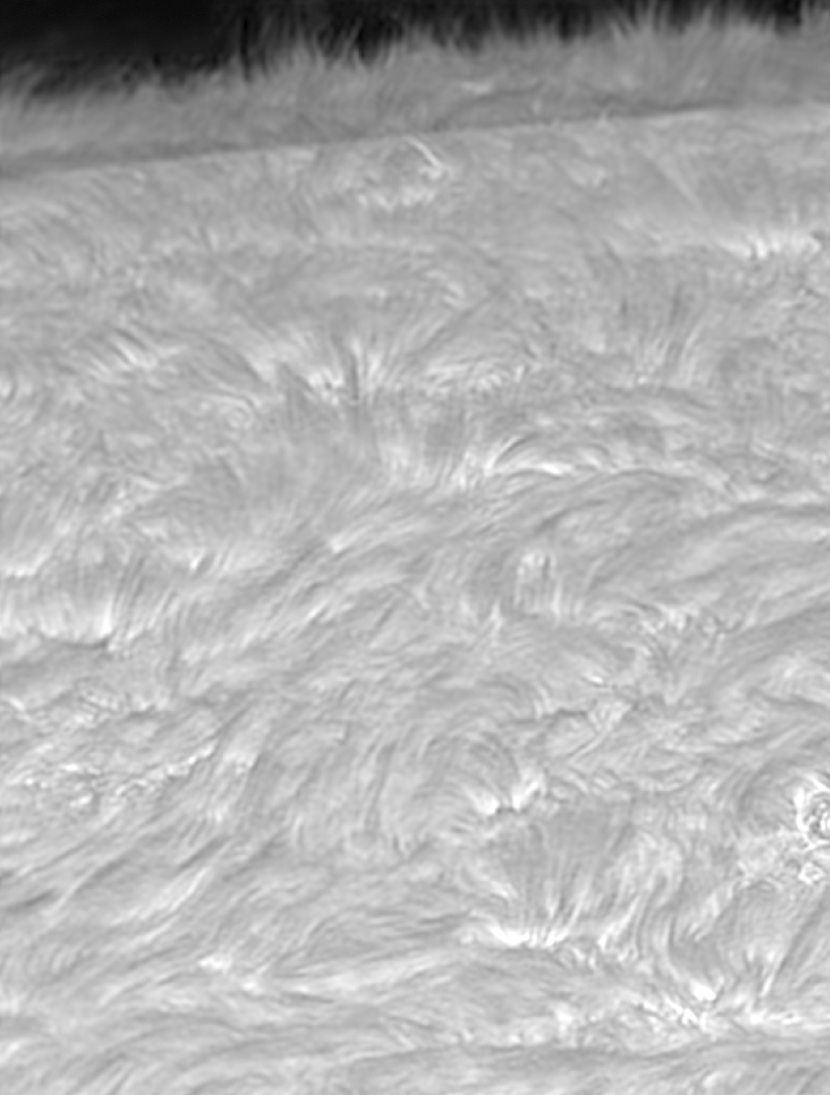
Figure 1: DOT limb image taken on 2005 October 4 at 09:38:40 UT in the H$\alpha$ line center. Field of view: $66\times 87$ arcsec².

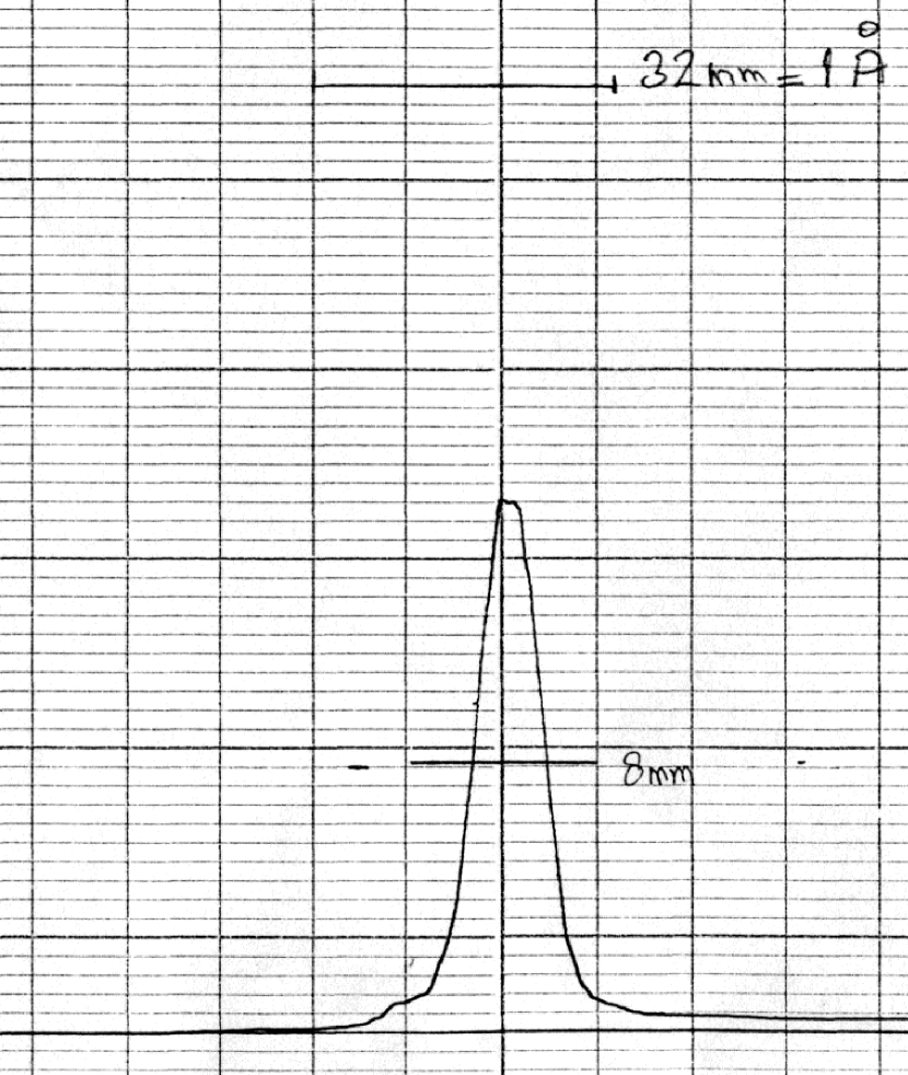
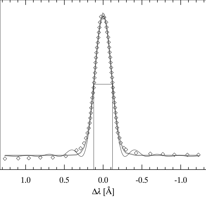
Figure 2: Top: scanned registration from ink recorder showing measured transmission profile of the DOT H$\alpha$ Lyot filter. Distance of vertical lines corresponds to 10 mm. The wavelength scale 32 mm $=1$ Å is handwritten in the upper right corner. Filter FWHM of 250 mÅ is marked by the horizontal line followed by the flank-to-flank distance of 8 mm. Bottom: digitized transmission profile of the DOT H$\alpha$ Lyot filter (diamonds), its Gaussian fit (thick gray line), and corresponding sinc² function (black line, Eq. (2)). Thin lines mark Gaussian FWHM of 243 mÅ.

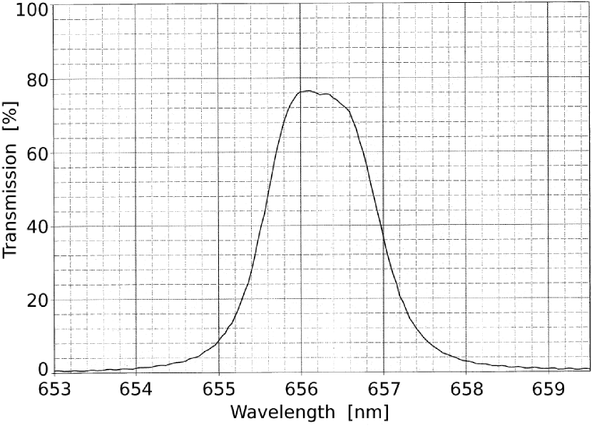
Figure 3: Transmission of prefilter of the DOT H$\alpha$ Lyot filter.

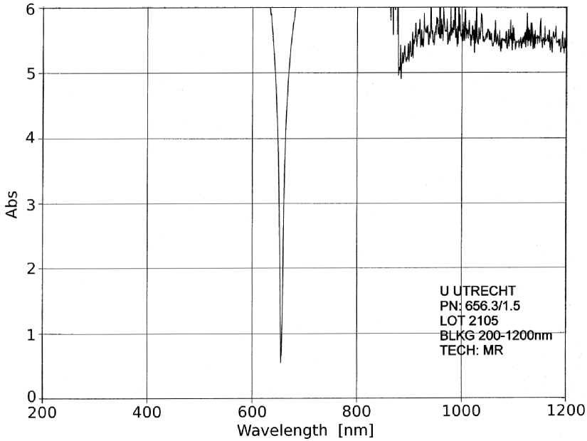
Figure 4: Absolute value of the logarithm to base 10 of the prefilter transmission in Fig. 3 over a broad spectral region. The transmission decreases upward.

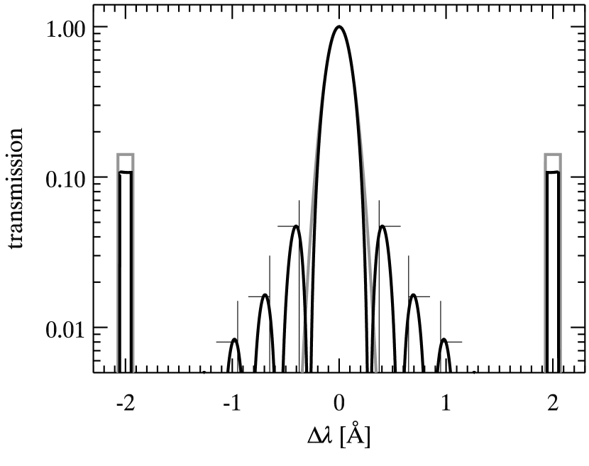
Figure 5: The theoretical transmission profiles of the DOT H$\alpha$ Lyot filter in the logarithmic scale: Gaussian $+\Lambda$ (gray) and sinc${}^{2}+\Pi$ (black), both with FWHM = 250 mÅ. The thin vertical lines with horizontal dashes approximately at $\pm 0.4,\pm 0.65$, and $\pm 0.95$ Å are the theoretical positions and the amplitudes of the subsidiary maxima according to Gaizauskas (1976, p. 8).

2 Spectroscopic investigation versus limb observation

The convolved intensity $E(\lambda)$ of incident light with a spectrum $I$ passing through a filter with a transmission profile $T$ centered at the wavelength $\lambda$ is the convolution

$$E(\lambda)=\int_{0}^{\infty}I(x)T(x-\lambda)dx\,.$$ (1)

For an application of a Lyot filter as a spectroscopic device and follow-up quantitative interpretation of observed $E(\lambda)$, e.g., through comparison with a synthetic spectrum $I$, one needs to assume or to know the transmission profile $T$ and its possible variations with tuning of the filter.

Table 1: Column 1: ratios of convolved intensities $E(\Delta\lambda)$. Parenthesis $\langle\,\rangle$ indicate an average of intensities at $\Delta\lambda$. Columns 2–4: observed ratios of spatio-temporal means of DOT H$\alpha$ datacubes obtained in the quiet Sun in the indicated days and average ratios of observations from 12 days. Columns 5–8: anticipated ratios computed by the atlas H$\alpha$ profile and the particular transmission profile with FWHM = 250 mÅ centered at $\Delta\lambda=0,\pm 0.35$, and $\pm 0.7$ Å from the center of the atlas profile. The symbols $\Lambda$ and $\Pi$ represent two rectangle add-ons of the Gaussian and sinc² function, respectively. See text and Fig. 5.

Ratio	DOT H$\alpha$ Observations			Atlas H$\alpha$ Profile + Transmission Profile:
	2005 Oct 19	2007 Sep 28	12-days average	Gauss	Gauss $+\,\Lambda$	sinc2	sinc${}^{2}+\Pi$
$\langle E(\pm 0.7)\rangle/E(0)$	2.32	2.34	2.34	3.28	2.35	2.78	2.35
$\langle E(\pm 0.7)\rangle/\langle E(\pm 0.35)\rangle$	1.75	1.75	1.75	2.10	1.77	1.94	1.76
$\langle E(\pm 0.35)\rangle/E(0)$	1.33	1.34	1.34	1.56	1.33	1.43	1.34

The DOT H$\alpha$ Lyot filter contains eight stages assembled from three groups of birefringent quartz crystals and five groups of calcite crystals (Bettonvil et al. 2006). Its transmission profile was measured photometrically in 1999 by the solar spectrograph in Sonnenborgh observatory in Utrecht (top panel of Fig. 2). The measurement confirmed almost symmetric and Gaussian-like transmission profile with the full width at half maximum FWHM = 250 mÅ without significant subsidiary maxima or far-center sidelobes ruling out a leakage of unwanted parasitic light. It also confirmed invariance of the profile in tuning. The bottom panel of Fig. 2 displays a digitized profile and its Gaussian fit (thick gray line) with FWHM = 243 mÅ. Note that the wavelength increases from the right to the left and there is no transmission scale since the measurement was not absolutely calibrated. In the service deployment at DOT, the filter is preceded by a prefilter with FWHM = 14.9 Å blocking out sidebands 128 Å apart from the central transmission peak (Bettonvil et al. 2006). The latter value is the free spectral range (FSR) of the filter. The transmission profile of the prefilter delivered by its manufacturer is shown in Figs. 3 and 4 for the narrow and broad spectral range. Note in the latter figure the broadband transmission of $10^{-5.5}$ in the IR spectral range spanning from 870 to 1200 nm.

On the contrary, Rutten (2007, 2012, 2013) admits presence of parasitic continuum light in DOT H$\alpha$ images pointing to the double limb (Rutten 2007) and the sharp limb (Rutten 2013) seen in the image taken in the H$\alpha$ line center (Fig. 1). In the figure the limb shines clearly through the mass of spicules. Visibility of the limb arc is highlighted by the dark band of variable width demarcating its outer limit. The dark band and the limb visibility in the H$\alpha$ line center images taken by a Lyot filter have already been described in Bray & Loughhead (1974) identifying the latter as a symptom of parasitic light. Suspicion of possible contamination of the DOT H$\alpha$ line center images by the parasitic continuum light may rise if comparing Fig. 1 with a limb image taken in the H$\alpha$ center by a Fabry-Pérot instrument. An example is the lower right panel of Fig. 6 in Puschmann et al. (2006) where the limb and the dark band are much less apparent. Nevertheless, more similar images taken with various Fabry-Pérot instruments at several position angles along the limb would be needed for comparison.

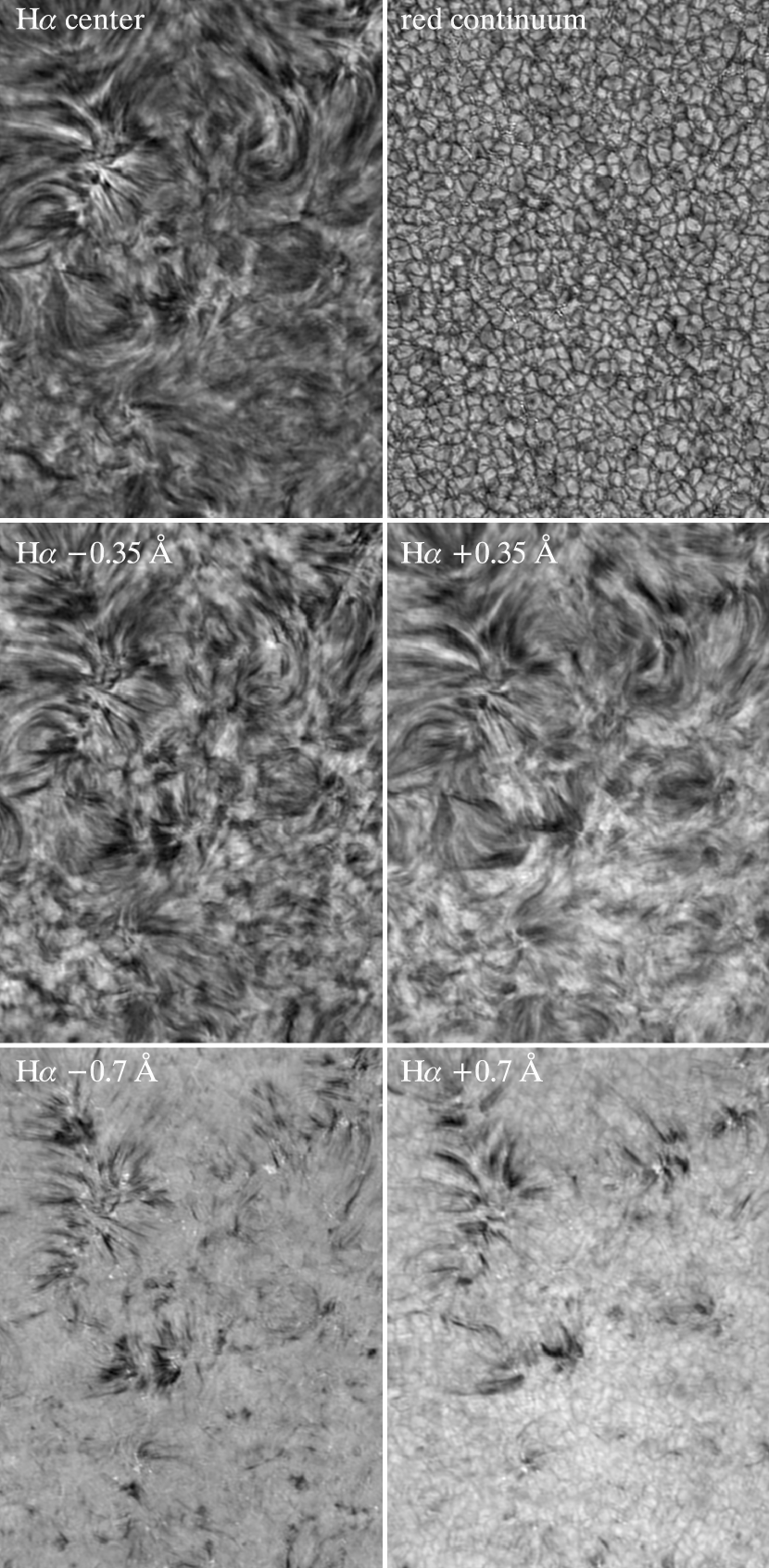
Figure 6: Sample H$\alpha$ images of the quiet Sun at the disk center recorded by DOT with the Hitachi KP-F100 camera with Sony ICX085 CCD sensor (Rutten et al. 2004) on 2005 October 19 at 10:36:21 UT at the moment of the best seeing occurred in the $41^{\rm st}$ minute after the beginning of the observation at 09:55:20 UT. Field of view: $58\times 79$ arcsec².

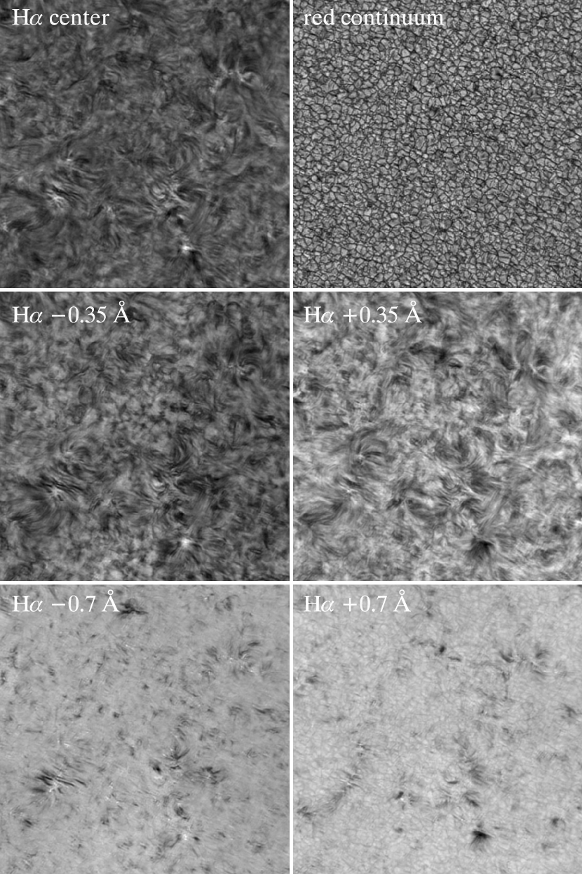
Figure 7: Sample H$\alpha$ images of the quiet Sun at the disk center recorded by DOT with the Redlake MegaPlus II ES4020 camera with Kodak KAI-4020 sensor on 2007 September 28 at 09:28:29 UT at the moment of the best seeing occurred in the $53^{\rm rd}$ minute after the beginning of the observation at 08:35 UT. Field of view: $93\times 93$ arcsec².

3 Towards new transmission profiles

In this section we perform a quantitative indirect testing of the transmission of the DOT H$\alpha$ filter represented by the Gaussian with FWHM = 250 mÅ (Fig. 2) and a square of normalized sinc function (from Latin sinus cardinalis, Fig. 5) as suggested in Gaizauskas (1976). The latter is an approximation for transmission of a single peak (see Appendix A) having the form

$${\rm sinc}^{2}(\Delta\lambda)=\left(\frac{\sin\pi x}{\pi x}\right)^{2},$$ (2)

where $x=2k\frac{\Delta\lambda}{\rm FWHM},\Delta\lambda$ is a distance from the center of the passband, and the transcendental equation $(\sin\pi k)^{2}/(\pi k)^{2}=0.5$ yields the conversion factor $k=0.442946$ between $x,\Delta\lambda$, and FWHM/2. Since the function has a singularity at $x=0$, its definition sets sinc${}^{2}(0)=1$ for $\Delta\lambda=0$.

First, we perform a simple check whether these theoretical transmission profiles are compatible with observations. To this purpose, we have chosen the H$\alpha$ observations of very quiet areas at the disk center available in the DOT database taken on 2005 October 19 and 2007 September 28 at the H$\alpha$ line center and at $\pm 0.35$ and $\pm 0.7$ Å off the center (Figs. 6 and 7). Quietness of the target areas is documented by the continuum images taken simultaneously by a broadband interference filter with FWHM = 2.4 Å centered at 6550.5 Å. The datasets differ mainly in type of cameras used. We computed the spatio-temporal mean of each datacube at the employed wavelength positions of the filter and the ratios as defined in Col. 1 of Table 1. Columns 2 and 3 show that these ratios are independent of type of camera. They are also insensitive to the area averaged since they do not change much if only large internetwork areas are adopted for averaging. We checked also invariability of the ratios with time taking single quiet-Sun H$\alpha$ scans at the disk center from twelve days mostly in 2007. Spans of the ratios are 2.25–2.44, 1.70–1.79, and 1.32–1.37 with averages given in Col. 4.

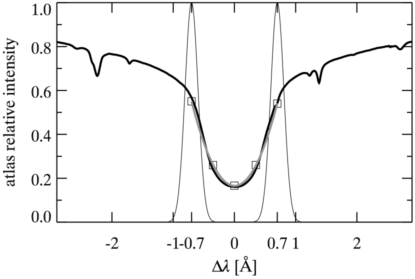
Figure 8: Intensities (squares) obtained by convolution of the atlas H$\alpha$ profile (thick black) and the Gaussian transmission profile with FWHM = 250 mÅ centered at $0,\pm 0.35$, and $\pm 0.7$ Å (the last two shown as thin solid) together with a parabolic fit (gray) of the intensities.

Columns 5 and 7 of Table 1 show anticipated ratios for the H$\alpha$ profile extracted from the spectral atlas (Neckel 1999) and convolved with the Gaussian and sinc² function. Apparently, these models of the transmission profile yield ratios significantly exceeding the observed ones. It suggests in sharp contradiction with the result of measurement in 1999 that the real transmission profile of the DOT H$\alpha$ filter might have larger throughput than these models and lets in some parasitic continuum light contaminating mainly the core and thus decreasing the observed ratios compared to the anticipated ones. This is illustrated plainly in Figs. 8 and 9 as the shallowing of the observed H$\alpha$ core. Then the additional continuum light in limb images taken in the H$\alpha$ center increases significantly the limb contrast with respect to off-limb emission structures (Fig. 1) shining on the background of scattered continuum light.

Table 2: Rectangle parameters.

Rectangle	Area	Width	Height
	(mÅ)	(mÅ)
$\Lambda$	20.0	141	0.141
$\Pi$	11.5	107	0.107

To account for the missing parasitic light, we constructed two models combining the Gaussian and sinc² function (Eq. 2) with two ad hoc rectangle functions $\Lambda$ and $\Pi$ (Fig. 5) centered at $\Delta\lambda=\pm 2$ Å around the H$\alpha$ line center. The symbols $\Lambda$ and $\Pi$ indicate the light leak and the shape of the functions. The areas of rectangles were found by a trial and error (Cols. 6 and 8 of Table 1) to match the observed ratios. Parameters of a single rectangle are summarized in Table 2. These extensions of Gaussian and Eq. (2), referred as Gauss $+\,\Lambda$ and sinc${}^{2}+\Pi$, represent new theoretical transmission profiles of the DOT H$\alpha$ Lyot filter accounting for the sharp limb in Fig. 1 and reconciling discrepancies between anticipated and observed intensity ratios in Table 1. The integrals of the Gaussian and sinc² function, both with FWHM = 250 mÅ, are 266 and 282 mÅ (Appendix B). For comparison, the rectangle add-ons increase their areas about $40\times 100/266=15\%$ and $23\times 100/282=8\%$.

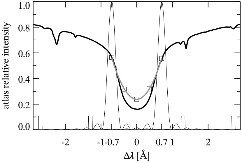
Figure 9: The same as in Fig. 8 but for the theoretical transmission profile sinc${}^{2}+\Pi$.

4 Discussion

Our study points out the striking discrepancy between the observed and anticipated intensity ratios shown in Cols. 2–4 and Col. 5 of Table 1 assuming the Gaussian transmission profile in concert with the measured Gaussian-like sidelobe-free transmission of the DOT H$\alpha$ Lyot filter (Fig. 2). Column 7 of Table 1 indicates some alleviation of the discrepancy for the sinc² function (Fig. 5) suggested in Gaizauskas (1976). Is it all truly an another manifestation of parasitic continuum light visible in Fig. 1 as the sharp limb as suggested in Rutten (2007, 2012, 2013)?

On the suggestion of a referee, we discuss separately two likely leaks of the parasitic light. These are the broadband transmission of $10^{-5.5}$ of the prefilter in IR spanning from 870 to 1200 nm (Fig. 4) and/or the main passband of the Lyot filter itself. Since original IR cut filters were dismantled from DOT cameras prior their deployment and assuming that the DOT optics is fully transparent in IR, the leak can be represented as an extension of the right side of Eq. (1) by $\varepsilon=\varepsilon_{\rm VIS}+\varepsilon_{\rm IR}$, where $\varepsilon$ is the total area of rectangles in Table 2. Then $\varepsilon_{\rm VIS}$ and $\varepsilon_{\rm IR}$ are the light leak through the main passband of the filter and the IR leak of the prefilter. The latter can be estimated by the formula

$$\varepsilon_{\rm IR}=\frac{F_{\rm IR}}{F_{\rm H\alpha}}\frac{P_{\rm IR}}{P_{\rm H\alpha}}\frac{S_{\rm IR}}{S_{\rm H\alpha}}\frac{\Delta\lambda_{\rm IR}}{FSR}\int_{0}^{\infty}T(\lambda)d\lambda\,,$$ (3)

where $F_{\rm IR}$ and $F_{\rm H\alpha}$ are the average solar fluxes in IR and the H$\alpha$ continuum in the DOT altitude of 2350 m for the specific solar zenith angle. We computed their ratio of 0.45 by the radiative transfer library libRadtran (Mayer & Kylling 2005). The factor $P_{\rm IR}/P_{\rm H\alpha}$ is the ratio of the average transmissions of the prefilter in IR and H$\alpha$ estimated from Figs. 3 and 4 as $10^{-5.5}/0.76\approx 4\times 10^{-6}$. The next factor $S_{\rm IR}/S_{\rm H\alpha}$ accounts for different sensitivity of DOT cameras in IR and H$\alpha$. We estimated its value of 0.12 from curves of spectral sensitivity of their sensors showing that their efficiency has a cut off at 1000 nm. The last but one factor $\Delta\lambda_{\rm IR}/FSR\approx 10$ is the number of sidebands of the Lyot filter with $FSR=12.8$ nm and the integrated transmission of $\int_{0}^{\infty}T(\lambda)d\lambda=282$ mÅ within the considered spectral range of $\Delta\lambda_{\rm IR}=1000-870=130$ nm. The product of these factors is $\varepsilon_{\rm IR}\approx 6.5\times 10^{-4}$ mÅ.

Consider now the extreme but unlikely situation that the polarizers in the Lyot filter are completely ineffective in infrared wavelengths, i.e., transmit all polarization directions equally, rendering the Lyot filter ineffective. Then Eq. (3) simplifies to the form

$$\varepsilon_{\rm IR}=\frac{F_{\rm IR}}{F_{\rm H\alpha}}\frac{P_{\rm IR}}{P_{\rm H\alpha}}\frac{S_{\rm IR}}{S_{\rm H\alpha}}\Delta\lambda_{\rm IR}\,,$$ (4)

where the last factor $\Delta\lambda_{\rm IR}=130$ nm accounts for complete ineffectiveness of the Lyot filter in the wavelength range from 870 to 1000 nm. For this extreme situation, we find that $\varepsilon_{\rm IR}=0.3$ mÅ which is only 1.3% of the total area of 23 mÅ of two correcting $\Pi$ rectangles (Table 2) proving that

• the IR leak of the prefilter is negligible compared to $\varepsilon$ listed in Table 2 in the Area column,

• virtually all parasitic light leaks through the main passbands of the prefilter and the Lyot filter.

For the latter, we can imagine the following possible source and cause of the parasitic light

• the central peak of the transmission profile is superimposed on the background of very low transmission spanning over the whole spectrum,

• the transmission profile has changed since its measurement in 1999 and a new measurement would be needed.

The two rectangle add-ons of the Gaussian and sinc² functions (Fig. 5) thus compensate for these effects or their combination. A possible non-linearity of the cameras as a cause is excluded since almost the same ratios are obtained for datasets taken by different cameras (Figs. 6 and 7, Cols. 2 and 3 in Table 1). Since the transmission measurement was not absolutely calibrated (Fig. 2), the level of background transmission is unknown. Nevertheless, a closer inspection of the top panel of Fig. 2 suggests an increased background transmission extending blueward from the peak. This may contribute significantly to the total amount of parasitic light.

Deviations in the relative rotational orientation of the eight successive stages (Bettonvil et al. 2006) of the Lyot filter can be the source of the blue-ward background. It did not change in value and shape when the filter was tuned from $-1.5$ to $+1.5$ Å. This means that these deviations occur in the initial rotational orientation of the stages and do not change with the rotations for tuning, each next stage with double speed of the preceding stage performed by traditional toothed gear-wheels assuring no change in their relative positions by tuning many times forward and backward.

The transmission curves of the 1999 measurements were scanned in the spectrum using a moving slit with photomultiplier, which was sending its signal to a recorder. The scanned curves were about 4 Å broad with the transmission peak near the center. Consequently, the indication of the blue-ward background is only visible till 2 Å from the transmission peak. The transmission region of the prefilter is much broader, see Fig. 3. It is possible that there is a red-side background further away from the transmission peak of the Lyot filter. It can be caused by combinations of orientation deviations of stages of higher and lower path differences between the polarization directions. Consequently, the chosen correction with two ad hoc rectangular functions at 2-Å distance from the transmission peak, well within the transmission range of the prefilter, is rational.

Limb H$\alpha$ images taken by a Fabry-Pérot instrument (FPI) offer a possibility to simulate an influence of the parasitic light on appearance of limb in DOT H$\alpha$ line center images like Fig. 1. The contamination can be simulated by summing of FPI H$\alpha$ line center image with an FPI continuum image but weighted appropriately. After some trial and errors one should arrive to a small factor producing a sharp limb in the FPI H$\alpha$ line center image. We plan to perform this test in the future with images obtained by some of high-performance Fabry-Pérot instruments. The most-probable source is the Interferometric Bidimensional Spectrometer (Cavallini 2006) installed at the Dunn Solar Telescope. Its open database already offers potentially usable datasets taken in the service mode in the first months of 2013.

5 Conclusions

In this paper we summarize available facts about the transmission profile of the DOT H$\alpha$ Lyot filter. Its accurate knowledge is important, in particular in comparing observations with simulated data as was carried out in Leenaarts et al. (2006). While the spectroscopic measurement in 1999 showed almost symmetric and Gaussian-like transmission profile without significant subsidiary maxima or far-center sidelobes, two indirect and entirely different approaches indicate possible leakage of parasitic continuum light into DOT H$\alpha$ images. To reconcile the discrepancy, we suggest two theoretical transmission profiles of the DOT H$\alpha$ Lyot filter combining the Gaussian and sinc² functions (Eq. 2) with two ad hoc rectangle functions. The extended Gauss$\,+\,\Lambda$ and sinc${}^{2}+\Pi$ functions are equivalent. The former is simpler in use while the latter conforms the theory (see Appendix A) but has a singularity at $x=0$. These functions should be considered only as the best available approximations usable in relevant applications. Decisive answer can give only spectroscopic re-measurement of the transmission profile of the DOT H$\alpha$ Lyot filter yielding calibrated transmission.

Appendix A Mathematical background

Lyot (1944, p. 7) and Stix (2004, p. 107) show that an incident wave with the amplitude $A$ and the wavelength $\lambda$ exits from an $N$-stage Lyot filter with the amplitude $A^{\prime}$

$$A^{\prime} = A\cos\frac{\pi eJ}{\lambda}\cos\frac{2\pi eJ}{\lambda}\cos\frac{4\pi eJ}{\lambda}~{}\cdots~{}\cos\frac{2^{N-1}\pi eJ}{\lambda}$$ (5)

$$= A\prod_{k=1}^{N}\cos\frac{2^{k-1}\pi eJ}{\lambda}\,,$$

where $e$ is the thickness of the first crystal plate with the birefringence $J$. Lyot (1944, p. 7), van Griethuysen & Houtgast (1959, p. 279), Title & Rosenberg (1981, p. 816), and Bland-Hawthorn et al. (2001, p. 615) express the exit amplitude $A^{\prime}$ in the form

$$A^{\prime}=A\;\frac{\sin 2^{N}\frac{\pi eJ}{\lambda}}{2^{N}\sin\frac{\pi eJ}{\lambda}}\,.$$ (6)

We adopt in Eqs. (5) and (6) the same notation as Stix (2004). Finally, Gaizauskas (1976, p. 8) approximates the exit amplitude $A^{\prime}$ for a single peak with the formula

$$A^{\prime}=A\;\frac{\sin\pi x}{\pi x}\,.$$ (7)

Since we did not find in available literature a derivation of Eqs. (6) and (7), we show it here. Repeated use of the double angle formula for the sine shows that

$$\sin 2^{1}x = 2^{1}\sin x\cos x\,,$$

$$\sin 2^{2}x = 2^{2}\sin x\cos x\cos 2x\,,$$

$$\sin 2^{3}x = 2^{3}\sin x\cos x\cos 2x\cos 2^{2}x\,,$$

$$\sin 2^{4}x = 2^{4}\sin x\cos x\cos 2x\cos 2^{2}x\cos 2^{3}x\,,$$

$$\vdots$$

$$\sin 2^{N}x = 2^{N}\sin x\prod_{k=1}^{N}\cos 2^{k-1}x\,.$$ (8)

Then the product of the cosines is

$$\prod_{k=1}^{N}\cos 2^{k-1}x=\frac{\sin 2^{N}x}{2^{N}\sin x}\,,$$ (9)

proving Eq. (6) for $x=\pi eJ/\lambda$ .

Let $E=2^{N}e=2\times 2^{N-1}e$ is a doubled thickness of the $N$th crystal plate of a Lyot filter (Stix 2004). Exchanging $e$ for $E$ in Eq. (6) one can obtain

$$A^{\prime}=A\;\frac{\sin\frac{\pi EJ}{\lambda}}{2^{N}\sin\frac{\pi EJ}{2^{N}\lambda}}\,.$$ (10)

The limit of the right side of Eq. (10) for $N\to\infty$ is

$$\lim_{N\to\infty}\frac{\sin\frac{\pi EJ}{\lambda}}{2^{N}\sin\frac{\pi EJ}{2^{N}\lambda}}=\frac{\sin\frac{\pi EJ}{\lambda}}{\lim\limits_{N\to\infty}2^{N}\sin\frac{\pi EJ}{2^{N}\lambda}}=\frac{\sin\frac{\pi EJ}{\lambda}}{\frac{\pi EJ}{\lambda}}\,,$$ (11)

proving Eq. (7) for $x=\frac{EJ}{\lambda}$, because $\lim\limits_{N\to\infty}2^{N}\sin\frac{X}{2^{N}}=X$ (see, e.g., Morrison 1995).

Thus the single-peak approximation introduced in Gaizauskas (1976) represents a hypothetical Lyot filter with infinite number of stages with the full width at half maximum

$${\rm FWHM}=0.88\frac{\lambda^{2}}{EJ}$$ (12)

(see, e.g., Title & Rosenberg 1981) but with the thickness of the thinnest plate $e$ approaching to zero resulting in an infinitely-large free spectral range defined in Title & Rosenberg (1981) as

$${\rm FSR}=\frac{\lambda^{2}}{eJ}\,.$$ (13)

Appendix B Useful integrals

$$\int_{0}^{\infty}e^{-(ax)^{2}}dx=\frac{\sqrt{\pi}}{2a}$$ (14)

$$\int_{0}^{\infty}\frac{\sin^{2}(ax)}{x^{2}}dx=\frac{\pi}{2}|a|$$ (15)