On the power divergence in quasi gluon distribution function

Abstract

Recent perturbative calculation of quasi gluon distribution function at one-loop level shows the existence of extra linear ultraviolet divergences in the cut-off scheme. We employ the auxiliary field approach, and study the renormalization of gluon operators. The non-local gluon operator can mix with new operators under renormalization, and the linear divergences in quasi distribution function can be into the newly introduced operators. After including the mixing, we find the improved quasi gluon distribution functions contain only logarithmic divergences, and thus can be used to extract the gluon distribution in large momentum effective theory.

I Introduction

The high energy behaviour of a hadron is encoded into parton distribution functions (PDFs). Because of the non-perturbative nature, the PDFs can not be calculated in QCD perturbation theory. Traditionally, PDFs are extracted using the experimental data for the processes in which the factorization theorem is established Butterworth:2015oua ; Hou:2016nqm ; Hou:2017khm ; Gao:2017yyd . Another popular non-perturbative method is to use lattice QCD (LQCD). However, since PDFs are defined as light-cone correlation matrix elements Collins:2011zzd , it is a formidable task to calculate the PDFs on the lattice. Instead only the lowest few moments are explored due to the technical difficulties.

A novel approach, named as large momentum effective theory (LaMET), has been proposed to extract light-cone observables from lattice calculation Ji:2013dva ; Ji:2014gla . In this approach, one can calculate the corresponding quasi observables on the lattice, defined by equal-time correlation matrix elements. The quasi and light-cone observables share the same infrared (IR) structures. The difference between them is IR independent, and can be calculated perturbatively. Factorization of the quasi quark distribution has been examined at one-loop level and proved to hold to all orders Xiong:2013bka ; Ma:2014jla . Therefore, if the matching coefficient is calculated in perturbation theory, and the quasi distribution function is evaluated on the lattice, one can extract light-cone distribution functions. This approach has been studied extensively Gamberg:2014zwa ; Ji:2014hxa ; Jia:2015pxx ; Ji:2015qla ; Ji:2015jwa ; Monahan:2015lha ; Xiong:2015nua ; Gamberg:2015opc ; Ishikawa:2016znu ; Monahan:2016bvm ; Bacchetta:2016zjm ; Ji:2017rah ; Nam:2017gzm ; Rossi:2017muf ; Stewart:2017tvs ; Xiong:2017jtn ; Hobbs:2017xtq ; Broniowski:2017wbr ; Carlson:2017gpk ; Chen:2017mie ; Monahan:2017hpu , and some encouraging progresses on LQCD calculation are reported Lin:2014zya ; Alexandrou:2015rja ; Chen:2016utp ; Alexandrou:2017huk ; Lin:2017ani ; Briceno:2017cpo ; Chen:2017mzz ; Constantinou:2017sej ; Zhang:2017bzy . Some other frameworks, e.g., the pseudo-PDFs Radyushkin:2016hsy ; Radyushkin:2017cyf ; Radyushkin:2017ffo ; Radyushkin:2017gjd ; Orginos:2017kos ; Karpie:2017bzm ; Radyushkin:2017lvu and the “lattice cross section” approach Ma:2014jla ; Ma:2014jga ; Ma:2017pxb are also developed.

The one-loop calculations of matching coefficient in the cutoff scheme show that, the quasi quark PDF contains linear power ultraviolet (UV) divergences Xiong:2013bka . These divergences arise from Wilson-line’s self-energy. Some suggestions have been made to solve the problem, e.g., the non-dipolar Wilson line Li:2016amo ; Li:2017udt , a mass counter term of Wilson line Chen:2016fxx , as well as the auxiliary field formalism Green:2017xeu . All these methods are based on the fact that the linear power divergences arise from Wilson lines’ self-energy diagram. The renormalizability of quasi quark distribution has also been proved to all orders recently Ji:2017oey ; Ishikawa:2017faj . Based on the multiplicative renormalizability of quasi-PDF, one can perform nonperturbative renormalization of quasi-PDF in the regularization-invariant momentum-subtraction (RI/MOM) scheme Martinelli:1994ty , in which the UV divergence can be removed to all orders by a renormalization factor determined on the lattice Chen:2017mzz ; Green:2017xeu ; Lin:2017ani ; Stewart:2017tvs .

Among various PDFs, the gluon distribution function is a key quantity especially for the processes like the production of Higgs particles. It is also crucial for understanding the spin structure of hadron. However, compared to the quasi quark distribution, the quasi gluon distribution is less explored. A first calculation of perturbative coefficient for quasi gluon distribution is presented in Ref. Wang:2017qyg , in which the results are presented in both the cut-off and dimensional regularization (DR) schemes. It is shown that linear divergences exist even in the diagrams without any Wilson line, and thus these linear divergences can not be absorbed into the renormalization of Wilson line. Hence the gluon quasi PDF is much more involved. In this work we focus on power divergences in quasi gluon distribution. We will show that, in the formalism of auxiliary field, the linear divergences can be renormalized by considering the contribution from possible operator mixing, as well as the mass counter term of Wilson line.

The rest of this paper is organized as follows. In Sec. II, we introduce a slightly modified definition of quasi gluon distribution. In Sec. III, we present the perturbative calculation of quasi gluon distribution at one-loop level. In Sec. IV, the renormalization of linear divergence will be analyzed with auxiliary field method. Then we propose an improved quasi gluon distribution and calculate the matching coefficient in Sec. V. Sec. VI is the summary and outlook of this work. In the appendix, we give some detailed calculations of the real diagrams with no Wilson lines involved.

II Definition of quasi gluon distribution

The light-cone (or conventional) gluon distribution function is defined by a non-local matrix element of two light-cone separated gluon strength tensor

$$f_{g/H}(x,\mu)=\int\frac{d\xi^{-}}{2\pi xP^{+}}e^{-i\xi^{-}xP^{+}}\langle P|G^{+}_{~{}i}(\xi^{-}n_{+})W(\xi^{-}n_{+},0;L_{n_{+}})G^{i+}(0)|P\rangle.$$ (1)

In the light-cone coordinate, a four-vector $a$ is expressed as $a=(a^{+},a^{-},\vec{a}_{\perp})$, with $a^{+}=(a^{0}+a^{z})/\sqrt{2}$ and $a^{-}=(a^{0}-a^{z})/\sqrt{2}$. $n_{+}=(0,1,0,0)$ is a light-cone vector. Similarly, the quasi gluon distribution can be defined by non-local matrix element which is equal-time separated Ji:2013dva ; Ma:2017pxb ; Wang:2017qyg

$$\tilde{f}_{g/H}(x,P^{z})=\int\frac{dz}{2\pi xP^{z}}e^{izxP^{z}}\langle P|G^{z}_{~{}i}(zn_{z})W(zn_{z},0;L_{n_{z}})G^{iz}(0)|P\rangle.$$ (2)

In quasi PDF we still adopt the Cartesian coordinates, where $n^{\mu}_{z}=(0,0,0,1)$ is an unite vector along $z$ direction. In the above definitions, $W(x,y;C)$ denotes a Wilson line along contour $C$ with two endpoints $x$ and $y$, the gluon field is in adjoint representation and $L_{n}$ is a straight line with direction vector $n$. The Wilson line can be parametrized as

$$W(z_{1},z_{2},L_{n})=P\exp\left[-ig\int^{1}_{0}d\lambda~{}\dot{x}(\lambda)\cdot A(x(\lambda))\right],$$ (3)

where $P$ denotes that the operator exponential is path ordered. Any point on $L_{n}$ can be expressed as $x(\lambda)=\bar{\lambda}z_{2}n+\lambda z_{1}n$, where $\bar{\lambda}\equiv 1-\lambda$, $x(0)=z_{2}n$ and $x(1)=z_{1}n$. $\dot{x}^{\mu}(\lambda)\equiv dx^{\mu}(\lambda)/d\lambda$ is the velocity vector of the contour.

According to Refs. Ji:2013dva ; Ma:2017pxb ; Wang:2017qyg , $i$ sums over the transverse directions. In this paper, we adopt a modified definition, where the Lorentz index of gluon field strength tensor is summed over all the directions except “3”, i.e.,

$$\tilde{f}_{g/H}(x,\mu)=\int\frac{dz}{2\pi xP^{z}}e^{izxP^{z}}\langle P|G^{z}_{~{}{\mu}}(zn_{z})W(zn_{z},0;L_{n_{z}})G^{\mu z}(0)|P\rangle\ ,$$ (4)

for $\mu=0,1,2$.

To see that Eq. (4) is a proper definition of quasi gluon distribution, we begin with the energy-momentum tensor of gluon field

$$T^{\mu\nu}=G^{\mu\lambda}G_{\lambda}^{~{}\nu}-\frac{1}{4}g^{\mu\nu}G^{\alpha\beta}G_{\beta\alpha}.$$ (5)

The averaged value of $T^{\mu\nu}$ between a hadron state $|P\rangle$ can be expressed as

$$\langle P|T^{\mu\nu}|P\rangle=a(\mu)\left(P^{\mu}P^{\nu}-\frac{1}{4}M^{2}g^{\mu\nu}\right),$$ (6)

in which $M$ is the hadron mass. This tensor is symmetric and traceless with a scalar function $a(\mu)$ characterizing the magnitude. If we pick up the “$++$” component, i.e. $\mu=\nu=+$, we have

$$\langle P|T^{++}|P\rangle=a(\mu)(P^{+})^{2}.$$ (7)

The term proportional to $M^{2}$ disappears because $g^{++}=0$. On the other hand, if we take $\mu=\nu=z$, then

$$\langle P|T^{zz}|P\rangle=a(\mu)\left[(P^{z})^{2}-\frac{1}{4}g^{zz}M^{2}\right]=a(\mu)\left[(P^{z})^{2}+\frac{1}{4}M^{2}\right]=a(\mu)(P^{z})^{2}\left(1+O(M^{2}/(P^{z})^{2})\right).$$ (8)

Eqs. (7) and (8) are related to the first moment of light-cone and quasi gluon distribution respectively,

$$\int dx~{}xf_{g/H}(x,\mu) =\frac{1}{(P^{+})^{2}}\langle P|T^{++}|P\rangle=a(\mu),$$ (9)

$$\int dx~{}x\tilde{f}_{g/H}(x,P^{z},\mu) =\frac{1}{(P^{z})^{2}}\langle P|T^{zz}+\frac{1}{4}g^{zz}G^{\alpha\beta}G_{\alpha\beta}|P\rangle+{O}\left(\frac{M^{2}}{(P^{z})^{2}}\right)=a(\mu)+{O}\left(\frac{\Lambda^{2}_{\mathrm{QCD}}}{(P^{z})^{2}},\frac{M^{2}}{(P^{z})^{2}}\right).$$ (10)

Under the $P^{z}\to\infty$ limit, one can obtain $\int dx~{}xf_{g/H}(x,\mu)=\int dx~{}x\tilde{f}_{g/H}(x,P^{z},\mu)$. This relation can be generalized to high order moments, and consequently, to the distribution functions $f$ and $\tilde{f}$ themselves. It indicates that Eq. (4) is a reasonable definition of quasi gluon distribution. As a comparison, if $\lambda$ is only summed over transverse directions in Eq. (5), the tensor will not be Lorentz covariant, and then the above arguments will no longer hold.

Actually, one can easily validate that both definitions in Eqs. (2) and (4) will give the same results for the matching at tree-level. In addition, the non-local operator $G^{z}_{~{}{\mu}}(zn_{z})W(zn_{z},0;L_{n_{z}})G^{\mu z}(0)$ can be decomposed into the $\pm$ components:

$$G^{z}_{~{}{\mu}}(zn_{z})W(zn_{z},0;L_{n_{z}})G^{\mu z}(0)=\frac{1}{2}[G^{+}_{~{}{\mu}}(zn_{z})-G^{-}_{~{}{\mu}}(zn_{z})]W(zn_{z},0;L_{n_{z}})[G^{\mu+}(0)-G^{\mu-}(0)].$$ (11)

In the large $P^{z}$ limit, the $-$ component is suppressed and thus the operator for quasi-PDF recovers the same Lorentz structure with the light-cone PDF. The factor $1/2$ arises from the conversion of Euclidean and light-cone coordinates.

III One-loop corrections to quasi gluon distribution

Based on the definition in Eq. (4), we will re-calculate the one-loop correction to quasi gluon distribution. To perform the matching, one can replace the hadron state with a single parton state. In this paper we are interested in the gluon-in-gluon case. The hadron state $|P\rangle$ can be replaced by an on-shell gluon state $|g(P)\rangle$, where $P$ is the gluon momentum. To regulate the UV divergence, we introduce an UV cut-off $\Lambda$ on the transverse momentum. This cut-off corresponds to $1/a$ in LQCD, with $a$ being the lattice spacing. The collinear divergence is regulated by a small gluon mass $m_{g}$. We will perform the perturbative calculation in Feynman gauge.

The Feynman rules are listed in Fig. 1. The left two sub-diagrams are from the Abelian part of the gluon field strength tensor, while the right two are from the non-Abelian part. In these Feynman rules, we have explicitly separated the non-Abelian terms.

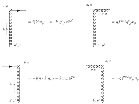
Figure 1: The Feynman rules for non-local vertex from gluonium operator. The left two sub-diagrams are from the Abelian part of the gluon field strength tensor, while the right two are from the non-Abelian part.

We firstly make some remarks on the self-energy corrections of the external gluon. It is known for a long time that the UV cut-off scheme (on all the components of internal momentum) leads to a quadratic divergence in QCD vacuum polarization diagram, which breaks the Ward identity and the gauge invariance. An exception is the lattice perturbation theory that provides an UV cut-off scheme which preserve the gauge invariance. For a detailed review on lattice perturbation theory, one can refer to Ref. Capitani:2002mp . The quadratic divergence in lattice perturbation theory will be canceled by additional tadpole-like diagrams, as well as the counter term which originates from the measure of the path integral. These diagrams are shown in Fig. 2, (a) has the continuum analog and diverge like $1/a^{2}$. This $1/a^{2}$ divergence corresponds to the quadratic divergence in continuum theory with a naive UV cut-off. The (b), (c) and (d) only exist in lattice theory but are essential to restore the gauge symmetry. One can set the same renormalization scales (or the UV cut-offs) for quasi and light-cone gluon distributions, then the gluon self energy diagram contributes a same factor to light-cone and quasi distributions, and will not contribute to the matching coefficient. Based on the above discussions, it is not necessary to include the gluon’s self energy at present.

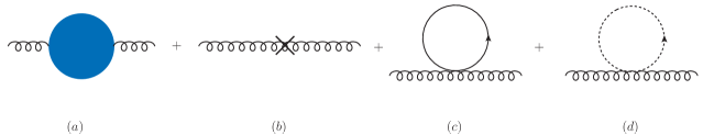
Figure 2: One-loop self energy diagrams of gluon in lattice perturbation theory. (a) denote the diagrams which have corresponding diagrams in the continuous limit. (b) is a counter-term which arises from the measure of path integral. (c) and (d) are tadpole diagrams involving a quark or ghost loop, which only exist in lattice perturbation theory.

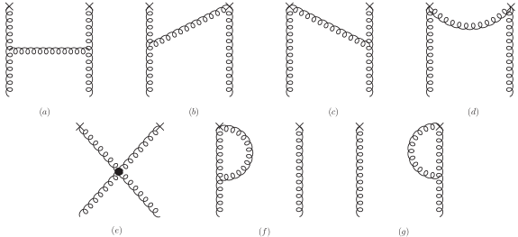
Figure 3: One-loop corrections to quasi gluon distribution without any Wilson line. The cross “$\times$” denotes the non-local vertex from the operator structure of definition.

We start with the calculation of one-loop diagrams with no Wilson line. The Feynman diagrams are shown in Fig. 3. In Fig. 3(a), the non-local vertex is from the Abelian term of field strength tensor. A direct calculation gives

$$x\tilde{f}_{g/g}^{(1)}(x,P^{z},\Lambda)\bigg{|}_{\mathrm{Fig}.\ref{fig:nowl}(a)} =\frac{\alpha_{s}C_{A}}{2\pi}\left\{\begin{aligned} &\left(2x^{3}-3x^{2}+2x-2\right)\ln\frac{x-1}{x}+2x^{2}-\frac{5x}{2}+3+\frac{\Lambda}{P^{z}}\ ,&x>1\\ &\left(2x^{3}-3x^{2}+2x-2\right)\ln\frac{(1-x+x^{2})m_{g}^{2}}{4x(1-x)(P^{z})^{2}}\\ &~{}~{}+\frac{(2x-1)(4x^{4}-6x^{3}+10x^{2}-5x+2)}{2(1-x+x^{2})}+\frac{\Lambda}{P^{z}},&0<x<1\\ &-\left(2x^{3}-3x^{2}+2x-2\right)\ln\frac{x-1}{x}-2x^{2}+\frac{5x}{2}-3+\frac{\Lambda}{P^{z}}\ .&x<0\end{aligned}\right.$$ (12)

Fig. 3(b, c) and (d) correspond to the contributions from the non-Abelian term in the field strength tensor. Note that in Ref. Wang:2017qyg , the non-Abelian term is combined with the Wilson line. In the present work, the contributions from these two parts are separated. This is more convenient to find the source of linear divergence. These diagrams give

$$x\tilde{f}_{g/g}^{(1)}(x,P^{z},\Lambda)\bigg{|}_{\mathrm{Fig}.\ref{fig:nowl}(b)}=\frac{\alpha_{s}C_{A}}{4\pi}\left\{\begin{aligned} &x(x+1)\ln\frac{x-1}{x}+2x-1-\frac{\Lambda}{P^{z}},~{}~{}~{}~{}&x>1\\ &x(x+1)\ln\frac{(1-x+x^{2})m^{2}_{g}}{4x(1-x)(P^{z})^{2}}+2x(x-1)+1-\frac{\Lambda}{P^{z}},~{}~{}~{}~{}&0<x<1\\ &-x(x+1)\ln\frac{x-1}{x}-2x+1-\frac{\Lambda}{P^{z}},~{}~{}~{}~{}&x<0\end{aligned}\right.$$ (13)

$$x\tilde{f}_{g/g}^{(1)}(x,P^{z},\Lambda)\bigg{|}_{\mathrm{Fig}.\ref{fig:nowl}(c)}=x\tilde{f}_{g/g}^{(1)}(x,P^{z},\Lambda)\bigg{|}_{\mathrm{Fig}.\ref{fig:nowl}(b)},$$ (14)

and

$$x\tilde{f}_{g/g}^{(1)}(x,P^{z},\Lambda)\bigg{|}_{\mathrm{Fig}.\ref{fig:nowl}(d)}=\frac{\alpha_{s}C_{A}}{2\pi}\left\{\begin{aligned} &1-x+\frac{\Lambda}{P^{z}},~{}~{}~{}~{}&x>1\\ &x-1+\frac{\Lambda}{P^{z}},~{}~{}~{}~{}&0<x<1\\ &x-1+\frac{\Lambda}{P^{z}}.~{}~{}~{}~{}&x<0\end{aligned}\right.$$ (15)

The four-gluon coupling diagram, depicted in Fig. 3(e), is zero for light-cone distribution. However this diagram contributes with a non-zero result to the quasi distribution. This contribution is linearly divergent:

$$x\tilde{f}_{g/g}^{(1)}(x,P^{z},\Lambda)\bigg{|}_{\mathrm{Fig}.\ref{fig:nowl}(e)}=\frac{\alpha_{s}C_{A}}{2\pi}\left\{\begin{aligned} &\frac{x}{2}-\frac{\Lambda}{P^{z}},~{}~{}~{}~{}&x>1\\ &\frac{x}{2}-\frac{\Lambda}{P^{z}},~{}~{}~{}~{}&0<x<1\\ &-\frac{x}{2}-\frac{\Lambda}{P^{z}}.~{}~{}~{}~{}&x<0\end{aligned}\right.$$ (16)

Fig. 3(f,g) are the virtual correction diagrams. Their contributions are proportional to the tree-level result $\delta(1-x)$:

$$x\tilde{f}_{g/g}^{(1)}(x,P^{z},\Lambda)\bigg{|}_{\mathrm{Fig}.\ref{fig:nowl}(f)}=\delta(1-x)\frac{\alpha_{s}C_{A}}{4\pi}\int dy\left\{\begin{aligned} &(y+1)\ln\frac{y-1}{y},~{}~{}~{}~{}&y>1\\ &(y+1)\ln\frac{(1-y+y^{2})m^{2}_{g}}{4y(1-y)(P^{z})^{2}},~{}~{}~{}~{}&0<y<1\\ &-(y+1)\ln\frac{y-1}{y},~{}~{}~{}~{}&y<0\end{aligned}\right.$$ (17)

$$x\tilde{f}_{g/g}^{(1)}(x,P^{z},\Lambda)\bigg{|}_{\mathrm{Fig}.\ref{fig:nowl}(g)}=x\tilde{f}_{g/g}^{(1)}(x,P^{z},\Lambda)\bigg{|}_{\mathrm{Fig}.\ref{fig:nowl}(f)}.$$ (18)

Summing the contributions from Fig. 3(a)$\sim$(g) together, we get the total contribution from Fig. 3:

$$x\tilde{f}_{g/g}^{(1)}(x,P^{z},\Lambda)\bigg{|}_{\mathrm{Fig.}\ref{fig:nowl}}= \frac{\alpha_{s}C_{A}}{2\pi}\left\{\begin{aligned} &(2x^{3}-2x^{2}+3x-2)\ln\frac{x-1}{x}+2x^{2}-2x+3,~{}~{}~{}~{}&x>1\\ &(2x^{3}-2x^{2}+3x-2)\ln\frac{(1-x+x^{2})m^{2}_{g}}{4x(1-x)(P^{z})^{2}}\\ &~{}~{}+\frac{8x^{5}-12x^{4}+21x^{3}-15x^{2}+8x-2}{2\left(1-x+x^{2}\right)},~{}~{}~{}~{}&0<x<1\\ &-(2x^{3}-2x^{2}+3x-2)\ln\frac{x-1}{x}-2x^{2}+2x-3,~{}~{}~{}~{}&x<0\end{aligned}\right.$$

$$+\delta(1-x)\frac{\alpha_{s}C_{A}}{2\pi}\int dy\left\{\begin{aligned} &(y+1)\ln\frac{y-1}{y},~{}~{}~{}~{}&y>1\\ &(y+1)\ln\frac{(1-y+y^{2})m^{2}_{g}}{4y(1-y)(P^{z})^{2}},~{}~{}~{}~{}&0<y<1\\ &-(y+1)\ln\frac{y-1}{y}.~{}~{}~{}~{}&y<0\end{aligned}\right.$$ (19)

This result is free of linear divergence, and the linear divergences cancel with each other in Fig. 3(a)$\sim$(e). In the appendix, we give more details for this cancellation.

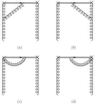
Figure 4: One-loop corrections to quasi gluon distribution, which involve one Wilson line and connects only one endpoint of internal gluon line. The double line is the Wilson line. The cross “$\times$” denotes the non-local vertex from the operator structure of definition.

We come to the diagrams which involve one Wilson line shown in Figs. 4 and 5. In Fig. 4, only one end of the internal gluon line is connected to the Wilson line, while both the ends of internal gluon line are connected to the Wilson line in Fig. 5. A direct calculation shows that

$$x\tilde{f}_{g/g}^{(1)}(x,P^{z},\Lambda)\bigg{|}_{\mathrm{Fig}.\ref{fig:wl1}(a)}=\frac{\alpha_{s}C_{A}}{4\pi}\left\{\begin{aligned} &\bigg{[}\frac{x(x+1)}{1-x}\ln\frac{x}{x-1}+\frac{1-2x}{1-x}+\frac{\Lambda}{(1-x)P^{z}}\bigg{]}_{\varoplus},&x>1\\ &\bigg{[}-\frac{x(x+1)}{1-x}\ln\frac{m^{2}_{g}(1-x+x^{2})}{4x(1-x)(P^{z})^{2}}-\frac{2x^{2}-2x+1}{1-x}+\frac{\Lambda}{(1-x)P^{z}}\bigg{]}_{+},&0<x<1\\ &\bigg{[}-\frac{x(x+1)}{1-x}\ln\frac{x}{x-1}-\frac{1-2x}{1-x}+\frac{\Lambda}{(1-x)P^{z}}\bigg{]}_{\varominus},&x<0\end{aligned}\right.$$ (20)

$$x\tilde{f}_{g/g}^{(1)}(x,P^{z},\Lambda)\bigg{|}_{\mathrm{Fig}.\ref{fig:wl1}(b)}=x\tilde{f}_{g/g}^{(1)}(x,P^{z},\Lambda)\bigg{|}_{\mathrm{Fig}.\ref{fig:wl1}(a)},$$ (21)

and

$$x\tilde{f}_{g/g}^{(1)}(x,P^{z},\Lambda)\bigg{|}_{\mathrm{Fig}.\ref{fig:wl1}(c)}=x\tilde{f}_{g/g}^{(1)}(x,P^{z},\Lambda)\bigg{|}_{\mathrm{Fig}.\ref{fig:wl1}(d)}=\frac{\alpha_{s}C_{A}}{2\pi}\left\{\begin{aligned} &\bigg{[}-1-\frac{\Lambda}{(1-x)P^{z}}\bigg{]}_{\varoplus},~{}~{}~{}~{}&x>1\\ &\bigg{[}1-\frac{\Lambda}{(1-x)P^{z}}\bigg{]}_{+},~{}~{}~{}~{}&0<x<1\\ &\bigg{[}1-\frac{\Lambda}{(1-x)P^{z}}\bigg{]}_{\varominus}.~{}~{}~{}~{}&x<0\end{aligned}\right.$$ (22)

In the above expressions, three generalized functions are introduced to regulate the singular integral Stewart:2017tvs :

$$\int^{\infty}_{1}dx~{}[f(x)]_{\varoplus}T(x) =\int^{\infty}_{1}dx~{}f(x)\left[T(x)-T(1)\right],$$ (23)

$$\int^{1}_{0}dx~{}[f(x)]_{+}T(x) =\int^{1}_{0}dx~{}f(x)\left[T(x)-T(1)\right],$$ (24)

$$\int^{0}_{-\infty}dx~{}[f(x)]_{\varominus}T(x) =\int^{0}_{-\infty}dx~{}f(x)\left[T(x)-T(1)\right].$$ (25)

Here $T(x)$ is an arbitrary smooth function. Then, the total contribution from Fig. 4 is given as

$$x\tilde{f}_{g/g}^{(1)}(x,P^{z},\Lambda)\bigg{|}_{\mathrm{Fig}.\ref{fig:wl1}}=\frac{\alpha_{s}C_{A}}{2\pi}\left\{\begin{aligned} &\bigg{[}\frac{x(1+x)}{1-x}\ln\frac{x}{x-1}-\frac{1}{1-x}-\frac{\Lambda}{(1-x)P^{z}}\bigg{]}_{\varoplus},~{}~{}~{}~{}&x>1\\ &\bigg{[}-\frac{x(1+x)}{1-x}\ln\frac{(1-x+x^{2})m^{2}_{g}}{4x(1-x)(P^{z})^{2}}+\frac{1-2x^{2}}{1-x}-\frac{\Lambda}{(1-x)P^{z}}\bigg{]}_{+},~{}~{}~{}~{}&0<x<1\\ &\bigg{[}-\frac{x(1+x)}{1-x}\ln\frac{x}{x-1}+\frac{1}{1-x}-\frac{\Lambda}{(1-x)P^{z}}\bigg{]}_{\varominus}.~{}~{}~{}~{}&x<0\end{aligned}\right.$$ (26)

One can find that the linear divergences do not vanish.

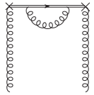
Figure 5: One-loop correction to quasi gluon distributions, which involves one Wilson line and both the endpoints of internal gluon line connect to the Wilson line. The double line is the Wilson line. The cross “$\times$” denotes the non-local vertex from the operator structure of definition.

At last we calculate the one-loop correction to the self energy of Wilson line, which is presented by Fig. 5. The result is

$$x\tilde{f}_{g/g}^{(1)}(x,P^{z},\Lambda)\bigg{|}_{\mathrm{Fig}.\ref{fig:wl2}}=\frac{\alpha_{s}C_{A}}{2\pi}\left\{\begin{aligned} &\bigg{[}\frac{1}{1-x}+\frac{\Lambda}{(1-x)^{2}P^{z}}\bigg{]}_{\varoplus},~{}~{}~{}~{}&x>1\\ &\bigg{[}\frac{1}{x-1}+\frac{\Lambda}{(1-x)^{2}P^{z}}\bigg{]}_{+},~{}~{}~{}~{}&0<x<1\\ &\bigg{[}\frac{1}{x-1}+\frac{\Lambda}{(1-x)^{2}P^{z}}\bigg{]}_{\varominus}.~{}~{}~{}~{}&x<0\end{aligned}\right.$$ (27)

The linear divergence in Eq. (27) has the similar structure with the linear divergence in quasi quark distribution, thus may be renormalized in the same approach.

At last we note that there are also contributions from crossed diagrams, which have been discussed in Ref. Wang:2017qyg . These contributions can be easily derived by using the property $\tilde{f}(-x)=-\tilde{f}(x)$.

IV Auxiliary field method and renormalization of linear divergences

The light-cone and quasi parton distribution functions are defined by the gauge invariant quark bi-linear or gluonium operator. A Wilson line, a path ordered exponential of a line integral over gluon field along a contour, is essential to retaining the gauge invariance. It has been known for a long time that loop corrections for Wilson line lead to power divergences Polyakov:1980ca ; Dotsenko:1979wb ; Brandt:1981kf . The power divergences can be summed to an exponential factor $\exp(-\pi/aL(c))$ where $1/a$ is the UV cut-off and $L(c)$ is the length of Wilson line. Based on this, the linear divergence in quasi quark distribution are cured Chen:2016fxx ; Ishikawa:2016znu ; Green:2017xeu , because all the power divergences in quasi quark distribution are from the Wilson line’s self energy. In gluon quasi PDF, it has been shown in Sec. III that Wilson line’s self energy is not the only source of linear divergence. Since the Wilson line is a functional of gluon field, the gluon operator and Wilson line might be entangled in loop corrections.

It is convenient to discuss gauge invariant non-local operator with the method of auxiliary field Gervais:1979fv . In this method, the non-local operator can be converted into local operators by introducing an auxiliary field. The action of the theory is given by

$$S=S_{\mathrm{QCD}}+i\int^{\lambda}_{0}\bar{\mathcal{Z}}\left(\frac{d}{d\lambda^{\prime}}+ig\dot{x}^{\mu}A^{a}_{\mu}t^{a}\right)\mathcal{Z}d\lambda^{\prime}+i\bar{\mathcal{Z}}(0)\mathcal{Z}(0),$$ (28)

where $S_{\mathrm{QCD}}$ is the action of QCD. Obviously the Wilson line can be expressed by the two point Green’s function of $\mathcal{Z}-$ field Samuel:1978iy ; Gervais:1979fv ; Arefeva:1980zd ; Dorn:1986dt

$$W(z_{1},z_{2};C)=\langle\mathcal{Z}(\lambda_{1})\bar{\mathcal{Z}}(\lambda_{2})\rangle_{\mathcal{Z}},$$ (29)

$\langle\cdots\rangle_{\mathcal{Z}}$ denotes the expectation value respect to $\mathcal{Z}$ only. Therefore, when $\mathcal{Z}$- field is integrated out in Eq. (28), all the internal $\mathcal{Z}$ line is just the Wilson line.

With the $\mathcal{Z}$ field technique, the gauge invariant non-local quark bi-linear operator is then given by Samuel:1978iy ; Gervais:1979fv ; Arefeva:1980zd ; Dorn:1986dt

$$\bar{\psi}_{i}(z_{2})W_{ij}(z_{2},z_{1};C)\psi_{j}(z_{1})=\langle(\bar{\psi}(z_{1})\mathcal{Z}(\lambda_{1}))(\bar{\mathcal{Z}}(\lambda_{2})\psi(z_{2}))\rangle_{\mathcal{Z}},$$ (30)

and the gauge invariant non-local gluonium operator is

$$G^{a}_{\mu\nu}(z_{1})W_{ab}(z_{1},z_{2};C)G^{b}_{\rho\sigma}(z_{2})=\langle\left(G^{a}_{\mu\nu}(z_{1})\mathcal{Z}_{a}(\lambda_{1})\right)\left(\bar{\mathcal{Z}}_{b}(\lambda_{2})G^{b}_{\rho\sigma}(z_{2})\right)\rangle_{\mathcal{Z}}.$$ (31)

Now the problem of renormalizing the non-local operator has been converted into the problem of renormalizing the local operators. The operator is divided into two local operators, which can be considered individually.

The operator $\Omega^{(1)}_{\mu\nu}=G^{a}_{\mu\nu}\mathcal{Z}_{a}$, which is a gauge invariant field strength tensor, may mix with other operators under renormalization. The allowed mixing operators are constrained by the gauge symmetry, or more strictly, the BRST symmetry, as well as the dimensional constraint. It has been demonstrated that the $\Omega^{(1)}_{\mu\nu}$ can only mix with two operators under renormalization Dorn:1981wa ; Dorn:1986dt

$$\Omega^{(1)}_{\mu\nu} =G^{a}_{\mu\nu}\mathcal{Z}_{a},$$ (32)

$$\Omega^{(2)}_{\mu\nu} =\Omega^{(1)}_{\mu\alpha}\frac{\dot{x}_{\alpha}\dot{x}_{\nu}}{\dot{x}^{2}}-\Omega^{(1)}_{\nu\alpha}\frac{\dot{x}_{\alpha}\dot{x}_{\mu}}{\dot{x}^{2}},$$ (33)

$$\Omega^{(3)}_{\mu\nu} =|\dot{x}|^{-2}(\dot{x}_{\mu}A^{a}_{\nu}-\dot{x}_{\nu}A_{\mu}^{a})(D\mathcal{Z})_{a},$$ (34)

with

$$(D\mathcal{Z})_{a}=\partial_{\lambda}\mathcal{Z}_{a}-gf_{abc}~{}\dot{x}\cdot A_{b}\mathcal{Z}_{c}.$$ (35)

The Hermitian adjoint of these operators are

$$\bar{\Omega}^{(1)}_{\mu\nu} =\bar{\mathcal{Z}}_{a}G^{a}_{\mu\nu},$$ (36)

$$\bar{\Omega}^{(2)}_{\mu\nu} =\bar{\Omega}^{(1)}_{\mu\alpha}\frac{\dot{x}_{\alpha}\dot{x}_{\nu}}{\dot{x}^{2}}-\bar{\Omega}^{(1)}_{\nu\alpha}\frac{\dot{x}_{\alpha}\dot{x}_{\mu}}{\dot{x}^{2}},$$ (37)

$$\bar{\Omega}^{(3)}_{\mu\nu} =(-\bar{\mathcal{Z}}\overleftarrow{D})_{a}|\dot{x}|^{-2}(\dot{x}_{\mu}A^{a}_{\nu}-\dot{x}_{\nu}A_{\mu}^{a}),$$ (38)

with

$$(\bar{\mathcal{Z}}\overleftarrow{D})_{a}=-\partial_{\lambda}\bar{\mathcal{Z}}_{a}-gf_{abc}~{}\dot{x}\cdot A_{b}\bar{\mathcal{Z}}_{c}.$$ (39)

After renormalization, the operator $\Omega^{(1)}_{\mu\nu}$ can be replaced by the operators $\Omega^{(i)(r.)}_{\mu\nu}(i=1,2,3)$ as

$$\Omega^{(1)}_{\mu\nu}\rightarrow c_{1}\Omega^{(1)(r.)}_{\mu\nu}+c_{2}\Omega^{(2)(r.)}_{\mu\nu}+c_{3}\Omega^{(3)(r.)}_{\mu\nu},$$ (40)

where the $c_{i}~{}(i=1,2,3)$ are the mixing parameters, and the superscript $(r.)$ denotes that the $\mathcal{Z}$ field in the operators are renormalized.

However, the operator we are interested in is not the gluonium operator with full Lorentz indices. In the definition of quasi gluon distribution, the operator should contract with $n_{z}$, which is the unit tangent vector of the Wilson line contour. One can easily find that $\Omega^{(1)}_{z\mu}=\Omega^{(2)}_{z\mu}$. Therefore, in the present work, $\Omega^{(1)}_{\mu\nu}$ and $\Omega^{(2)}_{\mu\nu}$ are not distinguishable.

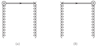
Figure 6: The tree-level counter-term contribution, where $\bigotimes$ denotes the counter-term from matrix elements of $\Omega^{(3)(r.)}_{z\mu}$ or $\bar{\Omega}^{(3)(r.)}_{z\mu}$.

To study the renormalization of operator we should calculate the tree level matrix element from the operator $\Omega^{(3)}_{\mu\nu}$. Note that the operator we are interested in is $\Omega^{(3)}_{z\mu}$. Since an arbitrary point on $W(z,0,L_{n_{z}})$ can be expressed as $x(\lambda)=\lambda zn_{z}$, we have

$$\Omega^{(3)}_{z\mu} =|\dot{x}|^{-2}(\dot{x}_{z}A^{a}_{\mu}-\dot{x}_{\mu}A^{a}_{z})(D\mathcal{Z})_{a}=-\frac{z}{|z|^{2}}A^{a}_{\mu}(D\mathcal{Z})_{a}.$$ (41)

Because the path in the Wilson line is along the $z$ direction, the $\mu$ component $(\mu=0,1,2)$ of $\dot{x}$ is zero.

Before calculating the tree-level matrix elements we make some remarks on the renormalization of $\mathcal{Z}$ field. Under renormalization, the $\mathcal{Z}$ field gets a renormalized mass $\delta m_{z}$. Therefore, after renormalization, the equation of motion for $\mathcal{Z}$ and $\bar{\mathcal{Z}}$ should be

$$\partial_{\lambda}\mathcal{Z}_{a}-gf_{abc}~{}\dot{x}\cdot A_{b}\mathcal{Z}_{c}+\delta m_{z}|z|\mathcal{Z}^{a}= 0,$$ (42)

$$\partial_{\lambda}\bar{\mathcal{Z}}_{a}+gf_{abc}~{}\dot{x}\cdot A_{b}\bar{\mathcal{Z}}_{c}-\delta m_{z}|z|\bar{\mathcal{Z}}^{a}= 0.$$ (43)

Then, the contraction of $\Omega^{(3)(r.)}_{z\mu}$ and external gluon state gives

$$\langle\vbox{\halign{#\cr\vphantom{\hrulefill}\crcr\kern 3.2pt\nointerlineskip\cr\vphantom{\hrulefill}\crcr\kern 3.2pt\nointerlineskip\cr\vphantom{\hrulefill}\crcr\nointerlineskip\cr$\hfil\textstyle{\vbox to14.0pt{}\hskip 2.56422pt}\hfil$\crcr}}\kern-0.2pt\raise 6.30554pt\hbox{\vrule height=7.89447pt,width=0.4pt}\kern-0.2pt\vbox{\halign{#\cr\vphantom{\hrulefill}\crcr\kern 3.2pt\nointerlineskip\cr\vphantom{\hrulefill}\crcr\kern 3.2pt\nointerlineskip\cr\hrulefill\crcr\nointerlineskip\cr$\hfil\textstyle{\vbox to14.0pt{}\hskip 2.56422pt}\hfil$\crcr}}\kern-2.56422pt\kern-2.56422pt\hbox{$\textstyle{g}$}\vbox{\halign{#\cr\vphantom{\hrulefill}\crcr\kern 3.2pt\nointerlineskip\cr\vphantom{\hrulefill}\crcr\kern 3.2pt\nointerlineskip\cr\hrulefill\crcr\nointerlineskip\cr$\hfil\textstyle{\vbox to14.0pt{}(p)|}\hfil$\crcr}}\vbox{\halign{#\cr\vphantom{\hrulefill}\crcr\kern 3.2pt\nointerlineskip\cr\vphantom{\hrulefill}\crcr\kern 3.2pt\nointerlineskip\cr\hrulefill\crcr\nointerlineskip\cr$\hfil\textstyle{\vbox to14.0pt{}\hskip 3.61111pt}\hfil$\crcr}}\kern-0.2pt\raise 8.83331pt\hbox{\vrule height=5.3667pt,width=0.4pt}\kern-0.2pt\vbox{\halign{#\cr\vphantom{\hrulefill}\crcr\kern 3.2pt\nointerlineskip\cr\vphantom{\hrulefill}\crcr\kern 3.2pt\nointerlineskip\cr\vphantom{\hrulefill}\crcr\nointerlineskip\cr$\hfil\textstyle{\vbox to14.0pt{}\hskip 3.61111pt}\hfil$\crcr}}\kern-3.61111pt\kern-3.61111pt\hbox{$\textstyle{\Omega}$}^{(3)(r.)}_{z\mu}(z^{\prime})=-\epsilon^{*}_{\mu}(p)e^{ip\cdot z^{\prime}}\frac{z}{|z|^{2}}(D\mathcal{Z})_{a}=\delta m_{z}\frac{z}{|z|}\epsilon^{*}_{\mu}(p)e^{ip\cdot z^{\prime}}\mathcal{Z}_{a},$$ (64)

where the equation of motion for $\mathcal{Z}$ (Eq. (43)) is used.

The contributions from $\Omega^{(3)(r.)}_{z\mu}$ at tree level are shown in Fig. 6. For Fig. 6(a), with the contraction rule presented in Eq. (64), its contribution to quasi gluon distribution reads

$$x\tilde{f}_{g/g}(x,P^{z},\Lambda)\bigg{|}_{\mathrm{Fig.}\ref{fig:cterm1}(a)}= \int\frac{dz}{2\pi P^{z}}e^{ixP^{z}z}\langle g(p)|\langle(G^{z}_{~{}\mu}\mathcal{Z})(zn_{z})\bar{\Omega}^{(3)(r.)\mu z}(0)\rangle_{\mathcal{Z}}|g(p)\rangle^{(0)}$$

$$= \frac{1}{2(N^{2}_{c}-1)}\delta^{aa^{\prime}}\sum_{i}\epsilon_{\mu,i}(p)\epsilon^{*\mu}_{i}(p)\int\frac{dz}{2\pi P^{z}}e^{ixP^{z}z}iP^{z}e^{-iP^{z}z}(\delta m_{z})\frac{-z}{|z|}\langle\mathcal{Z}_{a}(1)\bar{\mathcal{Z}}_{a^{\prime}}(0)\rangle_{\mathcal{Z}}$$

$$= iP^{z}\delta m_{z}\int\frac{dz}{2\pi P^{z}}e^{i(x-1)P^{z}z}\lim_{\epsilon\to 0}\frac{z}{|z|}e^{-\epsilon|z|}$$

$$= iP^{z}\delta m_{z}\int\frac{dz}{2\pi P^{z}}e^{i(x-1)P^{z}z}\lim_{\epsilon\to 0}\int^{\infty}_{0}d\alpha\frac{ze^{-\alpha\epsilon^{2}-\frac{z^{2}}{4\alpha}}}{2\sqrt{\pi}\alpha^{\frac{3}{2}}}$$

$$= iP^{z}\delta m_{z}\int\frac{dz}{2\pi P^{z}}e^{i(x-1)P^{z}z}\lim_{\epsilon\to 0}\int^{\infty}_{0}d\alpha\int^{+\infty}_{-\infty}dk^{z}\frac{k^{z}}{i\pi}e^{-\alpha((k^{z})^{2}+\epsilon^{2})}(1-e^{-ik^{z}z})$$

$$= P^{z}\delta m_{z}\int\frac{dz}{2\pi P^{z}}e^{i(x-1)P^{z}z}\lim_{\epsilon\to 0}\int^{+\infty}_{-\infty}\frac{dk^{z}}{\pi}\frac{k^{z}}{(k^{z})^{2}+\epsilon^{2}}(1-e^{-ik^{z}z})$$

$$= \delta m_{z}\int^{+\infty}_{-\infty}\frac{dk^{z}}{\pi}\frac{\delta((x-1)P^{z})-\delta((x-1)P^{z}-k^{z})}{k^{z}}$$

$$= \frac{\delta m_{z}}{\pi P^{z}}\left[\frac{1}{1-x}-\delta(1-x)\int dy\frac{1}{1-y}\right]$$

$$= \frac{\delta m_{z}}{\pi P^{z}}\left\{\begin{aligned} &\left[\frac{1}{1-x}\right]_{\varoplus},&x>1\\ &\left[\frac{1}{1-x}\right]_{+},&0<x<1\\ &\left[\frac{1}{1-x}\right]_{\varominus}.&x<0\end{aligned}\right.$$ (65)

Here the superscript $(0)$ denotes the tree level matrix element. In the above expression, $\langle\mathcal{Z}_{a}\bar{\mathcal{Z}}_{a^{\prime}}\rangle_{\mathcal{Z}}$ is taken to be $\delta_{aa^{\prime}}$ by recalling Eq. (29) and also the fact that the matrix element is at tree level. It is interesting to notice that the divergence has the same structure with Eq. (26). Fig. 6(b) gives the same contribution. Thus we have

$$x\tilde{f}_{g/g}(x,P^{z},\Lambda)\bigg{|}_{\mathrm{Fig.}\ref{fig:cterm1}}=\frac{2\delta m_{z}}{\pi}\left\{\begin{aligned} &\left[\frac{1}{1-x}\right]_{\varoplus},&x>1\\ &\left[\frac{1}{1-x}\right]_{+},&0<x<1\\ &\left[\frac{1}{1-x}\right]_{\varominus}.&x<0\end{aligned}\right.$$ (66)

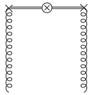
Figure 7: The tree-level counter-term contribution, where $\bigotimes$ denotes the mass counter-term of the Wilson line.

Now we calculate the contribution from Fig. 7. For a Wilson line in fundamental representation, it has been shown that Polyakov:1980ca ; Dotsenko:1979wb ; Brandt:1981kf

$$W(z_{1},z_{2};C)^{(r.)}=Z^{-1}\exp\left(-\delta m_{z}\|C(\lambda_{1},\lambda_{2})\|\right)W(z_{1},z_{2};C),$$ (67)

where $\|C\|$ denotes the length of the contour $C$. $Z$ is a renormalization constant. Similarly, for a Wilson line $W(z,0,L_{n^{z}})$ in the adjoint representation, we have

$$W(zn_{z},0;L_{n_{z}})^{(r.)} =e^{-\delta m_{z}|z|}W(zn_{z},0;L_{n_{z}})$$

$$=1-\delta m_{z}|z|+W^{(1)}(zn_{z},0;L_{n_{z}})+\cdots.$$ (68)

Therefore, with the same trick in Ref. Chen:2016fxx , the leading order contribution from the counter term reads

$$\int\frac{dz}{2\pi P^{z}}e^{ixP^{z}z}(-\delta m_{z}|z|)\langle g(p)|G^{z}_{~{}\mu}(zn_{z})G^{\mu z}(0)|g(p)\rangle^{(0)}$$

$$= (-\delta m_{z})\int\frac{dz}{2\pi P^{z}}e^{ixP^{z}z}|z|(P^{z})^{2}e^{-izP^{z}}$$

$$= (-\delta m_{z})P^{z}\int\frac{dz}{2\pi}e^{i(x-1)P^{z}z}|z|$$

$$= -\delta m_{z}P^{z}\int\frac{dk^{z}}{\pi}\frac{\delta((1-x)P^{z})-\delta(k^{z}-(1-x)P^{z})}{(k^{z})^{2}}$$

$$= -\frac{\delta m_{z}}{\pi P^{z}}\left[-\frac{1}{(1-x)^{2}}+\delta(1-x)\int dy\frac{1}{(1-y)^{2}}\right]$$

$$= \frac{\delta m_{z}}{\pi P^{z}}\left\{\begin{aligned} &\left[\frac{1}{(1-x)^{2}}\right]_{\varoplus},&x>1\\ &\left[\frac{1}{(1-x)^{2}}\right]_{+},&0<x<1\\ &\left[\frac{1}{(1-x)^{2}}\right]_{\varominus}.&x<0\end{aligned}\right.$$ (69)

Now we turn back to the one-loop corrections, shown by Figs. 4 and 5. Fig. 5 denotes the self-energy of Wilson line, and the linear divergence in this diagram should be canceled by the one in Fig. 7. From Eqs. (27) and (69), one can determine that

$$\delta m_{z}=-\frac{\alpha_{s}C_{A}}{2\pi}(\pi\Lambda).$$ (70)

Fig. 4 is the one-loop correction to the gluon-Wilson line vertex. In the language of $\mathcal{Z}$ field formalism, it can also been interpreted as the one-loop corrections to $\Omega^{(1)}_{z\mu}$. The linear divergence in Fig. 4 should be canceled by the one in Fig. 6. From Eqs. (26) and (65) one can find that the structures of linear divergences are identically the same. It indicates that all these linear divergences can be renormalized by operator $\Omega^{(3)(r.)}_{z\mu}$, with only the mixing parameter $c_{3}$ undetermined. From Eq. (70) and Eq. (26), we have $c_{3}=-1/2$. Then, at one-loop level, all the linear divergences in quasi gluon distribution can be absorbed by $\delta m_{z}$, and the matrix elements of $\Omega^{(3)(r.)}_{z\mu}$.

The above calculation has been performed in the “naive” cut-off scheme, which may break the gauge symmetry at first sight. A complete analysis relies on the lattice perturbation theory. But it is viable to examine the gauge invariance from another viewpoint. In Ref. Wang:2017qyg , we have calculated the matching coefficient in the dimensional regularization scheme. It is interesting to notice that the differences between the cut-off and DR schemes only reside in the linearly divergent terms, while the finite terms are the same. It is widely believed that gauge invariance is preserved in DR. In the present work, the linearly divergent terms have been absorbed into the matrix elements of the gauge invariant operators, leaving the finite terms consistent with the DR. Therefore, it is likely that our results are gauge invariant.

To further validate the above proposal, one needs to investigate the cancelation of linear divergences for all loops. A complete proof is left for a future study, and here we outline the proof at two-loop level. Higher order corrections can be generated by adding internal lines step by step from lower order diagrams. The contribution from a $n$-loop diagram with $k$ propagators can be generally written as

$$\int d^{4}l_{1}d^{4}l_{2}\cdots d^{4}l_{n}\frac{N_{1}N_{2}\cdots N_{j}}{D_{1}D_{2}\cdots D_{k}}\delta\left(\sum_{i=1}^{n}c_{i}l^{z}_{i}-(1-x)P^{z}\right)$$

$$= \int dl^{z}_{1}dl^{z}_{2}\cdots dl^{z}_{n}\delta\left(\sum_{i=1}^{n}c_{i}l^{z}_{i}-(1-x)P^{z}\right)\left[\int d^{3}l_{1}d^{3}l_{2}\cdots d^{3}l_{n}\frac{N_{1}N_{2}\cdots N_{j}}{D_{1}D_{2}\cdots D_{k}}\right],$$ (71)

with $d^{3}l_{i}\equiv dl^{0}_{i}d^{2}l_{i\perp}$. Here $N_{i}$ and $D_{i}$ denote the numerator and denominator respectively, and $c_{i}$ are some constants. In the discussions of Sec. III and Sec. IV, the $z$ component of loop momentum is either constrained by the $\delta$ function, or left unintegrated. It has been shown that the linear divergences come from the integration over the “0” and transverse components of loop momenta. Therefore, we separate the $z$-components of the loop momenta $l_{i}$ and leave them unintegrated. Then the loop integrals in the bracket […] are all three-dimensional (3D) integrals. We define a few quantities for a general diagram as follows:

• $L$: The number of loops.

• $F$: The number of internal fermions.

• $G$: The number of internal gluons and ghosts.

• $V_{3g}$: The number of three-gluon vertices and gluon-ghost vertices.

• $V_{G}$: The number of vertices corresponding to the Abelian part of field strength tensor. In addition, no external line should connects to these vertices.

With these quantities, we introduce the superficial degree of divergence $D$ for the 3D integrals, with $D=3L-F-2G+V_{3g}+V_{G}$. The propagator of Wilson line only involves the $z$-component of momentum, hence will not affect the 3D superficial degree of divergence.

There are three generic ways to generate two-loop diagrams from the one-loop diagram.

• None of the added internal line touches the Wilson line, which are shown in Fig. 8. This is the same with ordinary Feynman diagrams in QCD. For Fig. 8(a, b), adding one gluon line will introduce two three-gluon vertices and three gluon propagators, i.e., $G\to G+3$, $V_{3g}\to V_{3g}+2$ and $L\to L+1$. In this case $D$ will be decreased by 1. A linear divergence will reduce to a logarithm divergence, so there is no need to further subtract the linear divergence. Fig. 8(c) contains gluon’s self energy, although $D$ is increased by 1, the power divergence must be canceled by additional diagrams due to the gauge invariance, which has been discussed at the beginning of Sec. III.

  

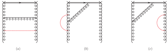
  Figure 8: Typical two-loops corrections to quasi gluon distribution, in which the added internal line (denoted by dotted line) is not connected to the Wilson line.

• Only one endpoint of the added gluon line is attached to Wilson line. This is shown in Fig. 9. For Fig. 9(a), there will be two more gluon propagators, one three-gluon vertex, and one Wilson line propagator, i.e., $G\to G+2$, $V_{3g}\to V_{3g}+1$, and $L\to L+1$, then $D$ will not be modified; For Fig. 9(b), there will be two more gluon propagators, one three-gluon vertex, and one Wilson line propagator as well, but $V_{G}$ will be modified from 1 to 2, then $D$ will be increased by 1. The power divergence in this diagram can be viewed as the product of two linear divergences, which are from the one-loop corrections of the gluon-Wilson line (or gluon-$\mathcal{Z}$) vertices. In this case, the power divergence can be removed by adding contributions from $\Omega^{(3)(r.)}_{\mu\nu}$. For Fig. 9(a) just one counter term is needed, while for (b) we need two counter terms.

  

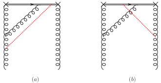
  Figure 9: Typical two-loops corrections to quasi gluon distribution, in which only one endpoint of the added internal gluon line is connected to the Wilson line.

• Both the endpoints of the added gluon line touch the Wilson line, which are shown in Fig. 10. In this case there will be one more gluon propagator, i.e., $G\to G+1$, and two more Wilson line propagators, then $D$ will be increased by 1. This case can be explained as Wilson line’s self energy. The power divergence for this case should be cured by adding mass counter term $\delta m_{z}$ of the Wilson line, as well as the corresponding counter term for the linear divergence from the lower order diagram.

  

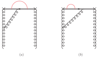
  Figure 10: Typical two-loops corrections to quasi gluon distribution, in which both the endpoints of the added gluon line are connected to the Wilson line.

The above discussions on two-loop corrections are conjectured to hold to all orders, though we are lack of a complete all-order proof.

After discussing the linear divergence we add some remarks on the logarithm divergence. From Sec. III one can find that there is no logarithm divergence in the one-loop real corrections. By employing the auxiliary field approach the renormalization of gauge invariant quark bi-linear and gluonium operators has been discussed in DR scheme for a long time Craigie:1980qs ; Dorn:1981wa ; Dorn:1986dt . Note that in DR the linear divergence is not regularized. A remarkable simplification is achieved when the gluonium operator is contracted with the tangents of the contour, in this case, the operator will not be renormalized Dorn:1981wa ; Dorn:1986dt , i.e.,

$$\dot{x}_{\mu}G^{\mu\nu\rho\sigma}\dot{x}_{\sigma}=\dot{x}_{\mu}(G^{\mu\nu\rho\sigma})^{(r.)}\dot{x}_{\sigma}$$ (72)

with

$$G^{\mu\nu\rho\sigma}=G^{\mu\nu}(z_{1})W(z_{1},z_{2};C)G^{\rho\sigma}(z_{2}).$$ (73)

This can be traced back to the property of functional derivation of Wilson line. The quasi gluon distribution belongs to this case.

It is also shown that the quasi distributions can be defined from other components of the correlators. For example, the quasi quark distribution can be defined by the matrix element of $\bar{\psi}(z)\gamma^{0}\psi(0)$ Xiong:2013bka . For gluon, one can pick up any indices of ${\mu}$ and $\nu$ in the matrix elements of $G^{\mu\rho}(z)W(z,0,L_{n_{z}})G_{\rho}^{~{}\nu}(0)$, in present work we choose $\mu=\nu=z$. Eq. (72) indicates that, if one defines quasi gluon distribution by specifying $\mu$ and $\nu$ components of gluonium operator, the renormalization of logarithm divergence will be greatly simplified when the tangents of the contour are collinear to the projection vector corresponding to these components; On the other hand, if one modifies the contour of the Wilson line (e.g., in the non-dipolar Wilson line approach Li:2016amo ), it is more convenient to modify the components of gluon strength tensor correspondingly.

V Matching coefficient for improved gluon distribution

With the discussions in Sec. IV, we propose the subtracted quasi gluon distribution as

$$x\tilde{f}^{(r.)}_{g/H}(x,P^{z},\Lambda)=\int\frac{dz}{2\pi P^{z}}e^{ixzP^{z}}\bigg{\langle}P\bigg{|}\bigg{\langle}\left(\Omega^{(1)(r.)z}_{~{}~{}~{}~{}~{}~{}~{}\mu}+c_{3}\Omega^{(3)(r.)z}_{~{}~{}~{}~{}~{}~{}~{}\mu}\right)(zn_{z})\left(\bar{\Omega}^{(1)(r.)\mu z}+c_{3}\bar{\Omega}^{(3)(r.)\mu z}\right)(0)\bigg{\rangle}_{\mathcal{Z}}\bigg{|}P\bigg{\rangle},$$ (74)

where $c_{3}=-1/2+O(\alpha_{s})$ is the mixing parameter determined by perturbation theory. $\delta m_{z}$ and the matrix elements can be evaluated non-perturbatively in LQCD. According to LaMET, one can expect a factorization formula as

$$x\tilde{f}^{(r.)}_{g/H}(x,P^{z},\Lambda)=\int^{1}_{0}\frac{dy}{y}Z_{gi}\left(\frac{x}{y},\frac{\Lambda}{P^{z}}\right)yf_{i/H}(y,\Lambda).$$ (75)

In perturbation theory the $Z_{gg}$ can be expanded as

$$Z_{gg}\left(\xi,\frac{\Lambda}{P^{z}}\right)=\sum_{i=0}^{\infty}\left(\frac{\alpha_{s}}{2\pi}\right)^{n}Z^{(n)}_{gg}\left(\xi,\frac{\Lambda}{P^{z}}\right),$$ (76)

with $Z^{(0)}_{gg}(\xi)=\delta(1-\xi)$, $\xi\equiv x/y$.

The one-loop correction to light-cone gluon distribution has already been calculated in Ref. Wang:2017qyg , with result

$$xf_{g/g}^{(1)}(x,\Lambda)\bigg{|}_{\mathrm{total}.}= \frac{\alpha_{s}C_{A}}{2\pi}\bigg{\{}\bigg{[}(2x^{3}-3x^{2}+2x-2)\ln\frac{(1-x+x^{2})m^{2}_{g}}{\Lambda^{2}}-\frac{3x}{2(1-x+x^{2})}+2x^{2}(x-1)+\frac{7}{2}x-2\bigg{]}$$

$$-\frac{x^{2}(1+x)}{1-x}\ln\frac{(1-x+x^{2})m^{2}_{g}}{\Lambda^{2}}-\delta(1-x)\int^{1}_{0}dy\frac{1+y}{1-y}\ln\frac{\Lambda^{2}}{(1-y+y^{2})m^{2}_{g}}\bigg{\}}$$

$$= \frac{\alpha_{s}C_{A}}{2\pi}\bigg{\{}(2x^{3}-2x^{2}+4x-1)\ln\frac{(1-x+x^{2})m^{2}_{g}}{\Lambda^{2}}+\bigg{[}\frac{x+1}{x-1}\ln\frac{(1-x+x^{2})m^{2}_{g}}{\Lambda^{2}}\bigg{]}_{+}$$

$$+2x^{2}(x-1)+\frac{7}{2}x-2-\frac{3x}{2(1-x+x^{2})}\bigg{\}}$$ (77)

for $0<x<1$. The result is 0 for $x>1$ and $x<0$. On the other hand, the one-loop correction to gluon-in-gluon quasi distribution reads

$$x\tilde{f}_{g/g}^{(r.)(1)}(x,P^{z},\Lambda)\bigg{|}_{total.}=\frac{\alpha_{s}C_{A}}{2\pi}\left\{\begin{aligned} &(2x^{3}-2x^{2}+4x-1)\ln\frac{x-1}{x}+\bigg{[}\frac{x+1}{x-1}\ln\frac{x-1}{x}\bigg{]}_{\varoplus}\\ &+2x^{2}-2x+3,~{}~{}~{}~{}&x>1\\ &(2x^{3}-2x^{2}+4x-1)\ln\frac{(1-x+x^{2})m^{2}_{g}}{4x(1-x)(P^{z})^{2}}\\ &+\bigg{[}\frac{x+1}{x-1}\ln\frac{(1-x+x^{2})m^{2}_{g}}{4x(1-x)(P^{z})^{2}}+\frac{2x^{2}}{x-1}\bigg{]}_{+}\\ &+\frac{8x^{5}-12x^{4}+21x^{3}-15x^{2}+8x-2}{2\left(1-x+x^{2}\right)},~{}~{}~{}~{}&0<x<1\\ &-(2x^{3}-2x^{2}+4x-1)\ln\frac{x-1}{x}-\bigg{[}\frac{x+1}{x-1}\ln\frac{x-1}{x}\bigg{]}_{\varominus}\\ &-2x^{2}+2x-3.~{}~{}~{}~{}&x<0\end{aligned}\right.$$ (78)

From Eqs. (V) and (78), one can determine the matching coefficient at one-loop level,

$$Z^{(1)}_{gg}\bigg{(}\xi,\frac{\Lambda}{P^{z}}\bigg{)}=C_{A}\left\{\begin{aligned} &(2\xi^{3}-2\xi^{2}+4\xi-1)\ln\frac{\xi-1}{\xi}+\bigg{[}\frac{\xi+1}{\xi-1}\ln\frac{\xi-1}{\xi}\bigg{]}_{\varoplus}+2\xi^{2}-2\xi+3,~{}~{}~{}~{}&\xi>1\\ &(2\xi^{3}-2\xi^{2}+4\xi-1)\ln\frac{\Lambda^{2}}{4\xi(1-\xi)(P^{z})^{2}}+\bigg{[}\frac{\xi+1}{\xi-1}\ln\frac{\Lambda^{2}}{4\xi(1-\xi)(P^{z})^{2}}\bigg{]}_{+}\\ &+\bigg{[}\frac{2\xi^{2}}{\xi-1}\bigg{]}_{+}+2\xi^{3}+\xi+1,~{}~{}~{}~{}&0<\xi<1\\ &-(2\xi^{3}-2\xi^{2}+4\xi-1)\ln\frac{\xi-1}{\xi}-\bigg{[}\frac{\xi+1}{\xi-1}\ln\frac{\xi-1}{\xi}\bigg{]}_{\varominus}-2\xi^{2}+2\xi-3.~{}~{}~{}~{}&\xi<0\end{aligned}\right.$$ (79)

This coefficient has only the logarithmic dependent on the cut-off $\Lambda$. It is free of IR divergence, which indicates that the LaMET factorization holds for gluon distribution at one-loop level.

VI summary and outlook

In this work we have discussed power divergences in the quasi gluon distribution. The gluon PDF is parametrized by two gluon field strength tensors contracted with each other. From the viewpoint of covariance, we proposed in the contraction to sum all components of Lorentz indices instead of only transverse ones. With this definition, we have re-calculated the gluon-in-gluon quasi distribution function at one-loop level, in which the Abelian and non-Abelian contributions are separated.

We found that power divergences cancel in diagrams without Wilson line, and not all linear divergences can be attributed into the renormalization of Wilson line. Employing auxiliary field method, we express the Wilson line as the expectation value of the product of two auxiliary fields. We found that a new operator can mix with the gauge invariant gluon field strength tensor, and pointed out that the power divergence can be absorbed into the matrix elements of this newly introduced operator at one-loop level. This cancelation of power divergence is conjectured to hold to all orders.

We note that since one can identify the $\mathcal{Z}$ field as a Wilson line $\mathcal{Z}(z)=W(z,\infty,L_{n_{z}})$, this new operator is a product of covariant derivatives of Wilson line. We then have used an improved quasi gluon distribution, and determined the matching coefficient at one-loop level. This matching coefficient is IR finite and free of UV power divergence. Therefore, the present work provides the possibility of extracting gluon distributions from LaMET and LQCD calculation.

We have to note that it is still a challenge of evaluating gluon PDF on the lattice and the present work leaves substantial room for improvement.

• In this work, we only consider the quasi gluon PDF in continuum QCD, the non-local gluon operators are constructed by the gluon field strength tensor and Wilson lines are under adjoint representation. To simulate quasi gluon PDF on the lattice, one should define quasi PDF and perform the matching calculation in lattice gauge theory, in which the gauge field is expressed by the Wilson loops under fundamental representation. For a practical lattice evaluation, one needs to define the gauge invariant non-local gluon operators by the renormalized Wilson loops under fundamental representation. The mixing of the gauge invariant gluon operators should be considered as well.

• Since the quasi PDF should be evaluated on the lattice while the light-cone PDF is defined in continuum, one has to match the light-cone PDF in continuum to the quasi PDF calculated with the lattice regularization. Furthermore, to arrive at a reliable result, renormalizing the matrix elements on the lattice is also a crucial step. Two approaches have been employed to renormalize the quasi quark PDF, one is the lattice perturbation theory Chen:2016fxx ; Carlson:2017gpk ; Xiong:2017jtn ; Constantinou:2017sej , another one is the nonperturbative renormalization approach, e.g., the RI/MOM scheme Alexandrou:2017huk ; Chen:2017mzz ; Lin:2017ani ; Green:2017xeu ; Stewart:2017tvs . The renormalized matrix element in RI/MOM is independent of UV regularization, thus one can match the lattice evaluated quasi PDF to the $\overline{\mathrm{MS}}$ renormalized light-cone PDF, and work out the matching coefficient in DR, instead of the naive cut-off. However, applying RI/MOM to gluon operators is not straightforward for quasi gluon PDF, the reason is that the multiplicative renormalizability is not clear for non-local gluon operator, during to the operator mixing discussed in this paper. At the moment, a perturbative renormalization with lattice perturbation theory will be useful in practical extraction of gluon PDF.

These issues will be addressed in the forthcoming work.

Appendix A Cancelation of the linear divergences in no-Wilson line diagrams

In Sec. III, we have concluded that the linear divergences cancel between the diagrams which with no Wilson line (Fig. 3). In the following discussion, we will show that how the cancelation works.

The UV divergence appears when loop momenta go to infinity. Since the $z$ component of loop momentum in one-loop real correction is constrained by the $\delta$ function, the UV divergence is from the region $k\sim(\Lambda,\Lambda,\Lambda,P^{z})$, where $k$ is the loop momentum and $\Lambda\gg P^{z}$ is the largest scale. In this region, one can neglect $k^{z}$ as well as the external momentum $P$. Then, under this approximation, $k$ is replaced by $\tilde{k}=(k^{0},k^{x},k^{y},0)$. To compare with the original definition in Refs. Ji:2013dva ; Ma:2017pxb ; Wang:2017qyg and the new definition in Eq. (4), we calculate the correlation matrix element

$$\mathcal{M}^{\mu\nu}=\int\frac{dz}{2\pi P^{z}}e^{ixzP^{z}}\langle g(P)|G^{z\mu}(zn_{z})G^{\nu z}(0)|g(P)\rangle.$$ (80)

Since we are interested in the no-Wilson diagrams, the Wilson line has been eliminated.

In the region $k\sim(\Lambda,\Lambda,\Lambda,P^{z})$, for Fig. 3, we have

$$\mathcal{M}^{\mu\nu}\bigg{|}_{\mathrm{Fig.}\ref{fig:nowl}(a)} \sim-2ig^{2}C_{A}\frac{n^{2}}{P^{z}}\int\frac{d^{3}\tilde{k}}{(2\pi)^{4}}\frac{\tilde{k}^{\mu}\tilde{k}^{\nu}k^{2}_{\perp}}{(\tilde{k}^{2})^{3}}+O(\Lambda^{0}),$$ (81)

$$\mathcal{M}^{\mu\nu}\bigg{|}_{\mathrm{Fig.}\ref{fig:nowl}(b)} \sim ig^{2}C_{A}\frac{n^{2}}{P^{z}}\int\frac{d^{3}\tilde{k}}{(2\pi)^{4}}\frac{k^{\mu}_{\perp}\tilde{k}^{\nu}}{(\tilde{k}^{2})^{2}}+O(\Lambda^{0}),$$ (82)

$$\mathcal{M}^{\mu\nu}\bigg{|}_{\mathrm{Fig.}\ref{fig:nowl}(c)} \sim ig^{2}C_{A}\frac{n^{2}}{P^{z}}\int\frac{d^{3}\tilde{k}}{(2\pi)^{4}}\frac{\tilde{k}^{\mu}k^{\nu}_{\perp}}{(\tilde{k}^{2})^{2}}+O(\Lambda^{0}),$$ (83)

$$\mathcal{M}^{\mu\nu}\bigg{|}_{\mathrm{Fig.}\ref{fig:nowl}(d)} \sim-ig^{2}C_{A}\frac{n^{2}}{2P^{z}}\int\frac{d^{3}\tilde{k}}{(2\pi)^{4}}\frac{g^{\mu\nu}_{\perp}}{\tilde{k}^{2}}+O(\Lambda^{0}),$$ (84)

$$\mathcal{M}^{\mu\nu}\bigg{|}_{\mathrm{Fig.}\ref{fig:nowl}(e)} \sim ig^{2}C_{A}\frac{n^{2}}{P^{z}}\int\frac{d^{3}\tilde{k}}{(2\pi)^{4}}\frac{\tilde{k}^{\mu}\tilde{k}^{\nu}}{(\tilde{k}^{2})^{2}}+O(\Lambda^{0}).$$ (85)

By contracting $\mathcal{M}^{\mu\nu}$ with $g_{\mu\nu}$ we arrive at the definition of quasi gluon PDF adopted in this work. Then, from the above results, we have

$$x\tilde{f}(x,P^{z},\Lambda)\bigg{|}_{\mathrm{Fig.}\ref{fig:nowl}(a)} \sim-2ig^{2}C_{A}\frac{n^{2}}{P^{z}}\int\frac{d^{3}\tilde{k}}{(2\pi)^{4}}\frac{k^{2}_{\perp}}{(\tilde{k}^{2})^{2}}+O(\Lambda^{0}),$$ (86)

$$x\tilde{f}(x,P^{z},\Lambda)\bigg{|}_{\mathrm{Fig.}\ref{fig:nowl}(b)} \sim ig^{2}C_{A}\frac{n^{2}}{P^{z}}\int\frac{d^{3}\tilde{k}}{(2\pi)^{4}}\frac{k^{2}_{\perp}}{(\tilde{k}^{2})^{2}}+O(\Lambda^{0}),$$ (87)

$$x\tilde{f}(x,P^{z},\Lambda)\bigg{|}_{\mathrm{Fig.}\ref{fig:nowl}(c)} \sim ig^{2}C_{A}\frac{n^{2}}{P^{z}}\int\frac{d^{3}\tilde{k}}{(2\pi)^{4}}\frac{k^{2}_{\perp}}{(\tilde{k}^{2})^{2}}+O(\Lambda^{0}),$$ (88)

$$x\tilde{f}(x,P^{z},\Lambda)\bigg{|}_{\mathrm{Fig.}\ref{fig:nowl}(d)} \sim-ig^{2}C_{A}\frac{n^{2}}{P^{z}}\int\frac{d^{3}\tilde{k}}{(2\pi)^{4}}\frac{1}{\tilde{k}^{2}}+O(\Lambda^{0}),$$ (89)

$$x\tilde{f}(x,P^{z},\Lambda)\bigg{|}_{\mathrm{Fig.}\ref{fig:nowl}(e)} \sim ig^{2}C_{A}\frac{n^{2}}{P^{z}}\int\frac{d^{3}\tilde{k}}{(2\pi)^{4}}\frac{1}{\tilde{k}^{2}}+O(\Lambda^{0}).$$ (90)

One can find that in the region $k\sim(\Lambda,\Lambda,\Lambda,P^{z})$,

$$x\tilde{f}(x,P^{z},\Lambda)\bigg{|}_{\mathrm{Fig.}\ref{fig:nowl}(a)}+x\tilde{f}(x,P^{z},\Lambda)\bigg{|}_{\mathrm{Fig.}\ref{fig:nowl}(b)}+x\tilde{f}(x,P^{z},\Lambda)\bigg{|}_{\mathrm{Fig.}\ref{fig:nowl}(c)}\sim O(\Lambda^{0}),$$ (91)

$$x\tilde{f}(x,P^{z},\Lambda)\bigg{|}_{\mathrm{Fig.}\ref{fig:nowl}(d)}+x\tilde{f}(x,P^{z},\Lambda)\bigg{|}_{\mathrm{Fig.}\ref{fig:nowl}(e)}\sim O(\Lambda^{0}).$$ (92)

Therefore, the linear divergences cancel between the no-Wilson line diagrams under the definition proposed in this work.

On the other hand, if $\mathcal{M}^{\mu\nu}$ is contracted with $g_{\perp\mu\nu}$, we return to the definition proposed by Refs. Ji:2013dva ; Ma:2017pxb ; Wang:2017qyg . In the region $k\sim(\Lambda,\Lambda,\Lambda,P^{z})$, we have

$$g_{\perp\mu\nu}\mathcal{M}^{\mu\nu}\bigg{|}_{\mathrm{Fig.}\ref{fig:nowl}(a)} \sim-2ig^{2}C_{A}\frac{n^{2}}{P^{z}}\int\frac{d^{3}\tilde{k}}{(2\pi)^{4}}\frac{(k^{2}_{\perp})^{2}}{(\tilde{k}^{2})^{3}}+O(\Lambda^{0}),$$ (93)

$$g_{\perp\mu\nu}\mathcal{M}^{\mu\nu}\bigg{|}_{\mathrm{Fig.}\ref{fig:nowl}(b)} \sim ig^{2}C_{A}\frac{n^{2}}{P^{z}}\int\frac{d^{3}\tilde{k}}{(2\pi)^{4}}\frac{k^{2}_{\perp}}{(\tilde{k}^{2})^{2}}+O(\Lambda^{0}),$$ (94)

$$g_{\perp\mu\nu}\mathcal{M}^{\mu\nu}\bigg{|}_{\mathrm{Fig.}\ref{fig:nowl}(c)} \sim ig^{2}C_{A}\frac{n^{2}}{P^{z}}\int\frac{d^{3}\tilde{k}}{(2\pi)^{4}}\frac{k^{2}_{\perp}}{(\tilde{k}^{2})^{2}}+O(\Lambda^{0}),$$ (95)

$$g_{\perp\mu\nu}\mathcal{M}^{\mu\nu}\bigg{|}_{\mathrm{Fig.}\ref{fig:nowl}(d)} \sim-ig^{2}C_{A}\frac{n^{2}}{P^{z}}\int\frac{d^{3}\tilde{k}}{(2\pi)^{4}}\frac{1}{\tilde{k}^{2}}+O(\Lambda^{0}),$$ (96)

$$g_{\perp\mu\nu}\mathcal{M}^{\mu\nu}\bigg{|}_{\mathrm{Fig.}\ref{fig:nowl}(e)} \sim ig^{2}C_{A}\frac{n^{2}}{P^{z}}\int\frac{d^{3}\tilde{k}}{(2\pi)^{4}}\frac{k^{2}_{\perp}}{(\tilde{k}^{2})^{2}}+O(\Lambda^{0}).$$ (97)

Totally,

$$g_{\perp\mu\nu}\mathcal{M}^{\mu\nu}\bigg{|}_{\mathrm{Fig.}\ref{fig:nowl}}\sim ig^{2}C_{A}\frac{n^{2}}{P^{z}}\int\frac{d^{3}\tilde{k}}{(2\pi)^{4}}\frac{k^{2}_{0}k^{2}_{\perp}-k^{2}_{0}k^{2}_{0}}{(\tilde{k}^{2})^{3}}+O(\Lambda^{0})\sim O(\Lambda^{1}),$$ (98)

which indicates that the linear divergence will not cancel between diagrams with no Wilson line under the original definition.

References

- (1) J. Butterworth et al., J. Phys. G 43, 023001 (2016) doi:10.1088/0954-3899/43/2/023001 [arXiv:1510.03865 [hep-ph]].
- (2) T. J. Hou et al., Phys. Rev. D 95, no. 3, 034003 (2017) doi:10.1103/PhysRevD.95.034003 [arXiv:1609.07968 [hep-ph]].
- (3) T. J. Hou et al., arXiv:1707.00657 [hep-ph].
- (4) J. Gao, L. Harland-Lang and J. Rojo, arXiv:1709.04922 [hep-ph].
- (5) J. Collins, Camb. Monogr. Part. Phys. Nucl. Phys. Cosmol. 32, 1 (2011).
- (6) X. Ji, Phys. Rev. Lett. 110, 262002 (2013) doi:10.1103/PhysRevLett.110.262002 [arXiv:1305.1539 [hep-ph]].
- (7) X. Ji, Sci. China Phys. Mech. Astron. 57, 1407 (2014) doi:10.1007/s11433-014-5492-3 [arXiv:1404.6680 [hep-ph]].
- (8) X. Xiong, X. Ji, J. H. Zhang and Y. Zhao, Phys. Rev. D 90, no. 1, 014051 (2014) doi:10.1103/PhysRevD.90.014051 [arXiv:1310.7471 [hep-ph]].
- (9) Y. Q. Ma and J. W. Qiu, arXiv:1404.6860 [hep-ph].
- (10) L. Gamberg, Z. B. Kang, I. Vitev and H. Xing, Phys. Lett. B 743, 112 (2015) doi:10.1016/j.physletb.2015.02.021 [arXiv:1412.3401 [hep-ph]].
- (11) X. Ji, P. Sun, X. Xiong and F. Yuan, Phys. Rev. D 91, 074009 (2015) doi:10.1103/PhysRevD.91.074009 [arXiv:1405.7640 [hep-ph]].
- (12) Y. Jia and X. Xiong, Phys. Rev. D 94, no. 9, 094005 (2016) doi:10.1103/PhysRevD.94.094005 [arXiv:1511.04430 [hep-ph]].
- (13) X. Ji, A. Schäfer, X. Xiong and J. H. Zhang, Phys. Rev. D 92, 014039 (2015) doi:10.1103/PhysRevD.92.014039 [arXiv:1506.00248 [hep-ph]].
- (14) X. Ji and J. H. Zhang, Phys. Rev. D 92, 034006 (2015) doi:10.1103/PhysRevD.92.034006 [arXiv:1505.07699 [hep-ph]].
- (15) C. Monahan and K. Orginos, Phys. Rev. D 91, no. 7, 074513 (2015) doi:10.1103/PhysRevD.91.074513 [arXiv:1501.05348 [hep-lat]].
- (16) X. Xiong and J. H. Zhang, Phys. Rev. D 92, no. 5, 054037 (2015) doi:10.1103/PhysRevD.92.054037 [arXiv:1509.08016 [hep-ph]].
- (17) I. Vitev, L. Gamberg, Z. Kang and H. Xing, PoS QCDEV 2015, 045 (2015) [arXiv:1511.05242 [hep-ph]].
- (18) T. Ishikawa, Y. Q. Ma, J. W. Qiu and S. Yoshida, arXiv:1609.02018 [hep-lat].
- (19) C. Monahan and K. Orginos, JHEP 1703, 116 (2017) doi:10.1007/JHEP03(2017)116 [arXiv:1612.01584 [hep-lat]].
- (20) A. Bacchetta, M. Radici, B. Pasquini and X. Xiong, Phys. Rev. D 95, no. 1, 014036 (2017) doi:10.1103/PhysRevD.95.014036 [arXiv:1608.07638 [hep-ph]].
- (21) X. Ji, J. H. Zhang and Y. Zhao, Nucl. Phys. B 924, 366 (2017) doi:10.1016/j.nuclphysb.2017.09.001 [arXiv:1706.07416 [hep-ph]].
- (22) S. i. Nam, Mod. Phys. Lett. A 32, 1750218 (2017) doi:10.1142/S0217732317502182 [arXiv:1704.03824 [hep-ph]].
- (23) G. C. Rossi and M. Testa, Phys. Rev. D 96, no. 1, 014507 (2017) doi:10.1103/PhysRevD.96.014507 [arXiv:1706.04428 [hep-lat]].
- (24) I. W. Stewart and Y. Zhao, arXiv:1709.04933 [hep-ph].
- (25) X. Xiong, T. Luu and U. G. Meißner, arXiv:1705.00246 [hep-ph].
- (26) T. J. Hobbs, arXiv:1708.05463 [hep-ph].
- (27) W. Broniowski and E. Ruiz Arriola, Phys. Lett. B 773, 385 (2017) doi:10.1016/j.physletb.2017.08.055 [arXiv:1707.09588 [hep-ph]].
- (28) C. E. Carlson and M. Freid, Phys. Rev. D 95, no. 9, 094504 (2017) doi:10.1103/PhysRevD.95.094504 [arXiv:1702.05775 [hep-ph]].
- (29) J. W. Chen, T. Ishikawa, L. Jin, H. W. Lin, Y. B. Yang, J. H. Zhang and Y. Zhao, arXiv:1710.01089 [hep-lat].
- (30) C. Monahan, arXiv:1710.04607 [hep-lat].
- (31) H. W. Lin, J. W. Chen, S. D. Cohen and X. Ji, Phys. Rev. D 91, 054510 (2015) doi:10.1103/PhysRevD.91.054510 [arXiv:1402.1462 [hep-ph]].
- (32) C. Alexandrou, K. Cichy, V. Drach, E. Garcia-Ramos, K. Hadjiyiannakou, K. Jansen, F. Steffens and C. Wiese, Phys. Rev. D 92, 014502 (2015) doi:10.1103/PhysRevD.92.014502 [arXiv:1504.07455 [hep-lat]].
- (33) J. W. Chen, S. D. Cohen, X. Ji, H. W. Lin and J. H. Zhang, Nucl. Phys. B 911, 246 (2016) doi:10.1016/j.nuclphysb.2016.07.033 [arXiv:1603.06664 [hep-ph]].
- (34) C. Alexandrou, K. Cichy, M. Constantinou, K. Hadjiyiannakou, K. Jansen, H. Panagopoulos and F. Steffens, Nucl. Phys. B 923, 394 (2017) doi:10.1016/j.nuclphysb.2017.08.012 [arXiv:1706.00265 [hep-lat]].
- (35) H. W. Lin, J. W. Chen, T. Ishikawa and J. H. Zhang, arXiv:1708.05301 [hep-lat].
- (36) R. A. Briceño, M. T. Hansen and C. J. Monahan, Phys. Rev. D 96, no. 1, 014502 (2017) doi:10.1103/PhysRevD.96.014502 [arXiv:1703.06072 [hep-lat]].
- (37) J. W. Chen, T. Ishikawa, L. Jin, H. W. Lin, Y. B. Yang, J. H. Zhang and Y. Zhao, arXiv:1706.01295 [hep-lat].
- (38) M. Constantinou and H. Panagopoulos, Phys. Rev. D 96, no. 5, 054506 (2017) doi:10.1103/PhysRevD.96.054506 [arXiv:1705.11193 [hep-lat]].
- (39) J. H. Zhang, J. W. Chen, X. Ji, L. Jin and H. W. Lin, Phys. Rev. D 95, no. 9, 094514 (2017) doi:10.1103/PhysRevD.95.094514 [arXiv:1702.00008 [hep-lat]].
- (40) A. Radyushkin, Phys. Lett. B 767, 314 (2017) doi:10.1016/j.physletb.2017.02.019 [arXiv:1612.05170 [hep-ph]].
- (41) A. V. Radyushkin, Phys. Rev. D 96, no. 3, 034025 (2017) doi:10.1103/PhysRevD.96.034025 [arXiv:1705.01488 [hep-ph]].
- (42) A. Radyushkin, Phys. Lett. B 770, 514 (2017) doi:10.1016/j.physletb.2017.05.024 [arXiv:1702.01726 [hep-ph]].
- (43) A. V. Radyushkin, Phys. Rev. D 95, no. 5, 056020 (2017) doi:10.1103/PhysRevD.95.056020 [arXiv:1701.02688 [hep-ph]].
- (44) K. Orginos, A. Radyushkin, J. Karpie and S. Zafeiropoulos, Phys. Rev. D 96, no. 9, 094503 (2017) doi:10.1103/PhysRevD.96.094503 [arXiv:1706.05373 [hep-ph]].
- (45) J. Karpie, K. Orginos, A. Radyushkin and S. Zafeiropoulos, arXiv:1710.08288 [hep-lat].
- (46) A. V. Radyushkin, arXiv:1710.08813 [hep-ph].
- (47) Y. Q. Ma and J. W. Qiu, Int. J. Mod. Phys. Conf. Ser. 37, 1560041 (2015) doi:10.1142/S2010194515600411 [arXiv:1412.2688 [hep-ph]].
- (48) Y. Q. Ma and J. W. Qiu, arXiv:1709.03018 [hep-ph].
- (49) H. n. Li, Phys. Rev. D 94, no. 7, 074036 (2016) doi:10.1103/PhysRevD.94.074036 [arXiv:1602.07575 [hep-ph]].
- (50) H. n. Li, JPS Conf. Proc. 13, 020055 (2017). doi:10.7566/JPSCP.13.020055
- (51) J. W. Chen, X. Ji and J. H. Zhang, Nucl. Phys. B 915, 1 (2017) doi:10.1016/j.nuclphysb.2016.12.004 [arXiv:1609.08102 [hep-ph]].
- (52) J. Green, K. Jansen and F. Steffens, arXiv:1707.07152 [hep-lat].
- (53) X. Ji, J. H. Zhang and Y. Zhao, arXiv:1706.08962 [hep-ph].
- (54) T. Ishikawa, Y. Q. Ma, J. W. Qiu and S. Yoshida, Phys. Rev. D 96, no. 9, 094019 (2017) doi:10.1103/PhysRevD.96.094019 [arXiv:1707.03107 [hep-ph]].
- (55) G. Martinelli, C. Pittori, C. T. Sachrajda, M. Testa and A. Vladikas, Nucl. Phys. B 445, 81 (1995) doi:10.1016/0550-3213(95)00126-D [hep-lat/9411010].
- (56) W. Wang, S. Zhao and R. Zhu, arXiv:1708.02458 [hep-ph].
- (57) S. Capitani, Phys. Rept. 382, 113 (2003) doi:10.1016/S0370-1573(03)00211-4 [hep-lat/0211036].
- (58) A. M. Polyakov, Nucl. Phys. B 164, 171 (1980). doi:10.1016/0550-3213(80)90507-6
- (59) V. S. Dotsenko and S. N. Vergeles, Nucl. Phys. B 169, 527 (1980). doi:10.1016/0550-3213(80)90103-0
- (60) R. A. Brandt, F. Neri and M. a. Sato, Phys. Rev. D 24, 879 (1981). doi:10.1103/PhysRevD.24.879
- (61) J. L. Gervais and A. Neveu, Nucl. Phys. B 163, 189 (1980). doi:10.1016/0550-3213(80)90397-1
- (62) S. Samuel, Nucl. Phys. B 149, 517 (1979). doi:10.1016/0550-3213(79)90005-1
- (63) I. Y. Arefeva, Phys. Lett. 93B, 347 (1980). doi:10.1016/0370-2693(80)90529-8
- (64) H. Dorn, Fortsch. Phys. 34, 11 (1986). doi:10.1002/prop.19860340104
- (65) H. Dorn, D. Robaschik and E. Wieczorek, Annalen Phys. 40, 166 (1983).
- (66) N. S. Craigie and H. Dorn, Nucl. Phys. B 185, 204 (1981). doi:10.1016/0550-3213(81)90372-2