Weak hamiltonian Wilson Coefficients from Lattice QCD

Abstract

In this work we present a calculation of the Wilson Coefficients $C_{1}$ and $C_{2}$ of the Effective Weak Hamiltonian to all-orders in $\alpha_{s}$, using lattice simulations. Given the current availability of lattice spacings we restrict our calculation to unphysically light $W$ bosons around 2 GeV and we study the systematic uncertainties of the two Wilson Coefficients.

1 Introduction

Weak decays of hadrons have a rich phenomenology and their study is important to continue to test the validity of the Standard Model. In these processes two fundamental scales are involved: the typical size of QCD bound states, such as the light mesons, of $O(\Lambda_{\mathrm{QCD}})$ and the mass of the weak bosons that mediate the decays. Therefore in the presence of a natural scale separation, the effective field theory environment is the ideal ground to provide a theoretical prediction for these decays. For simplicity let us concentrate on a transition of the form $c\to su\bar{d}$. By integrating out the heavy degrees of freedom, in particular the weak bosons and the heavy quarks, one obtains a new effective theory with four-quark interactions that require a proper renormalization and whose strength is given by the new coupling constants of the effective theory: the so-called Wilson Coefficients. The corresponding effective hamiltonian reads as follows

$$\mathcal{H}_{\mathrm{eff}}=V_{\mathrm{cs}}V_{\mathrm{ud}}\frac{G_{\mathrm{F}}}{\sqrt{2}}\sum_{i=1,2}C_{i}Q_{i}\,,$$ (1)

with the dimensionful Fermi constant $G_{\mathrm{F}}$ and the two current-current operators

$$Q_{1}=(\bar{s}_{i}c_{j})_{{\mathrm{V}-\mathrm{A}}}(\bar{u}_{j}d_{i})_{{\mathrm{V}-\mathrm{A}}}\,,\quad Q_{2}=(\bar{s}_{i}c_{i})_{{\mathrm{V}-\mathrm{A}}}(\bar{u}_{j}d_{j})_{{\mathrm{V}-\mathrm{A}}}\,.$$ (2)

The flavor structure of the decay prevents the appearance of penguin diagrams in the full theory and correspondingly of disconnected diagrams in the EFT. In the rest of this work we will focus on this type of transitions only. When the operators are evaluated within certain external states and renormalized at a scale $\mu$, the scale separation emerges naturally: the Wilson Coefficients $C_{1}$ and $C_{2}$ contain the information related to the short-distance part of the process with energies above $\mu$ and the renormalized matrix elements describe the long-distance contributions with energies below $\mu$. For more details on the weak effective hamiltonian see the comprehensive review in Ref. buras95 .

In the last decade, the Lattice QCD Community made significant progresses in the calculation of the matrix elements with mesonic states at physical kinematics for several processes: the RBC collaboration recently completed the first full calculation of the decays of a kaon into two pions in the two isospin channels Bai:2015nea ; Blum:2012uk ; Blum:2011ng ; CKelly . Among the usual uncertainties associated with these type of calculations, a significant portion of the error still comes from the Wilson Coefficients, whose perturbative knowledge is currently limited to next-to-leading order buras95 and NNLO for some of them Gorbahn:2004my . In this work we try to define a strategy to compute them to all-orders in the strong coupling constant through lattice simulations. In the next section we review the main obstacles and difficulties of this calculation on the lattice, while in the third section we outline the computational method. In section 4 we present preliminary results before concluding.

2 A non-perturbative calculation of the Wilson Coefficients

The main goal of the present study is to define a strategy to compute the initial conditions of the Wilson Coefficients using lattice QCD, to obtain a result to all-orders in the strong coupling constant. From the matrix elements computed by the RBC/UKQCD collaboration for the $I=0$ channel of the $K\to\pi\pi$ decay Bai:2015nea we have examined the systematic error introduced from the Wilson Coefficients alone, which amounts to approximately 12%. Starting from the initial conditions at the $W$ pole, the Wilson Coefficients are evolved to lower scales with the step-scaling matrices and matched at various quark thresholds between theories with different numbers of active flavors. By looking at the difference of the LO and NLO approximations of the initial conditions we have estimated an effect on the imaginary part of the amplitude of appriximately 3% for $C_{1}$ and $C_{2}$ and up to 6% for the entire basis. For these reasons we have initiated an effort to improve the determination of the initial conditions of the Wilson Coefficients. In Ref. Dawson:1997ic a similar strategy to define a non-perturbative weak hamiltonian was proposed.

Now let us examine a few caveats of the results presented below. For simplicity we restrict ourselves to the current-current operators in the EFT, as already described in the introduction, thus avoiding the penguin and disconnected diagrams which are more difficult to treat on the lattice. Therefore only the real parts of the $K\to\pi\pi$ amplitudes would benefit from this study. Moreover due to the current limitations in the availability of fine lattice spacings, for large volume simulations, we have studied an unphysical scenario with light $W$ bosons of masses around $2\leavevmode\nobreak\ \mathrm{GeV}$. We have adopted Regularization Independent renormalization conditions in momentum space (RI/(S)MOM) and we have studied the dependence on the volume of the lattice and on the quark mass of our Wilson Coefficients. This is important to ensure that the EFT with the dimension-6 operators only, reported in eq. (1), provides a reliable description of the physical process. Higher dimensional operators are expected to be of $O(\mu_{0}^{k}/{m_{\mathrm{W}}}^{k})$, with $k>0$ and $\mu_{0}$ a generic infrared scale of the system, such as the typical momentum of the process, the quark mass, the finite box size or $\Lambda_{\mathrm{QCD}}$.

3 The main strategy

In this section we present our non-perturbative calculation of the initial conditions of the Wilson Coefficients. Our approach is based on the RI/(S)MOM renormalization scheme Martinelli:1994ty ; Aoki:2007xm ; Sturm:2009kb . The building blocks of the amputated Green’s functions are the quark propagators in momentum space, which we obtain by inverting the Dirac operator $D(x,y)$ on plane waves with momentum $p$

$$G(x,p)=\sum_{y}D^{-1}(x,y)e^{ipy}\,,$$ (3)

in Landau gauge. By multiplying $G(x,p)$ with the appropriate phase factor we define

$$\tilde{G}(x,p)=e^{-ipx}G(x,p)\,,\quad S(p)=\frac{1}{V}\sum_{x}\langle e^{-ipx}G(x,p)\rangle\,,$$ (4)

that we use to construct the amplitudes in the EFT involving the two four-quark operators: we provide below the full expression for $Q_{2}$, where we omit the indices within the square brackets (greek and roman letters label spin and color indices respectively)

$$[\Gamma(Q_{2})]^{\alpha\beta\gamma\delta}_{abcd}(p_{1},p_{2},p_{3},p_{4})=\sum_{\mu\,,x}\langle\big{[}\gamma_{5}\tilde{G}(x,-p_{2})^{\dagger}\gamma_{5}\gamma_{\mu}^{L}\tilde{G}(x,p_{1})\big{]}^{\alpha\beta}_{ab}\big{[}\gamma_{5}\tilde{G}(x,-p_{4})^{\dagger}\gamma_{5}\gamma_{\mu}^{L}\tilde{G}(x,p_{3})\big{]}^{\gamma\delta}_{cd}\rangle\,.$$ (5)

On the full theory side only a single diagram is needed. To compute the matching, we use the same quark propagators of eq. (5). The amplitude that we evaluate in the full theory involves the $W$ boson propagator at tree level in unitary gauge (and Euclidean space-time)

$$W_{\mu\nu}(\hat{p})=\frac{1}{(a\hat{p})^{2}+(a{m_{\mathrm{W}}})^{2}}\Big{(}\delta_{\mu\nu}-\frac{\hat{p}_{\mu}\hat{p}_{\nu}}{{m_{\mathrm{W}}}^{2}}\Big{)}\,,\quad a\hat{p}_{\mu}=2\sin(ap_{\mu}/2)\,,$$ (6)

which we fourier-transform to coordinate space and use inside the following equation

$$\begin{split}[\Gamma_{\mathrm{SM}}]^{\alpha\beta\gamma\delta}_{abcd}(p_{1},p_{2},p_{3},p_{4})=&\sum_{\mu\nu}\sum_{x,y}\langle\big{[}\gamma_{5}\tilde{G}(x,-p_{2})^{\dagger}\gamma_{5}\gamma_{\mu}^{L}\tilde{G}(x,p_{1})\big{]}^{\alpha\beta}_{ab}\ W_{\mu\nu}(x,y)\\ &\times\big{[}\gamma_{5}\tilde{G}(y,-p_{4})^{\dagger}\gamma_{5}\gamma_{\nu}^{L}\tilde{G}(y,p_{3})\big{]}^{\gamma\delta}_{cd}\rangle\,.\end{split}$$ (7)

To amputate the above Green’s functions the inverse of the expectation value of the appropriate quark propagators are multiplied accordingly. We define the amputated Green functions in the EFT as $\Lambda(Q_{i})$ and in the full theory as $\Lambda_{\mathrm{SM}}$. They can be projected onto definite spin-color states using

$$P_{1}=\delta_{bc}\delta_{da}\,\Gamma_{1}\otimes\Gamma_{2}\,,\quad P_{2}=\delta_{ba}\delta_{dc}\,\Gamma_{1}\otimes\Gamma_{2}\,,$$ (8)

whose color structure resembles the one in the operators. More precisely by defining the action of a projector onto an amputated amplitude, we construct the matrix $M$ as

$$M_{ij}=P_{j}[\Lambda(Q_{i})]\,,\quad P_{j}[\Lambda(Q_{i})]\equiv\mathrm{Tr}(P_{j}\Lambda(Q_{i}))\,,$$ (9)

where the trace runs over spin and color indices. With the same projectors we define the vector $W_{i}\equiv P_{i}[\Lambda_{\mathrm{SM}}]$. Note that we have the freedom to choose an arbitrary combination of spin matrices inside eq. (8) as long as it provides an invertible matrix once applied to the Green’s functions. We exploit this freedom and we examine two possibilities: one given by the combination $\mathrm{VV}+\mathrm{AA}$, thus preserving parity, and the second given by the parity odd combination $\mathrm{VA}+\mathrm{AV}$. In our notation $\mathrm{VA}$, for example, represents the following tensor product $\sum_{\mu}\gamma_{\mu}\otimes\gamma_{\mu}\gamma_{5}$, which also defines the so-called $\gamma$ projectors. Alternatively, replacing $\gamma_{\mu}$ with $(\not{p}p_{\mu})/p^{2}$ and $\gamma_{\mu}\gamma_{5}$ with $(\not{p}\gamma_{5}p_{\mu})/p^{2}$ defines the $\not{p}$ scheme Lehner:2011fz .

At this point we can impose the usual RI conditions on the amputated and projected amplitudes Martinelli:1994ty

$$\lim_{m_{q}\to 0}\ \frac{Z_{ij}^{\mathrm{RI}}}{(Z_{q}^{\mathrm{RI}})^{2}}\,M_{jk}^{\mathrm{lat}}|_{\mu^{2}=p^{2}}=M_{ik}^{\mathrm{RI}}|_{\mu^{2}=p^{2}}\equiv M_{ik}^{\mathrm{tree}}\,,$$ (10)

with $Z_{q}^{\mathrm{RI}}$ being the wave function renormalization. The remaining degree of freedom that we can explore is the momentum configuration used in the definition of the amplitudes, namely the four momenta used in the four external off-shell quark legs. In the present work we study both the exceptional, with $p_{1}=p_{3}=p$ and $p_{2}=p_{4}=-p$, and non-exceptional kinematics, given by

$$ap_{1}=(x,-x,0,0)\quad ap_{2}=(0,0,-x,x)\quad ap_{3}=(-x,0,x,0)\quad ap_{4}=(0,x,0,-x)\,,$$ (11)

leading to momentum conservation of the amplitudes ($x$ is a generic dimensionless parameter). The full theory does not require additional renormalization factors, such as the four-quark matrix $Z$, besides $Z_{q}^{\mathrm{RI}}$. Nonetheless, the usage of vector and axial local currents with the lattice regulator demands a finite normalization factor $Z_{V}$ (or $Z_{A}$) and we take that into account.

Now we have all the ingredients to move forward and perform the matching between the full theory and the effective hamiltonian: we simply need to equate the renormalized effective hamiltonian and the full theory, with the appropriate normalization factors and couplings

$$\frac{G_{\mathrm{F}}}{\sqrt{2}}\ C_{i}^{{\mathrm{RI}}}(\mu)M_{ij}^{{\mathrm{RI}}}(\mu)=W_{j}^{{\mathrm{RI}}}(\mu)=\frac{g_{2}^{2}}{8}\frac{Z_{V}^{2}}{(Z_{q}^{\mathrm{RI}})^{2}}W_{j}^{\mathrm{lat}}\,.$$ (12)

In eq. (12) $G_{\mathrm{F}}$ represents the dimensionful Fermi constant and $g_{2}$ the bare weak coupling. The two simplify leaving only a factor ${m_{\mathrm{W}}}^{2}$ on the r.h.s. of eq. (12). Expanding $M^{\mathrm{RI}}$ according to eq. (10) and solving this equation for the Wilson Coefficients leads to

$$C_{i}^{\mathrm{lat}}\equiv\ {m_{\mathrm{W}}}^{2}\Big{(}W_{j}^{{\mathrm{lat}}}[M^{{\mathrm{lat}}}]^{-1}_{ji}\Big{)}\,,\qquad C_{i}^{{\mathrm{RI}}}(\mu)=\ C_{j}^{\mathrm{lat}}\ \Big{(}[Z^{{\mathrm{RI}}}(\mu)]^{-1}_{ji}Z_{V}^{2}\Big{)}\,.$$ (13)

In eq. (13) we have explicitly separated the calculation of the bare lattice Wilson Coefficients $C_{i}^{\mathrm{lat}}$ from their renormalization: this allows us to carefully study the matching on the lattice as a function of $p^{2}/{m_{\mathrm{W}}}^{2}$ ($p$ being the momentum of the external quark states); once this is achieved, we perform a separate calculation at higher scales, with $p$ of $O({m_{\mathrm{W}}})$, from which we estimate the renormalization matrix $Z^{\mathrm{RI}}$ together with the finite normalization factor $Z_{\mathrm{V}}$.

In a periodic box, momenta are quantized in units of $2\pi/L$. To overcome this restriction, especially at small momenta, we have adopted twisted boundary conditions, introduced in Ref. deDivitiis:2004kq and successfully applied in Ref. Arthur:2010ht for quantities similar to the ones studied in this work. By measuring our amplitudes always in a given irreducible representation of $H_{4}$, we suppress hypercubic breaking effects.

4 Preliminary results

The results presented below are based on three ensembles generated with the Iwasaki gauge action and 2+1 Shamir Domain Wall fermions in the sea. Two ensembles share the same gauge coupling $\beta=2.13$ and bare quark masses 0.01 and 0.04 and differ only in the physical volume: we label 16I the $16^{3}\times 32$ lattice and 24I the $24^{3}\times 62$ lattice. Their lattice spacing in physical units is approximately 1.8 $\mathrm{GeV}^{-1}$. The third ensemble with volume $32^{3}\times 64$, which we denote with 32I, is used to take the continuum limit, since the gauge coupling $\beta=2.25$ corresponds to $a^{-1}\approx 2.4\leavevmode\nobreak\ \mathrm{GeV}$. More details on other algorithmic and physical parameters can be found in Refs. Aoki:2010dy ; Allton:2007hx . On the 16I and 24I we have performed measurements up to $0.8\leavevmode\nobreak\ \mathrm{GeV}$, whereas on the 32I up to $0.4\leavevmode\nobreak\ \mathrm{GeV}$. On each configuration 4 different inversions are required (one per momentum) to construct the non-exceptional kinematics. We have used $O(30)$ configurations per ensemble, separated by at least 100 Molecular Dynamics Units.

4.1 Higher order operators

The matching procedure with dimension 6 operators becomes exact only in the limit $p^{2}/{m_{\mathrm{W}}}^{2}\to 0$. Therefore in order to control this limit we have computed the amplitudes $M$ and $W$ for several values of $p$ with exceptional and non-exceptional kinematics. In the left panel of Figure 1 we present our results for the quantity $C_{2}^{\mathrm{lat}}$ on the finer ensemble 32I.

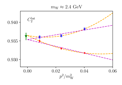
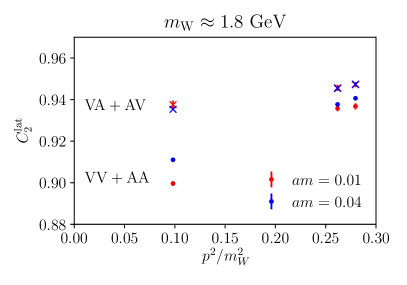
Figure 1: Left: Bare lattice Wilson coefficient $C_{2}$ measured on the 32I ensemble with twisted boundary conditions. Blue crosses correspond to the exceptional kinematics and red dots to the non-exceptional case. We show combined linear and quadratic extrapolations in $p^{2}/{m_{\mathrm{W}}}^{2}$ with a common constant term. For the final result, represented by a green diamond, we use a cubic fit whose larger statistical error covers the systematic uncertainty of the extrapolations. The data points have been obtained from parity odd $\gamma$ projectors. Right: $p^{2}$ dependence of $C_{2}^{\mathrm{lat}}$ for two different quark masses and parities of $\gamma$ projectors, labeled by the corresponding Dirac structure. A significant pole behavior is observed in the parity even case, signaling the contamination from non-perturbative physics. $\mathcal{CPS}$ symmetry arguments Bernard:1985wf ; Donini:1999sf also favor the parity odd case, where mixing with wrong chiralities is suppressed. Replacing $\gamma$ with $\not{q}$ projectors leads to the same considerations.

For a fixed set of projectors (odd/even and $\gamma$/$\not{q}$) we have verified that independent fits to the data with exceptional and non-exceptional kinematics give compatible results in the limit $p^{2}/{m_{\mathrm{W}}}^{2}\to 0$ within less than one standard deviation. Therefore we have decided to adopt combined fits with a common constant term for our final extraction, as reported in the left panel of Figure 1. With the present calculation we have not been able to separate QCD and weak scales enough, as $\Lambda_{\mathrm{QCD}}/{m_{\mathrm{W}}}\approx 0.15$, forcing us to push the calculation at very small momenta of $O(\Lambda_{\mathrm{QCD}})$, where non-perturbative effects may produce sizable contributions. In these proceedings we present results for the volume and quark mass dependence, which provide a qualitative understanding of these systematic errors. We refer the reader to Ref. wcoeff for a detailed and complete study of $O(\Lambda_{\mathrm{QCD}})$ effects.

4.2 Finite volume effects

To examine possible finite volume errors, we have repeated the calculation of the Wilson coefficients on the 16I and 24I ensembles, differing only in the volumes with $L\approx 1.8\leavevmode\nobreak\ \mathrm{fm}$ and $2.6\leavevmode\nobreak\ \mathrm{fm}$. Our results are plotted in the two panels of Figure 2, where we show measurements with exceptional kinematics only, from quark propagators with momenta injected along the $xy$ spatial directions and time ($t$). These choices explore the fact that each lattice has a temporal extent longer than the spatial one. In fact, for the 16I ensemble a noticeable difference in the limit of small $p^{2}/{m_{\mathrm{W}}}^{2}$ is visible with $\not{q}$ projectors between the two orientations of momenta; moreover when momentum is injected along the time direction the data points nicely overlap on the corresponding measurements on the 24I lattice, for which all different estimates agree with each other in the limit of small momenta. We interpret this behavior as the absence of finite volume errors: their presence spoils the convergence in the $p^{2}\to 0$ limit for fixed projectors and kinematics.

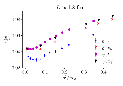
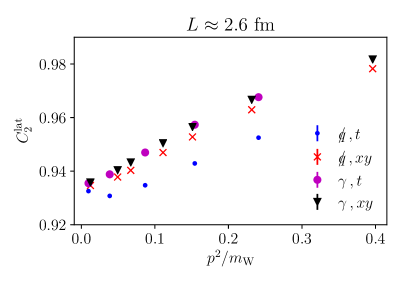
Figure 2: Wilson coefficient $C_{2}^{\mathrm{lat}}$ measured on the 16I and 24I ensembles with the same $W$ boson mass of approximately 1.8 $\mathrm{GeV}$. To exploit the different extents of the time and spatial directions, we have computed the quark propagators with momenta oriented along the $xy$ directions and $t$ alone. Results for (parity odd) $\gamma$ and $\not{q}$ projectors are reported as well. In the left panel the several measurements on the 16I do not agree with each other in the limit of small momenta, whereas the 24I shows a better agreement in the same limit.

4.3 Finite quark mass errors

The last infrared scale that we analyze in these proceedings is the quark mass. Ideally we would like to perform our calculation in a theory with mass-less quarks, but in practice all propagators have been computed at the strange quark mass of the corresponding ensemble. Hence, on the 24I we have studied the quark mass dependence by repeating the measurements with exceptional kinematics with $am=0.01$. The results are reported in the right panel of Figure 1. In this case the parity of the projectors plays a very important role. In the plot, where we show data only for allowed fourier modes, we observe a good agreement for parity odd projectors between the two masses studied and a rather strong behavior, approximately of the form $1/p^{2}$, for the opposite parity. In particular we note that increasing the quark mass suppresses the pole behavior, which we interpret as a non-perturbative effect due to the contamination of pseudo-scalar mesons to the amplitudes. For the central values of the Wilson coefficients we use the results from the parity odd sector, which in general is expected to show less contamination due to the suppression of the mixing with the wrong chiralities from $\mathcal{CPS}$ symmetry Bernard:1985wf ; Donini:1999sf . The difference between the two parities can be used as an estimate for the systematic uncertainties of the calculation, which turns out to be rather large ($\approx 2-3\%$) compared to the excellent statistical precision, which is below a percent. Residual chiral symmetry breaking effects are controlled by the separation of the two walls in the fifth dimension: for a few points we recomputed $C_{1}^{\mathrm{lat}}$ and $C_{2}^{\mathrm{lat}}$ with $L_{5}=32$ and we observed an excellent agreement with the original calculation at $L_{5}=16$ for all projectors.

4.4 Renormalization and continuum limit

For a comparison against known results in the continuum limit the appropriate renormalization factors have to be computed. First, we fix four values of the $W$ boson mass in physical units and we use the ratio of lattice spacings to tune them between the 24I and 32I ensembles. Second, to reproduce the initial conditions of the Wilson coefficients we measure the $Z$ factors at a renormalization scale equivalent to the four values of ${m_{\mathrm{W}}}$. Twisted boundary conditions allow us to reach these points in momentum space without problems and in the evaluation of the $Z$ factors we adopt the RI/SMOM conditions defined in Refs. Sturm:2009kb ; Lehner:2011fz . We also take the mass-less limit by repeating the calculation at two different quark masses and we perform a linear extrapolation in $m$.

The continuum limit is one of the important systematic effects to be addressed here. If the $W$ boson is too heavy compared to the cutoff, large discretization effects can appear in the Wilson coefficients, which essentially capture the modes around and above ${m_{\mathrm{W}}}$. The four values of the $W$ mass used here are $O(1)$ in lattice units. For $C_{2}^{\mathrm{RI}}$ a small lattice spacing error is found in the continuum extrapolations, well below 1%, while for $C_{1}^{\mathrm{RI}}$ it is larger, around 15%, partly due to the fact that the central value is much smaller ($C_{1}$ is 0 at tree-level).

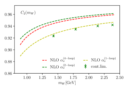
Figure 3: The data points are our results in the continuum limit for $C_{2}$ in the RI/SMOM scheme with $\gamma$ projectors. Only statistical errors are showed. The dashed lines correspond to the known 1-loop prediction in the ${\overline{\mathrm{MS}}}$ scheme with three definitions of the strong coupling constant obtained from 1, 2 and 4-loop $\beta$ functions (${\overline{\mathrm{MS}}}$).

Finally we present some preliminary results for the Wilson coefficients in the ${\mathrm{RI}}$ scheme, together with their prediction from perturbation theory in the ${\overline{\mathrm{MS}}}$ scheme. Note that the conversion factor $Z^{{\mathrm{RI}}\to{\overline{\mathrm{MS}}}}$ is currently missing from the calculation, an issue which we address in Ref. wcoeff for both $\gamma$ and $\not{q}$ intermediate schemes. For a qualitative comparison we present in Figure 3 the results from the $\gamma$ scheme where we expect the conversion matrix $Z^{{\mathrm{RI}}\to{\overline{\mathrm{MS}}}}$ to be very close to the identity Lehner:2011fz . An agreement with the perturbative predictions is found on a few percent level. We only display the statistical error bars without any estimate of systematic uncertainties or additional non-perturbative errors due to $O(\Lambda_{\mathrm{QCD}})$ effects. Recall that the difference between parity odd and even determinations, which is a good representative of such an error, is around 0.03 in absolute units.

The naive perturbative expansion of the Wilson coefficients in powers of $\alpha_{s}$ can be used, in principle, to determine the various coefficients of the first $n$-loop terms. In the situation where all systematic uncertainties have been addressed properly, fitting the Wilson coefficients reported in Figure 3 with a functional form like $C_{2}^{\mathrm{RI}}=1+k_{0}\alpha_{s}+k_{1}\alpha_{s}^{2}+\dots$ (and similarly for $C_{1}$ with tree-level value equal to 0) would allow us to predict them in the physical scenario, by running $\alpha_{s}$ to the physical $W$ pole, and to provide a concrete bound on the error of the initial conditions. Besides the difficulties mentioned above, a second caveat to take into account in such fits would be the flavor-dependence of the coefficients starting from two loops, which would require at least two simulations differing in the number of flavors in the sea. More details on how the current calculation can be extended to the physical scenario is given in Ref. wcoeff .

5 Conclusions

In these proceedings we have presented a method to compute the Wilson coefficients for the weak effective hamiltonian from lattice simulations. We have adopted a RI scheme and explored both the exceptional and non-exceptional kinematics in the extraction of the bare Wilson coefficients. By studying their dependence on the lattice size, on the quark mass and on the external states through different projectors, we have observed large non-perturbative effects that have to be included in the final systematic uncertainties.

We have demonstrated how our numerical strategy leads to results with small statistical errors. Already at this preliminary stage, without properly accounting for the differences in the renormalization schemes, we observe a relative good agreement with the known perturbative predictions. In a second publication we further advance this calculation by properly addressing all the systematic errors, with a more detailed and comprehensive study wcoeff .

References

- (1) G. Buchalla, A.J. Buras, M.E. Lautenbacher, Rev. Mod. Phys. 68, 1125 (1996), hep-ph/9512380
- (2) Z. Bai et al. (RBC, UKQCD), Phys. Rev. Lett. 115, 212001 (2015), 1505.07863
- (3) T. Blum et al., Phys. Rev. D86, 074513 (2012), 1206.5142
- (4) T. Blum et al., Phys. Rev. Lett. 108, 141601 (2012), 1111.1699
- (5) C. Kelly, EPJ Web Conf. LATTICE2017 (2017)
- (6) M. Gorbahn, U. Haisch, Nucl. Phys. B713, 291 (2005), hep-ph/0411071
- (7) C. Dawson, G. Martinelli, G.C. Rossi, C.T. Sachrajda, S.R. Sharpe, M. Talevi, M. Testa, Nucl. Phys. B514, 313 (1998), hep-lat/9707009
- (8) G. Martinelli, C. Pittori, C.T. Sachrajda, M. Testa, A. Vladikas, Nucl. Phys. B445, 81 (1995), hep-lat/9411010
- (9) Y. Aoki et al., Phys. Rev. D78, 054510 (2008), 0712.1061
- (10) C. Sturm, Y. Aoki, N.H. Christ, T. Izubuchi, C.T.C. Sachrajda, A. Soni, Phys. Rev. D80, 014501 (2009), 0901.2599
- (11) C. Lehner, C. Sturm, Phys. Rev. D84, 014001 (2011), 1104.4948
- (12) G.M. de Divitiis, R. Petronzio, N. Tantalo, Phys. Lett. B595, 408 (2004), hep-lat/0405002
- (13) R. Arthur, P.A. Boyle (RBC, UKQCD), Phys. Rev. D83, 114511 (2011), 1006.0422
- (14) Y. Aoki et al. (RBC, UKQCD), Phys. Rev. D83, 074508 (2011), 1011.0892
- (15) C. Allton et al. (RBC, UKQCD), Phys. Rev. D76, 014504 (2007), hep-lat/0701013
- (16) C.W. Bernard, T. Draper, A. Soni, H.D. Politzer, M.B. Wise, Phys. Rev. D32, 2343 (1985)
- (17) A. Donini, V. Gimenez, G. Martinelli, M. Talevi, A. Vladikas, Eur. Phys. J. C10, 121 (1999), hep-lat/9902030
- (18) M. Bruno, C. Lehner, A. Soni (2017), 1711.05768