The Second Data Release of the Beijing–Arizona Sky Survey

Abstract

This paper describes the second data release (DR2) of the Beijing–Arizona Sky Survey (BASS). BASS is an imaging survey covering a 5400 deg² footprint in the $g$ and $r$ bands using the 2.3 m Bok telescope. DR2 includes the observations through 2017 July obtained by BASS and by the Mayall $z$-band Legacy Survey (MzLS), which used the 4 m Mayall telescope to observe the same footprint. BASS and MzLS have completed 72% and 76% of their observations. The two surveys will be served for the spectroscopic targeting of the upcoming Dark Energy Spectroscopic Instrument. Both BASS and MzLS data are reduced by the same pipeline. We have updated the basic data reduction and photometric calibrations in DR2. In particular, source detections are performed on stacked images, and photometric measurements are co-added from single-epoch images based on these sources. The median 5$\sigma$ point-source depths after Galactic extinction corrections are 24.05, 23.61, and 23.10 mag for the $g$, $r$, and $z$ bands, respectively. The DR2 data products include stacked images, co-added catalogs, and single-epoch images and catalogs. The BASS website (http://batc.bao.ac.cn/BASS/) provides detailed information and links to download the data.

1 Introduction

Large-scale spectroscopic surveys over the past 20 years have revolutionized our view of the universe from the structure of the Milk Way and galaxy evolution to large-scale structure and dark energy (Colless et al., 2001; York et al., 2000; Scoville et al., 2007; Sánchez et al., 2012; Zhao et al., 2012; Newman et al., 2013; Liske et al., 2015). The Sloan Digital Sky Survey (SDSS; York et al., 2000) began with spectroscopy on the brightest targets in its imaging data. SDSS has since performed spectroscopy on progressively deeper targets, with SDSS-III/BOSS and SDSS-IV/eBOSS pushing to the faint limits of that imaging for the measurement of baryonic acoustic oscillations (Dawson et al., 2013, 2016). Deeper wide-field imaging data is required prior to the era of the Large Synoptic Survey Telescope (LSST; LSST Science Collaboration et al., 2009) to select targets for upcoming wide-field spectroscopic surveys, such as the Dark Energy Spectroscopic Instrument (DESI; DESI Collaboration et al., 2016) and Subaru Prime Focus Spectrograph (PFS; Takada et al., 2014).

DESI is a next-generation dark energy experiment that will accurately measure the expansion rate and structure growth of the universe. It will obtain spectroscopic redshifts of about 34 million galaxies and quasars, which is one magnitude more than those of the SDSS (DESI Collaboration et al., 2016). In addition to cosmology, the DESI project will play an important role in shaping our understanding of the Milky Way and galaxy evolution by observing stars and low-redshift galaxies during bright time.

The spectroscopic target selection for DESI will be based on three optical bands ($g$, $r$, and $z$) and two near-infrared bands ($W1$ and $W2$). The optical imaging surveys include three components: the Beijing–Arizona Sky Survey (BASS; Zou et al., 2017b), the Dark Energy Camera Legacy Survey (DECaLS; Blum et al., 2016), and the Mayall $z$-band Legacy Survey (MzLS; Silva et al., 2016). DECaLS covers a 9000 deg² equatorial footprint using the Dark Energy Camera (DECam) on the 4 m Blanco telescope at CTIO. BASS and MzLS, using the Bok and Mayall Telescopes, respectively, on Kitt Peak, are covering an adjacent 5000 deg² footprint in the north Galactic cap. All three optical surveys share a similar observing strategy. Dynamic exposure time calculators (ETCs) ensure their imaging depths will satisfy the requirement of the DESI spectroscopic target selection. The near-infrared images at wavelengths of 3.6 $\mu$m ($W1$) and 4.5 $\mu$m ($W2$) make use of the full-sky data from the $Wide$-$field$ $Infrared$ $Survey$ $Explorer$ mission (WISE; Wright et al., 2010) and the $NEOWISE$-$Reactivation$ data (Mainzer et al., 2014), coadded to their full depth (Meisner, Lang & Schlegel, 2017, 2018).

BASS is a $g-$ and $r$-band imaging survey that uses the wide-field 90Prime camera mounted on the 2.3 m Bok telescope (Williams et al., 2004). The observation started in 2015. It mainly covered gray and dark nights from January to July of each year. BASS had its early data and first data releases (DR1) in 2015 December and 2017 January (Zou et al., 2017a). DR1 only includes BASS data taken before 2016 July. By 2017 July, BASS has completed about 72% of the whole survey area. The MzLS covers the same area as BASS and have finished more than 76% of its observations by 2017 July. In this paper, we present the second BASS data release (DR2), which includes both BASS and MzLS data taken as of 2017 July.

This paper describes the details of BASS DR2. The paper is organized as follows. Section 2 presents basic information on the BASS and MzLS surveys and their observation status. Section 3 updates BASS data reduction. The source detection and photometry are described in Section 4. Section 5 presents the data quality and provides comparisons with other photometric surveys. Section 6 describes data access and provides guidelines for users. Section 7 is the summary.

2 BASS and MzLS Surveys

2.1 Telescope and instruments

Table 1 gives a summary of both the BASS and MzLS surveys. BASS uses the Bok telescope to image the northern part of the North Galactic cap with the optical $g$ and $r$ bands. The telescope is located on Kitt Peak near Tucson, Arizona. It is a 2.3 m telescope operated by Steward Observatory of University of Arizona. A wide-field camera, 90Prime, is mounted at the prime focus. It is composed of four 4k $\times$ 4k blue-sensitive CCDs, providing a feild of view (FoV) of 1°.08$\times$1°.03. The CCD pixel scale is about 0″.454. There are gaps between the CCDs and the filling factor is about 94%.

Table 1: A Summary of the BASS and MzLS Surveys

Telescope and Site	BASS	MzLS
Telescope	2.3 m Bok	4 m Mayall
Site	Kitt Peak	Kitt Peak
Elevation	2071 m	2071 m
Camera	BASS	MzLS
Name	90Prime	Mosaic-3
CCD number	4	4
CCD size	4096$\times$4032	4096$\times$4096
Gaps	168″ (R.A.), 54″ (Decl.)	52″ (R.A.), 62″ (Decl.)
Pixel scale	0″.45	0″.26
FoV	1°.08$\times$1°.03	36′$\times$36′
Gain	1.5 e/ADU	1.8 e/ADU
Readout noise	8.4 e	9 e
Readout time	35 s	30 s
Dark current	0.8 e/hr	0.9 e/hr
Filter	BASS	MzLS
Name	SDSS $g$, DECam $r$	DECam $z$
Wavelength	4789 Å, 6404 Å	9210 Å
Survey parameters	BASS	MzLS
Area	5400 deg2 ($\delta>30$°)	5100 deg2 ($\delta>32$°)
Expected Depth (5$\sigma$)	$g=24.0$, $r=23.4$	$z=23.0$
Observation period	2015–2018	2016–2017

MzLS uses the 4 m Mayall Telescope at Kitt Peak to image nearly the same area as BASS with the $z$ band. The telescope is located at the highest peak of the mountain, close to the Bok telescope. Its mirror diameter is about 4 m and its clear aperture diameter is about 3.8 m. The survey uses the Mosaic-3 imager deployed at the prime focus. It is a new wide-field imaging camera installed in mid-2015, replacing the old Mosaic-2 instrument. There are four 4k$\times$4k 500 $\mu$m thick deep-depletion CCDs, which significantly improved the $z$-band observing efficiency. The CCD pixel size is about 0″.26. The camera FoV is about 36′$\times$36′. Each CCD is read out through four amplifiers simultaneously. The readout time in the normal mode is about 30 s. The average gain and readout noise are 1.8 e/ADU and 9 e, respectively. The CCD quantum efficiency is optimized for red wavelengths, which can reach 85% at 900 nm. The dark current is 0.95 e/hr. More information about Mosaic-3 can be found in the camera manual.

In order to achieve homogeneous spectroscopic target selections for DESI, photometric systems of the imaging surveys should be as similar as possible. The DECaLS uses the DECam system, which is also used for the Dark Energy Survey (The Dark Energy Survey Collaboration, 2005). The BASS $g$ band is the existing SDSS $g$ filter. It is very close to the DECam $g$ band. The BASS $r$ filter is newly purchased by the Lawrence Berkeley National Laboratory, which is almost the same as the DECam $r$ band. The MzLS uses a newly purchased DECam $z$-band filter. Figure 1 shows the filter responses of these three filters. The response is the total throughput, including CCD quantum efficiency, filter transmission, and atmospheric extinction at the zenith, aluminum reflectivity of the prime mirror, and throughput of the optical corrector at the prime focus. The effective wavelengths for the BASS $g$ and $r$ and MzLS $z$ bands are 4789, 6404, and 9210 Å, respectively (see Table 2 for detailed filter parameters). For comparison, DECam filter responses are also plotted in Figure 1 and related parameters are presented in Table 2. The Galactic extinction coefficients are $k_{g}=$3.214, $k_{r}=$2.165, and $k_{z}=$1.211, which are adopted from the DECaLS webpage.

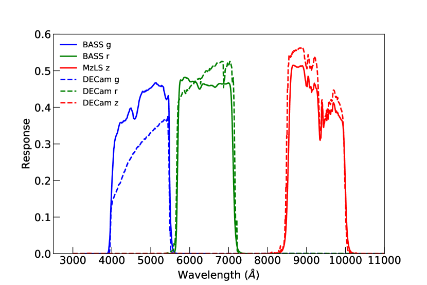
Figure 1: Filter response curves for BASS, MzLS, and DECaLS. All curves are the total responses.

Table 2: Parameters for BASS, MzLS and DECaLS filters.

	BASS $g$	BASS $r$	MzLS $z$	DECam $g$	DECam $r$	DECam $z$
Effective wavelength (Å)	4789	6404	9210	4842	6439	9172
Bandwidth (Å)	849	837	862	966	895	941
FWHM (Å)	1435	1420	1430	1290	1470	1470

2.2 Survey status

All DESI imaging surveys have similar observing strategies. Each survey tiles the sky in three passes or exposures. These three passes are dithered to fill CCD gaps. This is also benificial for detecting variable objects and allows zero-point determination with ubercalibration (Zou et al., 2017b). Pass 1 is observed in both photometric and good seeing conditions. Pass 2 is observed in either photometric or good seeing conditions. Pass 3 is observed in any other usable conditions. The seeing thresholds for BASS and MzLS are 1″.7 and 1″.3, respectively. Normally, $g$-band observation occur on dark nights, $r$-band observations occur on dark or gray nights, and $z$ band observations occur on gray and bright nights. The ETC can adjust the exposure time for each pass in real time according to sky brightness, seeing, atmospheric transparency, and Galactic extinction. In this way, both surveys can maintain uniform imaging depths for different passes.

BASS began its observation in 2015 January. The survey was awarded 55, 89, and 92 nights in the spring of 2015, 2016, and 2017, respectively. Since 2015, a number of updates have been implemented, such as instrument control software, telescope flexure maps, and observing tools, which greatly improved the pointing accuracy of the telescope, camera focusing, and observing efficiency. It was discovered that data taken in 2015 suffered from defective electronics in the read-out system, so these data were much noisier. Those electronics were replaced in 2015 September. The MzLS began regular observations in 2016 February. The imaging data suffered from variable crosstalk and pattern noise, which must specially treated. The MzLS has completed its scheduled with about 250 total observations. Figure 2 presents the observation progress as of 2017 July. Some test regions ($<100$ deg²) located at Cosmic Evolution Survey (COSMOS) and SDSS Stripe 82 fields are not shown in this figure. The BASS has completed about 72% of its scheduled observations, while the MzLS has completed about 76%. With typical observational conditions, BASS is expected to finish all observations in 2018, with an additional 100 nights. The MzLS completed the remaining observations before the Mayall telescope was shut down in 2018 February.

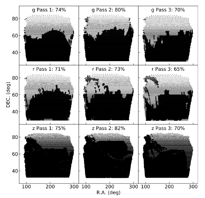
Figure 2: Observational progress for BASS and MzLS surveys as of 2017 July for different filters and passes. The percentage of area that has been observed is shown for each filter and pass.

3 Updates on Data Reduction

3.1 Image processing

The BASS and MzLS raw data are processed using the same pipeline. The basic corrections of overscan, bias, flat, and crosstalk effect are almost the same as those in BASS DR1. We make minor modifications when dealing with BASS data taken in 2015. The read-out mode was different in 2015. Bias frames were taken sequentially without flushing. Consequently, only the first bias frame can be used for bias subtraction. In addition, gain, readout noise, and crosstalk coefficients for each amplifier are calculated after the camera was remounted every summer. The identification of cosmic rays is also different in DR2. A Laplacian algorithm originating from van Dokkum (2001) was used to detect cosmic rays.

The crosstalk effect in MzLS data is much more serious than that in BASS data. The maximum intra-CCD crosstalk coefficient in MzLS reaches up to 5.2%, while for BASS it is only about 0.3%. There is also serious pattern noise in MzLS caused by the electromagnetic interference during CCD reading out, which is demonstrated in the left panel of Figure 3. We apply a low-pass filter to reconstruct the noise pattern. First, a 5-order low-pass Butterworth digital filter is designed by using the “butter” program in a Python package of SciPy . Then, the low-pass filter is applied to the source-removed $z$-band image and a smoothed pattern is constructed as shown in the middle panel of Figure 3. Finally, the pattern is subtracted from the original image as shown in the right panel of this figure.

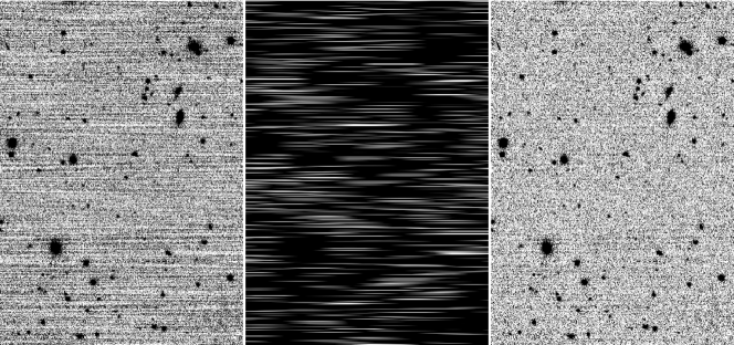
Figure 3: Removal of pattern noise in MzLS data. Left: raw image; middle: noise pattern constructed by a low-pass filter; right: image after pattern removal.

3.2 Astrometry

The Software for Calibrating AstroMetry and Photometry (SCAMP; Bertin, 2006) is used for calculating astrometric solutions. In DR1, the SDSS and Two Micron All Sky Survey (2MASS; Skrutskie et al., 2006) point-source catalogs were used as the reference catalogs. However, the Gaia (Gaia Collaboration et al., 2016) catalog is adopted in DR2. The first data release of Gaia (hereafter Gaia DR1; Gaia Collaboration et al., 2016) was published in 2016 September. It provides accurate astrometric measurements for objects in the $G$ band down to 20.5 mag over the entire sky. There are some images (about 1.5%) with faulty astrometry due to sparse sources in $Gaia$ catalogs, the 2MASS catalog is used to derive astrometric solutions for these.

Figure 4 gives a comparison of the astrometric accuracy when using different reference catalogs. The astrometric accuracy is much improved when using the $Gaia$ DR1 catalog as the reference. The median errors in R. A. and decl. are both about 28 mas. By contrast, if the SDSS catalog is used, the median errors in R. A. and decl. are about 93 mas.

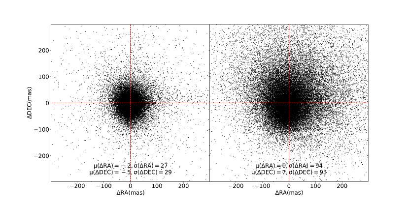
Figure 4: Astrometric accuracy using Gaia DR1 (left) and SDSS DR9 (right) as the reference catalogs. The data points are the same bright objects. The median offsets and RMS errors in R. A. and decl. are also shown in each panel. The horizontal and vertical dashed lines show zero offsets.

3.3 Zero-point calculation

As in DR1, the DR2 still uses Pan-STARRS1 data (hereafter PS1; Chambers et al., 2016) to derive photometric solutions. A large aperture diameter of 26 pixels is used for counting source fluxes. The aperture is equivalent to about 11″.9 for BASS and 6″.8 for MzLS (i.e. about 7 times the seeing FWHM). Point sources with S/N larger than 10 are selected and then matched to the PS1 catalogs with a cross-matching radius of 2″. The PS1 magnitudes are transformed to the BASS and MzLS photometric systems using the following equations:

$$(g-i) =g_{\rm PS1}-i_{\rm PS1},$$ (1)

$$g_{\rm BASS} =g_{\rm PS1}-0.08826+0.10575(g-i)-0.02543(g-i)^{2}+0.00226(g-i)^{3},$$ (2)

$$r_{\rm BASS} =r_{\rm PS1}+0.07371-0.07650(g-i)+0.02809(g-i)^{2}-0.00967(g-i)^{3},$$ (3)

$$z_{\rm MzLS} =z_{\rm PS1}+0.10164-0.08774(g-i)+0.03041(g-i)^{2}-0.00947(g-i)^{3}.$$ (4)

These color terms are valid for stars with $0.4<g-i<2.7$. The constant terms are kept to ensure no systematic offsets between BASS/MzLS and PS1. The zero-point of a CCD image is calculated as the error-weighted difference between instrumental aperture magnitudes and transformed PS1 PSF magnitudes with outliers removed.

In addition to the zero-point obtained with the external catalogs discussed above, we can also calculate an internal zero-point by using objects located in overlaps of different exposures. We have three passes for each field. Each pass has sufficiently large position offsets. For a specified image, an internal zero-point offset is calculated by comparing magnitudes of common objects in adjacent images. This offset is derived iteratively until its change is less than 0.001. We require that there are at least 50 stars to calculate the offset and the maximum number of iterations is 20. Normally, the computations for most images are converged after 10 steps. Figure 5 shows the distributions of the zero-point offsets for different filters. The dispersions are 0.005, 0.008 and 0.01 for $g$, $r$, and $z$ bands, respectively. Figure 6 gives an example of the performance of zero-point correction in one specially selected $g$-band image. This image is out of the PS1 coverage, so we use the Fourth US Naval Observatory CCD Astrograph Catalog to calculate a crude external zero-point. The histograms in this figure show the distributions of magnitude differences of common objects in multiple exposures before and after zero-point corrections are applied. We can see that after applying the corrections, both offset and scatter decrease. In practice, the internal zero point is used in DR2 only if the number of common stars are larger than 100 and its RMS error is less than 0.1. Otherwise the external zero-point is used.

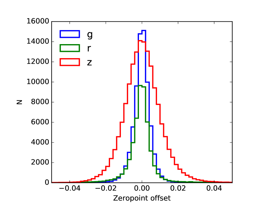
Figure 5: Distributions of internal zero point corrections for $g$ (blue), $r$ (green), and $z$ (red) bands.

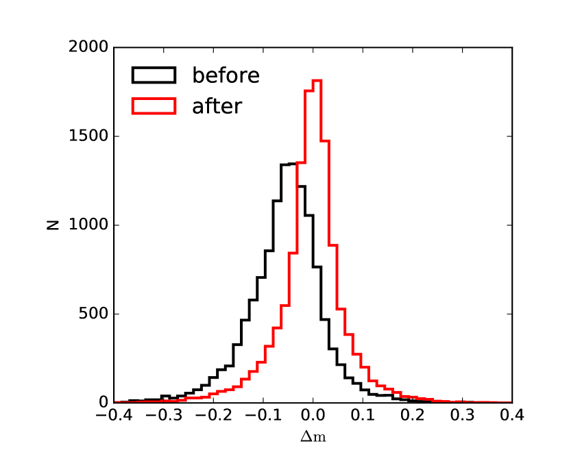
Figure 6: Distributions of magnitude differences of common objects in a $g$-band image and its adjacent images before (black) and after (red) internal zero point corrections are applied.

4 Photometry

There are significant changes in source detection and photometry between DR1 and DR2. In DR1, the source detection and corresponding photometry are performed on single-epoch images. However, we detect sources in stacked images in order to improve the detection efficiency in DR2. The DR2 photometry occurs in single-epoch images based on the positions of those sources.

4.1 Image stacking and source detection

As described in Zou et al. (2017a), the full sky is equally divided into 96,775 blocks. These blocks are evenly spaced in decl.. Each block has an area of 0°.681$\times$0.681 deg², equal to an image size of 5400 $\times$ 5400 with a pixel scale of 0″.454. There are overlaps of 0°.02 in both R.A. and decl. between adjacent blocks. The stacked image is generated with a simple tangent-plane projection around the block center.

We create four stacked images: three images for the $g$, $r$, and $z$ bands and one composite from these three stacks. The composite image is combined from $g$, $r$, and $z$-band stacked images with flux scales of 0.65, 1.0, and 1.5, respectively, which makes the $g-r$ and $r-z$ colors of F/G type stars close to zero. These flux scales are also used for generating color pictures. For a specified band and block, we collect single-epoch images that are connected to the block. These images are resampled and reprojected by Swarp and then combined by median to form a stacked image and corresponding weight image (Bertin et al., 2002). The sky background map for each single-exposure image is estimated by using a mesh with a grid size of 410 pixels and masking large objects from the Third Reference Catalog of bright galaxies (RC3) and New General Catalog (NGC). The flux of each single-epoch image is scaled to make the stack image have a photometric zero-point of 30 (i.e. magnitude is calculated as $m=-2.5\mathrm{log}_{10}F+30$). The single-epoch images used for stacking should satisfy the following conditions: (a) exposure time $>$ 30 s; (b) seeing $<$ 3″.5 for BASS and $<$ 2″.5 for MzLS; (c) zero-point RMS error $<$ 0.2; (d) number of stars used for calculating the zero-point $>$ 50; (e) astrometric RMS error in both R.A. and decl. $<$ 0″.5; (f) 5$\sigma$ depths are at most 1.5 mag shallower than the required one; (g) sky ADU $<$ 15,000 for BASS and $<$ 25,000 for MzLS; (h) transparency $>$ 0.5. Here the transparency is related to the level of atmospheric extinction. It is defined as $10^{0.4(\mathrm{zp_{0}}-\mathrm{zp})}$, where zp is the zero-point of an image corrected with airmass and $\mathrm{{zp}_{0}}$ is the typical zenith zero point on clear nights. Figure 7 gives examples of a $g$-band stacked image, its weight map, and corresponding color image composed of three-band stacked images.

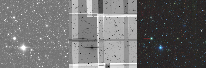
Figure 7: Left: a $g$-band stacked image of an arbitrary block. Middle: corresponding weight image. Right: color image combined from $g$, $r$, and $z$-band stacked images.

Source detections are performed first on the composite image and then separately on $g$-, $r$-, and $z$-band stacked images by SExtractor (Bertin & Arnouts, 1996). Objects are kept only if they are detected at least twice in those four images. In this way, a majority of fake sources with brightnesses close to the detecting threshold in each stacked image can be filtered out. Table 3 lists some key configuration parameters that significantly impact our detection and deblending. We chose a relative small threshold, minimum number of connected pixels, and convolution kernel so as to detect as many objects as possible for a single band. In addition, the minimum contrast parameter of “DEBLEND_MINCONST” is set to 0.001, which is determined as a compromise. A higher value will lead to more fragments of a large object and more fake sources within this object, while a lower value will give fewer fragments.

Figure 8 shows Kron elliptical apertures (see Section 4.2.3) of final detected sources on composite images. From the left and middle panels of this figure, we can see that the deblending algorithm is suitable for small and medium-sized galaxies (typical size of about 1 arcmin). For larger extended galaxies, the deblending method may not be appropriate due to bright foreground stars and substructures hesitated in these galaxies. We also notice that there are still some fake sources surrounding large bright stars or galaxies that are detected due to large noise fluctuation. As checked with external deep catalogs from COSMOS and DEEP2, about 8% of objects might be spurious. Most of these objects are located around bright stars and large galaxies. A few of them are probably CCD artifacts such as cosmic rays (especially in the $z$ band), which are not well identified by the imaging pipeline or not effectively removed due to a lack of enough exposure numbers.

Table 3: Key configuration parameters for source detection in SExtractor

Parameter	Value	Description
DETECT_MINAREA	3	Minimum number of pixels above threshold
THRESH_TYPE	RELATIVE	Threshold type
DETECT_THRESH	1.0	Detection threshold above the local background
FILTER_NAME	gauss_1.5_3x3.conv	Name of the file containing the filter for detection
CLEAN	N	Whether to clean spurious detections
DEBLEND_NTHRESH	64	Number of deblending sub-thresholds
DEBLEND_MINCONT	0.001	Minimum contrast parameter for deblending

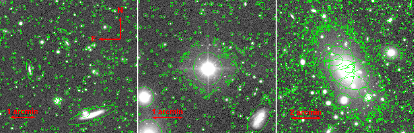
Figure 8: Detected sources overlain with Kron elliptical apertures . Left: normal galaxies and stars. Middle: detections around a bright star. Right: detections around a large galaxy. These images are displayed in a asinh scale to highlight the outer parts of sources more clearly.

4.2 Methods of photometry

We have developed a new Python-based package for photometry (H. Zou et al. in preparation). It can be used for more general purposes, but at present it is just applied to BASS DR2. The current code can make accurate measurements of circular aperture, elliptical aperture, and PSF magnitudes at specific positions. However, model measurements with galaxy profiles, such as deVauculeurs, exponential profiles, and composite profiles, are still in development. We describe a few key features below.

4.2.1 Segmentation and shape measurements

Different kinds of magnitude measurements are performed on a single-epoch image for objects detected on stacked images. These objects are first projected onto the image. A watershed segmentation algorithm is then adopted to separate signal pixels belonging to each object. The signal pixels are identified with a detecting threshold at 1$\sigma$ above the sky background after the image is smoothed with a Gaussian kernel of $\sigma$ = 1.5 pixels. The global sky background and its RMS map are calculated in mesh grids. Based on the segmentation of each object, we calculate the centroid, shape parameters, and refined center using a Gaussian-kernel window. The shape parameters describe the shape of an object as an ellipse, including semi-major ($A$) and semi-minor ($B$) axis lengths and position angle (PA). They are also called as $1\sigma$ elliptical parameters.

4.2.2 Circular aperture photometry

We adopt 12 apertures for circular aperture photometry with radii ranging from 3 to 40 pixels. These aperture sizes are the same as those used in the South Galactic Cap $u$-band Sky Survey, which utilized the Bok telescope and the 90Prime camera to perform a $u$-band imaging survey (Zou et al., 2015, 2016; Zhou et al., 2016). Table 4 shows the aperture radii in both pixels and arcseconds.

Table 4: Aperture Radii Used for Circular Photometry.

Aperture No.	1	2	3	4	5	6	7	8	9	10	11	12
Radius in pixel	3	4	5	6	8	10	13	16	20	25	30	40
Radius in arcsec (BASS)	1.36	1.82	2.27	2.72	3.63	4.54	5.90	7.26	9.08	11.35	13.62	18.16
Radius in arcsec (MzLS)	0.78	1.04	1.31	1.57	2.09	2.61	3.39	4.18	5.22	6.53	7.83	10.44

4.2.3 Isophotal and Kron elliptical aperture photometry

Isophotal magnitudes are derived by simply integrating pixel fluxes within segments. For better magnitude measurements of galaxies, we estimate an appropriate elliptical aperture for each object. The elliptical aperture should enclose most flux. We use the “Kron aperture”, which was introduced in Kron (1980). The Kron aperture size is described by the Kron radius. This radius is determined in a similar way as in SExtractor. First, a characteristic radius $r_{1}$ is calculated as the first-order moment within an large ellipse, whose size is 6 times the $1\sigma$ ellipse: $r_{1}=\frac{\sum{rF(r)}}{\sum{F(r)}}$, where $r$ is the elliptical distance of a pixel to the center and $F(r)$ is the corresponding flux in this pixel. We set the Kron radius $r_{k}$ to be 2.5$r_{1}$. The Kron aperture magnitudes are measured by integrating the fluxes of pixels within the Kron ellipse. The major and minor axis lengths of the Kron ellipse are computed as $r_{k}\sqrt{e}$ and $\frac{r_{k}}{\sqrt{e}}$, respectively, where $e$ is the elongation. To avoid extremely small and large apertures, we set lower and upper limits of the Kron radius to be 3$r_{0}$ and 10$r_{0}$, where $r_{0}=\sqrt{AB}$. It is shown that more than 94% of the light for galaxies is located in the Kron ellipse, almost independent of their magnitudes. For both circular and Kron aperture photometry, special handling is done for objects contaminated by nearby sources in order to improve the photometric accuracy. In the aperture, the pixels occupied by nearby objects are filled by mirroring the opposite pixels relative to the object center. In addition, each pixel is divided into 5$\times$5 sub-pixels to more accurately count the fluxes of pixels at the boundary of the aperture.

4.2.4 PSF photometry

PSF magnitudes are measured with the PSF model derived by PSFEx (Bertin, 2011). PSFEx models the PSF as a linear combination of basis vectors. The pixel basis and automatic sampling step are selected in this software. We use a third-degree polynomial to model the position-dependent variation of the PSF. The PSF size is 45$\times$45 for both BASS and MzLS, which is about 12 times the seeing FWHM. Table 5 lists some key input parameters in PSFEx. When fitting with the PSF model using our code, the pixels belonging to the segment of each object are used. If objects are not isolated, i.e. their segments are connected to each other, they are fitted simultaneously. We use k-means clustering to iteratively group objects. First, two groups are generated by the k-means clustering algorithm. Then the members in each group are divided into two subgroups using the same algorithm. All groups are divided in this way until the number of members in each group is not larger than three. Finally, all groups are ranked by their brightest members, and the PSF magnitudes in each group are measured simultaneously.

Table 5: Key input parameters for PSFEx

Parameter	Value	Description
BASIS_TYPE	PIXEL_AUTO	Type of basis vector
PSF_SAMPLING	0.0	Sampling step in pixel units
PSF_ACCURACY	0.01	Accuracy to expect from PSF ”pixel” values
PSF_SIZE	45, 45	Image size of the PSF model
PSF_RECENTER	Y	Whether to allow recentering of PSF-candidates
CENTER_KEYS	X_IMAGE, Y_IMAGE	Catalog parameters for source pre-centering
PSFVAR_DEGREES	3	Polynomial degree for position-dependent variation
SAMPLE_FWHMRANGE	2.0, 20.0	Allowed FWHM range
SAMPLE_VARIABILITY	0.5	Allowed FWHM variability
SAMPLE_MINSN	20	Minimum S/N
SAMPLE_MAXELLIP	0.3	Maximum ellipticity

4.3 Co-adding measurements

Based on the detections on stacked images, we perform circular aperture, isophotal, Kron elliptical aperture, and PSF flux measurements on single-epoch images. As described in our DR1 paper (Zou et al., 2017a), the coordinates of objects are corrected with astrometric residuals, which mainly origin from poor charge transfer efficiencies of detectors. The amount of corrections is about a few percent of an arcsecond. All magnitudes are aperture-corrected with growth curves produced by circular aperture photometry. In addition, magnitudes are corrected with photometric residuals, which are mainly caused by the focal distortion, improper flat-fielding, and scattered light. These astrometric and photometric residuals are obtained by comparing the coordinates and magnitudes with those in the Gaia DR1 and PS1 catalogs, respectively.

The parameters measured in single-epoch images are merged to generate co-added catalogs. For each object, we take weighted averages of the refined centers, shape parameters, and fluxes (equivalently magnitudes). Here, the weight is the inverse variance ($w=\frac{1}{\sigma^{2}}$). Thus, the errors of these averages come from errors of single-epoch measurements, which are computed as $\frac{1}{\sqrt{\Sigma w_{i}}}$, where $w_{i}$ is the weight. We also calculate the parameter standard error, which is rms of multiple parameter measurements divided by the square root of the number of measurements. The standard error including all possible error sources is a more realistic error estimation. Particularly, a large magnitude standard error for a variable star indicates light variation. The effective seeing and sky background, number of exposures, and average, minimum, and maximum of the Julian day when observations were taken, are recorded in the catalogs.

5 Data Analyses and Comparisons

5.1 Data quality of single-epoch images

The ETC ensures our imaging depths to meet the requirements, although the observing strategy entails different passes being observed under different weather conditions. Table 6 presents median observational and imaging parameters for different filters. The $z$-band seeing is the best. The depth is estimated as the median PSF magnitude at the error of about 0.21 mag (5$\sigma$). The single-epoch depths are 23.3, 23.1, and 22.6 mag for the $g$, $r$, and $z$ bands, respectively. We also have checked that the depths for different passes of the same filter are quite similar owing to the ETC.

Table 6: Median observational and imaging parameters for single-epoch images

	Area	Seeing	Sky	Airmass	Zero-point	Depth
	(a)	(b)	(c)	(d)	(e)	(f)
$g$	75%	1.60	22.09	1.05	25.92	23.33
$r$	70%	1.42	21.27	1.05	25.81	23.06
$z$	76%	1.04	18.96	1.05	26.46	22.59

5.2 Co-added Depths

The depth requirements for DESI are 23.91, 23.47, and 22.60 mag for the $g$, $r$, and $z$ bands, respectively, which are defined by 5$\sigma$ extended sources with a correction of Galactic extinction and converted to our photometric systems with color terms as shown in Equation (4). The Galactic reddening map comes from Schlegel et al. (1998). We estimate the $5\sigma$ depths by using co-added PSF magnitude errors. Figure 9 shows the depth distributions of all blocks with exposure numbers equal to 3. They are so-called “full depth,” with three complete passes. The $g$-band distribution has a fatter tail at the bright end. Because of this we include the data taken in 2015. These data were shallower due to the imperfect ETC and problematic due to bad A/D converters. The low bits of ADU integers were lost. This seriously affects the photometry of faint sources. This issue mostly affects the $g$-band images. Some of the affected areas have been re-observed in recent years and will be totally covered in future observations. Table 7 lists the median depths and fractions of objects for different exposure numbers. The median 5$\sigma$ depths for the $g$, $r$, and $z$ bands are 24.05, 23.61, and 23.10 mag, respectively. Most of the area covered by the $g$ band has more than 3 exposures due to duplicate observations from 2015.

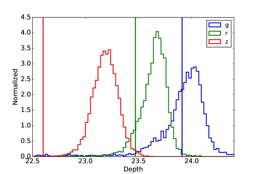
Figure 9: Normalized distributions of full depths estimated by $5\sigma$ PSF magnitude errors for the $g$, $r$, and $z$ bands. The vertical lines indicate the DESI required depths.

Figure 10 shows the number counts of objects in the $g$, $r$ and $z$ bands in the regions of DEEP2 fields. The Kron magnitude is adopted here, which is a good brightness measurement for both stars and galaxies. The DEEP2 photometric data were taken with the CFH12K camera on the 3.6 m Canada-France-Hawaii Telescope and cover about 5 deg² over the sky, with completeness limits of $B=25.25$, $R=24.75$, and $I=24.25$ mag (Coil et al., 2004). We overplot the $R$-band number count in Figure 10 after the $R$-band magnitude is converted to BASS $r$ using a color term based on $B-R$. In general, the BASS and MzLS completeness limits reach or exceed the nominal DESI depths and the $r$-band magnitude distribution matches well with the DEEP2 $R$-band distribution. About 2% of objects have BASS $r$-band exposure numbers less than 3, so corresponding magnitude limits are about 0.3–0.6 mag shallower. This causes a slightly lower number count at $r\sim 22$. In addition, different photometric systems and photometric methods between BASS and DEEP2 might also affect the discrepancy of the magnitude distribution. The co-added depths are 1.5–2.5 mag deeper than the SDSS imaging. For a visual comparison, we demonstrate the imaging data around a group of galaxies from both BASS/MzLS and SDSS in Figure 11. There are many more fainter objects that can be seen in BASS/MzLS images. The SDSS $z$-band is much shallower, leading to a much noisier background.

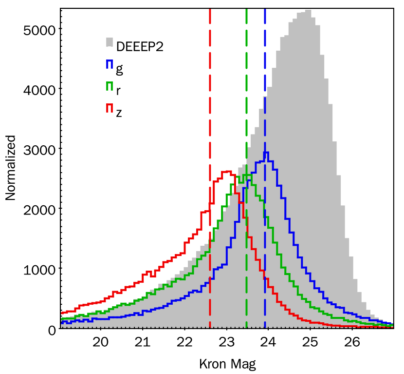
Figure 10: Kron magnitude distributions of sources located in DEEP2 fields. The nominal DESI depths are plotted as dashed vertical lines. The filled gray histogram shows the DEEP2 $R$-band magnitude distribution after it is converted to the BASS $r$ band using a system transformation.

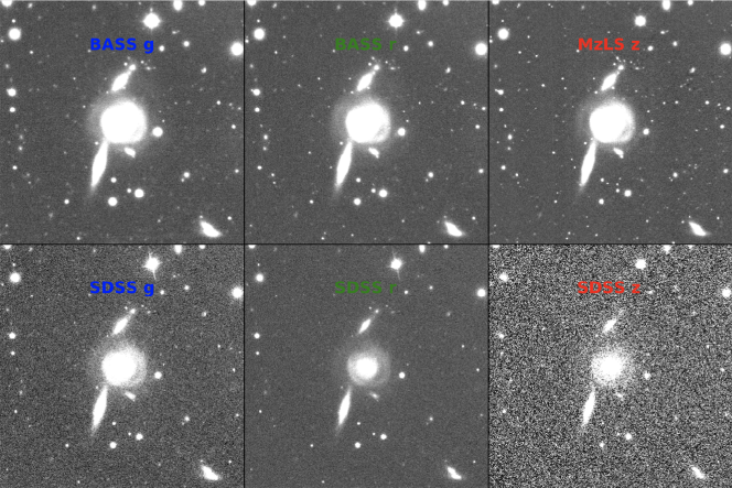
Figure 11: Imaging comparison between BASS/MzLS and SDSS. The scale for each band is the same.

Table 7: Imaging depths and fractions of objects with different exposure numbers

	Median Depth			Fraction
	$g$	$r$	$z$	$g$	$r$	$z$
1	23.31	22.99	22.63	5.7%	9.6%	13.7%
2	23.74	23.44	22.98	11.9%	18.6%	28.5%
3	23.91	23.64	23.18	18.1%	43.2%	38.6%
$\geq 4$	24.12	23.80	23.38	64.3%	28.6%	19.2%
median	24.05	23.61	23.10	$\cdots$	$\cdots$	$\cdots$

5.3 Photometric comparisons

The DECaLS has released its DR5 in 2017 June. Its typical depths with three exposures are 24.7, 23.6 and 22.8 mag for the $g$, $r$, and $z$ bands, respectively. The $g$-band and $r$-band depths are a little deeper than those of BASS DR2, while the $z$ band is somewhat shallower. There are some overlaps between DECaLS and BASS observations. These two surveys almost cover the whole SDSS footprint, but they are 1.5–2.5 mag deeper. We show some photometric comparisons of the three surveys with the data in the overlapping area. Figure 12 shows the magnitude difference as function of magnitude for point sources, which are randomly selected based on the morphological type in DECaLS DR5. The DECaLS and SDSS data are both transformed to the BASS/MzLS photometric systems using different color terms. The photometric scatters of point sources brighter than 20 mag between DECaLS and BASS are about half of those between SDSS and BASS. We also compare the color-color diagrams of three surveys with the same dataset ($r<23$ mag), as shown in the upper panels of Figure 13. The color distributions of $g-r$ at $r-z\sim 1.6$ and $r-z$ at $g-r\sim 0.7$ are also shown in the middle and bottom panels of Figure 13. The standard deviations of the color distributions are annotated in each panel. From these plots, we can see that BASS DR2 is as good as DECaLS DR5, and it is obviously better than the SDSS data.

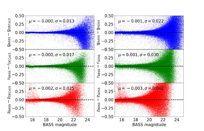
Figure 12: Magnitude difference as a function of BASS magnitude between BASS and DECaLS (left panels) and between BASS and SDSS (right panels). The $g$, $r$, and $z$ bands are plotted in blue, green, and red in the top, middle and bottom panels, respectively. The magnitude average offset and scatter of stars brighter than 20 mag are shown in each panel. The horizontal dashed lines show zero offsets.

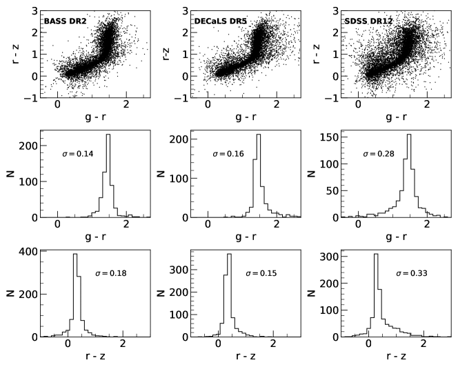
Figure 13: Top row: color-color diagrams in $g-r$ vs. $r-z$. Middle row: $g-r$ color distribution at $r-z\sim 1.6$. Bottom row: $r-z$ color distribution at $g-r\sim 0.7$. From left to right, the panels display BASS DR2, DECaLS DR5, and SDSS DR12, respectively.

6 Data Access and Guidelines for DR2

6.1 Data Access

Information about the surveys, such as the telescopes, instruments, and observations, can be retrieved on the public data release website. The data cover the observations between 2015 January and 2017 July. There are 297,367 calibrated single-epoch CCD images. Those images with zero-point calibrations have corresponding catalogs. There are 13,419 blocks in total that have stacked images. For each block, there are three stacked images for the $g$, $r$, and $z$ bands and one co-added catalog. The summary files for single-epoch images and blocks can be found on the webpage. Figure 14 shows the sky coverage of the DR2 catalogs. In addition to the regular survey area as shown in a green envelope, there are some test regions (e.g. COSMOS and Stripe 82) and scattered regions with observations shared with BASS by other observers.

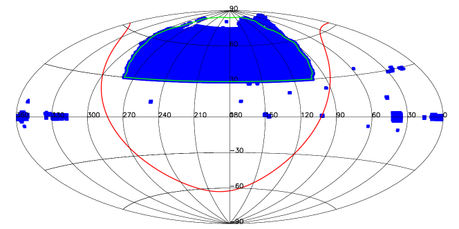
Figure 14: Sky coverage of the DR2 co-added catalogs in Aitoff projection. The region outlined in green indicates the regular survey area. The red curve shows the Galactic plane.

Access to DR2 data is provided by the Chinese Virtual Observatory. Select data can be acquired from the following links.

1. DR2 release webpage: http://batc.bao.ac.cn/BASS/doku.php?id=datarelease:dr2:

2. To search for single-epoch image and catalog files: http://explore.china-vo.org/data/bassdr2images/f

3. To search for stacked image and co-added catalog files: http://explore.china-vo.org/data/bassdr2stack/f

4. To search for sources in co-added catalogs: http://explore.china-vo.org/data/bassdr2coadd/f

5. To generate “wget” scripts for downloading files: http://batc.bao.ac.cn/BASS/doku.php?id=datarelease:dr2:dr2_wgetbulk:

6. Sky viewer for visualizing the data: http://batc.bao.ac.cn/BASS/doku.php?id=datarelease:dr2:dr2skyviewer:

The sky viewer is based on Aladin HiPS .

6.2 A few guidelines for using the data

6.2.1 Images

The calibrated single-epoch images have astrometric and photometric solutions stored in the FITS header. The flux units in the images are e/s. For each image, we have corresponding weight and flag images. The flag image tags the problematic pixels, the same as in DR1. We summerize useful parameters for single-epoch images in a FITS table and the user can find the column description on the wiki page. The single-epoch images with the column “imq” $=$ 1 are used for generating stacked images and co-added catalogs. There are several columns, as shown in Table 8, that denote astrometry qualities and zero-point. The “astr_ref” have two options: GAIA-DR1 and 2MASS. Usually, the astrometric accuracy obtained from using 2MASS as the reference catalog is worse than that using the Gaia catalog. The internal and external zero-points are combined as “zp”, which is used in our photometry. The magnitude can be calculated as $m=-2.5\mathrm{log}_{10}F+\mathrm{zp}$, where $F$ is the integrated flux of an object. Note that the single-epoch images have both astrometric and photometric residuals even though we can correct them in the catalogs. If the user wants higher accuracies for the astrometry and photometry from images, one should apply the residual maps to the coordinates and magnitudes. The astrometric correction can be as much as 0″.04 for both BASS and MzLS. The photometric correction can be as much as 0.02 and 0.05 mag for BASS and MzLS, respectively.

Table 8: Key Columns Describing Astrometry and Zero-point in the Summary File of CCD Images

Column	Unit	Description
ra_off	arcsec	R.A. offset relative to the reference catalog
dec_off	arcsec	Decl. offset relative to the reference catalog
ra_rms	arcsec	R.A. rms relative to the reference catalog
dec_rms	arcsec	Decl. rms relative to the reference catalog
astr_num	$\cdots$	Number of stars used for statistics of astrometric parameters
astr_ref	$\cdots$	Reference catalog for astrometry
zp	mag	Combined zero-point
zp_rms	mag	Combined zero-point rms
zp_num	$\cdots$	Number stars for combined zero-point

The stacked images cannot be used for accurate photometric measurements because they are combined from many single-epoch images with different qualities. Each stacked image has a weight image. We adopt standard WCS parameters with a simple “TAN” projection. The zero-points are fixed to 30.

6.2.2 Catalogs

The co-added catalogs provide the deepest and most accurate magnitude measurements for objects with multiple exposures. A co-added catalog covers an area of about 0.68$\times$0.68 deg² with an 0°.02 overlap with other neighboring blocks. For each source in the catalog, we provide the minimums, maximums, and averages of modified Julian date, seeing in FWHM, sky brightness, and zero-point from single-epoch observations, and provide the total exposure time and number of exposures in each band. The catalogs include Galactic reddening from the map of Schlegel et al. (1998), some measurements from stacked images derived by SExtractor, such as shape parameters and star/galaxy classification (marked with a postfix “_Stack”), and “Mag_Auto” magnitudes for three bands. These measurements are only recorded and much less accurate. The other measurements in the catalogs are obtained by co-adding parameters from single-epoch images by our own photometric code. For each band, there are coordinates, shape parameters (e.g. half major/minor axis length, ellipticity, PA and Kron radius), all kinds of fluxes and magnitudes, and flags. For the magnitude error, we provide both normal parameter error and standard error. The standard error is related to the magnitude rms of multiple observations. It contains information of light variation, which can be useful for variable objects. Shape parameters are directly computed from the images. They are not intrinsic due to the seeing effect. The single-epoch catalogs contains the measurements for objects detected on stacked images. The object ID is unique in the co-added catalogs, while objects in single-epoch catalogs use the same ID. This means that the ID in single-epoch catalogs can be duplicated for objects with multiple observations. All fluxes in the catalogs are in nanomaggy, where magnitudes can be calculated as $-2.5\mathrm{log}_{10}F+22.5$. We recommend the PSF magnitude for point sources and Kron magnitudes for extended sources. For very large galaxies with apparent diameters larger than about 1′, they might be fragmented due to foreground stars and their substructures, which might mean the photometry might not be reliable.

For star/galaxy separation, the column “Type_Stack” gives a median of class parameters from stacked images derived by SExtractor. We can also identify point sources from the reduced $\chi^{2}$ of PSF fitting. The reduced $\chi^{2}$ can be computed as the ratio of “Chi2_PSF” and “DOF_PSF” columns in the catalogs. If it is close to 1, the object is likely to be a point-like source. In addition, the ellipticity, color, and magnitude difference between PSF and Kron magnitudes can be also useful for classification. The user can even combine all these parameters to separate objects. We expect a classification to be added in the next data release.

7 Summary

The BASS made its first data release be public in 2017 January. It only includes the BASS $g$-band and $r$-band observations taken before 2016 July. This paper describes the details of our second data release, which include new datasets and updates to the data reduction. We summarize these updates as follows:

1. The DR2 includes the data taken as of 2017 July. This release includes the MzLS data. The BASS and MzLS have respectively completed about 72% and 76% of their observations over the footprint of over 5000 deg².

2. BASS and MzLS data are reduced by the same pipeline, which includes some updates from DR1, such as bias correction of 2015 BASS data, identification of cosmic rays, crosstalk correction, and subtraction of pattern noise in MzLS images.

3. Gaia DR1 catalogs are utilized to derive astrometric solutions. The global astrometric error is about 0″.03. This is much better than DR1, where SDSS DR9 was used as the reference catalog.

4. External photometric zero-points are calculated using point-source catalogs of PS1, the same as in DR1. To improve the accuracy of flux calibrations, internal zero-points are computed by comparing the magnitude differences of common objects in different exposures.

5. Source detection is implemented in stacked images and photometry is made in single-epoch images. We provide circular aperture, Isophotal, Kron elliptical aperture, and PSF magnitudes. The median depths over the whole coverage are 24.05, 23.61, and 23.10 mag for the $g$, $r$, and $z$ bands, respectively.

6. The DR2 data products include calibrated single-epoch images, single-epoch catalogs, stacked images, and co-added catalogs. They can be accessed through links in the BASS data release webpage (http://batc.bao.ac.cn/BASS/doku.php?id=datarelease:dr2:).

The MzLS finished its observations in February of 2018 and the BASS will complete the observations in of 2019 January. The next data release (DR3) is expected to include all BASS and MzLS survey data. Furthermore, we will have some new features in DR3, such as astrometry by Gaia DR2, a new source detecting algorithm, a star-galaxy separation, a flag to mark objects close to bright stars and large galaxies, new PSF modeling, and Galactic extinction from Planck dust map.

References

- Bertin & Arnouts (1996) Bertin, E., & Arnouts, S. 1996, A&AS, 117, 393
- Bertin (2006) Bertin, E. 2006, Astronomical Data Analysis Software and Systems XV, 351, 112
- Bertin (2011) Bertin, E. 2011, Astronomical Data Analysis Software and Systems XX, 442, 435
- Bertin et al. (2002) Bertin, E., Mellier, Y., Radovich, M., et al. 2002, Astronomical Data Analysis Software and Systems XI, 281, 228
- Blum et al. (2016) Blum, R. D., Burleigh, K., Dey, A., et al. 2016, American Astronomical Society Meeting Abstracts, 228, 317.01
- Chambers et al. (2016) Chambers, K. C., Magnier, E. A., Metcalfe, N., et al. 2016, arXiv:1612.05560
- Coil et al. (2004) Coil, A. L., Newman, J. A., Kaiser, N., et al. 2004, ApJ, 617, 765
- Colless et al. (2001) Colless, M., Dalton, G., Maddox, S., et al. 2001, MNRAS, 328, 1039
- Dawson et al. (2013) Dawson, K. S., Schlegel, D. J., Ahn, C. P., et al. 2013, AJ, 145, 10
- Dawson et al. (2016) Dawson, K. S., Kneib, J.-P., Percival, W. J., et al. 2016, AJ, 151, 44
- DESI Collaboration et al. (2016) DESI Collaboration, Aghamousa, A., Aguilar, J., et al. 2016, arXiv:1611.00036
- Doi et al. (2010) Doi, M., Tanaka, M., Fukugita, M., et al. 2010, AJ, 139, 1628
- Gaia Collaboration et al. (2016) Gaia Collaboration, Brown, A. G. A., Vallenari, A., et al. 2016a, A&A, 595, A2
- Gaia Collaboration et al. (2016) Gaia Collaboration, Prusti, T., de Bruijne, J. H. J., et al. 2016b, A&A, 595, A1
- Kron (1980) Kron, R. G. 1980, ApJS, 43, 305
- Liske et al. (2015) Liske, J., Baldry, I. K., Driver, S. P., et al. 2015, MNRAS, 452, 208
- LSST Science Collaboration et al. (2009) LSST Science Collaboration, Abell, P. A., Allison, J., et al. 2009, arXiv:0912.0201
- Mainzer et al. (2014) Mainzer, A., Bauer, J., Cutri, R., et al. 2014, ApJ, 792, 30
- Meisner, Lang & Schlegel (2017) Meisner, A.M., Lang, D., & Schlegel, D.J. 2017, AJ, 153, 38
- Meisner, Lang & Schlegel (2018) Meisner, A.M., Lang, D., & Schlegel, D.J. 2018, RNAAS, 2, 1
- Newman et al. (2013) Newman, J. A., Cooper, M. C., Davis, M., et al. 2013, ApJS, 208, 5
- Sánchez et al. (2012) Sánchez, S. F., Kennicutt, R. C., Gil de Paz, A., et al. 2012, A&A, 538, A8
- Schlegel et al. (1998) Schlegel, D. J., Finkbeiner, D. P., & Davis, M. 1998, ApJ, 500, 525
- Scoville et al. (2007) Scoville, N., Aussel, H., Brusa, M., et al. 2007, ApJS, 172, 1
- Silva et al. (2016) Silva, D. R., Blum, R. D., Allen, L., et al. 2016, American Astronomical Society Meeting Abstracts, 228, 317.02
- Skrutskie et al. (2006) Skrutskie, M. F., Cutri, R. M., Stiening, R., et al. 2006, AJ, 131, 1163
- Takada et al. (2014) Takada, M., Ellis, R. S., Chiba, M., et al. 2014, PASJ, 66, R1
- The Dark Energy Survey Collaboration (2005) The Dark Energy Survey Collaboration 2005, arXiv:astro-ph/0510346
- van Dokkum (2001) van Dokkum, P. G. 2001, PASP, 113, 1420
- Williams et al. (2004) Williams, G., Olszewski, E., Lesser, M., & Burge, J. 2004, SPIE, 5492, 787
- Wright et al. (2010) Wright, E. L., Eisenhardt, P. R. M., Mainzer, A. K., et al. 2010, AJ, 140, 1868-1881
- York et al. (2000) York, D. G., Adelman, J., Anderson, J. E., Jr., et al. 2000, AJ, 120, 1579
- Zhao et al. (2012) Zhao, G., Zhao, Y.-H., Chu, Y.-Q., Jing, Y.-P., & Deng, L.-C. 2012, Research in Astronomy and Astrophysics, 12, 723
- Zhou et al. (2016) Zhou, X., Fan, X.-H., Fan, Z., et al. 2016, Research in Astronomy and Astrophysics, 16, 69
- Zou et al. (2015) Zou, H., Jiang, Z.-J., Zhou, X., et al. 2015, AJ, 150, 104
- Zou et al. (2016) Zou, H., Zhou, X., Jiang, Z., et al. 2016, AJ, 151, 37
- Zou et al. (2017a) Zou, H., Zhang, T., Zhou, Z., et al. 2017, AJ, 153, 276
- Zou et al. (2017b) Zou, H., Zhou, X., Fan, X., et al. 2017, PASP, 129, 064101