Violating the Energy-Momentum Proportionality of Photonic Crystals in the Low-Frequency Limit

Abstract

We theoretically show that the frequency and momentum of a photon are not necessarily proportional to one another at low frequencies in photonic crystals comprising materials with positive- and negative-valued material properties. We rigorously determine closed-form conditions for the light cone to emanate from points other than the origin of $k$ space, ultimately decoupling the first band from the origin and demonstrating light propagation at zero energy with nonzero crystal momentum. We also numerically show that first bands can originate from an arbitrary Bloch coordinate as well as from multiple coordinates simultaneously.

When a photon propagates through a dielectric medium at low frequencies, it satisfies the energy-momentum ($E$-$k$) relation $E=c\hbar|\mathbf{k}|$, where $c$ is the phase velocity in the medium Joannopoulos et al. (2008); Born and Wolf (1964). This relation ensures that at zero energy, the photon possesses zero momentum. Fundamental relations of this type are prevalent throughout nature and are not isolated to photons, for example, electrons propagate through a crystal lattice as $E=\hbar^{2}/(2m_{\mathrm{eff}})|\mathbf{k}|^{2}$ at low energies, where $m_{\mathrm{eff}}$ is the effective mass Kittel (2005). This proportionality is fundamental for the study of particles and fields in relativistic mechanics, particle physics, and quantum mechanics.

In this Letter, we break the conventional low-frequency $E$-$k$ proportionality for photons, obtaining relations of the form $E=C\,|\mathbf{k}-\Xi|$, where $\Xi$ denotes a high-symmetry point of the reciprocal lattice and $\mathbf{k}$ is the crystal momentum (see Figs. 1a-c). This is achieved in two-dimensional photonic crystals comprising materials with positive-definite and negative-definite Smith et al. (2004); Veselago (1968); Pendry (2000) optical properties. We present explicit conditions on the constituent properties and explicit forms for the proportionality constants $C$, for all high-symmetry coordinates of a square lattice. Furthermore, we numerically demonstrate the existence of other novel low-frequency behaviors, including photonic crystals with $E=C_{1}\,|\mathbf{k}|+C_{2}\,|\mathbf{k}-\mathbf{X}|$, where $C_{j}$ are proportionality constants and $X$ is a high-symmetry point (see Fig. 3e). Such unconventional behavior contrasts the standard outcomes for light in photonic crystals, where either $E$-$k$ proportionality is supported, or there exists a complete band gap Fan et al. (1996), at low frequencies.

In the nonstandard photonic settings we describe, massless photons are predicted to propagate as massive polaritons which travel superfluidically through the medium Lerario et al. (2017). Consequently, our findings have the potential to motivate the development of new photonic devices, and to deepen our understanding of light in structured media. The behaviors we describe complement existing observations in optical systems incorporating negative-definite materials, such as folded band surfaces with infinite group velocities Chen et al. (2011), cloaking and superresolution Guenneau et al. (2007); Helsing et al. (2011), and new types of band gaps Li et al. (2003). Analogies to our low-frequency $E$-$k$ relations may be found in the electronic properties of transition-metal perovskites, where the first band is centered about high symmetry points other than the origin Harrison (1989); Cora et al. (1997).

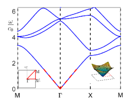
(a)

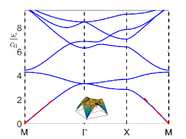
(b)

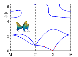
(c)

Figure 1: Band diagrams for square array of cylinders embedded in air with LABEL:sub@fig:conventionalGamma1 $\varepsilon_{\mathrm{c}}=1$ and $\mu_{\mathrm{c}}=2$, LABEL:sub@fig:Mptex1 $\varepsilon_{\mathrm{c}}=-1$ and $\mu_{\mathrm{c}}=2$, and LABEL:sub@fig:Xpics1 $\varepsilon_{\mathrm{c}}\approx-0.53$ and $\mu_{\mathrm{c}}\approx-10.22$. Dashed red lines denote low-frequency descriptions (3), (5), and (8b), respectively. All figures use lattice period $a=1$, radius $a^{\prime}=0.3a$, and dipolar approximation. Inset: first Brillouin zone with path parametrization $\Gamma$$X$$M$; first band surfaces over first Brillouin zone.

We begin by considering the modes of the time-harmonic form of the source-free Maxwell equations in a nondispersive and lossless system with Bloch vectors $\mathbf{k}=(k_{x},k_{y},0)$. This wave vector restriction reduces Maxwell’s equations to the Helmholtz equation

$$\nabla_{\perp}\cdot\left(\varepsilon_{\mathrm{r}}^{-1}\nabla_{\perp}H_{\mathrm{z}}\right)+\omega^{2}c_{0}^{-2}\mu_{\mathrm{r}}H_{\mathrm{z}}=0,$$ (1)

for fields polarized as $\mathbf{H}=(0,0,H_{\mathrm{z}})$. Here, $\nabla_{\perp}\equiv(\partial_{\mathrm{x}},\partial_{\mathrm{y}})$, $\varepsilon_{\mathrm{r}}$ is the relative permittivity, $\mu_{\mathrm{r}}$ the relative permeability, $\omega$ the angular frequency, and $c_{0}$ is the speed of light in vacuum. We consider an array of infinitely extending isotropic cylinders, periodically positioned in the $(x,y)$ plane at the coordinates of a square lattice, and which are embedded in an infinitely extending isotropic background material. In the background and cylinder domains, material constants are allowed to be negative-valued. At the cylinder edges we impose continuity conditions, and between unit cells we impose Bloch–Floquet conditions. This admits the system Movchan et al. (2002)

$$N_{l}\mathcal{B}_{l}+\sum_{m=-\infty}^{\infty}(-1)^{l+m}S_{m-l}^{\mathrm{Y}}\mathcal{B}_{m}=\boldsymbol{0},$$ (2)

where $S_{m}^{\mathrm{Y}}=S_{m}^{\mathrm{Y}}(\omega_{\mathrm{B}},\mathbf{k}_{\mathrm{B}};n_{\mathrm{b}})$ denotes lattice sums (see Supplemental Material sup ), $\omega_{\mathrm{B}}=\omega/c_{0}$, $\mathbf{k}_{\mathrm{B}}=(k_{x},k_{y})$, $\mathcal{B}_{m}$ are amplitudes of the cylindrical-harmonic basis functions, and $N_{m}$ are inverse cylindrical-Mie coefficients. Where applicable, subscripts $\mathrm{b}$ and $\mathrm{c}$ denote the background and cylinder properties, respectively. The dispersion equation for the crystal is given by the vanishing determinant of (2), which we truncate to dipolar order.

We now outline the procedure for determining when a low-frequency band surface emerges from the $\Gamma$ point. First, we evaluate expansions for $N_{m}$ in $\omega_{\mathrm{B}}$ (these are lengthy, see Supplemental Material sup ). Next, we determine closed-form expressions for the $S_{l}^{\mathrm{Y}}$ in (2) at low frequencies and about the $\Gamma$ point; these are obtained following Chen et al. (2018) (also extensive, see Supplemental Material sup ). Assuming that $\omega_{\mathrm{B}}=\alpha k_{\mathrm{B}}$, where $\alpha$ is real and positive-valued, we subsequently obtain series coefficients for $S_{l}^{\mathrm{Y}}$ in $\omega_{\mathrm{B}}$ alone. Substituting the expansions for $N_{m}$ and $S_{l}^{\mathrm{Y}}$ into (2), the zero determinant condition is satisfied to the lowest order for $\alpha$ such that

$$\omega_{\mathrm{B}}=\left\{\frac{1}{\varepsilon_{\mathrm{b}}}\left(\frac{1+f\tau}{1-f\tau}\right)\frac{1}{\mu_{\mathrm{b}}+f(\mu_{\mathrm{c}}-\mu_{\mathrm{b}})}\right\}^{1/2}k_{\mathrm{B}},$$ (3)

where $\tau=(\varepsilon_{\mathrm{b}}-\varepsilon_{\mathrm{c}})/(\varepsilon_{\mathrm{b}}+\varepsilon_{\mathrm{c}})$, $f=\pi a^{\prime 2}/a^{2}$ is the filling fraction, $a^{\prime}$ denotes the radius of the cylinders, and $a$ is the lattice period. Thus, the constituent permittivity and permeability values can be negative, but provided $\alpha>0$ then a band surface will emerge from $\Gamma$. Here $\alpha=1/n_{\mathrm{eff}}$ where $n_{\mathrm{eff}}$ is the effective refractive index Movchan et al. (2002).

(a)

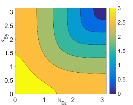
(b)

(c)

Figure 2: Isofrequency contours of first band surface $\omega/c_{0}$ for configurations in Fig. 1.

Next, we determine the conditions and asymptotic behavior of a band that emerges from the $M$ point at low frequencies. As before, we derive asymptotic forms for the $S_{l}^{\mathrm{Y}}$ sums near $M$ (see Supplemental Material sup ) and assume $\omega_{\mathrm{B}}=\alpha^{\prime}k_{\mathrm{B}}^{\prime}$, where $\alpha^{\prime}$ is real and positive-valued, $\mathbf{k}_{\mathrm{B}}^{\prime}=\mathbf{k}_{\mathrm{B}}-\mathbf{M}$ and $\mathbf{M}=(\pi/a,\pi/a)$. This assumption yields series coefficients for $S_{l}^{\mathrm{Y}}$ in $\omega_{\mathrm{B}}$ (given in Supplemental Material sup ). Substituting these expansions for $S_{l}^{\mathrm{Y}}$ and $N_{m}$ into (2), the zero determinant condition is satisfied to the lowest orders when

$$\varepsilon_{\mathrm{c}}=-\varepsilon_{\mathrm{b}},$$ (4)

and for $\alpha^{\prime}$ such that

$$\omega_{\mathrm{B}}=\left\{\frac{1}{8\pi^{2}}\left|64\pi^{4}\mathrm{e}^{4\mathrm{i}\theta_{\mathrm{B}}^{\prime}}+\Gamma(\tfrac{1}{4})^{8}\right|^{1/2}\phantom{\left[\varepsilon_{\mathrm{b}}\mu_{\mathrm{c}}+2\varepsilon_{\mathrm{b}}\mu_{\mathrm{b}}\log\left(\frac{16\pi^{2}}{f\Gamma(\tfrac{1}{4})^{4}}\right)\right]^{-1/2}}\right.\\ \left.\times\left[\varepsilon_{\mathrm{b}}\mu_{\mathrm{c}}+2\varepsilon_{\mathrm{b}}\mu_{\mathrm{b}}\log\left(\frac{16\pi^{2}}{f\Gamma(\tfrac{1}{4})^{4}}\right)\right]^{-1/2}\right\}k_{\mathrm{B}}^{\prime},$$ (5)

where $\Gamma(z)$ is the Gamma function. That is, a band surface is supported from $M$ at low frequencies provided (4) and $\alpha^{\prime}>0$ are satisfied. The condition $\varepsilon_{\mathrm{c}}=-\varepsilon_{\mathrm{b}}$ corresponds to an anomalous resonance in quasistatic problems Nicorovici et al. (1994, 2007) (discussed below).

Likewise, for the $X$ point at low frequencies, having derived asymptotic forms for the $S_{l}^{\mathrm{Y}}$ sums near $X$ (see Supplemental Material sup ) we assume that $\omega_{\mathrm{B}}=\alpha^{\prime\prime}k_{\mathrm{B}}^{\prime\prime}$, where $\alpha^{\prime\prime}$ is real and positive-valued, $\mathbf{k}_{\mathrm{B}}^{\prime\prime}=\mathbf{k}_{\mathrm{B}}-\mathbf{X}$, and $\mathbf{X}=(\pi/a,0)$. Substituting the resulting expansions for $S_{l}^{\mathrm{Y}}$, and $N_{m}$, into (2), the zero determinant condition is satisfied to leading order when

$$\varepsilon_{\mathrm{c}}=\left(\frac{\zeta-16\pi^{2}}{\zeta+16\pi^{2}}\right)\varepsilon_{\mathrm{b}},$$ (6)

where $\zeta=\Gamma(\tfrac{1}{4})^{4}f$. At the next order, provided

$$\mu_{\mathrm{c}}=\left(\frac{\zeta(\zeta-64\pi^{2})+512\pi^{4}\log\left({\zeta}/{(32\pi^{2})}\right)}{(\zeta-16\pi^{2})^{2}}\right)\mu_{\mathrm{b}},$$ (7)

then we obtain the low-frequency dispersion relation

$$\omega_{\mathrm{B}}=\left\{\frac{\left(16\Gamma(\tfrac{1}{4})^{4}\pi^{2}+64\pi^{4}\mathrm{e}^{2\mathrm{i}\theta_{\mathrm{B}}^{{\prime\prime}}}-\Gamma(\tfrac{1}{4})^{8}\mathrm{e}^{-2\mathrm{i}\theta_{\mathrm{B}}^{{\prime\prime}}}\right)}{16\Gamma(\tfrac{1}{4})^{4}\pi^{2}\varepsilon_{\mathrm{b}}\mu_{\mathrm{b}}}\right\}^{1/2}k_{\mathrm{B}}^{\prime\prime}.$$ (8a)

However, the slope in (8a) is only real-valued along $$\Gamma X XM \omega_{\mathrm{B}}^{2}=\alpha_{\mathrm{x}}^{\prime\prime}k_{\mathrm{B}\mathrm{x}}^{{\prime\prime}2}+\alpha_{\mathrm{y}}^{\prime\prime}k_{\mathrm{B}\mathrm{y}}^{{\prime\prime}2}$$ and . Numerical investigations confirm elliptical contours at low frequencies; interpolating between these paths with the ansatz we obtain

$$\omega_{\mathrm{B}}^{2}=\left(\frac{16\Gamma(\tfrac{1}{4})^{4}\pi^{2}+64\pi^{4}-\Gamma(\tfrac{1}{4})^{8}}{16\Gamma(\tfrac{1}{4})^{4}\pi^{2}\varepsilon_{\mathrm{b}}\mu_{\mathrm{b}}}\right)k_{\mathrm{B}\mathrm{x}}^{{\prime\prime}2}\\ +\left(\frac{16\Gamma(\tfrac{1}{4})^{4}\pi^{2}-64\pi^{4}+\Gamma(\tfrac{1}{4})^{8}}{16\Gamma(\tfrac{1}{4})^{4}\pi^{2}\varepsilon_{\mathrm{b}}\mu_{\mathrm{b}}}\right)k_{\mathrm{B}\mathrm{y}}^{{\prime\prime}2},$$ (8b)

for the first band surface as $$\omega_{\mathrm{B}}\rightarrow 0 \mathbf{k}_{\mathrm{B}}\rightarrow X$$ and as .

Hence, a band surface is supported from $X$ at low frequencies provided (6), (7), and $\varepsilon_{\mathrm{b}}\mu_{\mathrm{b}}>0$ are satisfied. In (6), the proportionality factor is negative-valued for $f\lesssim 0.914$, and the proportionality factor in (7) is negative-valued for all $f$, demonstrating that highly restrictive sign-changing conditions must be satisfied in both $\varepsilon_{\mathrm{r}}$ and $\mu_{\mathrm{r}}$ so that the first band emerges from $X$. The number of conditions for each high-symmetry Bloch coordinate is entirely due to the different asymptotic behaviors of $S_{l}^{\mathrm{Y}}$. For arbitrary Bloch coordinate origin, we anticipate that the number of conditions will change significantly.

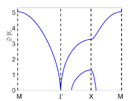
(a)

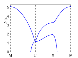
(b)

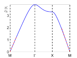
(c)

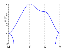
(d)

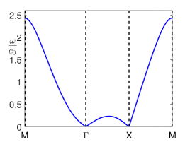
(e)

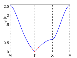
(f)

Figure 3: Band diagrams for square array of nonmagnetic cylinders ($\mu_{\mathrm{c}}=1$) embedded in air ($\varepsilon_{\mathrm{b}}=\mu_{\mathrm{b}}=1$) with LABEL:sub@fig:nonmagfigs1 $\varepsilon_{\mathrm{c}}=-0.55$, LABEL:sub@fig:nonmagfigs2 $\varepsilon_{\mathrm{c}}=-0.58$, LABEL:sub@fig:nonmagfigs3 $\varepsilon_{\mathrm{c}}=-1$, LABEL:sub@fig:nonmagfigs4 $\varepsilon_{\mathrm{c}}=-1.1$, LABEL:sub@fig:nonmagfigs5 $\varepsilon_{\mathrm{c}}\approx-1.896$, and LABEL:sub@fig:nonmagfigs6 $\varepsilon_{\mathrm{c}}=-2.1$. Dashed red lines in LABEL:sub@fig:nonmagfigs3 and LABEL:sub@fig:nonmagfigs6 are approximations (5) and (3), respectively. All figures use a dipolar approximation, lattice period $a=1$, and radius $a^{\prime}=0.3a$.

We now compare the asymptotic forms above against results from a fully numerical treatment of (2) within the dipole truncation. We begin by validating (3) for a regular photonic crystal; in Fig. 1a we present the band diagram of a representative crystal with $\varepsilon_{\mathrm{c}}=1$ and $\mu_{\mathrm{c}}=2$ embedded in air ($\varepsilon_{\mathrm{b}}=\mu_{\mathrm{c}}=1$). As expected, the first band emanates from the $\Gamma$ point, and (3) shows excellent agreement. In Fig. 1b we consider $\varepsilon_{\mathrm{c}}=-1$ and $\mu_{\mathrm{c}}=2$, where the first band emanates from the $M$ point as described by (5) at low frequencies, also with excellent agreement. In Fig. 1c we consider $\varepsilon_{\mathrm{c}}\approx-0.53$ and $\mu_{\mathrm{c}}\approx-10.22$ satisfying (6) and (7). Here, the slope differs along $\Gamma X$ and $XM$, demonstrating twofold symmetry as $\omega_{\mathrm{B}}\rightarrow 0$. The asymptotic estimate (8a) shows excellent agreement near $X$ at low frequencies. The diagram also possesses folded bands Chen et al. (2011) at high frequencies.

In Fig. 2 we present iso-frequency contours for the first band surfaces of the photonic crystals considered in Fig. 1, over a quarter of the first Brillouin zone. In Fig. 2a we see a cone ($\infty$-symmetric) as $\omega_{\mathrm{B}}\rightarrow 0$, whereas in Fig. 2b we observe fourfold symmetric contours, as expected from the $\mathrm{exp}(4\mathrm{i}\theta_{\mathrm{B}}^{\prime})$ dependence in (5). In Fig. 2c we see that the first band has twofold symmetric contours, as expected from (8b). These low-frequency symmetries contrast with the electronic band diagrams of graphene (and photonic analogues to graphene) where the high-energy band emanates from the $K$ point and about the Fermi energy $E_{F}$ as an ideal cone Reich et al. (2002); Zhang et al. (2005); Zandbergen and de Dood (2010).

Having numerically validated the $E$-$k$ relations (3), (5), and (8a), we now briefly demonstrate that magnetic constituents are not necessary to observe exotic low-frequency behaviors. Low-frequency descriptions of nonmagnetic photonic crystals emanating from $\Gamma$ and $M$ are obtained by the replacements $\mu_{\mathrm{b}},\mu_{\mathrm{c}}\mapsto 1$ in (3) and (5) above. This is despite the fact that the $N_{m}$ coefficients for nonmagnetic crystals exhibit different leading order behavior for small $\omega_{\mathrm{B}}$ (see Supplemental Material sup ). However, the new leading-order behavior of $N_{m}$ yields a nonmagnetic analogue to (7) of the form

$$\zeta+8\pi^{2}-16\pi^{2}\log\left(\zeta/(32\pi^{2})\right)=0,$$ (9)

which is not satisfied for any $f$. As such, low-frequency emanation from $X$ as $\omega_{\mathrm{B}}=\alpha^{\prime\prime}k_{\mathrm{B}}^{\prime\prime}$ or $\omega_{\mathrm{B}}^{2}=\alpha_{\mathrm{x}}^{\prime\prime}k_{\mathrm{B}\mathrm{x}}^{{\prime\prime}2}+\alpha_{\mathrm{y}}^{\prime\prime}k_{\mathrm{B}\mathrm{y}}^{{\prime\prime}2}$ is not supported for nonmagnetic crystals.

In Fig. 3 we present first band(s) for a selection of crystals comprising nonmagnetic cylinders ($\mu_{\mathrm{c}}=1$) in air, and describe their evolution as $\varepsilon_{\mathrm{c}}$ is varied from $0<\varepsilon_{\mathrm{c}}\leq-2.1$. For values $0>\varepsilon_{\mathrm{c}}\gtrsim-0.5274$ (6), a single first band emanates from the $\Gamma$ point, analogously to the $\Gamma$-emerging band in Fig. 3a. At $\varepsilon_{\mathrm{c}}\approx-0.5274$, a band emerges from the $X$ point, giving rise to two first band surfaces at low frequencies, as in Fig. 3a. This $X$-emergent surface eventually forms a double degeneracy at the $\Gamma$ point at $\varepsilon_{\mathrm{c}}\approx-0.56$, and thereafter, as shown in Fig. 3b, becomes the first band surface, pushing the existing $\Gamma$ centered band to higher frequencies. As we proceed in $\varepsilon_{\mathrm{c}}$, the origin of the first band travels along the $\Gamma M$ and $\Gamma X$ symmetry planes to the $M$ point at $\varepsilon_{\mathrm{c}}=-1$ (the anomalous resonance condition), as shown in Fig. 3c. Thereafter, a new first band emerges at the $M$ point whose origins move along high symmetry planes towards the $\Gamma$ point. At the same time, this emergent band pushes the existing $M$ centered band to higher frequencies. Both of these behaviors are demonstrated in Fig. 3d. The new first band eventually takes the form given in Fig. 3e where it emanates from both the $\Gamma$ and $X$ points simultaneously at $\varepsilon_{\mathrm{c}}=(\zeta+16\pi^{2})/(\zeta-16\pi^{2})\approx-1.896$. As we proceed in $\varepsilon_{\mathrm{c}}$, the first eigenfrequency at $X$ becomes nonzero and the first band emanates from the $\Gamma$ point alone, as demonstrated by Fig. 3f. Undoubtedly further behaviors are observed beyond $\varepsilon_{\mathrm{b}}<-2.1$, however, this falls outside the scope of the present work. Note that in Figs. 3c and 3f the dipolar approximations (5) and (3) are superposed, respectively, and show excellent agreement at low frequencies. The examples above, in consideration with (9), emphasize that the absence of a band from a single Bloch coordinate does not preclude the emergence of bands from multiple Bloch coordinates simultaneously; this observation has important implications for determining the existence of band gaps at low frequencies. We emphasize that the band structure smoothly transitions between the examples shown above.

In summary, we have determined new low-frequency $E$-$k$ relations for photons in 2D photonic crystals. These relations, and the conditions for their existence, are given explicitly for first bands with origins at the $\Gamma$, $X$, and $M$ points of a square lattice. In general, we have found that sign changes in the properties of the constituents are required for the first band to originate from coordinates away from $\Gamma$ at low frequencies. We have also demonstrated that photonic crystals can possess low-frequency $E$-$k$ relations with origins at one or more arbitrary Bloch coordinates. Given that all conventional photonic crystals possess either a low-frequency band gap or a band surface emanating from $\Gamma$, this work has significant implications for the homogenization of periodic media, theoretical descriptions of light propagation in complex media, as well as future photonic crystal designs. In the latter case, the closed-form conditions we obtain represent a powerful design tool for determining filling fractions and background materials for a given cylinder material, and vice versa. However, an important consequence of the $M$-point condition coinciding with the anomalous resonance condition is that the slope of the $M$-emerging band (5) is not necessarily accurate beyond a dipolar truncation; further investigations are required to accurately determine behaviors near resonance (see Supplemental Material sup ). Preliminary results for hexagonal lattices at the anomalous resonance reveal a band surface emerging from the $K$ point, implying that the first band originates from the furthest edge of the irreducible Brillouin zone when on resonance. Away from the anomalous resonance condition, we believe that experimental validation is feasible for the crystals we describe, as all emergence conditions (i.e., (6) and (7)) are valid for complex-valued $\varepsilon_{\mathrm{b}}$ and $\mu_{\mathrm{b}}$. When $\varepsilon_{\mathrm{b}}$ and $\mu_{\mathrm{b}}$ possess moderate loss, and $\varepsilon_{\mathrm{c}}$ and $\mu_{\mathrm{c}}$ satisfy the necessary emergence conditions, we find the band diagrams to be unchanged (see Supplemental Material sup ). A natural next step for this work is 1D and 3D photonic structures; 2D photonic crystals were only chosen for analytical convenience. Finally, we emphasize that our approach extends readily to phononic and other systems.

M.J.A.S. acknowledges discussions with R.C. McPhedran, S. Guenneau, R.V. Craster, support from the ERC (279673), and support from the EPSRC (EP/L018039/1).

I Supplemental Material for “Violating the energy-momentum proportionality of photonic crystals in the low-frequency limit”

II Extended problem formulation

We begin by considering the time-harmonic form of the source-free Maxwell equations, in a non-dispersive and lossless system. The domain comprises a two-dimensional array of infinitely extending isotropic cylinders that are periodically positioned at the coordinates of a square lattice in the $(x,y)$ plane and embedded in an isotropic background material. That is, we examine the band structure of the Maxwell equations

$$\nabla\times\mathbf{H}=-\mathrm{i}\omega\mathbf{D}, \quad\nabla\times\mathbf{E}=\mathrm{i}\omega\mathbf{B},$$

$$\nabla\cdot\mathbf{D}=0, \quad\nabla\cdot\mathbf{B}=0,$$ (10)

having assumed that fields possess the dependence $\mathrm{exp}(-\mathrm{i}\omega t)$. We then assume the linear constitutive relations

$$\mathbf{D}=\varepsilon_{0}\varepsilon_{\mathrm{r}}\mathbf{E},\quad\mbox{ and }\quad\mathbf{B}=\mu_{0}\mu_{\mathrm{r}}\mathbf{H},$$ (11)

where the relative permittivity and permeability tensors take the scalar values

$$\varepsilon_{\mathrm{r}}=\left\{\begin{array}[]{ll}\varepsilon_{\mathrm{c}}&\mbox{for}\,\mathbf{x}\in\Omega_{\mathrm{c}}\\ \varepsilon_{\mathrm{b}}&\mbox{for}\,\mathbf{x}\in\Omega_{\mathrm{b}}\end{array}\right.,\quad\mu_{\mathrm{r}}=\left\{\begin{array}[]{ll}\mu_{\mathrm{c}}&\mbox{for}\,\mathbf{x}\in\Omega_{\mathrm{c}}\\ \mu_{\mathrm{b}}&\mbox{for}\,\mathbf{x}\in\Omega_{\mathrm{b}}\end{array}\right.,$$ (12)

where $\Omega_{\mathrm{c}}$ denotes the region inside the cylinder (of radius $r=a^{\prime}$) positioned in the centre of the fundamental unit cell $\Omega_{\mathrm{WSC}}$, and $\Omega_{\mathrm{b}}$ represents the remainder of the unit cell (i.e., $\Omega_{\mathrm{b}}=\Omega_{\mathrm{WSC}}\backslash\Omega_{\mathrm{c}}$). Substituting the constitutive relations (11) into the Maxwell system (II) admits the vector wave equation

$$\nabla\times\varepsilon_{\mathrm{r}}^{-1}\nabla\times\mathbf{H}-\omega^{2}c_{0}^{-2}\mu_{\mathrm{r}}\mathbf{H}=0.$$ (13)

We then impose that all electromagnetic fields have the dependence $\mathrm{exp}(\mathrm{i}k_{z}z)$ and that wave propagation in the direction of the fibres is forbidden, i.e. $k_{z}=0$. Subsequently, the Bloch vector takes the form $\mathbf{k}=(k_{x},k_{y},0)$ where we introduce $\mathbf{k}_{\mathrm{B}}=(k_{x},k_{y})$ as the in-plane Bloch wave vector. This restriction on the wave vector permits a decomposition of the Maxwell wave equation (13) above into two decoupled scalar problems for the two orthogonal polarisation states; the first with the electric field $\mathbf{E}$ polarised in the direction $z$ (along the cylinders), and the second with the magnetic field $\mathbf{H}$ polarised in the direction $z$.

In this work, we examine the latter polarisation problem and subsequently the Maxwell wave equation (13) reduces to the study of the two-dimensional Helmholtz equation

$$\nabla_{\perp}\cdot\left(\varepsilon_{\mathrm{r}}^{-1}\nabla_{\perp}H_{\mathrm{z}}\right)+\omega^{2}c_{0}^{-2}\mu_{\mathrm{r}}H_{\mathrm{z}}=0,$$ (14)

where $\nabla_{\perp}\equiv(\partial_{\mathrm{x}},\partial_{\mathrm{y}})$ denotes the in-plane gradient, $\omega$ denotes the angular frequency, and $c_{0}$ is the speed of light in vacuum. Similarly, the electromagnetic continuity conditions at the edges of the cylinders take the form

$$\left(H_{\mathrm{z}}^{\mathrm{c}}-H_{\mathrm{z}}^{\mathrm{b}}\right)\big{|}_{r=a^{\prime}}=0,\quad\left(\varepsilon_{\mathrm{c}}^{-1}\partial_{r}H_{\mathrm{z}}^{\mathrm{c}}-\varepsilon_{\mathrm{b}}^{-1}\partial_{r}H_{\mathrm{z}}^{\mathrm{b}}\right)\big{|}_{r=a^{\prime}}=0,$$ (15a)

corresponding to continuity of $$H_{z} E_{\theta}$$ and at the boundary, respectively. Additionally, we impose the Floquet–Bloch conditions

$$H_{\mathrm{z}}(\mathbf{x}+\mathbf{R}_{p})=H_{\mathrm{z}}(\mathbf{x})\mathrm{e}^{\mathrm{i}\mathbf{k}_{\mathrm{B}}\cdot\mathbf{R}_{p}},$$ (15b)

where $\mathbf{R}_{p}=(ma,na)$ for $m,n\in\mathbb{Z}$ is the real-lattice vector for a square lattice of period $a$, where $p$ is multi-index notation for the pair $(m,n)$. The system for the $E_{\mathrm{z}}$ polarised field is given by exchanging $\varepsilon_{\mathrm{r}}$ and $\mu_{\mathrm{r}}$ in the above, and subsequently all band diagrams shown are thus also attainable under the $E_{\mathrm{z}}$ polarisation. The general solution to the homogeneous two-dimensional Helmholtz equation (14) is well-known and takes the form

$$H_{\mathrm{z}}=\left\{\begin{array}[]{lc}H_{\mathrm{z}}^{\mathrm{b}},&\mbox{for}\,\mathbf{x}\in\Omega_{\mathrm{b}},\\ H_{\mathrm{z}}^{\mathrm{c}},&\mbox{for}\,\mathbf{x}\in\Omega_{\mathrm{c}},\end{array}\right.$$ (16)

where

$$H_{\mathrm{z}}^{\mathrm{b}} =\sum\limits_{m=-\infty}^{\infty}\left[\mathcal{A}_{m}J_{m}(\omega_{\mathrm{B}}n_{\mathrm{b}}r)+\mathcal{B}_{m}Y_{m}(\omega_{\mathrm{B}}n_{\mathrm{b}}r)\right]\mathrm{e}^{\mathrm{i}m\theta},$$ (17a)

$$H_{\mathrm{z}}^{\mathrm{c}} =\sum\limits_{m=-\infty}^{\infty}\mathcal{C}_{m}J_{m}(\omega_{\mathrm{B}}n_{\mathrm{c}}r)\,\mathrm{e}^{\mathrm{i}m\theta},$$ (17b)

with $(r,\theta)$ denoting polar coordinates in the $(x,y)$ plane, $\omega_{\mathrm{B}}=\omega/c_{0}$, $n_{\mathrm{c}}=\sqrt{\varepsilon_{\mathrm{c}}}\sqrt{\mu_{\mathrm{c}}}$, and $n_{\mathrm{b}}=\sqrt{\varepsilon_{\mathrm{b}}}\sqrt{\mu_{\mathrm{b}}}$. Note that in this work, we choose the positive branch of the square root function as the principal root and that $\sqrt{\varepsilon}\sqrt{\mu}\neq\sqrt{\varepsilon\mu}$ in general; such a result only holds when both parameters are positive-valued. From our definition of $n$ above, we observe that both $\varepsilon$ and $\mu$ must be negative-valued in order to obtain a negative-index material ($n<0$). The functions $J_{m}(z)$ and $Y_{m}(z)$ denote Bessel functions of the first and second kind. Substituting these general solutions (17) into the boundary conditions (15a) we obtain

$$\mathcal{C}_{m}=\frac{\mathcal{A}_{m}J_{m}(\omega_{\mathrm{B}}n_{\mathrm{b}}a^{\prime})+\mathcal{B}_{m}Y_{m}(\omega_{\mathrm{B}}n_{\mathrm{b}}a^{\prime})}{J_{m}(\omega_{\mathrm{B}}n_{\mathrm{c}}a^{\prime})},$$ (18a)

and

$$\mathcal{A}_{m}=-N_{m}\mathcal{B}_{m},$$ (18b)

where

$$N_{m}=\frac{Z_{\mathrm{b}}^{-1}Y_{m}(n_{\mathrm{b}}\omega_{\mathrm{B}}a^{\prime})\partial_{r}J_{m}(r)\big{|}_{r=n_{\mathrm{c}}\omega_{\mathrm{B}}a^{\prime}}-Z_{\mathrm{c}}^{-1}J_{m}(n_{\mathrm{c}}\omega_{\mathrm{B}}a^{\prime})\partial_{r}Y_{m}(r)\big{|}_{r=n_{\mathrm{b}}\omega_{\mathrm{B}}a^{\prime}}}{Z_{\mathrm{b}}^{-1}J_{m}(n_{\mathrm{b}}\omega_{\mathrm{B}}a^{\prime})\partial_{r}J_{m}(r)\big{|}_{r=n_{\mathrm{c}}\omega_{\mathrm{B}}a^{\prime}}-Z_{\mathrm{c}}^{-1}J_{m}(n_{\mathrm{c}}\omega_{\mathrm{B}}a^{\prime})\partial_{r}J_{m}(r)\big{|}_{r=n_{\mathrm{b}}\omega_{\mathrm{B}}a^{\prime}}},$$ (18c)

having introduced the impedances $Z_{\mathrm{c}}=\sqrt{\mu_{\mathrm{c}}}/\sqrt{\varepsilon_{\mathrm{c}}}$ and $Z_{\mathrm{b}}=\sqrt{\mu_{\mathrm{b}}}/\sqrt{\varepsilon_{\mathrm{b}}}$. In the presence of an incident plane wave, we determine the scattered fields from all other cylinders in the array (i.e., the multiple scattering contribution) using Green’s second identity, admitting the Rayleigh identity Movchan et al. (2002)

$$\mathcal{A}_{l}=\sum_{m=-\infty}^{\infty}(-1)^{l+m}S_{m-l}^{\mathrm{Y}}\mathcal{B}_{m},$$ (19)

where $S_{m}^{\mathrm{Y}}$ denote lattice sums (defined in Section VI) and we have omitted the incident field as we seek the Bloch modes of the structure. Substituting (18b) into (19) above we obtain the system

$$N_{l}\mathcal{B}_{l}+\sum_{m=-\infty}^{\infty}(-1)^{l+m}S_{m-l}^{\mathrm{Y}}\mathcal{B}_{m}=0,$$ (20)

whose vanishing determinant gives the dispersion equation for the homogeneous periodic problem. To obtain a numerically tractable form of (20), it is necessary to truncate parameters, i.e. to evaluate (20) for $l,m=-L,\ldots,L$. For conventional photonic crystals, the convergence of the band surfaces improves with larger truncation values $L$. However, at low frequencies a monopole $(L=0)$ or dipole truncation ($L=1$) is regarded as a good approximation for the fully converged dispersion equation.

III Asymptotic analysis of dispersion equation

In the preceding section we determined the form of the dispersion equation (20) for a two-dimensional photonic crystal of infinitely extending cylinders, which to monopolar order ($L=0$) takes the form

$$N_{0}+S_{0}^{\mathrm{Y}}=0,$$ (21)

and to dipolar order ($L=1$) takes the form

$$\left(N_{0}+S_{0}^{\mathrm{Y}}\right)\left(\left[N_{1}+S_{0}^{\mathrm{Y}}\right]^{2}-\left|S_{2}^{\mathrm{Y}}\right|^{2}\right)+\left(S_{1}^{\mathrm{Y}}\right)^{2}\left[S_{2}^{\mathrm{Y}}\right]^{\ast}-2\left|S_{1}^{\mathrm{Y}}\right|^{2}\left(N_{1}+S_{0}^{\mathrm{Y}}\right)+\left(\left[S_{1}^{\mathrm{Y}}\right]^{\ast}\right)^{2}S_{2}^{\mathrm{Y}}=0,$$ (22)

where we have used the identities $N_{-m}=N_{m}$ and $S_{-l}^{\mathrm{Y}}=\left[S_{l}^{\mathrm{Y}}\right]^{\ast}$, where $\ast$ denotes complex conjugation Movchan et al. (2002). In this section, we obtain conditions necessary for the existence of band surfaces, through a close examination of (21) and (22) in the low-frequency regime.

III.1 Asymptotic behaviour of dispersion relations near the $\Gamma$ point

We begin by evaluating asymptotic expressions for the scattering coefficients $N_{m}$ defined in (18c) in the limit as $\omega_{\mathrm{B}}=\omega/c_{0}\rightarrow 0$. These terms exhibit the leading order behaviour

$$\lim_{\omega_{\mathrm{B}}\rightarrow 0}N_{m}=\left\{\begin{array}[]{ll}O(\omega_{\mathrm{B}}^{-2})&\mbox{ for }m=0\\ O(\omega_{\mathrm{B}}^{-2m})&\mbox{ for }m>0\\ \end{array}\right.,$$ (23)

and subsequently we write

$$\lim_{{\omega_{\mathrm{B}}}\rightarrow 0}\left\{N_{0}\right\}\approx\sum_{m=-2}^{\infty}D_{m}\omega_{\mathrm{B}}^{m},\quad\mbox{ and }\quad\lim_{{\omega_{\mathrm{B}}}\rightarrow 0}\left\{N_{1}\right\}\approx\sum_{m=-2}^{\infty}E_{m}\omega_{\mathrm{B}}^{m},$$ (24a)

where the first few terms of these series are given by

$$D_{-2} =\frac{4}{\pi a^{\prime 2}\varepsilon_{\mathrm{b}}}\frac{1}{\mu_{\mathrm{c}}-\mu_{\mathrm{b}}},$$ (25a)

$$D_{0} =\frac{(4\mu_{\mathrm{c}}-3\mu_{\mathrm{b}})\varepsilon_{\mathrm{b}}\mu_{\mathrm{b}}-\mu_{\mathrm{c}}^{2}\varepsilon_{\mathrm{c}}}{2\pi\varepsilon_{\mathrm{b}}(\mu_{\mathrm{b}}-\mu_{\mathrm{c}})^{2}}+\frac{2}{\pi}\bigg{[}\gamma_{\mathrm{e}}+\log(\omega_{\mathrm{B}})\bigg{]}+\frac{1}{\pi}\log\left(\frac{a^{\prime 2}\varepsilon_{\mathrm{b}}\mu_{\mathrm{b}}}{4}\right),$$ (25b)

$$E_{-2} =\frac{4}{\pi a^{\prime 2}\varepsilon_{\mathrm{b}}\mu_{\mathrm{b}}}\frac{\varepsilon_{\mathrm{c}}+\varepsilon_{\mathrm{b}}}{\varepsilon_{\mathrm{c}}-\varepsilon_{\mathrm{b}}},$$ (25c)

$$E_{0} =\frac{\mu_{\mathrm{b}}(\varepsilon_{\mathrm{b}}+\varepsilon_{\mathrm{c}})(5\varepsilon_{\mathrm{c}}-3\varepsilon_{\mathrm{b}})-4\mu_{\mathrm{c}}\varepsilon_{\mathrm{c}}^{2}}{2\pi\mu_{\mathrm{b}}(\varepsilon_{\mathrm{b}}-\varepsilon_{\mathrm{c}})^{2}}+\frac{2}{\pi}\bigg{[}\gamma_{\mathrm{e}}+\log(\omega_{\mathrm{B}})\bigg{]}+\frac{1}{\pi}\log\left(\frac{a^{\prime 2}{\varepsilon_{\mathrm{b}}}{\mu_{\mathrm{b}}}}{4}\right),$$ (25d)

and $\gamma_{\mathrm{e}}\approx 0.577215\ldots$ denotes the Euler–Mascheroni constant.

Next we consider the leading-order behaviours of the $S_{l}^{\mathrm{Y}}$ terms present in (21) and (22). Semi-analytical representations for these sums were previously determined by McPhedran et al. (1996); Movchan et al. (2002), using numerical estimates for certain terms. Using the approach in Chen et al. (2018) (details in Section VI) we obtain the fully closed forms

$$\lim_{k_{\mathrm{B}}\rightarrow 0}\lim_{\omega_{\mathrm{B}}\rightarrow 0}S_{0}^{Y} \approx-\frac{4}{a^{2}}\frac{1}{k_{\mathrm{B}}^{2}-(n_{\mathrm{b}}\omega_{\mathrm{B}})^{2}}-\frac{2}{\pi}\log(n_{\mathrm{b}}\omega_{\mathrm{B}})-\frac{2\gamma_{\mathrm{e}}}{\pi}-\frac{1}{\pi}\log\left(\frac{a^{2}\pi}{\Gamma(\tfrac{1}{4})^{4}}\right),$$ (26a)

$$\lim_{k_{\mathrm{B}}\rightarrow 0}\lim_{\omega_{\mathrm{B}}\rightarrow 0}S_{1}^{Y} \approx-\frac{4\mathrm{i}}{a^{2}}\frac{k_{\mathrm{B}}}{n_{\mathrm{b}}\omega_{\mathrm{B}}}\frac{1}{k_{\mathrm{B}}^{2}-(n_{\mathrm{b}}\omega_{\mathrm{B}})^{2}}\mathrm{e}^{\mathrm{i}\theta_{\mathrm{B}}}+\frac{\mathrm{i}}{\pi}\frac{k_{\mathrm{B}}}{n_{\mathrm{b}}\omega_{\mathrm{B}}}\mathrm{e}^{\mathrm{i}\theta_{\mathrm{B}}},$$ (26b)

$$\lim_{k_{\mathrm{B}}\rightarrow 0}\lim_{\omega_{\mathrm{B}}\rightarrow 0}S_{2}^{Y} \approx\frac{4}{a^{2}}\frac{k_{\mathrm{B}}^{2}}{(n_{\mathrm{b}}\omega_{\mathrm{B}})^{2}}\frac{1}{k_{\mathrm{B}}^{2}-(n_{\mathrm{b}}\omega_{\mathrm{B}})^{2}}\mathrm{e}^{2\mathrm{i}\theta_{\mathrm{B}}}+\frac{k_{\mathrm{B}}^{2}}{(n_{\mathrm{b}}\omega_{\mathrm{B}})^{2}}\left[\left(\frac{\Gamma(\tfrac{1}{4})^{8}}{384\pi^{5}}\right)\mathrm{e}^{-2\mathrm{i}\theta_{\mathrm{B}}}-\frac{1}{2\pi}\mathrm{e}^{2\mathrm{i}\theta_{\mathrm{B}}}\right],$$ (26c)

where $(k_{\mathrm{B}},\theta_{\mathrm{B}})$ is the polar representation of the Bloch vector $\mathbf{k}_{\mathrm{B}}$, and $\Gamma(z)$ is the Gamma function. We now assume that a band surface emanates from the $\Gamma$ point at low frequencies in the form $\omega_{\mathrm{B}}=\alpha k_{\mathrm{B}}$, where $\alpha$ is real and positive-valued, and substitute this into (26) to obtain

$$\lim_{k_{\mathrm{B}}\rightarrow 0}\lim_{\omega_{\mathrm{B}}\rightarrow 0}S_{l}^{Y}(\omega_{\mathrm{B}},\mathbf{k}_{\mathrm{B}};n_{\mathrm{b}})\sim O(\omega_{\mathrm{B}}^{-2}),$$ (27)

for $l=0,1,2,$ and where we treat $\log(\omega_{\mathrm{B}})$ terms as $O(\omega_{\mathrm{B}}^{0})$. Subsequently, we expand the lattice sums in the form

$$\lim_{k_{\mathrm{B}}\rightarrow 0}\lim_{\omega_{\mathrm{B}}\rightarrow 0}\left\{S_{0}^{Y}\right\}\approx\sum_{m=-2}^{\infty}A_{m}\omega_{\mathrm{B}}^{m},\qquad\lim_{k_{\mathrm{B}}\rightarrow 0}\lim_{\omega_{\mathrm{B}}\rightarrow 0}\left\{S_{1}^{Y}\right\}\approx\sum_{m=-2}^{\infty}B_{m}\omega_{\mathrm{B}}^{m},\quad\mbox{ and }\quad\lim_{k_{\mathrm{B}}\rightarrow 0}\lim_{\omega_{\mathrm{B}}\rightarrow 0}\left\{S_{2}^{Y}\right\}\approx\sum_{m=-2}^{\infty}C_{m}\omega_{\mathrm{B}}^{m},$$ (28)

where summation is made over non-zero orders, all of which are even due to symmetry. Substituting (24a) and (28) into the monopolar dispersion equation (21) and collecting terms in advancing orders of $\omega_{\mathrm{B}}$ reveals a hierarchy of equations describing the leading-order behaviour of the dispersion relation at low frequencies and the conditions necessary for the existence of the band.

The first non-vanishing order for the monopolar dispersion equation (21) is given by

$$O(\omega_{\mathrm{B}}^{-2}):\quad A_{-2}+D_{-2}=0,$$ (29)

where (24a) and (26) admit the dispersion relation

$$\omega_{\mathrm{B}}=\left\{\frac{1}{{\varepsilon_{\mathrm{b}}\left[\mu_{\mathrm{b}}+f(\mu_{\mathrm{c}}-\mu_{\mathrm{b}})\right]}}\right\}^{1/2}k_{\mathrm{B}},$$ (30)

Subsequently, provided $\varepsilon_{\mathrm{b}}\mu_{\mathrm{b}}+f\varepsilon_{\mathrm{b}}(\mu_{\mathrm{c}}-\mu_{\mathrm{b}})>0$, a low-frequency band surface emanates from the $\Gamma$ point within a monopolar approximation.

Proceeding to the dipolar truncation (22), the first non-vanishing order is

$$O(\omega_{\mathrm{B}}^{-6}):\quad(A_{-2})^{3}+(A_{-2})^{2}(D_{-2}+2E_{-2})+A_{-2}\left[(E_{-2})^{2}-|C_{-2}|^{2}+2D_{-2}E_{-2}-2|B_{-2}|^{2}\right]\\ +(C_{-2})^{\ast}(B_{-2})^{2}+\left[(B_{-2})^{\ast}\right]^{2}C_{-2}-2|B_{-2}|^{2}E_{-2}+D_{-2}\left[(E_{-2})^{2}-|C_{-2}|^{2}\right]=0,$$ (31)

which gives the low-frequency dispersion relation

$$\omega_{\mathrm{B}}=\left\{\frac{{(\varepsilon_{\mathrm{b}}+\varepsilon_{\mathrm{c}})+f(\varepsilon_{\mathrm{b}}-\varepsilon_{\mathrm{c}})}}{{\left[\varepsilon_{\mathrm{b}}\mu_{\mathrm{b}}+f\varepsilon_{\mathrm{b}}(\mu_{\mathrm{c}}-\mu_{\mathrm{b}})\right]}{\left[(\varepsilon_{\mathrm{b}}+\varepsilon_{\mathrm{c}})-f(\varepsilon_{\mathrm{b}}-\varepsilon_{\mathrm{c}})\right]}}\right\}^{1/2}k_{\mathrm{B}},$$ (32)

where $f=\pi a^{\prime 2}/a^{2}$ is the filling fraction, provided

$$\frac{{(\varepsilon_{\mathrm{b}}+\varepsilon_{\mathrm{c}})+f(\varepsilon_{\mathrm{b}}-\varepsilon_{\mathrm{c}})}}{{\left[\varepsilon_{\mathrm{b}}\mu_{\mathrm{b}}+f\varepsilon_{\mathrm{b}}(\mu_{\mathrm{c}}-\mu_{\mathrm{b}})\right]}{\left[(\varepsilon_{\mathrm{b}}+\varepsilon_{\mathrm{c}})-f(\varepsilon_{\mathrm{b}}-\varepsilon_{\mathrm{c}})\right]}}>0.$$ (33)

Note that (30) is recovered under the substitution $\varepsilon_{\mathrm{c}}=\varepsilon_{\mathrm{b}}$ in (32) above, and that an effective refractive index is readily obtained via $n_{\mathrm{eff}}=1/\alpha$. In this setting, the expressions for the effective permittivity and permeability are decoupled, motivating the representations

$$\varepsilon_{\mathrm{eff}}=\varepsilon_{\mathrm{b}}\left(\frac{(\varepsilon_{\mathrm{b}}+\varepsilon_{\mathrm{c}})-f(\varepsilon_{\mathrm{b}}-\varepsilon_{\mathrm{c}})}{(\varepsilon_{\mathrm{b}}+\varepsilon_{\mathrm{c}})+f(\varepsilon_{\mathrm{b}}-\varepsilon_{\mathrm{c}})}\right)=\varepsilon_{\mathrm{b}}+\frac{2\varepsilon_{\mathrm{b}}(\varepsilon_{\mathrm{c}}-\varepsilon_{\mathrm{b}})f}{(\varepsilon_{\mathrm{c}}+\varepsilon_{\mathrm{b}})-(\varepsilon_{\mathrm{c}}-\varepsilon_{\mathrm{b}})f},\qquad\mu_{\mathrm{eff}}=\mu_{\mathrm{b}}+f(\mu_{\mathrm{c}}-\mu_{\mathrm{b}}).$$ (34)

Having determined the low-frequency dispersion relation in the vicinity of the $\Gamma$ point, we now consider the asymptotics of the dispersion relation both at low frequencies and in the vicinity of other high symmetry points.

III.2 Asymptotic behaviour of dispersion relations near the $M$ point

The asymptotic forms of the first few $S_{l}^{\mathrm{Y}}$ sums in the limit of vanishing frequency and in the vicinity of the $M$ point are given by

$$\lim_{k_{\mathrm{B}}\rightarrow M}\lim_{\omega_{\mathrm{B}}\rightarrow 0}\left\{S_{0}^{Y}\right\} \approx-\frac{2\gamma_{\mathrm{e}}}{\pi}-\frac{2}{\pi}\log\left(n_{\mathrm{b}}\omega_{\mathrm{B}}\right)-\frac{1}{\pi}\log\left(\frac{4a^{2}\pi}{\Gamma(\tfrac{1}{4})^{4}}\right),$$ (35a)

$$\lim_{k_{\mathrm{B}}\rightarrow M}\lim_{\omega_{\mathrm{B}}\rightarrow 0}\left\{S_{1}^{Y}\right\} \approx\frac{\mathrm{i}}{\pi}\frac{k_{\mathrm{B}}^{\prime}}{n_{\mathrm{b}}\omega_{\mathrm{B}}}\mathrm{e}^{\mathrm{i}\theta_{\mathrm{B}}^{\prime}},$$ (35b)

$$\lim_{k_{\mathrm{B}}\rightarrow M}\lim_{\omega_{\mathrm{B}}\rightarrow 0}\left\{S_{2}^{Y}\right\} \approx-\frac{k_{\mathrm{B}}^{\prime 2}}{(n_{\mathrm{b}}\omega_{\mathrm{B}})^{2}}\left[\frac{1}{\pi^{2}}\left(\frac{\Gamma(\tfrac{1}{4})^{8}}{128\pi^{3}}\right)\mathrm{e}^{-2\mathrm{i}\theta_{\mathrm{B}}^{\prime}}+\frac{1}{2\pi}\mathrm{e}^{2\mathrm{i}\theta_{\mathrm{B}}^{\prime}}\right],$$ (35c)

where $(k_{\mathrm{B}}^{\prime},\theta_{\mathrm{B}}^{\prime})$ is the polar representation of $\mathbf{k}_{\mathrm{B}}^{\prime}=\mathbf{k}_{\mathrm{B}}-\mathbf{M}$, with $\mathbf{M}=(\pi/a,\pi/a)$. A derivation of these expression is presented in Section VI. As in Section III.1 we now construct an ansatz assuming that a low frequency band surface emanates from the $M$ point in the form $\omega_{\mathrm{B}}=\alpha^{\prime}k_{\mathrm{B}}^{\prime}$, where $\alpha^{\prime}$ is real and positive-valued. From the lattice sum asymptotics in (35) this dependence yields

$$\lim_{k_{\mathrm{B}}\rightarrow M}\lim_{\omega_{\mathrm{B}}\rightarrow 0}S_{l}^{Y}(\omega_{\mathrm{B}},\mathbf{k}_{\mathrm{B}};n_{\mathrm{b}})\sim O(\omega_{\mathrm{B}}^{0}),$$ (36)

and so we introduce the expansions

$$\lim_{k_{\mathrm{B}}\rightarrow M}\lim_{\omega_{\mathrm{B}}\rightarrow 0}\left\{S_{0}^{Y}\right\}\approx\sum_{m=0}^{\infty}A_{m}^{\prime}\omega_{\mathrm{B}}^{m},\quad\lim_{k_{\mathrm{B}}\rightarrow M}\lim_{\omega_{\mathrm{B}}\rightarrow 0}\left\{S_{1}^{Y}\right\}\approx\sum_{m=0}^{\infty}B_{m}^{\prime}\omega_{\mathrm{B}}^{m},\quad\mbox{ and }\quad\lim_{k_{\mathrm{B}}\rightarrow M}\lim_{\omega_{\mathrm{B}}\rightarrow 0}\left\{S_{2}^{Y}\right\}\approx\sum_{m=0}^{\infty}C_{m}^{\prime}\omega_{\mathrm{B}}^{m},$$ (37)

where summation is made over even orders, as the odd orders remain identically zero. Next we substitute the expansion for $N_{0}$ in (24a) and $S_{0}^{\mathrm{Y}}$ in (37) into the monopolar dispersion equation (21) and collect terms in $\omega_{\mathrm{B}}$ to obtain a hierarchy of conditions. The first two of these equations are

$$O(\omega_{\mathrm{B}}^{-2}): \quad D_{-2}=0,$$ (38a)

$$O(\omega_{\mathrm{B}}^{0}): \quad D_{0}+A_{0}^{\prime}=0,$$ (38b)

where from (25a), it follows that the $O(\omega_{\mathrm{B}}^{-2})$ equation is never satisfied for finite permittivity and permeability values, and subsequently a band surface is not supported from the $M$ point at low frequencies within a monopolar approximation. This finding is consistent with the fact that a monopole field is symmetric and subsequently cannot satisfy quasi-periodic boundary conditions at the unit cell edges.

In contrast, from the dipolar dispersion equation (22) we obtain

$$O(\omega_{\mathrm{B}}^{-6}): \quad\left(E_{-2}\right)^{2}D_{-2}=0,$$ (39a)

$$O(\omega_{\mathrm{B}}^{-4}): \quad E_{-2}\left[(A_{0}^{\prime}+D_{0})E_{-2}+2(A_{0}^{\prime}+E_{0})D_{-2}\right]=0,$$ (39b)

$$O(\omega_{\mathrm{B}}^{-2}): \quad\begin{multlined}D_{-2}\left[(A_{0}^{\prime}+E_{0})^{2}-|C_{0}^{\prime}|^{2}\right]+(E_{-2})^{2}(A_{2}^{\prime}+D_{2})\\ +2E_{-2}\left[(A_{0}^{\prime})^{2}-|B_{0}^{\prime}|^{2}+A_{2}^{\prime}D_{-2}+D_{0}E_{0}+A_{0}^{\prime}(D_{0}+E_{0})+D_{-2}E_{2}\right]=0,\end{multlined}D_{-2}\left[(A_{0}^{\prime}+E_{0})^{2}-|C_{0}^{\prime}|^{2}\right]+(E_{-2})^{2}(A_{2}^{\prime}+D_{2})\\ +2E_{-2}\left[(A_{0}^{\prime})^{2}-|B_{0}^{\prime}|^{2}+A_{2}^{\prime}D_{-2}+D_{0}E_{0}+A_{0}^{\prime}(D_{0}+E_{0})+D_{-2}E_{2}\right]=0,$$ (39e)

where from inspection, the $O(\omega_{\mathrm{B}}^{-6})$ and $O(\omega_{\mathrm{B}}^{-4})$ equations are satisfied when $E_{-2}=0$, or $\varepsilon_{\mathrm{c}}=-\varepsilon_{\mathrm{b}}$ following (25c). Furthermore, the $O(\omega_{\mathrm{B}}^{-2})$ equation is simplified by the $E_{-2}=0$ requirement, reducing it to the form

$$O(\omega_{\mathrm{B}}^{-2}):\quad D_{-2}\left(A_{0}^{\prime}+E_{0}-|C_{0}^{\prime}|\right)\left(A_{0}^{\prime}+E_{0}+|C_{0}^{\prime}|\right)=0,$$ (40)

where $A_{0}^{\prime}+E_{0}+|C_{0}^{\prime}|=0$ ultimately gives the dispersion relation

$$\omega_{\mathrm{B}}=\left\{\frac{1}{8\pi^{2}}\left|64\pi^{4}\mathrm{e}^{4\mathrm{i}\theta_{\mathrm{B}}^{\prime}}+\Gamma(\tfrac{1}{4})^{8}\right|^{1/2}\left[\varepsilon_{\mathrm{b}}\mu_{\mathrm{c}}+2\varepsilon_{\mathrm{b}}\mu_{\mathrm{b}}\log\left(\frac{16\pi^{2}}{f\Gamma(\tfrac{1}{4})^{4}}\right)\right]^{-1/2}\right\}k_{\mathrm{B}}^{\prime}.$$ (41)

Thus within a dipolar approximation, a band surface is supported from the $M$ point at low frequencies (with a slope described by (41)) provided both

$$\varepsilon_{\mathrm{c}}=-\varepsilon_{\mathrm{b}},$$ (42a)

and

$$\mu_{\mathrm{c}}>\left[\log\left(\frac{f^{2}\Gamma(\tfrac{1}{4})^{8}}{2^{8}\pi^{4}}\right)\right]\mu_{\mathrm{b}},$$ (42b)

are satisfied, where the prefactor in (42b) is negative-valued for $0<f\lesssim 0.914$ (and for reference, $f=\pi/4\approx 0.785$ represents dense packing for a square array of cylinders). The expression (42b) follows from the condition that $\alpha$ must be real and positive-valued.

III.3 Asymptotic behaviour of dispersion relations near the $X$ point

The asymptotic forms of the first few $S_{l}^{\mathrm{Y}}$at both low frequencies and in the vicinity of the $X$ point are given by

$$\lim_{k_{\mathrm{B}}\rightarrow X}\lim_{\omega_{\mathrm{B}}\rightarrow 0}S_{0}^{Y} \approx-\frac{2\gamma_{\mathrm{e}}}{\pi}-\frac{2}{\pi}\log(n_{\mathrm{b}}\omega_{\mathrm{B}})-\frac{1}{\pi}\log\left(\frac{8a^{2}\pi}{\Gamma(\tfrac{1}{4})^{4}}\right),$$ (43a)

$$\lim_{k_{\mathrm{B}}\rightarrow X}\lim_{\omega_{\mathrm{B}}\rightarrow 0}S_{1}^{Y} \approx\frac{\mathrm{i}}{\pi}\frac{k_{\mathrm{B}}^{\prime\prime}}{n_{\mathrm{b}}\omega_{\mathrm{B}}}\left(\mathrm{e}^{\mathrm{i}\theta_{\mathrm{B}}^{\prime\prime}}+\frac{\Gamma(\tfrac{1}{4})^{4}}{8\pi^{2}}\mathrm{e}^{-\mathrm{i}\theta_{\mathrm{B}}^{\prime\prime}}\right),$$ (43b)

$$\lim_{k_{\mathrm{B}}\rightarrow X}\lim_{\omega_{\mathrm{B}}\rightarrow 0}S_{2}^{Y} \approx\frac{1}{(n_{\mathrm{b}}\omega_{\mathrm{B}})^{2}}\left(\frac{\Gamma(\tfrac{1}{4})^{4}}{4a^{2}\pi^{2}}\right)+\frac{\Gamma(\tfrac{1}{4})^{4}}{8\pi^{3}}\left(1-\frac{k_{\mathrm{B}}^{{\prime\prime}2}}{(n_{\mathrm{b}}\omega_{\mathrm{B}})^{2}}\right)+\frac{k_{\mathrm{B}}^{{\prime\prime}2}}{(n_{\mathrm{b}}\omega_{\mathrm{B}})^{2}}\left[\frac{1}{\pi^{2}}\left(\frac{\Gamma(\tfrac{1}{4})^{8}}{128\pi^{3}}\right)\mathrm{e}^{-2\mathrm{i}\theta_{\mathrm{B}}^{\prime\prime}}-\frac{1}{2\pi}\mathrm{e}^{2\mathrm{i}\theta_{\mathrm{B}}^{\prime\prime}}\right],$$ (43c)

where $(k_{\mathrm{B}}^{{\prime\prime}},\theta_{\mathrm{B}}^{\prime\prime})$ is the polar representation of $\mathbf{k}_{\mathrm{B}}^{\prime\prime}=\mathbf{k}_{\mathrm{B}}-\mathbf{X}$. The derivation for the lattice sum expressions above is given in Section VI. In an identical manner to Sections III.1 and III.2, we now assume that a linear band surface emanates from the $X$ point at low frequencies. That is, we substitute the form $\omega_{\mathrm{B}}=\alpha^{\prime\prime}k_{\mathrm{B}}^{\prime\prime}$, where $\alpha^{\prime\prime}$ is real and positive-valued, into (43) and observe that

$$\lim_{k_{\mathrm{B}}\rightarrow X}\lim_{\omega_{\mathrm{B}}\rightarrow 0}S_{l}^{Y}(\omega_{\mathrm{B}},\mathbf{k}_{\mathrm{B}};n_{\mathrm{b}}) \sim O(\omega_{\mathrm{B}}^{-\mathrm{floor}(l^{2}/2)}),$$

for $l=0,1,2$. Such limit behaviour admits the expansions

$$\lim_{k_{\mathrm{B}}\rightarrow X}\lim_{\omega_{\mathrm{B}}\rightarrow 0}\left\{S_{0}^{Y}\right\}\approx\sum_{m=0}^{\infty}A_{m}^{\prime\prime}\omega_{\mathrm{B}}^{m},\quad\lim_{k_{\mathrm{B}}\rightarrow X}\lim_{\omega_{\mathrm{B}}\rightarrow 0}\left\{S_{1}^{Y}\right\}\approx\sum_{m=0}^{\infty}B_{m}^{\prime\prime}\omega_{\mathrm{B}}^{m},\quad\mbox{ and }\quad\lim_{k_{\mathrm{B}}\rightarrow X}\lim_{\omega_{\mathrm{B}}\rightarrow 0}\left\{S_{2}^{Y}\right\}\approx\sum_{m=-2}^{\infty}C_{m}^{\prime\prime}\omega_{\mathrm{B}}^{m},$$ (44a)

where summation is made over even orders, as the odd orders remain identically zero. For the monopolar dispersion equation, we obtain an analogous hierarchy of equations to (38) which does not permit a low frequency band at $X$. However, for the dipolar dispersion relation we obtain

$$O(\omega_{\mathrm{B}}^{-6}): \;D_{-2}\left(E_{-2}-|C_{-2}^{\prime\prime}|\right)\left(E_{-2}+|C_{-2}^{\prime\prime}|\right)=0,$$ (45a)

$$O(\omega_{\mathrm{B}}^{-4}): \;|C_{-2}^{\prime\prime}|^{2}(A_{0}^{\prime\prime}+D_{0})+2|C_{-2}^{\prime\prime}|D_{-2}|C_{0}^{\prime\prime}|-E_{-2}(D_{0}E_{-2}+A_{0}^{\prime\prime}(2D_{-2}+E_{-2})+2D_{-2}E_{0})=0,$$ (45b)

where the $O(\omega_{\mathrm{B}}^{-6})$ system is satisfied provided $|C_{-2}^{\prime\prime}|=-E_{-2}$ or equivalently

$$\varepsilon_{\mathrm{c}}=\left(\frac{f\Gamma(\tfrac{1}{4})^{4}-16\pi^{2}}{f\Gamma(\tfrac{1}{4})^{4}+16\pi^{2}}\right)\varepsilon_{\mathrm{b}}.$$ (46)

The above condition simplifies the $O(\omega_{\mathrm{B}}^{-4})$ expression (45b) to the form

$$2D_{-2}E_{-2}\left(A_{0}^{\prime\prime}+E_{0}+|C_{0}^{\prime\prime}|\right)=0.$$ (47)

Substituting (25d), the coefficients for (43), and (46) into the reduced condition $A_{0}^{\prime\prime}+E_{0}+|C_{0}^{\prime\prime}|=0$ yields a lengthy expression of the form

$$\beta_{1}+\beta_{2}\left|\frac{\beta_{3}+\beta_{4}\alpha^{{\prime\prime}2}}{\alpha^{{\prime\prime}2}}\right|=0,$$ (48)

where $\beta_{j}$ are constants. To ensure that $\beta_{1}=0$ it is necessary that

$$\mu_{\mathrm{c}}=\left(\frac{f\Gamma(\tfrac{1}{4})^{4}(f\Gamma(\tfrac{1}{4})^{4}-64\pi^{2})+512\pi^{4}\log\left({f\Gamma(\tfrac{1}{4})^{4}}/{(32\pi^{2})}\right)}{(f\Gamma(\tfrac{1}{4})^{4}-16\pi^{2})^{2}}\right)\mu_{\mathrm{b}},$$ (49)

which then simplifies (48) to reveal the low-frequency dispersion relation

$$\omega_{\mathrm{B}}=\left(\frac{\left(16\Gamma(\tfrac{1}{4})^{4}\pi^{2}+64\pi^{4}\mathrm{e}^{2\mathrm{i}\theta_{\mathrm{B}}^{{\prime\prime}}}-\Gamma(\tfrac{1}{4})^{8}\mathrm{e}^{-2\mathrm{i}\theta_{\mathrm{B}}^{{\prime\prime}}}\right)}{16\Gamma(\tfrac{1}{4})^{4}\pi^{2}\varepsilon_{\mathrm{b}}\mu_{\mathrm{b}}}\right)^{1/2}k_{\mathrm{B}}^{\prime\prime}.$$ (50a)

However, we remark that the $$\alpha^{\prime\prime} \Gamma X XM \theta_{\mathrm{B}}^{\prime\prime}=\pi \theta_{\mathrm{B}}^{\prime\prime}=\pi/2 \omega_{\mathrm{B}}^{2}=\alpha_{\mathrm{x}}(k_{\mathrm{B}\mathrm{x}}-\pi/a)^{2}+\alpha_{\mathrm{y}}k_{\mathrm{B}\mathrm{y}}^{2}$$ in (50a) is only real-valued along the paths and (i.e., for and , respectively). Numerical investigations confirm the existence of a band surface across the entire Brillouin zone, where the contours are elliptical at low frequencies. After amending our dispersion relation ansatz to and using (50a) above we finally obtain

$$\omega_{\mathrm{B}}^{2}=\left(\frac{16\Gamma(\tfrac{1}{4})^{4}\pi^{2}+64\pi^{4}-\Gamma(\tfrac{1}{4})^{8}}{16\Gamma(\tfrac{1}{4})^{4}\pi^{2}\varepsilon_{\mathrm{b}}\mu_{\mathrm{b}}}\right)k_{\mathrm{B}\mathrm{x}}^{{\prime\prime}2}+\left(\frac{16\Gamma(\tfrac{1}{4})^{4}\pi^{2}-64\pi^{4}+\Gamma(\tfrac{1}{4})^{8}}{16\Gamma(\tfrac{1}{4})^{4}\pi^{2}\varepsilon_{\mathrm{b}}\mu_{\mathrm{b}}}\right)k_{\mathrm{B}\mathrm{y}}^{{\prime\prime}2},$$ (50b)

for the first band surface as $\omega_{\mathrm{B}}\rightarrow 0$ and for $\mathbf{k}_{\mathrm{B}}$ in the vicinity of $X$. Subsequently, the requirement that $\alpha_{\mathrm{x}},\alpha_{\mathrm{y}}>0$ is equivalent to $\varepsilon_{\mathrm{b}}\mu_{\mathrm{b}}>0$.

IV Low-frequency descriptions for non-magnetic media

In this section, we provide a condensed outline of the conditions for a band to emanate from the $\Gamma$, $X$, and $M$ points of the crystal when it comprises non-magnetic media, within a dipolar approximation. As mentioned in Section II the leading-order behaviour of the scattering coefficients $N_{m}$ differ for photonic crystals made from non-magnetic and magnetic materials. In the former instance, the scattering coefficients take the form

$$\lim_{\omega_{\mathrm{B}}\rightarrow 0}N_{m}=\left\{\begin{array}[]{ll}O(\omega_{\mathrm{B}}^{-4})&\mbox{ for }m=0\\ O(\omega_{\mathrm{B}}^{-2m})&\mbox{ for }m>0\\ \end{array}\right.,$$ (51)

in contrast to (23). Expanding the first two $N_{n}$ coefficients as

$$\lim_{\omega_{\mathrm{B}}\rightarrow 0}\left\{N_{0}\right\}\approx\sum_{m=-4}^{\infty}\widetilde{D}_{m}\omega_{\mathrm{B}}^{m},\quad\mbox{ and }\quad\lim_{\omega_{\mathrm{B}}\rightarrow 0}\left\{N_{1}\right\}\approx\sum_{m=-2}^{\infty}\widetilde{E}_{m}\omega_{\mathrm{B}}^{m},$$ (52)

we obtain the first few terms

$$\widetilde{D}_{-4} =\frac{32}{\pi a^{\prime 4}\varepsilon_{\mathrm{b}}}\frac{1}{\varepsilon_{\mathrm{c}}-\varepsilon_{\mathrm{b}}},$$ (53a)

$$\widetilde{D}_{-2} =\frac{16}{3\pi a^{\prime 2}\varepsilon_{\mathrm{b}}}\frac{\varepsilon_{\mathrm{c}}-2\varepsilon_{\mathrm{b}}}{\varepsilon_{\mathrm{b}}-\varepsilon_{\mathrm{c}}},$$ (53b)

$$\widetilde{E}_{-2} =\frac{4}{\pi a^{\prime 2}\varepsilon_{\mathrm{b}}}\frac{\varepsilon_{\mathrm{c}}+\varepsilon_{\mathrm{b}}}{\varepsilon_{\mathrm{c}}-\varepsilon_{\mathrm{b}}},$$ (53c)

$$\widetilde{E}_{0} =\frac{1}{2\pi}\left[\frac{\varepsilon_{\mathrm{c}}+3\varepsilon_{\mathrm{b}}}{\varepsilon_{\mathrm{c}}-\varepsilon_{\mathrm{b}}}+4\gamma_{\mathrm{e}}+2\log\left(\frac{a^{\prime 2}\varepsilon_{\mathrm{b}}}{4}\right)+4\log(\omega_{\mathrm{B}})\right].$$ (53d)

Substituting the $N_{m}$ expansions (52) and the $\Gamma$ centred lattice sum expansions (26) into the dipolar dispersion relation (22) gives an $O(\omega_{\mathrm{B}}^{-8})$ condition, and not an $O(\omega_{\mathrm{B}}^{-6})$ condition as before, revealing

$$\omega_{\mathrm{B}}=\left\{\frac{1}{\varepsilon_{\mathrm{b}}}\frac{(\varepsilon_{\mathrm{b}}+\varepsilon_{\mathrm{c}})+f(\varepsilon_{\mathrm{b}}-\varepsilon_{\mathrm{c}})}{(\varepsilon_{\mathrm{b}}+\varepsilon_{\mathrm{c}})-f(\varepsilon_{\mathrm{b}}-\varepsilon_{\mathrm{c}})}\right\}^{1/2}k_{\mathrm{B}},$$ (54)

which is identical to (32) above with the replacement $\mu_{\mathrm{b}},\mu_{\mathrm{c}}\mapsto 1$.

Similarly, for the $M$ point, substituting (52) and (35) into the dipolar dispersion equation we obtain a system of conditions analogous to (39). For non-magnetic crystals, the $O(\omega_{\mathrm{B}}^{-8})$ and $O(\omega_{\mathrm{B}}^{-6})$ conditions are satisfied when

$$\varepsilon_{\mathrm{c}}=-\varepsilon_{\mathrm{b}},$$ (55a)

with the $$O(\omega_{\mathrm{B}}^{-4})$$ condition giving

$$\omega_{\mathrm{B}}=\left\{\frac{1}{8\pi^{2}}\left|64\pi^{4}\mathrm{e}^{4\mathrm{i}\theta_{\mathrm{B}}^{\prime}}+\Gamma(\tfrac{1}{4})^{8}\right|^{1/2}\left[\varepsilon_{\mathrm{b}}+2\varepsilon_{\mathrm{b}}\log\left(\frac{16\pi^{2}}{f\Gamma(\tfrac{1}{4})^{4}}\right)\right]^{-1/2}\right\}k_{\mathrm{B}}^{\prime},$$ (55b)

which is identical to (41) but with $\mu_{\mathrm{b}},\mu_{\mathrm{c}}\mapsto 1$. The analogue to $\alpha>0$ in (42b) now takes the simpler form $\varepsilon_{\mathrm{b}}>0$. For the $X$ point, the leading-order $O(\omega_{\mathrm{B}}^{-8})$ condition (c.f. $O(\omega_{\mathrm{B}}^{-6})$ before) is satisfied for

$$\varepsilon_{\mathrm{c}}=\left(\frac{f\Gamma(\tfrac{1}{4})^{4}-16\pi^{2}}{f\Gamma(\tfrac{1}{4})^{4}+16\pi^{2}}\right)\varepsilon_{\mathrm{b}},$$ (56a)

(which is identical to (46)). However, the $$O(\omega_{\mathrm{B}}^{-6}) O(\omega_{\mathrm{B}}^{-4}) \beta_{1}=0$$ condition (c.f. before) takes the form (48) where requires that

$$f\Gamma(\tfrac{1}{4})^{4}+8\pi^{2}+16\pi^{2}\log\left(\frac{32\pi^{2}}{f\Gamma(\tfrac{1}{4})^{4}}\right)=0,$$ (56b)

which does not hold for any $f$. Hence, non-magnetic photonic crystals do not support first bands emerging from the $X$ point as $\omega_{\mathrm{B}}=\alpha^{\prime\prime}k_{\mathrm{B}}^{\prime\prime}$ or $\omega_{\mathrm{B}}^{2}=\alpha_{\mathrm{x}}(k_{\mathrm{B}\mathrm{x}}-\pi/a)^{2}+\alpha_{\mathrm{y}}k_{\mathrm{B}\mathrm{y}}^{2}$. To clarify, (56b) demonstrates that the ansatz $\omega_{\mathrm{B}}=\alpha^{\prime\prime}k_{\mathrm{B}}^{\prime\prime}$ in a non-magnetic crystal cannot satisfy $\beta_{1}=0$ in one of the orders, and subsequently, a dispersion relation cannot be extracted. Hence, that particular ansatz does not describe a low-frequency behaviour of non-magnetic crystals. From our numerical study, we have observed $\omega_{\mathrm{B}}=C_{1}\,|\mathbf{k}_{\mathrm{B}}|+C_{2}\,|\mathbf{k}_{\mathrm{B}}-\mathbf{X}|$ in non-magnetic crystals, which is an entirely different ansatz, with different low-frequency behaviour, that will undoubtedly be supported. However, we believe that obtaining descriptions for the latter case falls outside the scope of the present work. Note that for non-magnetic crystals, if we have negative permittivities in the constituent materials, then the refractive index and impedance are purely imaginary.

V Numerical results

In this section, we provide further details on the numerical calculation of the band structures of a two-dimensional photonic crystal. For this task, we search for the vanishing determinant of the system Movchan et al. (2002); Poulton et al. (2000)

$$\left(\delta_{lm}+\frac{\mathrm{sgn}(N_{l})}{(|N_{l}||N_{m}|)^{1/2}}(-1)^{l+m}S_{m-l}^{\mathrm{Y}}\right)\mathcal{D}_{m}=0,$$ (57)

where $\delta_{lm}$ denotes the Kronecker delta function and $\mathcal{D}_{m}=(|N_{m}|)^{1/2}\mathcal{B}_{m}$, in place of the original system (20). The above representation scales the value of the determinant in absolute value terms, as the scattering coefficients and lattice sum terms become increasingly large for $l,m\rightarrow\infty$. The lattice sums $S_{l}^{\mathrm{Y}}$ are evaluated using the expressions given in McPhedran et al. (2000), which explicitly relate one- and two-dimensional array sums for any Bravais lattice configuration. For the one-dimensional array sums, we use Linton (1998, (2.53) and (2.54)), which are accelerated forms of the expressions first derived in Twersky (1961), and then evaluate the necessary correction factors in McPhedran et al. (2000) to obtain two-dimensional sums for a square lattice. The approach of evaluating grating sums and then correction factors McPhedran et al. (2000) is preferred to evaluating accelerated lattice sum expressions Chin et al. (1994); McPhedran et al. (1996); Movchan et al. (2002) directly, as we have found that the former approach is much more numerically stable for $\omega_{\mathrm{B}}\rightarrow 0$.

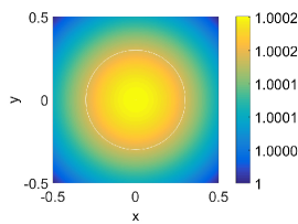
(a)

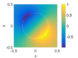
(b)

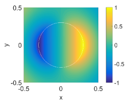
(c)

Figure 4: Representative modes near the origins of the LABEL:sub@fig:modecomparisonGXM1 $\Gamma$, LABEL:sub@fig:modecomparisonGXM2 $M$, and LABEL:sub@fig:modecomparisonGXM3 $X$ emanating band surfaces (for $\varepsilon_{\mathrm{c}}=1$ and $\mu_{\mathrm{c}}=2$, $\varepsilon_{\mathrm{c}}=-1$ and $\mu_{\mathrm{c}}=2$, and $\varepsilon_{\mathrm{c}}\approx-0.53$ and $\mu_{\mathrm{c}}\approx-10.22$ embedded in air, respectively). In all instances, the normalised $\mathrm{Re}(H_{\mathrm{z}})$ component of the field is given for lattice period $a=1$, cylinder radius $a^{\prime}=0.3a$ (boundary marked in white), and $L=1$.

For reference, in Fig. 4 we demonstrate the shape of the modes in the vicinity of their emanation points. In Fig. 4a we present the mode for $\varepsilon_{\mathrm{c}}=1$ and $\mu_{\mathrm{c}}=2$ in air with $\mathbf{k}_{\mathrm{B}}\approx(0,0)$ which shows that the mode is approximately constant as $\omega_{\mathrm{B}}\rightarrow 0$. This behaviour is typical for a crystal with such a low material contrast Bensoussan et al. (1978); Jikov et al. (1994). In Fig. 4b, we have $\varepsilon_{\mathrm{c}}=-1$ and $\mu_{\mathrm{c}}=2$ in air with $\mathbf{k}_{\mathrm{B}}\approx(\pi/a,\pi/a)$ which shows that the mode takes the form of a line dipole largely concentrated to the boundary of the cylinder. The dipole response is also oriented along $\theta=3\pi/4$ to ensure that the Bloch conditions are met along all edges of the unit cell (i.e., anti-periodicity). Finally, in Fig. 4c we give the mode for $\varepsilon_{\mathrm{c}}\approx-0.53$ and $\mu_{\mathrm{c}}\approx-10.22$ in air with $\mathbf{k}_{\mathrm{B}}\approx(\pi/a,0)$ which also shows a dipole response concentrated to the boundary of the cylinder. This dipole response is oriented along $\theta=\pi/2$ which ensures that the Bloch conditions are satisfied.

In Fig. 5 we present band diagrams for a crystal satisfying the conditions for $\Gamma$, $M$, and $X$ point emanation (given by (33), (42a) and (42b), and (46) and (49), respectively), but with a higher truncation value $L=5$. In all instances, the dashed red line represents the dipolar estimate of the first band surface. In Fig. 5a we observe that there are negligible differences between the few first band surfaces of a conventional photonic crystal, upon comparing Fig. 5a ($L=5$) with Fig. 1a of the letter ($L=1$). In Fig. 5b, we impose the $M$-point conditions for $L=1$ and evaluate the dispersion equation for $L=5$, and see that the conditions correctly predict the material parameters for which $M$ emanation occurs, but that the asymptotics are unable to correctly predict the slope. The higher bands are also different, but this is not unexpected as higher order multipole terms are generally required to reproduce both the dispersion relation and the modal fields at higher frequencies. We emphasize that this sensitivity is observed close to the $M$ point conditions alone (and is not observed away from $\varepsilon_{\mathrm{c}}=-\varepsilon_{\mathrm{b}}$), due to its correspondence with the anomalous resonance condition Bergman (1979); McPhedran and McKenzie (1980). We discuss this in further detail below. In Fig. 5c we impose the $X$-point conditions corresponding to $L=1$ for $L=5$, where we observe that the first two bands are well-approximated, but that the origin of the first band moves slightly away from $X$. Note that the first band is re-centred about $X$ after slightly perturbing the values of $\varepsilon_{\mathrm{c}}$ and $\mu_{\mathrm{c}}$. These variations in the band diagrams emphasise that the conditions and descriptions we obtain for $\Gamma$ and $X$ point emanation are good approximations for the full systems, but that our description of the first band emerging from $M$ are specific to the dipolar dispersion equation and are not necessarily accurate for higher truncations. Analytically determining high-truncation conditions poses a significant challenge, as the dispersion equation becomes highly intractable for large $L$.

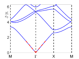
(a)

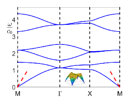
(b)

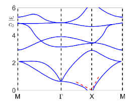
(c)

Figure 5: Band diagrams for square array of cylinders embedded in air ($\varepsilon_{\mathrm{b}}=\mu_{\mathrm{b}}=1$) with material properties LABEL:sub@fig:comparebands1 $\varepsilon_{\mathrm{c}}=1$ and $\mu_{\mathrm{c}}=2$, LABEL:sub@fig:comparebands2 $\varepsilon_{\mathrm{c}}=-1$ and $\mu_{\mathrm{c}}=2$ (inset: first band surface over first Brillouin zone), and LABEL:sub@fig:comparebands3 $\varepsilon_{\mathrm{c}}\approx-0.53$ and $\mu_{\mathrm{c}}\approx-10.22$. All figures use lattice period $a=1$, radius $a^{\prime}=0.3a$, and truncation $L=5$. Dashed red lines represent the dipolar first-band descriptions (32), (41), and (50b), respectively.

Returning to the discussion of anomalous resonances, these may be understood by analogy to (57); the zeros of $N_{l}$ and $N_{m}$ correspond to poles in the system at the angular orders $l$ and $m$, which at low frequencies, accumulate about $\varepsilon_{\mathrm{c}}=-\varepsilon_{\mathrm{b}}$ with increasing truncation $L$ (hence why anomalous resonances are also known as accumulation points). As such, in the vicinity of $\varepsilon_{\mathrm{c}}=-\varepsilon_{\mathrm{b}}$, the band diagrams for $L=1$ do not necessarily reflect the band diagrams for the full system, and we have found that results using other numerical tools, such as plane-wave expansion methods Busch and John (1998) and finite-element methods, exhibit extremely strong numerical instability with variations in the number of plane waves and the maximum element size, respectively. Preliminary results suggest that as we increase the truncation parameter $L\rightarrow\infty$, the slope of the first band tends to $\alpha^{\prime}\rightarrow 0$. We also find that the first band is only present at truncation values $L=1,2,5,6,9,10,\ldots$ (OEIS A042963) otherwise a low-frequency gap is observed; it is possible that the truncation order is tied to the existence of the first band (i.e., the truncation must be chosen to ensure that the system possesses the correct symmetries). This was observed earlier, where $M$ point emanation was not supported within a monopolar truncation. We remark that the issues observed with the $M$ point are not overcome through the use of other solution procedures, such as finite-element method (FEM) solvers (i.e., Comsol).

In fact, conventional FEM solvers are unable to validate the bands in Fig. 1 (Letter) centered about $M$ or $X$ at low frequencies. For the $M$ point, this is because the band diagrams returned by FEM solvers exhibit strong instability near the anomalous resonance condition. For the $X$ point, most commercially available solvers cannot evaluate bands when both the permittivity and permeability are negative-valued. However, it is possible to examine all band diagrams in Fig. 3 (Letter) using FEM solvers, excluding Figs. 3c and 3d, which cannot be validated due to their closeness to the anomalous resonance condition. We find that the conditions we derive herein give an excellent approximation to those obtained using a full FEM solver approach (i.e., the condition for Fig. 3e (Letter) is $\varepsilon_{\mathrm{c}}\approx-1.9$ using FEM solvers and not $\varepsilon_{\mathrm{c}}\approx-1.896$). Overall, we find that the dipole approximation gives a good description of both the conditions and the first band(s) when compared to those obtained with FEM solvers. For reference, the anomalous resonance condition $\varepsilon_{\mathrm{c}}=-\varepsilon_{\mathrm{b}}$ is identical for square and hexagonal lattices of cylinders McPhedran and McKenzie (1980), and that no analogy was found for the hexagonal lattice under the $X$ point conditions for a square lattice.

Regarding the issue of loss, if we incorporate loss in the background material (i.e., consider complex $\varepsilon_{\mathrm{b}}$ and $\mu_{\mathrm{b}}$), and then use the vanishing-determinant conditions to calculate the optical properties of the cylinder (thus obtaining complex $\varepsilon_{\mathrm{c}}$ and $\mu_{\mathrm{c}}$), then the corresponding band diagram (under the complex $\omega$ and real $k$ representation) is robust to moderately large imaginary values. Satisfying only the real parts of the background or cylinder materials constants may cause a gap to emerge about a band origin at low frequencies. Determining materials which satisfy the vanishing determinant conditions for complex-valued constants may pose something of a challenge, however it should be possible to engineer values for the permittivity and permeability with metamaterials as the cylinder media, for example.

As a final comment, we remark that large condition numbers are intrinsic for our cylindrical-Mie theory method, i.e. the discretised version of (20) or (57), even for conventional photonic crystals. Such numerical ill-conditioning poses a challenge for accurately determining band structures (as a numerically singular matrix may return spurious band surfaces). For $L=1$, we find that condition numbers are not prohibitively large, but due to the large values taken by $N_{l}$ and $S_{l}^{\mathrm{Y}}$ as $L\rightarrow\infty$, that ill-conditioning may pose a significant challenge for larger truncations (and is not corrected by the use of (57) in place of (20)).

VI Asymptotic forms of lattice sums for a square array

The cylindrical-Mie solution for a two-dimensional lattice of cylinders embedded in a uniform background material with permittivity $\varepsilon_{\mathrm{b}}$ and permeability $\mu_{\mathrm{b}}$ features sums of the form Chin et al. (1994); McPhedran et al. (1996); Movchan et al. (2002)

$$S_{l}^{\mathrm{Y}}(\omega_{\mathrm{B}},\mathbf{k}_{\mathrm{B}};n_{\mathrm{b}})=\sideset{}{{}^{\prime}}{\sum}_{(m,n)\in\mathbb{Z}^{2}}Y_{l}(n_{\mathrm{b}}\omega_{\mathrm{B}}R_{p})\mathrm{e}^{\mathrm{i}l\phi_{p}}\mathrm{e}^{\mathrm{i}\mathbf{k}_{\mathrm{B}}\cdot\mathbf{R}_{p}},$$ (58)

where $Y_{l}(z)$ is a Bessel function of the second kind, $\omega_{\mathrm{B}}=\omega/c_{0}$ is the scaled angular frequency, $n_{\mathrm{b}}=\sqrt{\varepsilon_{\mathrm{b}}}\sqrt{\mu_{\mathrm{b}}}$, $\mathbf{k}_{\mathrm{B}}$ is the in-plane Bloch vector, $(R_{p},\phi_{p})$ represents polar coordinates for the real lattice generator $\mathbf{R}_{p}=(ma,na)$, for $m,n\in\mathbb{Z}$, and prime notation denotes summation over the entire lattice excluding $(m,n)=(0,0)$, where the summand is singular. Here, the subscript $p$ represents a double index ranging over all $m$ and $n$. The lattice sum above is conditionally convergent, however, numerous procedures exist for accelerating convergence Linton (2010). One of these methods is to consider the reciprocal-space representation of (58); this is readily obtained by comparing forms of the quasi-periodic Green’s function for the Helmholtz operator defined by

$$\left\{\Delta+(n_{\mathrm{b}}\omega_{\mathrm{B}})^{2}\right\}G(\mathbf{x},\mathbf{x}^{\prime})=-2\pi\sum_{p}\delta(\mathbf{x}-\mathbf{x}^{\prime}-\mathbf{R}_{p})\mathrm{e}^{\mathrm{i}\mathbf{k}_{\mathrm{B}}\cdot\mathbf{R}_{p}}.$$ (59)

The comparison procedure is outlined in Movchan et al. (2002) and gives the absolutely convergent representation

$$S_{l}^{\mathrm{Y}}(\omega_{\mathrm{B}},\mathbf{k}_{\mathrm{B}};n_{\mathrm{b}})J_{l}(n_{\mathrm{b}}\omega_{\mathrm{B}}\xi)=-Y_{0}(n_{\mathrm{b}}\omega_{\mathrm{B}}\xi)\delta_{l0}-\frac{4\mathrm{i}^{l}}{A}\sum_{h}\frac{J_{l}(Q_{h}\xi)\mathrm{e}^{\mathrm{i}l\Theta_{h}}}{Q_{h}^{2}-(n_{\mathrm{b}}\omega_{\mathrm{B}})^{2}},$$ (60)

where $A$ denotes the area of the fundamental unit cell, $(K_{h},\psi_{h})$ are polar coordinates for the reciprocal lattice generator $\mathbf{K}_{h}=2\pi(m/a,n/a)$ for $m,n\in\mathbb{Z}$, $(Q_{h},\Theta_{h})$ denote polar coordinates for $\mathbf{Q}_{h}=\mathbf{K}_{h}+\mathbf{k}_{\mathrm{B}}$, and $(\xi,\gamma)$ represent polar coordinates for $\boldsymbol{\xi}=\mathbf{x}-\mathbf{x}^{\prime}$ (where we remark that $\psi_{h}$ and $\gamma$ are unused in the above, but are defined for completeness). Here, the subscript $h$ is a double index ranging over all $m$ and $n$. Note that $\boldsymbol{\xi}$, whilst defined as the difference between the source and field coordinates for the purposes of evaluating the Green’s function $G(\mathbf{x},\mathbf{x}^{\prime})$, now represents an arbitrary vector of finite length in the unit cell, as the lattice sums $S_{l}^{\mathrm{Y}}$ in (58) are independent of spatial coordinates.

VI.1 Asymptotic representations of dynamic lattice sums $S_{l}^{\mathrm{Y}}$ near $\Gamma$

We now present a brief summary of the method for determining the asymptotic forms of $S_{l}^{\mathrm{Y}}$ in the low frequency and vanishing Bloch vector limit, following the approach outlined in Appendix A of McPhedran et al. (1996). This begins by isolating the $h=(0,0)$ term in (60), and applying Graf’s addition theorem (Abramowitz and Stegun, 1972, Eq. (9.1.79)) to the surviving summand, admitting

$$S_{l}^{\mathrm{Y}}(\omega_{\mathrm{B}},\mathbf{k}_{\mathrm{B}};n_{\mathrm{b}})=-\frac{Y_{0}(n_{\mathrm{b}}\omega_{\mathrm{B}}\xi)}{J_{0}(n_{\mathrm{b}}\omega_{\mathrm{B}}\xi)}\delta_{l0}-\frac{4\mathrm{i}^{l}}{A}\frac{J_{l}(k_{\mathrm{B}}\xi)}{J_{l}(n_{\mathrm{b}}\omega_{\mathrm{B}}\xi)}\frac{\mathrm{e}^{\mathrm{i}l\theta_{\mathrm{B}}}}{k_{\mathrm{B}}^{2}-(n_{\mathrm{b}}\omega_{\mathrm{B}})^{2}}\\ -\frac{4\mathrm{i}^{l}}{A}\frac{1}{J_{l}(n_{\mathrm{b}}\omega_{\mathrm{B}}\xi)}\sideset{}{{}^{\prime}}{\sum}_{h}\sum_{m=-\infty}^{\infty}\frac{1}{Q_{h}^{2}-(n_{\mathrm{b}}\omega_{\mathrm{B}})^{2}}\left\{(-1)^{m}J_{l+m}(K_{h}\xi)J_{m}(k_{\mathrm{B}}\xi)\mathrm{e}^{\mathrm{i}(l+m)\psi_{h}-\mathrm{i}m\theta_{\mathrm{B}}}\right\},$$ (61)

where $(k_{\mathrm{B}},\theta_{\mathrm{B}})$ denotes the polar representation of the Bloch vector $\mathbf{k}_{\mathrm{B}}$. A Taylor series expansion for small $\omega_{\mathrm{B}}$ and $k_{\mathrm{B}}$ gives

$$\lim_{k_{\mathrm{B}}\rightarrow 0}\lim_{\omega_{\mathrm{B}}\rightarrow 0}\frac{1}{Q_{h}^{2}-(n_{\mathrm{b}}\omega_{\mathrm{B}})^{2}}\approx\frac{1}{K_{h}^{2}}\left(1-\frac{2k_{\mathrm{B}}}{K_{h}}\cos(\psi_{h}-\theta_{\mathrm{B}})+\frac{2k_{\mathrm{B}}^{2}}{K_{h}^{2}}\cos(2\left\{\psi_{h}-\theta_{\mathrm{B}}\right\})+\frac{k_{\mathrm{B}}^{2}+(n_{\mathrm{b}}\omega_{\mathrm{B}})^{2}}{K_{h}^{2}}+\ldots\right),$$ (62)

which after an appropriate truncation of $m$ in (61), and considerable algebraic manipulation, admits the asymptotic representations

$$\lim_{k_{\mathrm{B}}\rightarrow 0}\lim_{\omega_{\mathrm{B}}\rightarrow 0}\left\{S_{0}^{Y}\right\} \approx-\frac{Y_{0}(n_{\mathrm{b}}\omega_{\mathrm{B}}\xi)}{J_{0}(n_{\mathrm{b}}\omega_{\mathrm{B}}\xi)}-\frac{4}{A}\left\{\left(\frac{1}{k_{\mathrm{B}}^{2}-(n_{\mathrm{b}}\omega_{\mathrm{B}})^{2}}+S_{0,0,2}\right)\,\frac{J_{0}(k_{\mathrm{B}}\xi)}{J_{0}(n_{\mathrm{b}}\omega_{\mathrm{B}}\xi)}+2k_{\mathrm{B}}S_{1,0,3}\frac{J_{1}(k_{\mathrm{B}}\xi)}{J_{0}(n_{\mathrm{b}}\omega_{\mathrm{B}}\xi)}+\ldots\right\},$$ (63a)

$$\lim_{k_{\mathrm{B}}\rightarrow 0}\lim_{\omega_{\mathrm{B}}\rightarrow 0}\left\{S_{1}^{Y}\right\} \approx-\frac{4\mathrm{i}\mathrm{e}^{\mathrm{i}\theta_{\mathrm{B}}}}{A}\left\{\left(\frac{1}{k_{\mathrm{B}}^{2}-(n_{\mathrm{b}}\omega_{\mathrm{B}})^{2}}+S_{0,0,2}\right)\,\frac{J_{1}(k_{\mathrm{B}}\xi)}{J_{1}(n_{\mathrm{b}}\omega_{\mathrm{B}}\xi)}-k_{\mathrm{B}}S_{1,0,3}\frac{J_{0}(k_{\mathrm{B}}\xi)}{J_{1}(n_{\mathrm{b}}\omega_{\mathrm{B}}\xi)}+\ldots\right\},$$ (63b)

$$\lim_{k_{\mathrm{B}}\rightarrow 0}\lim_{\omega_{\mathrm{B}}\rightarrow 0}\left\{S_{2}^{Y}\right\} \approx\frac{4\mathrm{e}^{2\mathrm{i}\theta_{\mathrm{B}}}}{A}\left\{\left(\frac{1}{k_{\mathrm{B}}^{2}-(n_{\mathrm{b}}\omega_{\mathrm{B}})^{2}}+S_{0,0,2}\right)\frac{J_{2}(k_{\mathrm{B}}\xi)}{J_{2}(n_{\mathrm{b}}\omega_{\mathrm{B}}\xi)}-k_{\mathrm{B}}\,S_{1,0,3}\frac{J_{1}(k_{\mathrm{B}}\xi)}{J_{2}(n_{\mathrm{b}}\omega_{\mathrm{B}}\xi)}+k_{\mathrm{B}}^{\prime 2}\,S_{2,0,4}\frac{J_{0}(k_{\mathrm{B}}\xi)}{J_{2}(n_{\mathrm{b}}\omega_{\mathrm{B}}\xi)}\right\}$$

$$\qquad+\frac{4\mathrm{e}^{-2\mathrm{i}\theta_{\mathrm{B}}}}{A}\left\{S_{4,4,2}\,\frac{J_{2}(k_{\mathrm{B}}\xi)}{J_{2}(n_{\mathrm{b}}\omega_{\mathrm{B}}\xi)}+k_{\mathrm{B}}\,S_{3,4,3}\,\frac{J_{1}(k_{\mathrm{B}}\xi)}{J_{2}(n_{\mathrm{b}}\omega_{\mathrm{B}}\xi)}+k_{\mathrm{B}}^{2}\,S_{2,4,4}\,\frac{J_{0}(k_{\mathrm{B}}\xi)}{J_{2}(n_{\mathrm{b}}\omega_{\mathrm{B}}\xi)}+\ldots\right\},$$ (63c)

where we define the double Schömilch series Chen et al. (2018)

$$S_{l,m,n}(\xi;\tau,a)=\sum_{h}{}^{\prime}\frac{J_{l}(K_{h}\xi)}{K_{h}^{n}}\mathrm{e}^{\mathrm{i}m\psi_{h}}.$$ (64)

Using the explicit representations for $S_{l,m,n}$ in Chen et al. (2018), or the recurrence relation procedure in Nicorovici et al. (1996); McPhedran et al. (1996); Chen et al. (2018), we obtain

$$S_{0,0,2} =-\frac{a^{2}}{2\pi}\log(\xi)+\frac{a^{2}}{4\pi}\log\left(\frac{4\pi a^{2}}{\Gamma(\tfrac{1}{4})^{4}}\right)+\frac{\xi^{2}}{4},\quad S_{2,4,4}=\frac{a^{2}\xi^{2}\Gamma(\tfrac{1}{4})^{8}}{3\pi^{5}2^{12}}-\frac{\xi^{4}\Gamma(\tfrac{1}{4})^{8}}{9\pi^{4}2^{11}}+\frac{\xi^{6}\Gamma(\tfrac{1}{4})^{8}}{15\pi^{3}a^{2}2^{13}},$$ (65a)

$$S_{1,0,3} =-\frac{a^{2}\xi}{4\pi}\log(\xi)+\frac{a^{2}\xi}{8\pi}\log\left(\frac{4\pi a^{2}}{\Gamma(\tfrac{1}{4})^{4}}\right)+\frac{a^{2}\xi}{8\pi}+\frac{\xi^{3}}{16},\quad S_{3,4,3}=\frac{\xi^{3}\Gamma(\tfrac{1}{4})^{8}}{9\pi^{4}2^{10}}-\frac{\xi^{5}\Gamma(\tfrac{1}{4})^{8}}{15\pi^{3}a^{2}2^{11}},$$ (65b)

$$S_{2,0,4} =-\frac{a^{2}\xi^{2}}{16\pi}\log\left(\xi\right)+\frac{a^{2}\xi^{2}}{8\pi}\log\left(\frac{4\pi a^{2}}{\Gamma(\tfrac{1}{4})^{4}}\right)+\frac{3a^{2}\xi^{2}}{64\pi}+\frac{\xi^{4}}{96},\quad S_{4,4,2}=\frac{\xi^{4}\Gamma(\tfrac{1}{4})^{8}}{15\pi^{3}a^{2}2^{10}},$$ (65c)

for a square lattice of period $a$. The $S_{l,m,n}$ expressions above in tandem with the small argument expansions McPhedran et al. (1996)

$$\lim_{\xi\rightarrow 0}\lim_{k_{\mathrm{B}}\rightarrow 0}\lim_{\omega_{\mathrm{B}}\rightarrow 0}\frac{Y_{0}(n_{\mathrm{b}}\omega_{\mathrm{B}}\xi)}{J_{0}(n_{\mathrm{b}}\omega_{\mathrm{B}}\xi)} \approx\frac{2}{\pi}\left(\gamma_{\mathrm{e}}+\log\left(\frac{n_{\mathrm{b}}\omega_{\mathrm{B}}\xi}{2}\right)\right)+\frac{(n_{\mathrm{b}}\omega_{\mathrm{B}})^{2}\xi^{2}}{2\pi}+\ldots,$$ (66a)

$$\lim_{\xi\rightarrow 0}\lim_{k_{\mathrm{B}}\rightarrow 0}\lim_{\omega_{\mathrm{B}}\rightarrow 0}\frac{J_{0}(k_{\mathrm{B}}\xi)}{J_{0}(n_{\mathrm{b}}\omega_{\mathrm{B}}\xi)} \approx 1+\frac{(n_{\mathrm{b}}\omega_{\mathrm{B}})^{2}-k_{\mathrm{B}}^{2}}{4}\xi^{2}+\ldots,$$ (66b)

$$\lim_{\xi\rightarrow 0}\lim_{k_{\mathrm{B}}\rightarrow 0}\lim_{\omega_{\mathrm{B}}\rightarrow 0}\frac{J_{1}(k_{\mathrm{B}}\xi)}{J_{1}(n_{\mathrm{b}}\omega_{\mathrm{B}}\xi)} \approx\frac{k_{\mathrm{B}}}{n_{\mathrm{b}}\omega_{\mathrm{B}}}+\frac{k_{\mathrm{B}}}{n_{\mathrm{b}}\omega_{\mathrm{B}}}\frac{(n_{\mathrm{b}}\omega_{\mathrm{B}})^{2}-k_{\mathrm{B}}^{2}}{8}\xi^{2}+\ldots,$$ (66c)

$$\lim_{\xi\rightarrow 0}\lim_{k_{\mathrm{B}}\rightarrow 0}\lim_{\omega_{\mathrm{B}}\rightarrow 0}\frac{J_{0}(k_{\mathrm{B}}\xi)}{J_{1}(n_{\mathrm{b}}\omega_{\mathrm{B}}\xi)} \approx\frac{2}{n_{\mathrm{b}}\omega_{\mathrm{B}}\xi}+\frac{(n_{\mathrm{b}}\omega_{\mathrm{B}})^{2}-2k_{\mathrm{B}}^{2}}{4n_{\mathrm{b}}\omega_{\mathrm{B}}}\xi+\left(\frac{1}{32}\frac{k_{\mathrm{B}}}{n_{\mathrm{b}}\omega_{\mathrm{B}}}-\frac{1}{16}\frac{n_{\mathrm{b}}\omega_{\mathrm{B}}}{k_{\mathrm{B}}}+\frac{1}{48}\frac{(n_{\mathrm{b}}\omega_{\mathrm{B}})^{3}}{k_{\mathrm{B}}^{3}}\right)k_{\mathrm{B}}^{3}\xi^{3}+\ldots,$$ (66d)

$$\lim_{\xi\rightarrow 0}\lim_{k_{\mathrm{B}}\rightarrow 0}\lim_{\omega_{\mathrm{B}}\rightarrow 0}\frac{J_{1}(k_{\mathrm{B}}\xi)}{J_{0}(n_{\mathrm{b}}\omega_{\mathrm{B}}\xi)} \approx\frac{k_{\mathrm{B}}\xi}{2}+\frac{2(n_{\mathrm{b}}\omega_{\mathrm{B}})^{2}-k_{\mathrm{B}}^{2}}{16}k_{\mathrm{B}}\xi^{3}+\ldots,$$ (66e)

$$\lim_{\xi\rightarrow 0}\lim_{k_{\mathrm{B}}\rightarrow 0}\lim_{\omega_{\mathrm{B}}\rightarrow 0}\frac{J_{0}(k_{\mathrm{B}}\xi)}{J_{2}(n_{\mathrm{b}}\omega_{\mathrm{B}}\xi)} \approx\frac{8}{(n_{\mathrm{b}}\omega_{\mathrm{B}})^{2}\xi^{2}}+2\left(\frac{1}{3}-\frac{k_{\mathrm{B}}^{2}}{(n_{\mathrm{b}}\omega_{\mathrm{B}})^{2}}\right)+\left(-\frac{1}{6}+\frac{1}{8}\frac{k_{\mathrm{B}}^{2}}{(n_{\mathrm{b}}\omega_{\mathrm{B}})^{2}}+\frac{5}{144}\frac{(n_{\mathrm{b}}\omega_{\mathrm{B}})^{2}}{k_{\mathrm{B}}^{2}}\right)k_{\mathrm{B}}^{2}\xi^{2}+\ldots,$$ (66f)

$$\lim_{\xi\rightarrow 0}\lim_{k_{\mathrm{B}}\rightarrow 0}\lim_{\omega_{\mathrm{B}}\rightarrow 0}\frac{J_{1}(k_{\mathrm{B}}\xi)}{J_{2}(n_{\mathrm{b}}\omega_{\mathrm{B}}\xi)} \approx\frac{4k_{\mathrm{B}}}{(n_{\mathrm{b}}\omega_{\mathrm{B}})^{2}\xi}+\frac{2(n_{\mathrm{b}}\omega_{\mathrm{B}})^{2}-3k_{\mathrm{B}}^{2}}{6(n_{\mathrm{b}}\omega_{\mathrm{B}})^{2}}k_{\mathrm{B}}\xi+\left(-\frac{1}{24}+\frac{1}{48}\frac{k_{\mathrm{B}}^{2}}{(n_{\mathrm{b}}\omega_{\mathrm{B}})^{2}}+\frac{5}{288}\frac{(n_{\mathrm{b}}\omega_{\mathrm{B}})^{2}}{k_{\mathrm{B}}^{2}}\right)k_{\mathrm{B}}^{3}\xi^{3}+\ldots,$$ (66g)

$$\lim_{\xi\rightarrow 0}\lim_{k_{\mathrm{B}}\rightarrow 0}\lim_{\omega_{\mathrm{B}}\rightarrow 0}\frac{J_{2}(k_{\mathrm{B}}\xi)}{J_{2}(n_{\mathrm{b}}\omega_{\mathrm{B}}\xi)} \approx\frac{k_{\mathrm{B}}^{2}}{(n_{\mathrm{b}}\omega_{\mathrm{B}})^{2}}+\frac{k_{\mathrm{B}}^{2}}{(n_{\mathrm{b}}\omega_{\mathrm{B}})^{2}}\frac{(n_{\mathrm{b}}\omega_{\mathrm{B}})^{2}-k_{\mathrm{B}}^{2}}{12}\xi^{2}+\ldots,$$ (66h)

finally admit the representations (26) for $S_{0}^{\mathrm{Y}}$, $S_{1}^{\mathrm{Y}}$, and $S_{2}^{\mathrm{Y}}$ both at low frequencies and in the vicinity of the $\Gamma$ point, after extensive algebraic manipulation.

VI.2 Asymptotic representations of dynamic lattice sums $S_{l}^{\mathrm{Y}}$ near $M$

To obtain closed-form representations for $S_{l}^{\mathrm{Y}}$ in the vicinity of different symmetry points (and also for vanishing $\omega_{\mathrm{B}}$) we extend the procedure above. The approach is identical up to (61), however, to consider behaviour near the $M$ point it is necessary to modify (62) appropriately. This is achieved by decomposing the translated reciprocal lattice generator as $\mathbf{Q}_{h}=\mathbf{K}_{h}+\mathbf{k}_{\mathrm{B}}=(\mathbf{K}_{h}+\mathbf{M})+(\mathbf{k}_{\mathrm{B}}-\mathbf{M})=\mathbf{K}_{h}^{\prime}+\mathbf{k}_{\mathrm{B}}^{\prime}$, where $\mathbf{M}=(\pi/a,\pi/a)$. Substituting this decomposition into (62), we recover an identical expression to before, but with the replacements $\mathbf{K}_{h}\mapsto\mathbf{K}_{h}^{\prime}$ and $\mathbf{k}_{\mathrm{B}}\mapsto\mathbf{k}_{\mathrm{B}}^{\prime}$ and an updated limit argument. Subsequently we obtain analogous expressions to (63) but without the singular terms $1/(k_{\mathrm{B}}^{2}-(n_{\mathrm{b}}\omega_{\mathrm{B}})^{2})$, as light lines are not present near $M$ at low frequencies. That is, for the $M$ point we obtain

$$\lim_{k_{\mathrm{B}}\rightarrow M}\lim_{\omega_{\mathrm{B}}\rightarrow 0}\left\{S_{0}^{Y}\right\} \approx-\frac{Y_{0}(n_{\mathrm{b}}\omega_{\mathrm{B}}\xi)}{J_{0}(n_{\mathrm{b}}\omega_{\mathrm{B}}\xi)}-\frac{4}{A}\left\{S_{0,0,2}^{\mathrm{M}}\,\frac{J_{0}(k_{\mathrm{B}}^{\prime}\xi)}{J_{0}(n_{\mathrm{b}}\omega_{\mathrm{B}}\xi)}+2k_{\mathrm{B}}^{\prime}S_{1,0,3}^{\mathrm{M}}\frac{J_{1}(k_{\mathrm{B}}^{\prime}\xi)}{J_{0}(n_{\mathrm{b}}\omega_{\mathrm{B}}\xi)}\right\},$$ (67a)

$$\lim_{k_{\mathrm{B}}\rightarrow M}\lim_{\omega_{\mathrm{B}}\rightarrow 0}\left\{S_{1}^{Y}\right\} \approx-\frac{4\mathrm{i}\mathrm{e}^{\mathrm{i}\theta_{\mathrm{B}}^{\prime}}}{A}\left\{S_{0,0,2}^{\mathrm{M}}\,\frac{J_{1}(k_{\mathrm{B}}^{\prime}\xi)}{J_{1}(n_{\mathrm{b}}\omega_{\mathrm{B}}\xi)}-k_{\mathrm{B}}^{\prime}S_{1,0,3}^{\mathrm{M}}\frac{J_{0}(k_{\mathrm{B}}^{\prime}\xi)}{J_{1}(n_{\mathrm{b}}\omega_{\mathrm{B}}\xi)}\right\},$$ (67b)

$$\lim_{k_{\mathrm{B}}\rightarrow M}\lim_{\omega_{\mathrm{B}}\rightarrow 0}\left\{S_{2}^{Y}\right\} \approx\frac{4\mathrm{e}^{2\mathrm{i}\theta_{\mathrm{B}}^{\prime}}}{A}\left\{S_{0,0,2}^{\mathrm{M}}\frac{J_{2}(k_{\mathrm{B}}^{\prime}\xi)}{J_{2}(n_{\mathrm{b}}\omega_{\mathrm{B}}\xi)}-k_{\mathrm{B}}^{\prime}\,S_{1,0,3}^{\mathrm{M}}\frac{J_{1}(k_{\mathrm{B}}^{\prime}\xi)}{J_{2}(n_{\mathrm{b}}\omega_{\mathrm{B}}\xi)}+k_{\mathrm{B}}^{\prime 2}\,S_{2,0,4}^{\mathrm{M}}\frac{J_{0}(k_{\mathrm{B}}^{\prime}\xi)}{J_{2}(n_{\mathrm{b}}\omega_{\mathrm{B}}\xi)}\right\}$$

$$\qquad+\frac{4\mathrm{e}^{-2\mathrm{i}\theta_{\mathrm{B}}^{\prime}}}{A}\left\{S_{4,4,2}^{\mathrm{M}}\,\frac{J_{2}(k_{\mathrm{B}}^{\prime}\xi)}{J_{2}(n_{\mathrm{b}}\omega_{\mathrm{B}}\xi)}+k_{\mathrm{B}}^{\prime}\,S_{3,4,3}^{\mathrm{M}}\,\frac{J_{1}(k_{\mathrm{B}}^{\prime}\xi)}{J_{2}(n_{\mathrm{b}}\omega_{\mathrm{B}}\xi)}+k_{\mathrm{B}}^{\prime 2}\,S_{2,4,4}^{\mathrm{M}}\,\frac{J_{0}(k_{\mathrm{B}}^{\prime}\xi)}{J_{2}(n_{\mathrm{b}}\omega_{\mathrm{B}}\xi)}\right\},$$ (67c)

where we emphasise that $\boldsymbol{\xi}$ is an arbitrary vector in the first Brillouin zone that remains untranslated, $(k_{\mathrm{B}}^{\prime},\theta_{\mathrm{B}}^{\prime})$ is the polar representation of $\mathbf{k}_{\mathrm{B}}^{\prime}=\mathbf{k}_{\mathrm{B}}-\mathbf{M}$, and

$$S_{l,m,n}^{\mathrm{M}}(\xi;\tau,a)=\sum_{h}{}^{\prime}\frac{J_{l}(K_{h}^{\prime}\xi)}{K_{h}^{\prime n}}\mathrm{e}^{\mathrm{i}m\psi_{h}^{\prime}},$$ (68)

where $(K_{h}^{\prime},\psi_{h}^{\prime})$ is the polar representation of $\mathbf{K}_{h}^{\prime}=\mathbf{K}_{h}+\mathbf{M}$. As highlighted in Chen et al. (2018), analytical expressions for $S_{l,m,n}^{\mathrm{M}}$, corresponding to Bloch vectors centred around the $M$ point, are easily obtained by evaluating a selection of rectangular and square $\Gamma$-centred sums and using the multi-set identity Chen et al. (2018)

$$\mkern 1.5mu\overline{\mkern-1.5mu\Omega\mkern-1.5mu}\mkern 1.5mu^{M}(\mathrm{i},a)=\mkern 1.5mu\overline{\mkern-1.5mu\Omega\mkern-1.5mu}\mkern 1.5mu(\mathrm{i},2a)-\mkern 1.5mu\overline{\mkern-1.5mu\Omega\mkern-1.5mu}\mkern 1.5mu(\mathrm{i}/2,2a)+\mkern 1.5mu\overline{\mkern-1.5mu\Omega\mkern-1.5mu}\mkern 1.5mu(\mathrm{i},a)-\mkern 1.5mu\overline{\mkern-1.5mu\Omega\mkern-1.5mu}\mkern 1.5mu(2\mathrm{i},a),$$ (69a)

where $$\mkern 1.5mu\overline{\mkern-1.5mu\Omega\mkern-1.5mu}\mkern 1.5mu$$ are reciprocal lattice sets defined by

$$\mkern 1.5mu\overline{\mkern-1.5mu\Omega\mkern-1.5mu}\mkern 1.5mu(\tau,a)=\left\{\frac{2\pi}{A}(h_{1}b\hat{\mathbf{e}}_{1}^{\prime}+h_{2}a\hat{\mathbf{e}}_{2}^{\prime})\bigg{|}h_{1},h_{2}\in\mathbb{Z}\right\},$$ (69b)

with $A=ab$ representing the area of the unit cell (for a rectangular lattice of periods $a$ and $b$ in $x$ and $y$ respectively), $\hat{\mathbf{e}}_{j}^{\prime}$ are basis vectors for the reciprocal lattice, and $\tau=(b/a)\mathrm{i}$. The multi-set identity (69a) gives the following expressions

$$S_{0,0,2}^{\mathrm{M}} =-\frac{a^{2}}{2\pi}\log\left(\xi\right)+\frac{a^{2}}{4\pi}\log\left(\frac{16\pi a^{2}}{\Gamma(\tfrac{1}{4})^{4}}\right),\quad S_{2,4,4}^{\mathrm{M}}=-\frac{\xi^{6}\Gamma(\tfrac{1}{4})^{8}}{5\pi^{3}a^{2}2^{14}}+\frac{\xi^{4}\Gamma(\tfrac{1}{4})^{8}}{9\pi^{4}2^{10}}-\frac{a^{2}\xi^{2}\Gamma(\tfrac{1}{4})^{8}}{\pi^{5}2^{12}},$$ (70a)

$$S_{1,0,3}^{\mathrm{M}} =\frac{a^{2}\xi}{8\pi}-\frac{a^{2}\xi}{4\pi}\log\left(\xi\right)+\frac{a^{2}\xi}{8\pi}\log\left(\frac{16\pi a^{2}}{\Gamma(\tfrac{1}{4})^{4}}\right),\quad S_{3,4,3}^{\mathrm{M}}=\frac{\xi^{5}\Gamma(\tfrac{1}{4})^{8}}{5\pi^{3}a^{2}2^{12}}-\frac{\xi^{3}\Gamma(\tfrac{1}{4})^{8}}{9\pi^{4}2^{9}},$$ (70b)

$$S_{2,0,4}^{\mathrm{M}} =\frac{3a^{2}\xi^{2}}{64\pi}-\frac{a^{2}\xi^{2}}{16\pi}\log\left(\xi\right)+\frac{a^{2}\xi^{2}}{32\pi}\log\left(\frac{16\pi a^{2}}{\Gamma(\tfrac{1}{4})^{4}}\right),\quad S_{4,4,2}^{\mathrm{M}}=-\frac{\xi^{4}\Gamma(\tfrac{1}{4})^{8}}{5\pi^{3}a^{2}2^{11}}.$$ (70c)

Substituting the $S_{l,m,n}^{\mathrm{M}}$ expressions (70) and the Bessel function expansions (66) into the expansions for $S_{l}^{\mathrm{Y}}$ (67) above ultimately gives the final expressions (35) used in Section III.2.

VI.3 Asymptotic representations of $S_{l}^{\mathrm{Y}}$ at the $X$ point

As with the $M$ point approach, in order to consider behaviour near the $X$ point it is necessary to modify (62) appropriately. Decomposing $\mathbf{Q}_{h}=\mathbf{K}_{h}+\mathbf{k}_{\mathrm{B}}=(\mathbf{K}_{h}+\mathbf{X})+(\mathbf{k}_{\mathrm{B}}-\mathbf{X})$, where $\mathbf{X}=(\pi/a,0)$ into (62) we obtain

$$\lim_{k_{\mathrm{B}}\rightarrow X}\lim_{\omega_{\mathrm{B}}\rightarrow 0}S_{0}^{\mathrm{Y}}\approx-\frac{Y_{0}(n_{\mathrm{b}}\omega_{\mathrm{B}}\xi)}{J_{0}(n_{\mathrm{b}}\omega_{\mathrm{B}}\xi)}-\frac{4}{A}\frac{J_{0}(k_{\mathrm{B}}^{\prime\prime}\xi)}{J_{0}(n_{\mathrm{b}}\omega_{\mathrm{B}}\xi)}\left(S_{0,0,2}^{\mathrm{X}}+(n_{\mathrm{b}}\omega_{\mathrm{B}})^{2}S_{0,0,4}^{\mathrm{X}}+k_{\mathrm{B}}^{{\prime\prime}2}S_{0,0,4}^{\mathrm{X}}\right)\\ -\frac{4}{A}\frac{J_{0}(k_{\mathrm{B}}^{\prime\prime}\xi)}{J_{0}(n_{\mathrm{b}}\omega_{\mathrm{B}}\xi)}\mathrm{e}^{-2\mathrm{i}\theta_{\mathrm{B}}^{\prime\prime}}\left(k_{\mathrm{B}}^{{\prime\prime}2}S_{0,2,4}^{\mathrm{X}}\right)-\frac{4}{A}\frac{J_{0}(k_{\mathrm{B}}^{\prime\prime}\xi)}{J_{0}(n_{\mathrm{b}}\omega_{\mathrm{B}}\xi)}\mathrm{e}^{2\mathrm{i}\theta_{\mathrm{B}}^{\prime\prime}}\left(k_{\mathrm{B}}^{{\prime\prime}2}S_{0,2,4}^{\mathrm{X}}\right),$$ (71a)

$$\lim_{k_{\mathrm{B}}\rightarrow X}\lim_{\omega_{\mathrm{B}}\rightarrow 0}S_{1}^{\mathrm{Y}}\approx-\frac{4\mathrm{i}\mathrm{e}^{\mathrm{i}\theta_{\mathrm{B}}^{\prime\prime}}}{A}\frac{J_{1}(k_{\mathrm{B}}^{\prime\prime}\xi)}{J_{1}(n_{\mathrm{b}}\omega_{\mathrm{B}}\xi)}\left(S_{0,0,2}^{\mathrm{X}}+(n_{\mathrm{b}}\omega_{\mathrm{B}})^{2}S_{0,0,4}^{\mathrm{X}}+k_{\mathrm{B}}^{{\prime\prime}2}S_{0,0,4}^{\mathrm{X}}\right)+\frac{4\mathrm{i}\mathrm{e}^{\mathrm{i}\theta_{\mathrm{B}}^{\prime\prime}}}{A}\frac{J_{0}(k_{\mathrm{B}}^{\prime\prime}\xi)}{J_{1}(n_{\mathrm{b}}\omega_{\mathrm{B}}\xi)}\left(k_{\mathrm{B}}^{{\prime\prime}}S_{1,0,3}^{\mathrm{X}}\right)\\ +\frac{4\mathrm{i}\mathrm{e}^{-\mathrm{i}\theta_{\mathrm{B}}^{\prime\prime}}}{A}\frac{J_{0}(k_{\mathrm{B}}^{\prime\prime}\xi)}{J_{1}(n_{\mathrm{b}}\omega_{\mathrm{B}}\xi)}\left(k_{\mathrm{B}}^{{\prime\prime}}S_{1,2,3}^{\mathrm{X}}\right)-\frac{4\mathrm{i}\mathrm{e}^{-\mathrm{i}\theta_{\mathrm{B}}^{\prime\prime}}}{A}\frac{J_{1}(k_{\mathrm{B}}^{\prime\prime}\xi)}{J_{1}(n_{\mathrm{b}}\omega_{\mathrm{B}}\xi)}\left(k_{\mathrm{B}}^{{\prime\prime}2}S_{0,2,4}^{\mathrm{X}}\right),$$ (71b)

$$\lim_{k_{\mathrm{B}}\rightarrow X}\lim_{\omega_{\mathrm{B}}\rightarrow 0}S_{2}^{\mathrm{Y}}\approx\frac{4}{A}\frac{J_{0}(k_{\mathrm{B}}^{\prime\prime}\xi)}{J_{2}(n_{\mathrm{b}}\omega_{\mathrm{B}}\xi)}\left(S_{2,2,2}^{\mathrm{X}}+(n_{\mathrm{b}}\omega_{\mathrm{B}})^{2}S_{2,2,4}^{\mathrm{X}}+k_{\mathrm{B}}^{{\prime\prime}2}S_{2,2,4}^{\mathrm{X}}\right)-\frac{4}{A}\frac{J_{1}(k_{\mathrm{B}}^{\prime\prime}\xi)}{J_{2}(n_{\mathrm{b}}\omega_{\mathrm{B}}\xi)}\left(k_{\mathrm{B}}^{\prime\prime}S_{1,2,3}^{\mathrm{X}}\right)\\ +\frac{4}{A}\frac{J_{2}(k_{\mathrm{B}}^{\prime\prime}\xi)}{J_{2}(n_{\mathrm{b}}\omega_{\mathrm{B}}\xi)}\left(k_{\mathrm{B}}^{{\prime\prime}2}S_{0,2,4}^{\mathrm{X}}\right)+\frac{4\mathrm{e}^{2\mathrm{i}\theta_{\mathrm{B}}^{\prime\prime}}}{A}\frac{J_{2}(k_{\mathrm{B}}^{\prime\prime}\xi)}{J_{2}(n_{\mathrm{b}}\omega_{\mathrm{B}}\xi)}\left(S_{0,0,2}^{\mathrm{X}}+(n_{\mathrm{b}}\omega_{\mathrm{B}})^{2}S_{0,0,4}^{\mathrm{X}}+k_{\mathrm{B}}^{{\prime\prime}2}S_{0,0,4}^{\mathrm{X}}\right)\\ +\frac{4\mathrm{e}^{2\mathrm{i}\theta_{\mathrm{B}}^{\prime\prime}}}{A}\frac{J_{1}(k_{\mathrm{B}}^{\prime\prime}\xi)}{J_{2}(n_{\mathrm{b}}\omega_{\mathrm{B}}\xi)}\left(-k_{\mathrm{B}}^{\prime\prime}S_{1,0,3}^{\mathrm{X}}\right)+\frac{4\mathrm{e}^{2\mathrm{i}\theta_{\mathrm{B}}^{\prime\prime}}}{A}\frac{J_{0}(k_{\mathrm{B}}^{\prime\prime}\xi)}{J_{2}(n_{\mathrm{b}}\omega_{\mathrm{B}}\xi)}\left(k_{\mathrm{B}}^{{\prime\prime}2}S_{2,0,4}^{\mathrm{X}}\right)+\frac{4\mathrm{e}^{-2\mathrm{i}\theta_{\mathrm{B}}^{\prime\prime}}}{A}\frac{J_{0}(k_{\mathrm{B}}^{\prime\prime}\xi)}{J_{2}(n_{\mathrm{b}}\omega_{\mathrm{B}}\xi)}\left(k_{\mathrm{B}}^{{\prime\prime}2}S_{2,4,4}^{\mathrm{X}}\right),$$ (71c)

where $\mathbf{k}_{\mathrm{B}}^{\prime\prime}=\mathbf{k}_{\mathrm{B}}-\mathbf{X}$ with polar representation $(k_{\mathrm{B}}^{\prime\prime},\theta_{\mathrm{B}}^{\prime\prime})$, $\mathbf{K}_{h}^{\prime\prime}=\mathbf{K}_{h}+\mathbf{X}$ with polar representation $(K_{h}^{\prime\prime},\psi_{h}^{\prime\prime})$, and

$$S_{l,m,n}^{\mathrm{X}}(\xi;\tau,a)=\sum_{h}{}^{\prime}\frac{J_{l}(K_{h}^{\prime\prime}\xi)}{K_{h}^{{\prime\prime}n}}\mathrm{e}^{\mathrm{i}m\psi_{h}^{\prime\prime}},$$ (72)

Note that in contrast to the representations for $S_{l}^{\mathrm{Y}}$ in (63) and (67), the closed-form representations for $S_{l}^{\mathrm{Y}}$ near the $X$ point have a considerably different structure. This is because only two-fold symmetry is possessed near the $X$ point at low frequencies. The $S_{l,m,n}^{\mathrm{X}}$ are evaluated using the multi-set identity Chen et al. (2018)

$$\mkern 1.5mu\overline{\mkern-1.5mu\Omega\mkern-1.5mu}\mkern 1.5mu^{X}(\mathrm{i},a)=\mkern 1.5mu\overline{\mkern-1.5mu\Omega\mkern-1.5mu}\mkern 1.5mu(\mathrm{i}/2,2a)-\mkern 1.5mu\overline{\mkern-1.5mu\Omega\mkern-1.5mu}\mkern 1.5mu(\mathrm{i},a),$$ (73)

to obtain

$$S_{0,0,2}^{\mathrm{X}} =-\frac{a^{2}}{2\pi}\log(\xi)+\frac{a^{2}}{4\pi}\log\left(\frac{32\pi a^{2}}{\Gamma(\tfrac{1}{4})^{4}}\right),\quad S_{0,0,4}^{\mathrm{X}}=\frac{3a^{4}}{2\pi^{4}}\zeta(2)\beta(2)-\frac{a^{2}\xi^{2}}{8\pi}+\frac{a^{2}\xi^{2}}{8\pi}\log(\xi)-\frac{a^{2}\xi^{2}}{16\pi}\log\left(\frac{32\pi a^{2}}{\Gamma(\tfrac{1}{4})^{4}}\right),$$ (74a)

$$S_{0,2,4}^{\mathrm{X}} =-\frac{a^{2}\Gamma(\tfrac{1}{4})^{4}}{128\pi^{3}}\xi^{2}+\frac{\Gamma(\tfrac{1}{4})^{4}}{1024\pi^{2}}\xi^{4}-\frac{a^{4}}{16\pi^{4}}G_{4}^{(2)}(\tfrac{\mathrm{i}}{2}),\quad S_{1,0,3}^{\mathrm{X}}=\frac{a^{2}\xi}{8\pi}-\frac{a^{2}\xi}{4\pi}\log(\xi)+\frac{a^{2}\xi}{8\pi}\log\left(\frac{32\pi a^{2}}{\Gamma(\tfrac{1}{4})^{4}}\right),$$ (74b)

$$S_{1,2,3}^{\mathrm{X}} =\frac{a^{2}\Gamma(\tfrac{1}{4})^{4}}{64\pi^{3}}\xi-\frac{\Gamma(\tfrac{1}{4})^{4}}{256\pi^{2}}\xi^{3},\quad S_{2,0,4}^{\mathrm{X}}=\frac{3a^{2}\xi^{2}}{64\pi}-\frac{a^{2}\xi^{2}}{16\pi}\log(\xi)+\frac{a^{2}\xi^{2}}{32\pi}\log\left(\frac{32\pi a^{2}}{\Gamma(\tfrac{1}{4})^{4}}\right),$$ (74c)

$$S_{2,2,2}^{\mathrm{X}} =\frac{\Gamma(\tfrac{1}{4})^{4}}{128\pi^{2}}\xi^{2},\quad S_{2,2,4}^{\mathrm{X}}=\frac{a^{2}\Gamma(\tfrac{1}{4})^{4}}{256\pi^{3}}\xi^{2}-\frac{\Gamma(\tfrac{1}{4})^{4}}{3\pi^{2}2^{9}}\xi^{4},\quad S_{2,4,4}^{\mathrm{X}}=\frac{\xi^{6}\Gamma(\tfrac{1}{4})^{8}}{5\pi^{3}a^{2}2^{16}}-\frac{\xi^{4}\Gamma(\tfrac{1}{4})^{8}}{9\pi^{4}2^{11}}+\frac{a^{2}\xi^{2}\Gamma(\tfrac{1}{4})^{8}}{\pi^{5}2^{12}},$$ (74d)

where $\zeta(s)$ denotes the Riemann zeta function and $\beta(s)$ the Dirichlet beta function. Note that closed form expressions are not generally available for phase-conjugated Eisenstein series $G_{n}^{(m)}$ when $m<n$ (for reference, $G_{4}^{(2)}(\tfrac{\mathrm{i}}{2})\approx-30.854212880849047$ and is given as a rapidly convergent sum in Chen et al. (2018)). Substituting (66) and (74) into the asymptotic approximations (71) above gives the final expressions (43) presented in Section III.3.

As a final comment, we remark that obtaining closed-form expressions for $S_{l}^{\mathrm{Y}}$ about other points in the Brillouin zone may pose something of a challenge as these do not have multiset representations using origin centered lattices. The $X$ and $M$ points are special cases where multiset representations are possible due to symmetry, despite not being origin centered lattices themselves.

References

• Joannopoulos et al. (2008) J. D. Joannopoulos, S. G. Johnson, J. N. Winn,  and R. D. Meade, Photonic Crystals: Molding the Flow of Light (Princeton University Press, Princeton, 2008).
• Born and Wolf (1964) M. Born and E. Wolf, Principles of Optics: Electromagnetic Theory of Propagation, Interference and Diffraction of Light (Pergamon Press, New York, 1964).
• Kittel (2005) C. Kittel, Introduction to Solid State Physics (John Wiley & Sons, New York, 2005).
• Smith et al. (2004) D. R. Smith, J. B. Pendry,  and M. C. K. Wiltshire, Science 305, 788 (2004).
• Veselago (1968) V. G. Veselago, Sov. Phys. Usp. 10, 509 (1968).
• Pendry (2000) J. B. Pendry, Phys. Rev. Lett. 85, 3966 (2000).
• Fan et al. (1996) S. Fan, P. R. Villeneuve,  and J. D. Joannopoulos, Phys. Rev. B 54, 11245 (1996).
• Lerario et al. (2017) G. Lerario, A. Fieramosca, F. Barachati, D. Ballarini, K. S. Daskalakis, L. Dominici, M. De Giorgi, S. A. Maier, G. Gigli, S. Kéna-Cohen, et al., Nat. Phys. 13, 837 (2017).
• Chen et al. (2011) P. Y. Chen, C. G. Poulton, A. A. Asatryan, M. J. Steel, L. C. Botten, C. M. de Sterke,  and R. C. McPhedran, New J. Phys. 13, 053007 (2011).
• Guenneau et al. (2007) S. Guenneau, S. Anatha Ramakrishna, S. Enoch, S. Chakrabarti, G. Tayeb,  and B. Gralak, Photonics Nanostruct. 5, 63 (2007).
• Helsing et al. (2011) J. Helsing, R. C. McPhedran,  and G. W. Milton, New J. Phys. 13, 115005 (2011).
• Li et al. (2003) J. Li, L. Zhou, C. T. Chan,  and P. Sheng, Phys. Rev. Lett. 90, 083901 (2003).
• Harrison (1989) W. A. Harrison, Electronic Structure and the Properties of Solids: the Physics of the Chemical Bond (Dover, New York, 1989).
• Cora et al. (1997) F. Cora, M. Stachiotti, C. Catlow,  and C. Rodriguez, J. Phys. Chem. B 101, 3945 (1997).
• Movchan et al. (2002) A. B. Movchan, N. V. Movchan,  and C. G. Poulton, Asymptotic Models of Fields in Dilute and Densely Packed Composites (Imperial College Press, London, 2002).
• (16) See Supplemental Material for definitions of lattice sums, derivations of asymptotic forms, and detailed discussions, which includes Refs. McPhedran et al. (1996); Poulton et al. (2000); McPhedran et al. (2000); Linton (1998); Twersky (1961); Chin et al. (1994); Bensoussan et al. (1978); Jikov et al. (1994); Bergman (1979); McPhedran and McKenzie (1980); Busch and John (1998); Linton (2010); Abramowitz and Stegun (1972); Nicorovici et al. (1996).
• McPhedran et al. (1996) R. C. McPhedran, C. G. Poulton, N. A. Nicorovici,  and A. B. Movchan, Proc. R. Soc. A 452, 2231 (1996).
• Poulton et al. (2000) C. G. Poulton, A. B. Movchan, R. C. McPhedran, N. A. Nicorovici,  and Y. A. Antipov, Proc. R. Soc. A 456, 2543 (2000).
• McPhedran et al. (2000) R. C. McPhedran, N. P. Nicorovici, L. C. Botten,  and K. A. Grubits, J. Math. Phys. 41, 7808 (2000).
• Linton (1998) C. M. Linton, J. Eng. Math. 33, 377 (1998).
• Twersky (1961) V. Twersky, Arch. Ration. Mech. An. 8, 323 (1961).
• Chin et al. (1994) S. K. Chin, N. A. Nicorovici,  and R. C. McPhedran, Phys. Rev. E 49, 4590 (1994).
• Bensoussan et al. (1978) A. Bensoussan, J. L. Lions,  and G. Papanicolaou, Asymptotic Analysis for Periodic Structures (North-Holland Publishing Company, Amsterdam, 1978).
• Jikov et al. (1994) V. V. Jikov, S. M. Kozlov,  and O. A. Oleinik, Homogenization of Differential Operators and Integral Functionals (Springer-Verlag, Berlin, 1994).
• Bergman (1979) D. J. Bergman, J. Phys. C 12, 4947 (1979).
• McPhedran and McKenzie (1980) R. C. McPhedran and D. R. McKenzie, Appl. Phys. 23, 223 (1980).
• Busch and John (1998) K. Busch and S. John, Phys. Rev. E 58, 3896 (1998).
• Linton (2010) C. M. Linton, SIAM Rev. 52, 630 (2010).
• Abramowitz and Stegun (1972) M. Abramowitz and I. A. Stegun, Handbook of Mathematical Functions with Formulas, Graphs, and Mathematical Tables (Dover Publications, New York, 1972).
• Nicorovici et al. (1996) N. A. Nicorovici, C. G. Poulton,  and R. C. McPhedran, J. Math. Phys. 37, 2043 (1996).
• Chen et al. (2018) P. Y. Chen, M. J. A. Smith,  and R. C. McPhedran, J. Math. Phys. 59, 072902 (2018).
• Nicorovici et al. (1994) N. A. Nicorovici, R. C. McPhedran,  and G. W. Milton, Phys. Rev. B 49, 8479 (1994).
• Nicorovici et al. (2007) N. A. Nicorovici, G. W. Milton, R. C. McPhedran,  and L. C. Botten, Opt. Exp. 15, 6314 (2007).
• Reich et al. (2002) S. Reich, J. Maultzsch, C. Thomsen,  and P. Ordejon, Phys. Rev. B 66, 035412 (2002).
• Zhang et al. (2005) Y. Zhang, Y.-W. Tan, H. L. Stormer,  and P. Kim, Nature (London) 438, 201 (2005).
• Zandbergen and de Dood (2010) S. R. Zandbergen and M. J. A. de Dood, Phys. Rev. Lett. 104, 043903 (2010).