Renormalization of Entanglement Entropy from topological terms

Abstract

We propose a renormalization scheme for Entanglement Entropy of 3D CFTs with a 4D asymptotically AdS gravity dual in the context of the gauge/gravity correspondence. The procedure consists in adding the Chern form as a boundary term to the area functional of the Ryu-Takayanagi minimal surface. We provide an explicit prescription for the renormalized Entanglement Entropy, which is derived via the replica trick. This is achieved by considering a Euclidean gravitational action renormalized by the addition of the Chern form at the spacetime boundary, evaluated in the conically-singular replica manifold. We show that the addition of this boundary term cancels the divergent part of the Entanglement Entropy, recovering the results obtained by Taylor and Woodhead. We comment on how this prescription for renormalizing the Entanglement Entopy is in line with the general program of topological renormalization in asymptotically AdS gravity.

LABEL:FirstPage1 LABEL:LastPage#12

I Introduction

In the context of the AdS/CFT correspondence AdS/CFT1 -AdS/CFT3 , the Entanglement Entropy (EE) of an entangling region $A$ in a CFT with an asymptotically AdS (AAdS) Einstein gravity dual, can be computed as the volume of a codimension-2 minimal surface. In particular, this is achieved by calculating the volume of the minimal surface $\Sigma$ in the bulk whose boundary $\partial\Sigma$ is conformal to the entangling surface $\partial A$, which bounds $A$ at the conformal boundary $C$. This proposal is referred to as the Ryu-Takayanagi (RT) prescription RT1 TakayanagiReview . In order to illustrate the different submanifolds involved in this construction, and the geometric relations between them, we include a schematic diagram in FIG. 1.

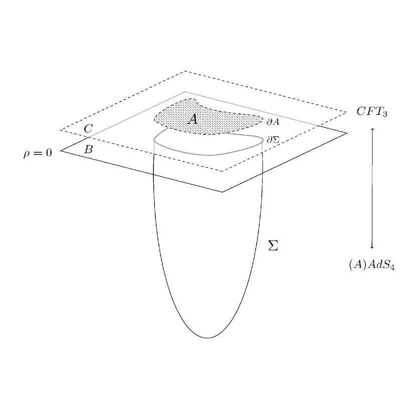
Figure 1: In this diagram, we show all the submanifolds involved in the RT construction. On the field theory side, $C$ is the conformal boundary where the CFT is defined, $A$ is the entangling region and $\partial A$ is the entangling surface. On the gravity side, $B$ is the boundary of spacetime, $\Sigma$ is the minimal surface in the bulk and $\partial\Sigma$ is its border at the spacetime boundary. Both sides are related such that $C$ is conformal to $B$ and $\partial A$ is conformal to $\partial\Sigma$.

This definition for the EE is formally divergent, due to the presence of an infinite conformal factor at the AdS boundary $B$, what is manifest in the Fefferman-Graham (FG) form of the metric FeffermanGraham Imbimbo . As it was shown by Taylor and Woodhead Marika , it is possible to renormalize the EE by adding counterterms constructed through the Replica Trick EECovariant -Marika from the standard Holographic Renormalization procedure UsualCounterJohnson -SkenderisAndPapa2 . This is done by evaluating the usual counterterms for Einstein gravity at the conically singular spacetime boundary, which is conformal to the manifold of the Replica CFT.

Here, we propose an alternative regularization prescription that has the advantage of giving the countertem for the EE as a single boundary term, which can be written in closed form for CFTs of arbitrary (odd) dimensions that have an (even-dimensional) AAdS E-H gravity dual. This boundary term corresponds to the Chern form evaluated at the boundary of the RT minimal surface, which is conformal to the entangling surface that bounds the entangling region in the CFT. In particular, we propose that the renormalized EE of a 3D CFT with a 4D AAdS E-H gravity dual is given by

$$S_{EE}^{ren}=\frac{Vol\left(\Sigma\right)}{4G}+\frac{\ell^{2}}{8G}\int\limits_{\partial\Sigma}B_{1},$$ (1)

where $\Sigma$ is the codimension-2 RT minimal surface, $\partial\Sigma$ is its border at the spacetime boundary $B$, $\ell$ is the AdS radius. In addition, $B_{1}$ is the first Chern form evaluated at the border of the RT minimal surface, whose detailed form is given in eq.(33). Therefore, we show that the EE counterterm ($S_{EE}^{ct}$) is given by the $B_{1}$ term, which depends on the induced metric $\widetilde{\gamma}$ of $\partial\Sigma$, and on its extrinsic curvature with respect to the radial foliation along the holographic radial coordinate $\rho$, which is the parameter of the FG expansion. It is apparent then, that the Chern form is written in terms of both intrinsic and extrinsic quantities of $\partial\Sigma$. The particular features of $S_{EE}^{ct}$ are explained in section III.

In order to obtain the EE boundary counterterm, we consider the Replica Trick, where the conically singular replica manifold is constructed as described in RenyiXiDong . We also consider the gravitational Euclidean action in the AAdS bulk. The EE is then expressed in terms of a derivative of said action evaluated on the replica manifold, with respect to the conical angular parameter. Therefore, if the action is itself renormalized, the EE computed in this manner will be renormalized as well. In order to renormalize the bulk gravitational action, we consider the Kounterterms proposal K1Even -KounterComparison2 , instead of the standard Holographic Renormalization prescription UsualCounterJohnson -SkenderisAndPapa2 . This choice is made because of the fact that in the Kounterterms scheme, the counterterm that renormalizes the on-shell gravitational action can be written in closed form, as a single boundary term with topological origin. As a matter of fact, this prescription is known for arbitrary dimensions and also for any gravity theory of Lovelock type. For the evaluation of the renormalized action on the replica manifold, we consider a generalization of the Euler theorem to conically singular manifolds in 4D, derived by using distributional geometry Solodukhin1 SolodukhinNew . Thus, the counterterm of the action splits into a regular part at the spacetime boundary and another at $\partial\Sigma$. The latter results in a contribution proportional to the angular parameter which gives the $B_{1}$ piece of eq.(1). Upon taking the derivative of the action with respect to the conically singular parameter, we obtain $S_{EE}^{ren}$ as shown in eq.(1), where the bulk part of the action gives the usual RT term. We emphasize that the form of $S_{EE}^{ren}$ obtained in the AdS₄/CFT₃ case, and shown in eq.(1), is equivalent to the known result of

$$S_{EE}^{ren}=\frac{Vol\left(\Sigma\right)}{4G}-\frac{\ell}{4G}\int\limits_{\partial\Sigma}dx\sqrt{\widetilde{\gamma}},$$ (2)

given in Marika , as explained in section III.2.

This paper is organized as follows: In section II, we explain the setup used for obtaining the renormalized EE. We give a general overview of the definition of EE and of the Replica Trick, applied to the AdS/CFT context. We then explain the generalization of the Euler theorem for conically singular manifolds, and in particular, for the case without a $U\left(1\right)$ isometry in 4D. Then, we introduce the renormalized Euclidean gravitational action obtained by the Kounterterms procedure. In section III, we use the elements described in the setup to obtain the $S_{EE}^{ct}$ in the AdS₄/CFT₃ case. We also expand the obtained boundary counterterm considering the explicit covariant embedding of the $\Sigma$ minimal surface on the bulk. When taking the FG expansion of its induced metric we show that $S_{EE}^{ct}$ can be re-written in the standard way of eq.(2). We explicitly check the finiteness of $S_{EE}^{ren}$, and we verify that the standard computation of the renormalized EE of a disc-like entangling region in CFT₃ is correctly recovered. We also give a new interpretation of $S_{EE}^{ren}$ in terms of the topological and geometrical properties of the minimal surface $\Sigma$ as an AAdS submanifold (see eq.(47)). Finally, in section IV, we give a general outlook of the method and comment on possible generalizations thereof.

II The setup: Replica trick and renormalized Euclidean action in the conically singular manifold

We proceed to explain the different elements of the setup considered in order to obtain the renormalized entanglement entropy $S_{EE}^{ren}$. We start by giving a brief overview of EE in the AdS/CFT context, discussing how to compute it with the replica trick, in terms of derivatives of the on-shell Euclidean action. Then, we explain the generalization of the Euler theorem to 4D conically singular manifolds without $U\left(1\right)$ isometry. Finally, we consider the renormalized Euclidean gravitational E-H action, as obtained by the Kounterterms procedure, and comment on its properties and usefulness for the computation of $S_{EE}^{ren}$.

II.1 Entanglement Entropy and replica trick

The EE RT1 -Maldacena1 is defined as the von Neumann entropy of the reduced density matrix of a quantum subsystem $A$, i.e.

$$S_{EE}=-Tr\left(\widehat{\rho}_{A}\ln\widehat{\rho}_{A}\right),$$ (3)

and it encodes the degree of entanglement of the subsystem $A$ with the rest of the system ($A^{c}$). The first proposal for computing EEs of CFTs in the AdS/CFT framework was the RT formula RT1 . Said formula states that the EE of an entangling region $A$ in a (D-1)-dimensional CFT with a D-dimensional AAdS gravity dual is equal to the volume of a codimension 2 minimal hypersurface ($\Sigma$) in the AAdS bulk whose border is conformal to the one of the entangling region ($A$) at the conformal boundary; i.e., $S_{EE}=\frac{Vol(\Sigma)}{4G}$ (in natural units). This formula is analogous to the Bekenstein-Hawking entropy formula for a black hole BHE1 -BHE3 , and it was shown (e.g., by Lewkowycz and Maldacena in Maldacena1 ) that indeed both formulas can be obtained from the replica trick EECovariant -Marika .

The computation of the EE by the replica trick considers that eq.(3) can be re-written as

$$S_{EE}=\lim_{n\rightarrow 1}-\frac{1}{n-1}\ln(Tr\left(\widehat{\rho}_{A}^{n}\right)),$$ (4)

and therefore, the EE is expressed in terms of the trace of the n-th power of the reduced density matrix. In order to compute this trace, one constructs a branched cover of the conformal boundary $C$ where the CFT is defined. This is achived by gluing together n copies of the original (Euclideanized) boundary with a cut along the entangling region whose EE is being computed RenyiXiDong . The gluing is done such that, when defining an angular coordinate that circles around the border of the entangling region, after $2\pi$ rotations along the coordinate, the copies are cyclically permuted. Labelling this branched cover manifold as $C_{n}$, one realizes that it has a $Z_{n}$ symmetry corresponding to cycling from one copy (replica) of the CFT to another. Finally, one defines the orbifold $\widehat{C}_{n}$ as the quotient of the cover manifold by the permutation symmetry, i.e., $\widehat{C}_{n}=C_{n}/Z_{n}$. The orbifold $\widehat{C}_{n}$ is conically singular, with an opening angle of $\frac{2\pi}{n}$. However, because the permutation symmetry is the discrete symmetry $Z_{n}$, the orbifold does not have a $U\left(1\right)$ isometry in general.

Considering the $\widehat{C}_{n}$ orbifold, $Tr\left(\widehat{\rho}_{A}^{n}\right)$ can be computed in terms of the partition function of the replica CFT defined on the orbifold, as

$$Tr\left(\widehat{\rho}_{A}^{n}\right)=n\left(\ln\left(Z\left(\widehat{C}_{n}\right)\right)-\ln\left(Z\left(\widehat{C}_{1}\right)\right)\right),$$ (5)

where $\widehat{C}_{1}$ (which is equal to $C$) is the manifold of the original CFT and $Z\left(\widehat{C}_{1}\right)$ is its partition function.

One then defines the orbifold $\widehat{M}_{n}$ as the extension of $\widehat{C}_{n}$ into the AAdS bulk, by requiring the bulk metric to be a solution of the equations of motion. Because the orbifold $\widehat{M}_{n}$ is a solution in the bulk, the semi-classical approximation can be used to write the partition functions in eq(5) in terms of the corresponding gravitational Euclidean on-shell actions in the AAdS bulk (including boundary terms). Then, in the saddle-point approximation, one has that $\ln(Z(\widehat{C}_{n}))=-I_{E}(\widehat{M}_{n})$, and therefore,

$$Tr\left(\widehat{\rho}_{A}^{n}\right)=-n\left(I_{E}(\widehat{M}_{n})-I_{E}(\widehat{M}_{1})\right).$$ (6)

Thus, in the AdS/CFT context, the EE computed by the replica trick can be written as

$$S_{EE}=\lim_{n\rightarrow 1}\frac{n}{n-1}(I_{E}(\widehat{M}_{n})-I_{E}(\widehat{M}_{1}))=\left.n^{2}\partial_{n}I_{E}\left(\widehat{M}_{n}\right)\right|_{n=1}.$$ (7)

Finally, for ease of computation, we define the angular parameter $\alpha$ such that $\alpha=\frac{1}{n},$ where the cone then has an angular deficit given by $2\pi\left(1-\alpha\right)=2\pi\left(1-\frac{1}{n}\right)$. Thus, in the case of a 3D CFT with a 4D AAdS gravity dual, the EE is

$$S_{EE}=\left.-\partial_{\alpha}I_{E}\left(\widehat{M}_{4}^{(\alpha)}\right)\right|_{\alpha=1},$$ (8)

where now $\widehat{M}_{4}^{(\alpha)}$ denotes the 4D orbifold with angular deficit given by $2\pi\left(1-\alpha\right)$.

In order to evaluate this Euclidean action, we first need to discuss some properties of differential geometry in conically singular manifolds Solodukhin1 -Cone3 . In particular, in the next section, we review a generalization of the Euler theorem for squashed cones (conically singular manifolds without $U\left(1\right)$ isometry) in 4D.

II.2 Euler theorem for conically singular manifolds in 4D

In differential geometry, topological invariants are interesting because they characterize properties of manifolds that are robust under continuous deformations of their metric. For example, the Euler characteristic in $D=2m$ can be written as the integral of a precise combination of a product of $m-$curvature terms, with the addition of the $m-$th Chern form in a manifold with boundaries. The Chern form is expressible considering both intrinsic and extrinsic curvatures of the boundary’s induced metric. Therefore, this way of writing the Euler characteristic provides a global relation between the curvature of a bulk manifold, and the curvatures of its boundary. In particular, the Euler theorem K1Even , which is valid for $2m-$dimensional manifolds, states that

$$\int\limits_{M_{2m}}\varepsilon_{2m}=\left(4\pi\right)^{m}m!\chi\left(M_{2m}\right)+\int\limits_{\partial M_{2m}}B_{2m-1},$$ (9)

where $\varepsilon_{2m}$ is the Euler density in $2m$ dimensions, $\chi\left(M_{2m}\right)$ is the Euler characteristic of the manifold $M_{2m}$, and $B_{2m-1}$ is the $m-$th Chern form at the boundary of the manifold. In the particular case of $m=2$, and therefore $\dim\left(M_{2m}\right)=4$, the Euler density $\varepsilon_{4}$ is the usual Gauss-Bonnet term and $B_{3}$ is the second Chern form (given in eq.(20) in Gauss normal coordinates).

As we will see in section III, in order to obtain the renormalized version of $S_{EE}$, we need to evaluate either $\varepsilon_{4}$ or $B_{3}$ on conically singular manifolds (without $U\left(1\right)$ rotational isometry). To this end, we consider the results obtained by Fursaev, Patrushev and Solodukhin (FPS) SolodukhinNew regarding the computation of quadratic terms in the curvature, for conically singular manifolds in 4D.

In order to compute the integral of the quadratic terms, which correspond to the Ricci scalar squared, the Ricci tensor squared and the Riemann tensor squared, FPS used the methods of distributional geometry, as described in Solodukhin1 SolodukhinNew . There, a conically singular orbifold was considered as the limit of a sequence of regular manifolds whose metrics are parametrized by a certain regularization parameter. Then, the quadratic terms are computed, and the parameter is taken to zero, in order to recover the conically singular manifold (for further details, we refer the reader to the original papers).

In particular, FPS obtained that the integral of the square of the Riemann tensor evaluated on the 4D orbifold $\widehat{M}_{4}^{\left(\alpha\right)}$ is given by

$$\begin{array}[c]{c}{\displaystyle\int\limits_{\widehat{M}_{4}^{\left(\alpha\right)}}}d^{4}x\sqrt{G}\left(R^{\left(\alpha\right)}\right)_{\nu\sigma\lambda}^{\mu}\left(R^{\left(\alpha\right)}\right)_{\mu}^{\nu\sigma\lambda}={\displaystyle\int\limits_{M_{4}}}d^{4}x\sqrt{G}\left(R^{\left(r\right)}\right)_{\nu\sigma\lambda}^{\mu}\left(R^{\left(r\right)}\right)_{\mu}^{\nu\sigma\lambda}+\\ 8\pi\left(1-\alpha\right){\displaystyle\int\limits_{\Sigma}}d^{2}x\sqrt{\gamma}\left(R_{\left(i\right)\left(j\right)\left(i\right)\left(j\right)}^{\left(r\right)}-\left(K_{\left(i\right)}\right)_{b}^{a}\left(K_{\left(i\right)}\right)_{a}^{b}\right)+O\left(\left(1-\alpha\right)^{2}\right),\end{array}$$ (10)

where $\left(R^{\left(\alpha\right)}\right)_{\nu\sigma\lambda}^{\mu}$ denotes the bulk Riemann tensor evaluated on the orbifold, $\left(R^{\left(r\right)}\right)_{\nu\sigma\lambda}^{\mu}$ represents the regular part of the bulk Riemann tensor, $M_{4}$ refers to the regular manifold given in the $\alpha\rightarrow 1$ limit (where $2\pi\left(1-\alpha\right)$ is the angular deficit of the cone), $G_{\mu\nu}$ corresponds to the bulk metric of the manifold, $\Sigma$ is the codimension-2 surface located at the tip of the cone and given by the fixed-point set of the $Z_{n}$ symmetry of the orbifold, $\gamma_{ab}$ is the induced metric on $\Sigma$, $R_{\left(i\right)\left(j\right)\left(i\right)\left(j\right)}^{\left(r\right)}$ denotes the corresponding components of the Riemann tensor where $\left(i\right)$ and $\left(j\right)$ are the indices of the foliation ($i,j=1,2$) and $\left(K_{\left(i\right)}\right)_{b}^{a}$ is the extrinsic curvature tensor of the surface $\Sigma$ with respect to the $i-$th direction of the foliation that is normal to the surface ($i=1,2$), where a sum over repeated foliation indices is implied. We note that$\left(R^{\left(\alpha\right)}\right)_{\alpha\beta}^{\mu\nu}$ is divergent at $\Sigma$, and it can be written as

$$\left(R^{\left(\alpha\right)}\right)_{\sigma\lambda}^{\mu\nu}=\left(R^{\left(r\right)}\right)_{\sigma\lambda}^{\mu\nu}+2\pi\left(1-\alpha\right)\left(N_{\sigma\lambda}^{\mu\nu}+T_{\sigma\lambda}^{\mu\nu}\right)\delta_{\Sigma},$$

     (11)

where $\delta_{\Sigma}$ is a codimension-2 delta function which only has support on $\Sigma$, $\left(n_{\left(i\right)}\right)_{\mu}$ is the $i-$th normal vector to the $\Sigma$ surface ($i=1,2$) and $T_{\sigma\lambda}^{\mu\nu}$ is a tensor which depends on the extrinsic curvatures of $\Sigma$ with respect to the two directions of the foliation. In the case that the cone has a $U\left(1\right)$ rotational symmetry, $T_{\sigma\lambda}^{\mu\nu}=0$. However in our case, although $T_{\sigma\lambda}^{\mu\nu}$ is left unspecified, it does encode the extrinsic curvature contributions to the quadratic terms.

Analogously, FPS obtained that for the square of the Ricci tensor,

$$\begin{array}[c]{c}{\displaystyle\int\limits_{\widehat{M}_{4}^{\left(\alpha\right)}}}d^{4}x\sqrt{G}\left(R^{\left(\alpha\right)}\right)_{\mu\nu}\left(R^{\left(\alpha\right)}\right)^{\mu\nu}={\displaystyle\int\limits_{M_{4}}}d^{4}x\sqrt{G}\left(R^{\left(r\right)}\right)_{\mu\nu}\left(R^{\left(r\right)}\right)^{\mu\nu}+\\ 4\pi\left(1-\alpha\right){\displaystyle\int\limits_{\Sigma}}d^{2}x\sqrt{\gamma}\left(R_{\left(i\right)\left(i\right)}^{\left(r\right)}-\frac{1}{2}\left(K_{\left(i\right)}\right)_{a}^{a}\left(K_{\left(i\right)}\right)_{b}^{b}\right)+O\left(\left(1-\alpha\right)^{2}\right),\end{array}$$ (12)

and for the square of the Ricci scalar,

$${\displaystyle\int\limits_{\widehat{M}_{4}^{\left(\alpha\right)}}}d^{4}x\sqrt{G}\left(R^{\left(\alpha\right)}\right)^{2}={\displaystyle\int\limits_{M_{4}}}d^{4}x\sqrt{G}\left(R^{\left(r\right)}\right)^{2}+8\pi\left(1-\alpha\right){\displaystyle\int\limits_{\Sigma}}d^{2}x\sqrt{\gamma}\left(R^{\left(r\right)}\right)+O\left(\left(1-\alpha\right)^{2}\right).$$ (13)

Because in the computation of $S_{EE}$ we need to take the $\alpha\rightarrow 1$ limit, it is safe to neglect terms of quadratic or higher order in $\left(1-\alpha\right)$.

Finally, we have that the Gauss-Codazzi decomposition of the regular part of the Ricci scalar on $M_{4}$ gives

$$R^{\left(r\right)}=-R_{\left(i\right)\left(j\right)\left(i\right)\left(j\right)}^{\left(r\right)}+2R_{\left(i\right)\left(i\right)}^{\left(r\right)}+\mathcal{R}-\left(K_{\left(i\right)}\right)_{a}^{a}\left(K_{\left(i\right)}\right)_{b}^{b}+\left(K_{\left(i\right)}\right)_{a}^{b}\left(K_{\left(i\right)}\right)_{b}^{a},$$ (14)

where we $\mathcal{R}$ is the intrinsic Ricci scalar at the surface $\Sigma$ (computed with the induced metric $\gamma_{ab}$), and the other quantities have the same meaning as for the quadratic terms presented above.

Now, considering eqs.(10-14), we evaluate $\varepsilon_{4}$ on the $\widehat{M}_{4}^{\left(\alpha\right)}$ orbifold. The Gauss-Bonnet term is given by

$$\varepsilon_{4}=\sqrt{G}d^{4}x\left(R_{\nu\sigma\lambda}^{\mu}R_{\mu}^{\nu\sigma\lambda}-4R_{\mu\nu}R^{\mu\nu}+R^{2}\right),$$ (15)

and therefore, we obtain that

$$\int\limits_{\widehat{M}_{4}^{\left(\alpha\right)}}\varepsilon_{4}^{\left(\alpha\right)}=\int\limits_{M_{4}}\varepsilon_{4}^{\left(r\right)}+8\pi\left(1-\alpha\right)\int\limits_{\Sigma}\varepsilon_{2}+O\left(\left(1-\alpha\right)^{2}\right),$$ (16)

where we used that $\varepsilon_{2}=\mathcal{R}\sqrt{\gamma}d^{2}x$ is the usual 2D Gauss-Bonnet term, which depends on the intrinsic Ricci scalar at the surface $\Sigma$.

Furthermore, considering that (as shown in FPS) for squashed-cone manifolds in 4D, the Euler characteristic obeys the relation

$$\chi_{4}\left(\widehat{M}_{4}^{\left(\alpha\right)}\right)=\chi_{4}\left(M_{4}\right)+\left(1-\alpha\right)\chi_{2}\left(\Sigma\right)+O\left(\left(1-\alpha\right)^{2}\right),$$ (17)

and also using eq.(9) for the $m=1$ and $m=2$ cases, we obtain that the boundary terms (given by the corresponding Chern forms) are related by

$$\int\limits_{\partial\widehat{M}_{4}^{\left(\alpha\right)}}B_{3}^{\left(\alpha\right)}=\int\limits_{\partial M_{4}}B_{3}^{\left(r\right)}+8\pi\left(1-\alpha\right)\int\limits_{\partial\Sigma}B_{1}+O\left(\left(1-\alpha\right)^{2}\right),$$ (18)

where $B_{1}$ is evaluated at the boundary of the codimension-2 surface $\Sigma$.

It is precisely this last relation which will be used in section III, in order to evaluate the Euclidean action in the orbifold, which will ultimately give the expression for the renormalized EE when considering the renormalized Euclidean action which will be discussed in the following subsection.

II.3 Renormalized Euclidean action and Topological Invariants

In order to obtain a renormalized version of eq.(8), to be able to compute the finite part of the EE, we need to consider a suitably renormalized Euclidean action for the bulk gravity theory.

For AAdS spacetimes, there are different prescriptions for renormalizing the Euclidean on-shell action. The standard Holographic Renormalization method consists on adding counterterms to the action as surface terms, UsualCounterJohnson -SkenderisAndPapa2 . In doing so, the divergences occuring due to the presence of the infinite conformal factor in the metric at the boundary, as seen in its Fefferman-Graham expansion FeffermanGraham are cancelled out. The counterterms are functionals of the boundary metric, its intrinsic curvature and covariant derivatives thereof, in order to be consistent with a well posed variational principle for the conformal class of spacetimes $\left[h_{ij}\right]$ at the boundary SkenderisAndPapa1 SkenderisAndPapa2 , after the Gibbons-Hawking-York term is included. Although there is a systematic procedure for computing the counterterms, in principle, at any order in the holographic radial coordinate $\rho$ and for any number of spacetime dimensions DirichletKraus(quasiloc) , the number of counterterms required grows rapidly with the dimension. Furthermore, the functional form of the terms in the series is different for different gravity actions including higher-curvature theories (e.g., Lovelock gravity theories).

The Kounterterms procedure, developed in ref.K1Even , and further understood in ref.KounterComparison2 , consists on adding a given boundary term to the AdS gravity action in order to both attain a well defined variational principle and to render the action finite. The particular term that is added is universal for all gravity theories of Lovelock type and depends only on the number of dimensions of spacetime and on whether said number is odd or even. In the case of AAdS spacetimes in even dimensions, with $D=2m$, the term added is the $m-$th Chern form K1Even . For odd-dimensional spacetimes, the term added corresponds to the boundary term of the Chern-Simons transgression form of the AdS group K2Odd . In both cases, the added boundary term depends on both the intrinsic and extrinsic ($K_{j}^{i}$) curvatures of the boundary in the radial foliation of the spacetime, and hence the name Kounterterms. Therefore, it is easy to particularize to the case of Fefferman-Graham expansion (with respect to the holographic radial coordinate $\rho$). In even-dimensional manifolds, there is a relation between the added boundary terms and topological terms. Indeed, the $m-$th Chern form is the boundary term associated with the Euler theorem, which relates the integral of the Euler term in the bulk with the Euler characteristic of the manifold, as mentioned in the previous subsection.

It is important to note that in KounterComparison KounterComparison2 , it was proven that the addition of Kounterterms is equivalent to the standard Holographc Renormalization procedure in Einstein gravity in even dimmensions. As a matter of fact, standard counterterms are recovered when expressing these extrinsic counterterms in terms of the intrinsic curvature at the boundary (making extensive use of the FG expansion for $K_{j}^{i}$ ), order by order in the holographic radial coordinate $\rho$. However, the universality of the Kounterterms method with respect to different gravity theories (i.e., all theories of Lovelock type) and the fact that the closed-form expression for the boundary term is known for any dimension are its main practical advantages over the standard Holographic Renormalization procedure; but also its relation to topology is interesting on its own.

In this paper, we consider the renormalized action given by the Kounterterms prescription, which for the case of EH gravity in 4D AAdS manifolds is given by K1Even

$$I_{E}^{ren}=\frac{1}{16\pi G}\left({\displaystyle\int\limits_{M_{4}}}d^{4}x\sqrt{G}\left(R-2\Lambda\right)+\frac{\ell^{2}}{4}{\displaystyle\int\limits_{\partial M_{4}}}B_{3}\right),$$ (19)

where $\Lambda=-\frac{3}{\ell^{2}}$, and $B_{3}$ is given by

$$B_{3}=-4\int_{0}^{1}dtd^{3}x\sqrt{h}\delta_{[i_{1}i_{2}i_{3}]}^{[j_{1}j_{2}j_{3}]}K_{j_{1}}^{i_{1}}\left(\frac{1}{2}\mathcal{R}_{j_{2}j_{3}}^{i_{2}i_{3}}-t^{2}K_{j_{2}}^{i_{2}}K_{j_{3}}^{i_{3}}\right).$$ (20)

In eq.(20), $h_{ij}$ is the metric at the boundary of spacetime, $\mathcal{R}_{ij}^{k\ell}$ is the Riemann curvature tensor at the boundary, computed with the $h_{ij}$ metric, and $K_{j}^{i}$ is the extrinsic curvature tensor of the boundary with respect to a radial foliation along the holographic radial coordinate $\rho$. The main reason for adopting this renormalization scheme is that the boundary term $B_{3}$ can be directly evaluated in the orbifold $\widehat{M}_{4}^{\left(\alpha\right)}$ using the generalized Euler theorem for the boundary terms, as presented in eq.(18). Then, the counterterm for the renormalized EE directly becomes the $B_{1}$ term evaluated at the entangling surface $\partial\Sigma$ as shown in eq.(1). This will be explained in detail in the following section.

III Renormalization of EE in AdS₄/CFT₃ through the Chern form

After introducing the renormalized Euclidean action for the dual gravitational theory and also the generalization of the Euler theorem for 4D squashed-cone manifolds, we proceed to compute the renormalized EE $\left(S_{EE}^{ren}\right)$ by means of the replica trick. This is done by evaluating eq.(8) using the renormalized gravitational action of eq.(19). This assumes that if the gravitational action is itself renormalized, then the resulting EE will be renormalized as well.

The renormalized Euclidean on-shell action, evaluated on the conically singular manifold $\widehat{M}_{4}^{(\alpha)}$, is given by

$$I_{E}^{ren}=\frac{1}{16\pi G}\left({\displaystyle\int\limits_{\hat{M}_{4}^{\left(\alpha\right)}}}d^{4}x\sqrt{G}\left(R^{\left(\alpha\right)}-2\Lambda\right)+\frac{\ell^{2}}{4}{\displaystyle\int\limits_{\partial\hat{M}_{4}^{\left(\alpha\right)}}}B_{3}^{\left(\alpha\right)}\right).$$ (21)

As it was discussed by Lewkowicz and Maldacena Maldacena1 and by Dong RenyiXiDong , the Einstein-Hilbert part of eq.(21) gives the usual RT area formula for the EE, when computing the derivative of eq.(8) with respect to the conical angle parameter $\alpha$. Therefore, the counterterm that regularizes the EE will come from the $B_{3}^{\left(\alpha\right)}$ part. We defne the counterterm of the Euclidean action as

$$I_{E}^{ct}=\frac{\ell^{2}}{64\pi G}{\displaystyle\int\limits_{\partial\hat{M}_{4}^{\left(\alpha\right)}}}B_{3}^{\left(\alpha\right)},$$ (22)

and therefore, we proceed to compute the counterterm of the EE ($S_{EE}^{ct}$) as

$$S_{EE}^{ct}=\left.-\partial_{\alpha}I_{E}^{ct}\left(\partial\widehat{M}_{4}^{(\alpha)}\right)\right|_{\alpha=1},$$ (23)

such that $S_{EE}^{ren}=S_{EE}^{RT}+S_{EE}^{ct}$, where $S_{EE}^{RT}$ is the usual RT prescription for the EE.

Using eq.(18) to evaluate $I_{E}^{ct}$, we have that

$$S_{EE}^{ct}=\frac{\ell^{2}}{8G}\int\limits_{\partial\Sigma}B_{1},$$ (24)

and therefore, we recover the expression for $S_{EE}^{ren}$ given in eq.(1).

In the next subsections, we will expand the integrands of $S_{EE}^{ren}$ in their corresponding FG expansions, in order to verify the finiteness of the renormalized EE, and also in order to show that our result is equivalent to the one obtained in Marika . We will also compute $S_{EE}^{ren}$ for the particular case of a disk-like entangling region in the 3D CFT, with a global AdS₄ gravitational dual (corresponding to the ground state of the CFT). In order to do this, we will consider the explicit embedding of the minimal surface $\Sigma$ and its boundary $\partial\Sigma$, as given in HungMyersSmolkin SchwimmerAndTheisen and as explained in what follows.

III.1 Explicit covariant embedding

Following the works by Hung, Myers and Smolkin HungMyersSmolkin , and by Schwimmer and Theisen SchwimmerAndTheisen we consider that the embedding of the minimal surface $\Sigma$ on the bulk is given by

$$x^{i}\left(\tau,y^{a}\right)=\left(x^{\left(0\right)}\right)^{i}\left(y^{a}\right)+\tau\left(x^{\left(2\right)}\right)^{i}\left(y^{a}\right)+...$$

     (25)

where $\left\{\rho,x^{i}\right\}$ are bulk coordinates and $\left\{\tau,y^{a}\right\}$ are coordinates on the worldvolume of $\Sigma$.

We label the AAdS bulk metric as $G_{\mu\nu}$ and the metric at the spacetime boundary as $h_{ij}$. Analogously, we label the induced metric on $\Sigma$ as $\gamma_{ab}$ and the induced metric on its boundary ($\partial\Sigma$) as $\widetilde{\gamma}_{ab}$. As it is well known (see, e.g., Imbimbo ), the metric $G_{\mu\nu}$ has a FG expansion FeffermanGraham given by

$$ds_{G}^{2}=G_{\mu\nu}dx^{\mu}dx^{\nu}=\frac{\ell^{2}d\rho^{2}}{4\rho^{2}}+h_{ij}\left(\rho,x\right)dx^{i}dx^{j},$$

   (26)

where $\rho$ is the holographic radial coordinate (the spacetime boundary is located at $\rho=0$).

Now, the induced metric $\gamma_{ab}$ is defined as

$$\gamma_{ab}=\frac{\partial x^{\mu}}{\partial y^{a}}\frac{\partial x^{\nu}}{\partial y^{b}}G_{\mu\nu},$$ (27)

and upon choosing the diffeomorphism gauge as $\tau=\rho$ and $\gamma_{a\tau}=0$, one obtains that

$$ds_{\gamma}^{2}=\gamma_{ab}dy^{a}dy^{b}=\frac{\ell^{2}}{4\tau^{2}}\left(1+\frac{\tau\ell^{2}}{\left(d-2\right)^{2}}\kappa^{i}\kappa^{j}g_{ij}^{\left(0\right)}+...\right)d\tau^{2}+\widetilde{\gamma}_{ab}\left(\tau,y\right)dy^{a}dy^{b},$$

     (28)

which has the form of a FG-like expansion for the induced metric on $\Sigma$. To make this last statement more precise, $\gamma_{ab}$ is given by the pullback onto $\Sigma$ of the $G_{\mu\nu}$ bulk metric in the FG gauge.

We now explain the meaning of the coefficients in the FG expansions of the previous equations. In particular, $d$ is the dimension of the boundary of spacetime ($d=3$ in our case), $g_{ij}^{\left(0\right)}$ is the metric at the conformal boundary (where the 3D CFT is defined) and $\sigma_{ab}^{\left(0\right)}$ is the induced metric on the entangling surface $\partial A$ (embedded in the conformal boundary) which is given by

$$\sigma_{ab}^{\left(0\right)}=\frac{\partial\left(x^{\left(0\right)}\right)^{i}}{\partial y^{a}}\frac{\partial\left(x^{\left(0\right)}\right)^{j}}{\partial y^{b}}g_{ij}^{\left(0\right)}.$$ (29)

Furthermore, $g_{ij}^{\left(2\right)}=-\ell^{2}S_{ij}^{\left(0\right)}$ where $S_{ij}^{\left(0\right)}$ is the Schouten tensor of the $g_{ij}^{\left(0\right)}$ metric given by

$$\left(S^{\left(0\right)}\right)_{ij}=\frac{1}{\left(d-2\right)}\left(R_{ij}^{\left(0\right)}-\frac{g_{ij}^{\left(0\right)}}{2\left(d-1\right)}R^{\left(0\right)}\right),$$ (30)

and $\sigma_{ab}^{\left(2\right)}$ is given by

$$\sigma_{ab}^{\left(2\right)}=\frac{\partial\left(x^{\left(0\right)}\right)^{i}}{\partial y^{a}}\frac{\partial\left(x^{\left(0\right)}\right)^{j}}{\partial y^{b}}g_{ij}^{\left(2\right)}-\frac{\ell^{2}}{\left(d-2\right)}\kappa^{i}\kappa_{ab}^{j}\left(g^{\left(0\right)}\right)_{ij}.$$ (31)

Finally,

$$\kappa^{i}=\hat{n}_{\left(n\right)}^{i}\kappa_{ab}^{\left(n\right)}\left(\sigma^{\left(0\right)}\right)^{ab},$$ (32)

where the extrinsic curvatures $\kappa_{ab}^{\left(n\right)}$ are defined with respect to the foliation that is normal to $\partial A$ (which is conformal to $\partial\Sigma$) embedded in the conformal boundary (which is conformal to the boundary of spacetime), and $\hat{n}_{\left(n\right)}^{i}$ are the vectors along the directions of the foliation ($n=1,2$).

Having introduced the explicit covariant embedding of $\Sigma$ in $\widehat{M}_{4}^{(\alpha)}$, and the corresponding FG expansions of $G_{\mu\nu}$ and $\gamma_{ab}$, we now proceed to show that $S_{EE}^{ren}$, as defined in eq.(1), is finite and equivalent to the standard expression given in eq.(2), and first obtained in Marika .

III.2 Proof of finiteness of $S_{EE}^{ren}$

With the previously considered embedding, we can check the cancellation of divergences in $S_{EE}^{ren}$ for 3D CFTs with 4D AAdS gravity duals. We note that the explicit value of $S_{EE}^{ren}$ depends on the shape of the entangling surface $\partial A$ at the conformal boundary. Here, we simply exhibit the divergences in $S_{EE}^{RT}$ (the standard Ryu-Takayanagi EE) and check that they are exactly cancelled by $S_{EE}^{ct}$ (the EE counterterm given in eq.(24)). This cancellation is independent of the shape of $\partial A$.

In particular, we have

$$B_{1}=-2dy\sqrt{\widetilde{\gamma}}\delta_{a}^{b}k_{b}^{a},$$

       (33)

where $k_{ab}$ is the extrinsic curvature of $\partial\Sigma$ with respect to the radial foliation along the holographic radial coordinate $\rho$ (not to be confused with $\kappa_{ab}^{\left(n\right)}$ for $\partial A$, or with $K_{ij}$ for $B$).

Now, we consider the FG expansion of each of the pieces. From eq.(28), we have that the square root of the determinant of the metric on $\Sigma$ and on $\partial\Sigma$ are given, respectively, by

$$\sqrt{\gamma}=\frac{\ell\sqrt{\sigma^{\left(0\right)}}}{2\rho^{d/2}}\left(1+\rho\left[\frac{\ell^{2}}{2\left(d-2\right)^{2}}\kappa^{i}\kappa^{j}g_{ij}^{\left(0\right)}+\frac{1}{2}tr[\sigma^{\left(2\right)}]\right]+...\right),$$

       (34)

where $tr[\sigma^{\left(2\right)}]$ denotes the trace of the $\sigma_{ab}^{\left(2\right)}$ tensor, given in the paragraph following eq.(28). Also, $\widetilde{\gamma}^{ab}$ is the inverse of the induced metric on $\partial\Sigma$, and it is given by $\widetilde{\gamma}^{ab}=\rho\left(\left(\sigma^{\left(0\right)}\right)^{ab}-\rho\left(\sigma^{\left(2\right)}\right)^{ab}+...\right)$. Now, considering the FG-like expansion of the induced metric on $\Sigma$, the extrinsic curvature $k_{ab}$ with respect to the radial foliation is computed, by definition, as $k_{ab}=\frac{-1}{2\sqrt{\gamma_{\rho\rho}}}\partial_{\rho}\widetilde{\gamma}_{ab}$. Thus, we have that

$$k_{ab}=\frac{\sigma_{ab}^{\left(0\right)}}{\ell\rho}\left(1-\frac{\rho\ell^{2}}{2\left(d-2\right)^{2}}\kappa^{i}\kappa^{j}g_{ij}^{\left(0\right)}+...\right).$$ (35)

Finally, in order to evaluate $S_{EE}^{ct}$, we consider the expansion of $\sqrt{\widetilde{\gamma}}\widetilde{\gamma}^{ab}k_{ab}$ at the cutoff $\rho=\varepsilon$, where the limit of $\varepsilon\rightarrow 0$ has to be evaluated at the end. Thus, we have

$$\left.\sqrt{\widetilde{\gamma}}\widetilde{\gamma}^{ab}k_{ab}\right|_{\rho=\varepsilon}=\frac{\left(d-2\right)\sqrt{\sigma^{\left(0\right)}}}{\ell\varepsilon^{\left(d-2\right)/2}}\left(1+\varepsilon\left[\frac{\left(d-4\right)}{2\left(d-2\right)}tr\left[\sigma^{\left(2\right)}\right]-\frac{\ell^{2}}{2\left(d-2\right)^{2}}\kappa^{i}\kappa^{j}g_{ij}^{\left(0\right)}\right]+...\right).$$ (36)

Now we have all the pieces required to check that the divergences of $S_{EE}^{ren}$ vanish. We therefore consider that

$$S_{EE}^{RT}=\frac{1}{4G}\int\limits_{\Sigma}d^{2}y\sqrt{\gamma}=\frac{1}{4G}\int_{\partial\Sigma_{\varepsilon}}dy\int_{\varepsilon}^{\rho_{\text{max}}}d\rho\sqrt{\gamma},$$ (37)

where $\rho_{\text{max}}$ is the maximum value of $\rho$ in the $\Sigma$ minimal surface, which depends on the choice of entangling surface at the conformal boundary. By subsuming the finite part of the $\rho$ integral in a constant $C$, we can therefore write that

$$\int_{\varepsilon}^{\rho_{\text{max}}}d\rho\sqrt{\gamma}=C+\frac{\ell\sqrt{\sigma^{\left(0\right)}}}{\left(d-2\right)\varepsilon^{\left(d-2\right)/2}}\left(1+\varepsilon\left[\frac{\left(d-2\right)}{2\left(d-4\right)}tr[\sigma^{\left(2\right)}]+\frac{\ell^{2}}{2\left(d-4\right)\left(d-2\right)}\kappa^{i}\kappa^{j}g_{ij}^{\left(0\right)}\right]+...\right).$$ (38)

And in our particular case, for 3D CFTs, we note that only the leading terms in the $\varepsilon$ expansion contribute to the divergences. Thus, we have

$$\left.\sqrt{\widetilde{\gamma}}\widetilde{\gamma}^{ab}k_{ab}\right|_{\rho=\varepsilon}=\frac{\sqrt{\sigma^{\left(0\right)}}}{\ell\varepsilon^{1/2}}~{};~{}\int_{\varepsilon}^{\rho_{\text{max}}}d\rho\sqrt{\gamma}=C+\frac{\ell\sqrt{\sigma^{\left(0\right)}}}{\varepsilon^{1/2}},$$ (39)

and therefore, the structure of divergences of $S_{EE}^{ren}$, in the limit of $\varepsilon\rightarrow 0$, give the following expression

$$S_{EE}^{ren}=\underset{0}{\lim_{\varepsilon\rightarrow 0}\underbrace{\frac{1}{4G}\int\limits_{\partial\Sigma_{\varepsilon}}dy\frac{\ell\sqrt{\sigma^{\left(0\right)}}}{\varepsilon^{1/2}}-\frac{\ell^{2}}{4G}\int\limits_{\partial\Sigma_{\varepsilon}}dy\frac{\sqrt{\sigma^{\left(0\right)}}}{\ell\varepsilon^{1/2}}}}+\frac{C}{4G},$$ (40)

where $\frac{C}{4G}$ is $O\left(1\right)$. We have therefore verified, explicitly, that the divergences in $S_{EE}^{ren}$ cancel each other for any entangling surface $\partial A$, and thus, $S_{EE}^{ren}$ is correctly renormalized.

Finally, we show that our expression for $S_{EE}^{ren}$ (exhibited in eq.(1)) is equivalent to the expression obtained in Marika and presented in eq.(2). To see this, we consider that

$$k_{b}^{a}=\widetilde{\gamma}^{ac}k_{cb}=\frac{1}{\ell}\left(\delta_{b}^{a}-\rho\left[\left(\sigma^{\left(2\right)}\right)_{b}^{a}+\frac{\ell^{2}}{2\left(d-2\right)^{2}}\kappa^{i}\kappa^{j}g_{ij}^{\left(0\right)}\delta_{b}^{a}\right]+...\right),$$ (41)

and therefore, for $d=3$, we have that

$$\left.B_{1}\right|_{\varepsilon}=-2dy\sqrt{\left.\widetilde{\gamma}\right|_{\varepsilon}}\delta_{a}^{b}k_{b}^{a}=-\frac{2}{\ell}dy\sqrt{\left.\widetilde{\gamma}\right|_{\varepsilon}}\left(\underset{1}{\underbrace{\delta_{a}^{a}}}+O\left(\varepsilon\right)\right),$$

(42)

thus recovering the known result.

III.3 Topological interpretation of the renormalized EE

We now give a topological interpretation of $S_{EE}^{ren}$, considering the Euler theorem given in eq.(9), and the definition of the curvature for the AdS group, which for an AAdS manifold is given by

$$\left(\mathcal{F}_{AdS}\right)_{\nu_{1}\nu_{2}}^{\mu_{1}\mu_{2}}=R_{\nu_{1}\nu_{2}}^{\mu_{1}\mu_{2}}+\frac{1}{\ell^{2}}\delta_{\left[\nu_{1}\nu_{2}\right]}^{\left[\mu_{1}\mu_{2}\right]},$$ (43)

where $R_{\nu_{1}\nu_{2}}^{\mu_{1}\mu_{2}}$ is the Riemann tensor of the manifold.

Using eq.(9), the Chern form that plays the role of counterterm for EE can be expressed as

$${\displaystyle\int\limits_{\partial\Sigma}}B_{1}={\displaystyle\int\limits_{\Sigma}}d^{2}y\sqrt{\gamma}\mathcal{R}-\frac{\ell^{2}}{8G}\left(4\pi\chi\left(\Sigma\right)\right),$$ (44)

where $\mathcal{R}$ is the Ricci scalar for the induced metric $\gamma_{ab}$ on $\Sigma$. Therefore, we can write $S_{EE}^{ren}$ as

$$S_{EE}^{ren}=\frac{1}{4G}{\displaystyle\int\limits_{\Sigma}}d^{2}y\sqrt{\gamma}+\frac{\ell^{2}}{8G}{\displaystyle\int\limits_{\Sigma}}d^{2}y\sqrt{\gamma}\mathcal{R}-\frac{\ell^{2}}{8G}\left(4\pi\chi\left(\Sigma\right)\right).$$ (45)

The above formula can be rewritten as

$$S_{EE}^{ren}=\frac{\ell^{2}}{8G}{\displaystyle\int\limits_{\Sigma}}d^{2}y\sqrt{\gamma}\left(\mathcal{R}+\frac{2}{\ell^{2}}\right)-\frac{\pi\ell^{2}}{2G}\chi\left(\Sigma\right),$$ (46)

and using the properties of the totally antisymmetric Kronecker delta, we obtain

$$S_{EE}^{ren}=\frac{\ell^{2}}{16G}{\displaystyle\int\limits_{\Sigma}}d^{2}y\sqrt{\gamma}\delta_{\left[a_{1}a_{2}\right]}^{\left[b_{1}b_{2}\right]}\underset{=\left(\left.\mathcal{F}_{AdS}\right|_{\Sigma}\right)_{b_{1}b_{2}}^{a_{1}a_{2}}}{\underbrace{\left(\mathcal{R}_{b_{1}b_{2}}^{a_{1}a_{2}}+\frac{1}{\ell^{2}}\delta_{\left[b_{1}b_{2}\right]}^{\left[a_{1}a_{2}\right]}\right)}}-\frac{\pi\ell^{2}}{2G}\chi\left(\Sigma\right).$$ (47)

The expression given in eq.(47) is interesting because it makes manifest the connections of the renormalized EE with the topology of the extremal surface $\Sigma$, and also to its algebraic-geometrical properties as an AAdS Riemannian submanifold. In particular, we can recognize the curvature of the AdS group OleaF for $\Sigma$, denoted $\left(\left.\mathcal{F}_{AdS}\right|_{\Sigma}\right)_{b_{1}b_{2}}^{a_{1}a_{2}}$, and also its Euler characteristic $\chi\left(\Sigma\right)$.

III.4 Explicit example: Disk-like entangling region in CFT₃, with a global AdS₄ bulk

We now compute $S_{EE}^{ren}$ for the particular case of a disc-like entangling region in the ground state of a 3D CFT, which is dual to a global AdS₄ bulk on the gravity side, using our topological interpretation of the renormalized EE given in eq.(47). The importance of this example is explained in detail in section IV, but here we only mention that $S_{EE}^{ren}$ is related to the $F$ quantity F-theo by $S_{EE}^{ren}=-F$ and to the $a$-charge S-c-Myers by $S_{EE}^{ren}=-2\pi a_{3}$. Both of these order parameters of the CFT that are conjectured to decrease along RG flows between conformal fixed points (and can be thought of as generalizations of Zamolodchikov’s c-theorem cTheo ).

We start by considering the global AdS₄ bulk metric, which can be written in polar coordinates as

$$ds_{G}^{2}=\frac{\ell^{2}d\rho^{2}}{4\rho^{2}}+\frac{1}{\rho}\left(-dt^{2}+dr^{2}+r^{2}d\phi^{2}\right)=G_{\mu\nu}dx^{\mu}dx^{\nu}.$$ (48)

Then, as it is shown in the appendix B, the minimal surface in the bulk, which has a boundary that is conformal to the circle which constitutes the entangling surface, is given by the parametrization:

$$\Sigma:\left\{t=const~{};~{}r^{2}+\ell^{2}\rho=R^{2}\right\},$$ (49)

where $R$ is the radius of the circle. Now, we compute the induced metric on $\Sigma$, defined in eq.(27), considering that the coordinates on $\Sigma$ are $y^{a}=\left\{\rho,\phi\right\}$, and those in the bulk are given by $x^{\mu}=\left\{\rho,t,r,\phi\right\}$. Then, for the induced metric on $\Sigma$, we obtain

$$ds_{\gamma}^{2}=\frac{\ell^{2}}{4\rho^{2}}\left(1+\frac{\ell^{2}\rho}{\left(R^{2}-\ell^{2}\rho\right)}\right)d\rho^{2}+\frac{\left(R^{2}-\ell^{2}\rho\right)}{\rho}d\phi^{2}=\gamma_{\alpha\beta}dy^{\alpha}dy^{\beta}.$$ (50)

Given the induced metric on $\Sigma$, we compute its AdS curvature $\left(\left.\mathcal{F}_{AdS}\right|_{\Sigma}\right)_{b_{1}b_{2}}^{a_{1}a_{2}}$ according to eq.(43), and we find that it vanishes identically. Also, we note that $\Sigma$ is topologically equivalent to a disk, and therefore, $\chi\left(\Sigma\right)=1$. Thus, using the topological expression for $S_{EE}^{ren}$ given in eq.(47), we obtain

$$S_{EE}^{ren}=-\frac{\pi\ell^{2}}{2G},$$ (51)

in agreement with the result obtained in Marika .

Therefore, as further explained in section IV, we have that for the 3D CFT in the ground state, in terms of the quantities on the gravity side, $F=\frac{\ell^{2}\pi}{2G_{4}}$ and $a_{3}=\frac{\ell^{2}}{4G_{4}}$, in agreement with the previously known results. We mention however that in our computation we were able to exhibit new properties of the EE that, to the best of our knowledge, had not been noticed before.

IV Outlook

So far, we have presented a new prescription for computing $S_{EE}^{ren}$ in eq.(1), which was derived directly from the replica trick by considering a suitably renormalized bulk gravity action (eq.(19)). We have also verified the finiteness of the EE obtained through such prescription, and its equivalence with the known result given in Marika . Furthermore, in eq.(47), we have interpreted the result for $S_{EE}^{ren}$ in terms of the topological properties of the minimal surface $\Sigma$, and its geometrical properties as an AAdS submanifold.

EE, as considered in Quantum Information Theory for systems with finite dimensional Hilbert Spaces, is positive definite and can be computed directly as shown in eq.(3). As it was mentioned in section II.1, it encodes the level of entanglement between a quantum subsystem $A$ and its complement ($A^{c}$). In the case of CFTs (and more generally QFTs), the infinite-dimensional Hilbert space of the theory introduces the usual UV divergence in the EE. In the gravity side, this divergence appears in the area of the minimal surface $\Sigma$ due to the infinite conformal factor in the metric at the spacetime boundary. As it is explicitly shown in section III.4, the renormalized EE ($S_{EE}^{ren}$) is no longer positive definite, so its physical interpretation as an order parameter and its interest for the study of CFTs needs to be explicitated.

In particular, as mentioned in Marika , the renormalized entanglement entropy $S_{EE}^{ren}$ is of interest because of its connection with quantities that are important for the study of holographic renormalization group (RG) flows. For example, in the case of a 3D CFT at the boundary and a disc-shaped entangling region, $S_{EE}^{ren}=-F$, where the F quantity is defined in terms of the renormalized partition function of the theory on a three sphere as $F=-\ln Z_{S^{3}}$, and it decreases along RG flows F-theo . Also, the renormalized EE for 3D CFTs with a disc-shaped entangling region can be written in terms of the $a$-charge of the CFT as $S_{EE}^{ren}=-2\pi a_{3}$, where $a_{3}$ is conjectured to satisfy the relation that $\left(a_{3}\right)_{UV}\geq\left(a_{3}\right)_{IR}$, for any RG flow between conformal fixed points, as discussed in S-c-Myers . Therefore with our method, we recover the known results Marika of $F=\frac{\ell^{2}\pi}{2G_{4}}$ and $a_{3}=\frac{\ell^{2}}{4G_{4}}$, which can be translated in terms of the CFT quantities using the standard holographic dictionary ($G_{4}$ is the gravitational constant of the 4D AAdS bulk). All these quantities that (are conjectured to) decrease along RG flows can be considered as generalizations of Zamolodchikov’s c-theorem cTheo . They encode information about the number of degrees of freedom, which decreases as the theory flows to the infrared (IR).

Another quantity that is related to the EE and is useful for characterizing the informational content of CFTs is the Mutual Information (MI) Mutual1 Mutual2 , which is defined in terms of differences of EEs as

$$I_{A,B}=S_{EE}\left(A\right)+S_{EE}\left(B\right)-S_{EE}\left(A\cup B\right),$$ (52)

where $I_{A,B}$ denotes the MI between regions A and B, and $S_{EE}\left(X\right)$ denotes the EE of the entangling region X. If one instead considers $S_{EE}^{ren}\left(X\right)$ as the EE for region X, the result of $I_{A,B}$ is left unchanged for regions that do not overlap. Therefore, the renormalized EE can be used in the computation of MI without changing its properties. In particular, even if $S_{EE}^{ren}$ can be negative, $I_{A,B}$ is always positive definite. This is important because it is usually the MI that is used when characterizing the amount of correlation between different regions in a CFT. For example, the MI can be used to place bounds on correlators of operators defined on separate regions Mutual2 .

As it will be described in a follow-up paper, we can extend the method for computing $S_{EE}^{ren}$ to AAdS manifolds of arbitrary even dimensions by considering the renormalized Euclidean action given in K1Even , and by repeating the replica procedure. As future work, we will also study how to extend the scheme to AAdS manifolds of arbitrary odd dimensions, considering the renormalized Euclidean gravitational action discussed in K2Odd ; and also to higher-curvature theories of gravity, specially those of the Lovelock class Lovelock1 Lovelock2 .

We will also study the application of our renormalization procedure to other QIT measures, like the Entanglement Renyi Entropies (EREs) RenyiXiDong -MyersRenyi and the complexity AliComplexity -IgnacioReyes , for CFTs of arbitrary dimensions with AAdS gravity duals. Regarding the complexity, we mention that an example of topological renormalization has already been achieved in IgnacioReyes , although only for the particular case of $AdS_{3}/CFT_{2}$.

Appendix A Derivation of the minimal area condition in global AdS

In section III.4, we consider that the minimal surface $\Sigma$ in the global AdS₄ bulk for a disk-like entangling region in the dual 3D CFT in its ground state is given by $\Sigma:\left\{t=const~{};~{}r^{2}+\ell^{2}\rho=R^{2}\right\}$, where $R$ is the radius of the disc. Here, we proceed to explicitly justify this claim. We first derive the minimal surface condition, in the form of an Euler-Lagrange differential equation that has to be obeyed by the embedding function of the minimal surface $\Sigma$, and then we proceed to check that the surface $\Sigma$ as defined above does indeed satisfy this condition. We note that this analysis is standard, and the reason why we repeat it here is because there is a small mistake in the treatment done by Taylor and Woodhead, presented in eq.(3.12) of Marika .

We first consider the metric of global AdS_D, written in cartesian coordinates:

$$ds_{G}^{2}=G_{\mu\nu}dx^{\mu}dx^{\nu}=\frac{\ell^{2}d\rho^{2}}{4\rho^{2}}+\frac{-dt^{2}+\delta_{ab}dx^{a}dx^{b}}{\rho}.$$ (53)

Then, we consider the parametrization of a codimension-2 surface $\Sigma$, with worldvolume coordinates given by $\tau$ and $y^{a}$ at $t=const$. The embedding is done in the static gauge, such that $\rho=\tau$ and $x^{a}=y^{a}$, for $a=1,...,D-3$, and$~{}x^{D-2}=z\left(\rho,x^{a}\right)$, where $z$ is the embedding function and $D$ is the dimension of the bulk manifold. Then, the induced metric $\gamma_{ab}$ is given by $\gamma_{ab}=\frac{\partial x^{\mu}}{\partial y^{a}}\frac{\partial x^{\nu}}{\partial y^{b}}G_{\mu\nu}$, and in terms of the embedding function $z\left(\rho,x^{a}\right)$, we obtain

$$\gamma_{\rho\rho}=G_{\rho\rho}+z_{,\rho}z_{,\rho}G_{zz}=\frac{\ell^{2}}{4\rho^{2}}+\frac{z_{,\rho}z_{,\rho}}{\rho},$$

   (54)

Now, we can derive the minimal area condition. In order to do this, we consider that $Vol\left(\Sigma\right)={\displaystyle\int\limits_{\Sigma}}d^{D-2}y\sqrt{\gamma}$ is the area functional, and we define the auxiliary function $m\left(\rho,x^{a}\right)=\sqrt{1+4\frac{\rho}{\ell^{2}}z_{,\rho}z_{,\rho}+z_{,a}z_{,a}}$, such that $Vol\left(\Sigma\right)={\displaystyle\int\limits_{\Sigma}}d^{D-2}y\frac{\ell m\left(\rho,x^{a}\right)}{2\rho^{\left(D-1\right)/2}}$. Then, we impose that the variation of the area functional with respect to the embedding function $z\left(\rho,x^{a}\right)$ has to be zero, in order for the surface $\Sigma$ to have extremal area. Therefore, the $z\left(\rho,x^{a}\right)$ corresponding to said minimal surface has to fulfill the differential equation resulting from the extremization condition. To derive the extremization condition, we consider that under the variation,

$$\delta_{z}Vol\left(\Sigma\right)={\displaystyle\int\limits_{\Sigma}}d^{D-2}y\frac{\ell}{4m\left(\rho,x^{a}\right)\rho^{\left(D-1\right)/2}}\left(8\frac{\rho}{\ell^{2}}z_{,\rho}\delta z_{,\rho}+2z_{,a}\delta z_{,a}\right),$$ (55)

and then, requiring that $\delta_{z}Vol\left(\Sigma\right)=0$ and integrating by parts, we obtain the corresponding Euler-Lagrange condition given by

$$\partial_{a}\left(\frac{z_{,a}}{4\rho^{\left(D-1\right)/2}m\left(\rho,x^{a}\right)}\right)+\partial_{\rho}\left(\frac{z_{,\rho}}{\ell^{2}\rho^{\left(D-3\right)/2}m\left(\rho,x^{a}\right)}\right)=0.$$ (56)

Thus, in order for $\Sigma$ to be the minimal surface, its embedding function $z\left(\rho,x^{a}\right)$ has to satisfy eq.(56). To argue that $\Sigma$ is a minimum, and not a maximum, we note that due to the divergent conformal factor in the metric at $\rho\rightarrow 0$, the maximum is not well defined (intuitively, it would be a surface located entirely at the boundary of spacetime). Of course, there may be more than one surface $\Sigma$ that satisfies eq.(56), which would mean that these are multiple local minima of the area functional. In such a case, the true minimal surface is the one among them that has the smallest value for the area (after a suitable renormalization, by, for example, the method described in the body of this paper).

Now, in the next section, we verify that the surface $\Sigma$ of section III.4 does indeed satisfy the extremal area condition of eq.(56).

Appendix B Verification that the $\Sigma$ considered for a disk-like entangling region is the minimal surface

In the case of global AdS₄, we consider a surface $\Sigma$ parametrized as $\Sigma:\left\{t=const~{};~{}r^{2}+\ell^{2}\rho=R^{2}\right\}$, and we proceed to show that it satisfies the extremal area condition of eq.(56). We first write the corresponding embedding function $z\left(\rho,x\right)$ in cartesian coordinates, considering that $r^{2}=x^{2}+z^{2}$. Thus we have that $z\left(\rho,x\right)=\pm\sqrt{R^{2}-\ell^{2}\rho-x^{2}}$. Then, computing the derivatives of the embedding function, we have that

$$z_{,a}=\mp\frac{x}{\sqrt{R^{2}-\ell^{2}\rho-x^{2}}}~{};~{}z_{,\rho}=\mp\frac{\ell^{2}}{2\sqrt{R^{2}-\ell^{2}\rho-x^{2}}},$$

(57)

and replacing the corresponding terms into eq.(56), we have that

$$\partial_{a}\left(\frac{z_{,a}}{4\rho^{\left(D-1\right)/2}m\left(\rho,x^{a}\right)}\right)+\partial_{\rho}\left(\frac{z_{,\rho}}{\ell^{2}\rho^{\left(D-3\right)/2}m\left(\rho,x^{a}\right)}\right)=\pm\left(-\frac{1}{2R}\partial_{\rho}\left(\frac{1}{\rho^{1/2}}\right)-\frac{1}{4R\rho^{3/2}}\right)=0,$$ (58)

and therefore, $\Sigma$ is indeed the minimal surface.

References

- (1) J. M. Maldacena, Adv. Theor. Math. Phys. 2, 231 (1998); Int. J. Theor. Phys. 38, 1113 (1999).
- (2) S. S. Gubser, I. R. Klebanov and A. M. Polyakov, Phys. Lett. B 428, 105 (1998).
- (3) E. Witten, Adv. Theor. Math. Phys. 2, 253 (1998).
- (4) S. Ryu and T. Takayanagi, Phys. Rev. Lett. 96, 181602 (2006).
- (5) M. Rangamani and T. Takayanagi, Lecture Notes in Physics 931 (2017).
- (6) H. Casini, M. Huerta and R. C. Myers, JHEP 1105, 036 (2011).
- (7) L. Y. Hung, R. C. Myers and M. Smolkin, JHEP 1104, 025 (2011).
- (8) X. Dong, JHEP 1401, 044 (2014).
- (9) A. Lewkowycz and J. Maldacena, JHEP 08, 090 (2013).
- (10) M. Taylor and W. Woodhead, JHEP 08, 165 (2016).
- (11) X. Dong, Nature Comm. 7, 12472 (2016).
- (12) M. Headrick, Phys. Rev. D 82, 126010 (2010).
- (13) J. C. Baez, arXiv:1102.2098.
- (14) J. Hung, R. C. Myers, M. Smolkin and A. Yale, JHEP 1112, 047 (2011).
- (15) M. Alishahiha, Phys. Rev. D 92, 126009 (2005).
- (16) D. Stanford and L. Susskind, Phys. Rev. D 90, 126007 (2014).
- (17) A. R. Brown, D. A. Roberts, L. Susskind, B. Swingle and Y. Zhao, Phys. Rev. Lett. 116, 191301 (2016).
- (18) R. Abt, J. Erdmenger, H. Hinrichsen, C. M. Melby-Thompson, R. Meyer, C. Northe and I. A. Reyes, arXiv:1710.01327.
- (19) B. Swingle, arXiv:1010.4038.
- (20) M. M. Wolf, F. Verstraete, M. B. Hastings and J. I. Cirac, Phys. Rev. Lett. 100, 070502 (2008).
- (21) R. Emparan, C. V. Johnson and R. C. Myers, Phys. Rev. D 60, 104001 (1999).
- (22) P. Kraus, F. Larsen and R. Siebelink, Nucl. Phys. B 563, 259 (1999).
- (23) S. de Haro, K. Skenderis and S. N. Solodukhin, Comm. Math. Phys. 217, 595 (2001).
- (24) V. Balasubramanian and P. Kraus, Comm. Math. Phys. 208, 413 (1999).
- (25) M. Henningson and K. Skenderis, JHEP 9807, 023 (1998).
- (26) I. Papadimitriou and K. Skenderis, IRMA Lect. Math. Theor. Phys. 8, 73 (2005).
- (27) I. Papadimitriou and K. Skenderis, JHEP 0508, 004 (2005).
- (28) R. Olea, JHEP 0506, 023 (2005).
- (29) R. Olea, JHEP 0704, 073 (2007).
- (30) G. Kofinas and R. Olea, JHEP 0711, 069 (2007).
- (31) O. Miskovic, R. Olea and M. Tsoukalas, JHEP 1408, 108 (2014).
- (32) O. Miskovic and R. Olea, Phys. Rev. D 79, 124020 (2009).
- (33) P. Mora, R. Olea, R. Troncoso and J. Zanelli, JHEP 0602, 067 (2006).
- (34) D. V. Fursaev and S. N. Solodukhin, Phys. Rev. D 52, 2133 (1995).
- (35) D. V. Fursaev, A. Patrushev and Sergey N. Solodukhin, Phys. Rev. D 88, 044054 (2013).
- (36) R. B. Mann and S. N. Solodukhin, Phys. Rev. D 54, 3932 (1996).
- (37) F. Dahia and C. Romero, Mod. Phys. Lett. A 14, 1879 (1999).
- (38) A. B. Zamolodchikov, JETP Lett. 43, 730 (1986); Pisma Zh. Eksp. Teor. Fiz. 43, 565 (1986).
- (39) D. L. Jafferis, I. R. Klebanov, S. S. Pufu and B. R. Safdi, JHEP 1106, 102 (2011).
- (40) R. C. Myers and A. Sinha, Phys. Rev. D 82, 046006 (2010).
- (41) C. Fefferman and C.R. Graham, in The mathematical heritage of Elie Cartan (Lyon 1984), Astérisque, 1985, Numero Hors Serie, 95.
- (42) C. Imbimbo, A. Schwimmer, S. Theisen and S. Yankielowicz, Class. Quant. Grav. 17, 1129 (2000).
- (43) A. Schwimmer and S. Theisen, Nucl. Phys. B 801, 1 (2008).
- (44) L. Hung, R. C. Myers and M. Smolkin, JHEP 1104, 025 (2011).
- (45) J. D. Bekenstein, Phys. Rev. D 7, 2333 (1973).
- (46) J. M. Bardeen, B. Carter and S. Hawking, Comm. Math. Phys. 31, 161 (1973).
- (47) S. Hawking, Comm. Math. Phys. 43, 199 (1975).
- (48) D. Lovelock, J. Math. Phys. 12, 498 (1971).
- (49) D. Lovelock, J. Math. Phys. 13, 874 (1972).