Leveraging Long and Short-term Information in Content-aware Movie Recommendation

Abstract.

Movie recommendation systems provide users with ranked lists of movies based on individual’s preferences and constraints. Two types of models are commonly used to generate ranking results: long-term models and session-based models. While long-term models represent the interactions between users and movies that are supposed to change slowly across time, session-based models encode the information of users’ interests and changing dynamics of movies’ attributes in short terms. In this paper, we propose an LSIC model, leveraging Long and Short-term Information in Content-aware movie recommendation using adversarial training. In the adversarial process, we train a generator as an agent of reinforcement learning which recommends the next movie to a user sequentially. We also train a discriminator which attempts to distinguish the generated list of movies from the real records. The poster information of movies is integrated to further improve the performance of movie recommendation, which is specifically essential when few ratings are available. The experiments demonstrate that the proposed model has robust superiority over competitors and sets the state-of-the-art. We will release the source code of this work after publication.

1. Introduction

With the sheer volume of online information, much attention has been given to data-driven recommender systems. Those systems automatically guide users to discover products or services respecting their personal interests from a large pool of possible options. Numerous recommendation techniques have been developed. Three main categories of them are: collaborative filtering methods, content-based methods and hybrid methods  (Bobadilla et al., 2013; Lu et al., 2015). In this paper, we aim to develop a method producing a ranked list of $n$ movies to a user at a given moment (top-$n$ movie recommendation) by exploiting both historical user-movie interactions and the content information of movies.

Matrix factorization (MF) (Koren et al., 2009) is one of the most successful techniques in the practice of recommendation due to its simplicity, attractive accuracy and scalability. It has been used in a broad range of applications such as recommending movies, books, web pages, relevant research and services. The matrix factorization technique is usually effective because it discovers the latent features underpinning the multiplicative interactions between users and movies. Specifically, it models the user preference matrix approximately as a product of two lower-rank latent feature matrices representing user profiles and movie profiles respectively.

Despite the appeal of matrix factorization, this technique does not explicitly consider the temporal variability of data (Wu et al., 2017). Firstly, the popularity of an movie may change over time. For example, movie popularity booms or fades, which can be triggered by external events such as the appearance of an actor in a new movie. Secondly, users may change their interests and baseline ratings over time. For instance, a user who tended to rate an average movie as “4 stars”, may now rate such a movie as “3 stars”. Recently, recurrent neural network (RNN) (Hochreiter and Schmidhuber, 1997) has gained significant attention by considering such temporal dynamics for both users and movies and achieved high recommendation quality (Wu et al., 2016, 2017). The basic idea of these RNN-based methods is to formulate the recommendation as a sequence prediction problem. They take the latest observations as input, update the internal states and make predictions based on the newly updated states. As shown in (Devooght and Bersini, 2016), such prediction based on short-term dependencies is likely to improve the recommendation diversity.

More recent work (Wu et al., 2017) reveals that matrix factorization based and RNN-based recommendation approaches have good performances for the reasons that are complementary to each other. Specifically, the matrix factorization recommendation approaches make movie predictions based on users’ long-term interests which change very slowly with respect to time. On the contrary, the RNN recommendation approaches predict which movie will the user consume next, respecting the dynamics of users’ behaviors and movies’ attributes in the short term. It therefore motivates us to devise a joint approach that takes advantage of both matrix factorization and RNN, exploiting both long-term and short-term associations among users and movies.

Furthermore, most existing recommender systems take into account only the users’ past behaviors when making recommendation. compared with tens of thousands of movies in the corpus, the historical rating set is too sparse to learn a well-performed model. It is desirable to exploit the content information of movies for recommendation. For example, movie posters reveal a great amount of information to understand movies and users, as demonstrated in (Zhao et al., 2016). Such a poster is usually the first contact that a user has with a movie, and plays an essential role in the user’s decision to watch it or not. When a user is watching the movie presented in cold, blue and mysterious visual effects, he/she may be interested in receiving recommendations for movies with similar styles, rather than others that are with the same actors or subject (Zhao et al., 2016). These visual features of movies are usually captured by the corresponding posters.

In this paper, we propose a novel LSIC model, which leverages Long and Short-term Information in Content-aware movie recommendation using adversarial training. The LSTC model employs an adversarial framework to combine the MF and RNN based models for the top-$n$ movie recommendation, taking the best of each to improve the final recommendation performance. In the adversarial process, we simultaneously train two models: a generative model $G$ and a discriminative model $D$. In particular, the generator $G$ takes the user $u_{i}$ and time $t$ as input, and predicts the recommendation list for user $i$ at time $t$ based on the historical user-movie interactions. We implement the discriminator $D$ via a siamese network that incorporates long-term and session-based ranking model in a pair-wise scenario. The two point-wise networks of siamese network share the same set of parameters. The generator $G$ and the discriminator $D$ are optimized with a minimax two-player game. The discriminator $D$ tries to distinguish the real high-rated movies in the training data from the recommendation list generated by the generator $G$, while the training procedure of generator $G$ is to maximize the probability of $D$ making a mistake. Thus, this adversarial process can eventually adjust $G$ to generate plausible and high-quality recommendation list. In addition, we integrate poster information of movies to further improve the performance of movie recommendation, which is specifically essential when few ratings are available.

We summarize our main contributions as follows:

• To the best of our knowledge, we are the first to use GAN framework to leverage the MF and RNN approaches for top-$n$ recommendation. This joint model adaptively adjusts how the contributions of the long-term and short-term information of users and movies are mixed together.

• We propose hard and soft mixture mechanisms to integrate MF and RNN. We use the hard mechanism to calculate the mixing score straightforwardly and explore several soft mechanisms to learn the temporal dynamics with the help of the long-term profiles.

• Our model uses reinforcement learning to optimize the generator $G$ for generating highly rewarded recommendation list. Thus, it effectively bypasses the non-differentiable task metric issue by directly performing policy gradient update.

• We automatically crawl the posters of the given movies, and explore the potential of integrating poster information to improve the accuracy of movie recommendation. The release of the collected posters would push forward the research of integrating content information in movie recommender systems.

• To verify the effectiveness of our model, we conduct extensive experiments on two widely used real-life datasets: Netflix Prize Contest data and Movielens data. The experimental results demonstrate that our model consistently outperforms the state-of-the-art methods.

The rest of the paper is organized as follows. In Section 2, we review the related work on recommender systems. Section 3 presents the proposed adversarial learning framework for movie recommendation in details. In Section 4, we describe the experimental data, implementation details, evaluation metrics and baseline methods. The experimental results and analysis are provided in Section 5. Section 6 concludes this paper.

2. Related Work

Recommender system is an active research field. The authors of (Bobadilla et al., 2013; Lu et al., 2015) describe most of the existing techniques for recommender systems. In this section, we briefly review the following major approaches for recommender systems that are mostly related to our work.

Matrix factorization for recommendation

Modeling the long-term interests of users, the matrix factorization method and its variants have grown to become dominant in the literature (Rennie and Srebro, 2005; Koren, 2008; Koren et al., 2009; Hernando et al., 2016; He et al., 2016). In the standard matrix factorization, the recommendation task can be formulated as inferring missing values of a partially observed user-item matrix (Koren et al., 2009). The Matrix Factorization techniques are effective because they are designed to discover the latent features underlying the interactions between users and items. Srebro et al. (2005) suggested the Maximum Margin Matrix Factorization (MMMF), which used low-norm instead of low-rank factorizations. Mnih and Salakhutdinov (2008) presented the Probabilistic Matrix Factorization (PMF) model that characterized the user preference matrix as a product of two lower-rank user and item matrices. The PMF model was especially effective at making better predictions for users with few ratings. He et al. (2016) proposed a new MF method which considers the implicit feedback for on-line recommendation. In (He et al., 2016), the weights of the missing data were assigned based on the popularity of items. To exploit the content of items and solve the sparse issue in recommender systems, (Zhao et al., 2016) presented the model for movie recommendation using additional visual features (e.g.. posters and still frames) to better understand movies, and further improved the performance of movie recommendation.

Recurrent neural network for recommendation

These traditional MF methods for recommendation systems are based on the assumption that the user interests and movie attributes are near static, which is however not consistent with reality. Koren (2010) discussed the effect of temporal dynamics in recommender systems and proposed a temporal extension of the SVD++ (called TimeSVD++) to explicitly model the temporal bias in data. However, the features used in TimeSVD++ were hand-crafted and computationally expensive to obtain. Recently, there have been increasing interests in employing recurrent neural network to model temporal dynamic in recommendation systems. For example, Hidasi et al. (2015) applied recurrent neural network (i.e. GRU) to session-based recommender systems. This work treats the first item a user clicked as the initial input of GRU. Each follow-up click of the user would then trigger a recommendation depending on all of the previous clicks. Wu et al. (2016) proposed a recurrent neural network to perform the time heterogeneous feedback recommendation. Wu et al. (2017) used LSTM autoregressive model for the user and movie dynamics and employed matrix factorization to model the stationary components that encode fixed properties. Different from their work, we use GAN framework to leverage the MF and RNN approaches for top-$n$ recommendation, aiming to generate plausible and high-quality recommendation lists. To address the cold start problem in recommendation, (Cui et al., 2016) presented a visual and textural recurrent neural network (VT-RNN), which simultaneously learned the sequential latent vectors of user’s interest and captured the content-based representations that contributed to address the cold start.

Generative adversarial network for recommendation

In parallel, previous work has demonstrated the effectiveness of generative adversarial network (GAN) (Goodfellow et al., 2014) in various tasks such as image generation (Reed et al., 2016; Arjovsky et al., 2017), image captioning (Chen et al., 2017), and sequence generation(Yu et al., 2017). The most related work to ours is (Wang et al., 2017), which proposed a novel IRGAN mechanism to iteratively optimize a generative retrieval component and a discriminative retrieval component. IRGAN reported impressive results on the tasks of web search, item recommendation, and question answering. Our approach differs from theirs in several aspects. First, we combine the MF approach and the RNN approach with GAN, exploiting the performance contributions of both approaches. Second, IRGAN does not attempt to estimate the future behavior since the experimental data is split randomly in their setting. In fact, they use future trajectories to infer the historical records, which seems not useful in real-life applications. Third, we incorporate poster information of movies to deal with the cold-start issue and boost the recommendation performance.

3. Our Model

Table 1. Notation list. We use superscript $u$ to annotate parameters related to a user, and superscript $m$ to annotate parameters related to a movie.

$R$	the user-movie rating matrix
$U$, $M$	the number of users and movies
$r_{ij}$	rating score of user $i$ on movie $j$
$r_{ij,t}$	rating score of user $i$ on movie $j$ at time $t$
$\mathbf{e}^{u}_{i}$	MF user factors for user $i$
$\mathbf{e}^{m}_{j}$	MF movie factors for movie $j$
$b^{u}_{i}$	bias of user $i$ in MF and RNN hybrid calculation
$b^{m}_{j}$	bias of movie $j$ in MF and RNN hybrid calculation
$\mathbf{h}^{u}_{i,t}$	LSTM hidden-vector at time $t$ for user $i$
$\mathbf{h}^{m}_{j,t}$	LSTM hidden-vector at time $t$ for movie $j$
$\mathbf{z}^{u}_{i,t}$	the rating vector of user $i$ at time $t$ (LSTM input)
$\mathbf{z}^{m}_{j,t}$	the rating vector of movie $j$ at time $t$ (LSTM input)
$\alpha^{i}_{t}$	attention weight of user $i$ at time $t$
$\beta^{j}_{t}$	attention weight of movie $j$ at time $t$
$m_{+}$	index of a positive (high-rating) movie drawn from the
	entire positive movie set $\mathcal{M}_{+}$
$m_{-}$	index of a negative (low-rating) movie randomly chosen from the
	entire negative movie set $\mathcal{M}_{-}$
$m_{g,t}$	index of an item chosen by generator $G$ at time $t$

Suppose there is a sparse user-movie rating matrix $R$ that consists of $U$ users and $M$ movies. Each entry $r_{ij,t}$ denotes the rating of user $i$ on movie $j$ at time step $t$. The rating is represented by numerical values from 1 to 5, where the higher value indicates the stronger preference. Instead of predicting the rating of a specific user-movie pair as is done in (Adomavicius and Tuzhilin, 2005; McNee et al., 2006), the proposed LSIC model aims to provide users with ranked lists of movies (top-$n$ recommendation) (Liu and Yang, 2008).

In this section, we elaborate each component of LSIC model for content-aware movie recommendation. The main notations of this work are summarized in Table 1 for clarity. The LSTC model employs an adversarial framework to combine the MF and RNN based models for the top-$n$ movie recommendation. The overview of our proposed architecture and its data-flow are illustrated in Figure 1. In the adversarial process, we simultaneously train two models: a generative model $G$ and a discriminative model $D$.

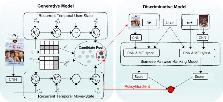
Figure 1. The Architecture of Long-term and Session-based Ranking Model with Adversarial Network.

3.1. Matrix Factorization (MF)

The MF framework (Mnih and Salakhutdinov, 2008) models the long-term states (global information) for both users ($\mathbf{e}^{u}$) and movies ($\mathbf{e}^{m}$). In its standard setting, the recommendation task can be formulated as inferring missing values of a partially observed user-movie rating matrix $R$. The formulation of MF is given by:

(1) $$\operatorname*{argmin}_{\mathbf{e}^{u},\mathbf{e}^{m}}\sum_{i,j}I_{ij}\left(r_{ij}-\rho\left((\mathbf{e}^{u}_{i})^{T}\mathbf{e}^{m}_{j}\right)\right)^{2}+{\lambda^{u}}\|\mathbf{e}^{u}\|_{F}^{2}+{\lambda^{m}}\|\mathbf{e}^{m}\|_{F}^{2}$$

where $\mathbf{e}^{u}_{i}$ and $\mathbf{e}^{m}_{j}$ represent the user and movie latent factors in the shared $d$-dimension space respectively. $r_{ij}$ denotes the user $i$’s rating on movie $j$. $I_{ij}$ is an indicator function and equals 1 if $r_{ij}>0$, and 0 otherwise. $\lambda^{u}$ and $\lambda^{m}$ are regularization coefficients. The $\rho(\cdot)$ is a logistic scoring function that bounds the range of outputs.

In most recommender systems, matrix factorization techniques (Koren et al., 2009) recommend movies based on estimated ratings. Even though the predicted ratings can be used to rank the movies, it is known that it does not provide the best prediction for the top-$n$ recommendation. Because minimizing the objective function – the squared errors – does not perfectly align with the goal to optimize the ranking order. In this paper, we apply MF for ranking prediction (top-$n$ recommendation) directly, similar to (Wang et al., 2017).

3.2. Recurrent Neural Network (RNN)

The RNN based recommender system focuses on modeling session-based trajectories instead of global (long-term) information (Wu et al., 2017). It predicts future behaviors and provides users with a ranking list given the users’ past history. The main purpose of using RNN is to capture time-varying state for both users and movies. Particularly, we use LSTM cell as the basic RNN unit. Each LSTM unit at time $t$ consists of a memory cell $c_{t}$, an input gate $i_{t}$, a forget gate $f_{t}$, and an output gate $o_{t}$. These gates are computed from previous hidden state $\mathbf{h}_{t-1}$ and the current input $\mathbf{x}_{t}$:

(2) $$\left[f_{t},i_{t},o_{t}\right] =\text{sigmoid}(W[\mathbf{h}_{t-1},\mathbf{x}_{t}])$$

The memory cell $c_{t}$ is updated by partially forgetting the existing memory and adding a new memory content $\mathbf{l}_{t}$:

(3) $$\mathbf{l}_{t} =\tanh(V[\mathbf{h}_{t-1},\mathbf{x}_{t}])$$

(4) $$\mathbf{c}_{t} =f_{t}\odot\mathbf{c}_{t-1}+i_{t}\odot\mathbf{l}_{t}$$

Once the memory content of the LSTM unit is updated, the hidden state at time step $t$ is given by:

(5) $$\mathbf{h}_{t} =o_{t}\odot\tanh(\mathbf{c}_{t})$$

For simplicity of notation, the update of the hidden states of LSTM at time step $t$ is denoted as $\mathbf{h}_{t}={\rm LSTM}(\mathbf{h}_{t-1},\mathbf{x}_{t})$.

Here, we use $\mathbf{z}^{u}_{i,t}\in\mathbb{R}^{U}$ and $\mathbf{z}^{m}_{j,t}\in\mathbb{R}^{M}$ to represent the rating vector of user $i$ and movie $j$ given time $t$ respectively. Both $\mathbf{z}^{u}_{i,t}$ and $\mathbf{z}^{m}_{j,t}$ serve as the input to the LSTM layer at time $t$ to infer the new states of the user and the movie:

(6) $$\mathbf{h}^{u}_{i,t} ={\rm LSTM}(\mathbf{h}^{u}_{i,t-1},\mathbf{z}^{u}_{i,t})$$

(7) $$\mathbf{h}^{m}_{j,t} ={\rm LSTM}(\mathbf{h}^{m}_{j,t-1},\mathbf{z}^{m}_{j,t})$$

Here, $\mathbf{h}^{u}_{i,t}$ and $\mathbf{h}^{m}_{j,t}$ denote hidden states for user $i$ and movie $j$ at time step $t$ respectively.

In this work, we explore the potential of integrating posters of movies to boost the performance of movie recommendation. Inspired by the recent advances of CNNs in computer vision, the poster is mapped to the same space of the movie by using a CNN. More concretely, we encode each image into a FC-2k feature vector with Resnet-101 (101 layers), resulting in a 2048-dimensional vector representation. The poster $P_{j}$ of movie $j$ is only inputted once, at $t=0$, to inform the movie LSTM about the poster content:

(8) $$\mathbf{z}^{m}_{j,0}=CNN(P_{j}).$$

3.3. RNN and MF Hybrid

The session-based model deals with temporal dynamics of the user and movie states, we further incorporate the long-term preference of users and the fixed properties of movies. To exploit their advantages together, similar to (Wu et al., 2017), we define the rating prediction function as:

(9) $$r_{ij,t} =g(\mathbf{e}^{u}_{i},\mathbf{e}^{m}_{j},\mathbf{h}^{u}_{i,t},\mathbf{h}^{m}_{j,t})$$

where $g(.)$ is a score function, $\mathbf{e}^{u}_{i}$ and $\mathbf{e}^{m}_{j}$ denote the global latent factors of user $i$ and movie $j$ learned by Eq.  (1); $\mathbf{h}^{u}_{i,t}$ and $\mathbf{h}^{m}_{j,t}$ denote the hidden states at time step $t$ of two RNNs learned by Eq. (6) and Eq. (7) respectively. In this work, we study four strategies to calculate the score function $g$, integrating MF and RNN. The details are described below.

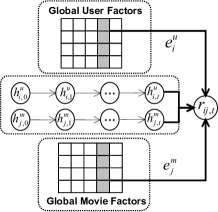
(a) LSIC-V1: Hard mechanism

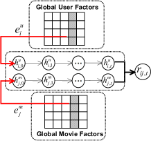
(b) LSIC-V2: Prior initialization

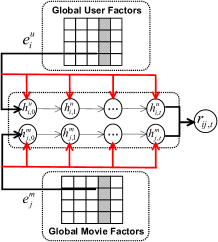
(c) LSIC-V3: Static context

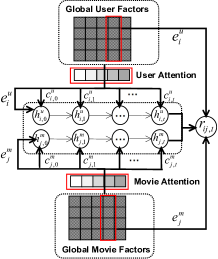
(d) LSIC-V4: Attention model

Figure 2. Four strategies to calculate the score function $g$, integrating MF and RNN.

LSIC-V1

This is a hard mechanism, using a simple way to calculate the mixing score from MF and RNN with the following formulation:

(10) $$r_{ij,t} =g(\mathbf{e}^{u}_{i},\mathbf{e}^{m}_{j},\mathbf{h}^{u}_{i,t},\mathbf{h}^{m}_{j,t})=\frac{1}{1+{\rm exp}(-\mathbf{s})}$$

(11) $$\mathbf{s} =\mathbf{e}^{u}_{i}\cdot\mathbf{e}^{m}_{j}+\mathbf{h}^{u}_{i,t}\cdot\mathbf{h}^{m}_{j,t}+b^{u}_{i}+b^{m}_{j}$$

where $b^{u}_{i}$ and $b^{m}_{j}$ are the biases of user $i$ and movie $j$; $\mathbf{h}^{u}_{i,t}$ and $\mathbf{h}^{m}_{j,t}$ are computed by Eq. (6) and Eq. (7).

In fact, LSIC-V1 does not exploit the global factors in learning the temporal dynamics. In this paper, we also design a soft mixture mechanism and provide three strategies to account for the global factors $\mathbf{e}^{u}_{i}$ and $\mathbf{e}^{m}_{j}$ in learning $\mathbf{h}^{u}_{i,t}$ and $\mathbf{h}^{m}_{j,t}$, as described below (i.e., LSIC-V2, LSIC-V3 and LSIC-V4).

LSIC-V2

We use the latent factors of user $i$ ($\mathbf{e}^{u}_{i}$) and movie $j$ ($\mathbf{e}^{m}_{j}$) pre-trained by MF model to initialize the hidden states of the LSTM cells $\mathbf{h}^{u}_{i,0}$ and $\mathbf{h}^{m}_{j,0}$ respectively, as depicted in Figure 2(b).

LSIC-V3

As shown in Figure 2(c), we extend LSIC-V2 by treating $\mathbf{e}^{u}_{i}$ (for user $i$) and $\mathbf{e}^{m}_{j}$ (for movie $j$) as the static context vectors, and feed them as an extra input into the computation of the temporal hidden states of users and movies by LSTM. At each time step, the context information assists the inference of the hidden states of LSTM model.

LSIC-V4

This method use an attention mechanism to compute a weight for each hidden state by exploiting the global factors. The mixing scores at time $t$ can be reformulated by:

(12) $$r_{ij,t} =g(\mathbf{e}^{u}_{i},\mathbf{e}^{m}_{j},\mathbf{h}^{u}_{i,t-1},\mathbf{h}^{m}_{j,t-1},\mathbf{c}^{u}_{i,t},\mathbf{c}^{m}_{j,t})=\frac{1}{1+{\rm exp}(-\mathbf{s})}$$

(13) $$\mathbf{s} =\mathbf{e}^{u}_{i}\cdot\mathbf{e}^{m}_{j}+\mathbf{h}^{u}_{i,t}\cdot\mathbf{h}^{m}_{j,t}+b_{i}+b_{j}$$

where $\mathbf{c}^{u}_{i,t}$ and $\mathbf{c}^{m}_{j,t}$ are the context vectors at time step $t$ for user $i$ and movie $j$; $\mathbf{h}^{u}_{i,t}$ and $\mathbf{h}^{m}_{j,t}$ are the hidden states of LSTMs at time step $t$, computed by

(14) $$\mathbf{h}^{u}_{i,t} ={\rm LSTM}(\mathbf{h}^{u}_{i,t-1},\mathbf{z}^{u}_{i,t},\mathbf{c}^{u}_{i,t})$$

(15) $$\mathbf{h}^{m}_{j,t} ={\rm LSTM}(\mathbf{h}^{m}_{j,t-1},\mathbf{z}^{m}_{j,t},\mathbf{c}^{m}_{j,t})$$

The context vectors $\mathbf{c}^{u}_{i,t}$ and $\mathbf{c}^{m}_{j,t}$ act as extra input in the computation of the hidden states in LSTMs to make sure that every time step of the LSTMs can get full information of the context (long-term information). The context vectors $\mathbf{c}^{u}_{i,t}$ and $\mathbf{c}^{m}_{j,t}$ are the dynamic representations of the relevant long-term information for user $i$ and movie $j$ at time $t$, calculated by

(16) $$\mathbf{c}^{u}_{i,t}=\sum_{k=1}^{U}\alpha^{i}_{k,t}\mathbf{e}^{u}_{k};\hskip 8.5359pt\mathbf{c}^{m}_{j,t}=\sum_{p=1}^{M}\beta^{j}_{p,t}\mathbf{e}^{m}_{p}$$

where $U$ and $M$ are the number of users and movies. The attention weights $\alpha^{i}_{k,t}$ and $\beta^{j}_{p,t}$ for user $i$ and movie $j$ at time step $t$ are computed by

(17) $$\alpha^{i}_{k,t}=\frac{\exp(\sigma(\mathbf{h}^{u}_{i,t-1},\mathbf{e}^{u}_{k}))}{\sum_{k^{\prime}=1}^{U}\exp(\sigma(\mathbf{h}^{u}_{i,t-1},\mathbf{e}^{u}_{k^{\prime}}))}$$

(18) $$\beta^{j}_{p,t}=\frac{\exp(\sigma(\mathbf{h}^{m}_{j,t-1},\mathbf{e}^{m}_{p}))}{\sum_{p^{\prime}=1}^{M}\exp(\sigma(\mathbf{h}^{m}_{j,t-1},\mathbf{e}^{m}_{p^{\prime}}))}$$

where $\sigma$ is a feed-forward neural network to produce a real-valued score. The attention weights $\alpha^{i}_{t}$ and $\beta^{j}_{t}$ together determine which user and movie factors should be selected to generate $r_{ij,t}$.

3.4. Generative Adversarial Network (GAN) for Recommendation

Generative adversarial network (GAN)(Goodfellow et al., 2014) consist of a generator G and a discriminator D that compete in a minimax game with two players: The discriminator tries to distinguish real high-rated movies on training data from ranking or recommendation list predicted by G, and the generator tries to fool the discriminator to generate(predict) well-ranked recommendation list. Concretely, D and G play the following game on V(D,G):

(19) $$\min_{G}\max_{D}v(D,G)= \mathbb{E}_{x\sim P_{true}(x)}[{\rm log}D(x)]+$$

$$\mathbb{E}_{z\sim P_{z}(z)}[{\rm log}(1-D(G(z)))]$$

Here, $x$ is the input data from training set, $z$ is the noise variable sampled from normal distribution.

We propose an adversarial framework to iteratively optimize two models: the generative model $G$ predicting recommendation list given historical user-movie interactions, and the discriminative model $D$ predicting the relevance of the generated list. Like the standard generative adversarial networks (GANs) (Goodfellow et al., 2014), our model also optimizes the two models with a minimax two-player game. $D$ tries to distinguish the real high-rated movies in the training data from the recommendation list generated by $G$, while $G$ maximizes the probability of $D$ making a mistake. Hopefully, this adversarial process can eventually adjust $G$ to generate plausible and high-quality recommendation list. We further elaborate the generator and discriminator below.

3.4.1. Discriminate Model

As depicted in Figure 1 (right side), we implement the discriminator $D$ via a Siamese Network that incorporates long and session-based ranking models in a pair-wise scenario. The discriminator $D$ has two symmetrical point-wise networks that share parameters and are updated by minimizing a pair-wise loss.

The objective of discriminator $D$ is to maximize the probability of correctly distinguishing the ground truth movies from generated recommendation movies. For $G$ fixed, we can obtain the optimal parameters for the discriminator $D$ with the following formulation.

(20) $$\theta^{*}=\operatorname*{argmax}_{\theta}\sum_{i\in\mathcal{U}}\Big{(}\mathbb{E}_{m_{+},m_{-}\sim p_{true}}\left[{\log}D_{\theta}(u_{i},m_{-},m_{+}|t)\right]+$$

$$\mathbb{E}_{m_{+}\sim p_{true},m_{g,t}\sim G_{\phi}(m_{g,t}|u_{i},t)}\left[{\log}(1-D_{\theta}(u_{i},m_{g,t},m_{+}|t)\right]\Big{)}$$

where $\mathcal{U}$ denotes the user set, $u_{i}$ denotes user $i$, $m_{+}$ is a positive (high-rating) movie, $m_{-}$ is a negative movie randomly chosen from the entire negative (low-rating) movie space, $\theta$ and $\phi$ are parameters of $D$ and $G$, and $m_{g,t}$ is the generated movie by $G$ given time $t$. Here, we adopt hinge loss as our training objective since it performs better than other training objectives. Hinge loss is widely adopted in various learning to rank scenario, which aims to penalize the examples that violate the margin constraint:

(21) $$D(u_{i},m_{-},m_{+}|t)=\max\Big{\{}0,\epsilon-g(\mathbf{e}^{u}_{i},\mathbf{e}^{m}_{m_{+}},\mathbf{h}^{u}_{i,t},\mathbf{h}^{m}_{m_{+},t})$$

$$+g(\mathbf{e}^{u}_{i},\mathbf{e}^{m}_{m_{-}},\mathbf{h}^{u}_{i,t},\mathbf{h}^{m}_{m_{-},t})\Big{\}}$$

where $\epsilon$ is the hyper-parameter determining the margin of hinge loss, and we compress the outputs to the range of $(0,1)$.

3.4.2. Generative Model

Similar to conditional GANs proposed in (Mirza and Osindero, 2014), our generator $G$ takes in the auxiliary information (user $u_{i}$ and time $t$) as input, and generates the ranking list for user $i$. Specifically, when D is optimized and fixed after computing Eq. 20, the generator $G$ can be optimized by minimizing the following formulation:

(22) $$\phi^{*}=\operatorname*{argmin}_{\phi}\sum_{m\in\mathcal{M}}\big{(}\mathbb{E}_{m_{g,t}\sim G_{\phi}(m_{g,t}|u_{i},t)}[{\rm log}(1-D(u_{i},m_{g,t},m_{+}|t)]\big{)}$$

Here, $\mathcal{M}$ denotes the movie set. As in (Goodfellow et al., 2014), instead of minimizing ${\rm log}(1-D(u_{i},m_{g,t},m_{+}|t))$, we train $G$ to maximize ${\rm log}(D(u_{i},m_{g,t},m_{+}|t))$.

3.4.3. Policy Gradient

Since the sampling of recommendation list by generator $G$ is discrete, it cannot be directly optimized by gradient descent as in the standard GAN formulation. Therefore, we use policy gradient based reinforcement learning algorithm (Sutton et al., 2000) to optimize the generator $G$ so as to generate highly rewarded recommendation list. Concretely, we have the following derivations:

(23) $$\nabla_{\phi}J^{G}(u_{i}) =\nabla_{\phi}\mathbb{E}_{m_{g,t}\sim G_{\phi}(m_{g,t}|u_{i},t)}[\log D(u_{i},m_{g,t},m_{+}|t)]$$

$$=\sum_{m\in\mathcal{M}}\nabla_{\phi}G_{\phi}(m|u_{i},t)\log D(u_{i},m,m_{+}|t)$$

$$=\sum_{m\in\mathcal{M}}G_{\phi}(m|u_{i},t)\nabla_{\phi}\log G_{\phi}(m|u_{i},t)\log D(u_{i},m,m_{+}|t)$$

$$=\mathbb{E}_{m_{g,t}\sim G_{\phi}(m|u_{i},t)}[\nabla_{\phi}{\rm log}G_{\phi}(m_{g,t}|u_{i},t)\log D(u_{i},m_{g,t},m_{+}|t)]$$

$$\approx\frac{1}{K}\sum_{k=1}^{K}\nabla_{\phi}{\rm log}G_{\phi}(m_{k}|u_{i},t)\log D(u_{i},m_{k},m_{+}|t)$$

where $K$ is number of movies sampled by the current version of generator and $m_{k}$ is the $k$-th sampled item. With reinforcement learning terminology, we treat the term ${\rm log}D(u_{i},m_{k},m_{+}|t)$ as the reward at time step $t$, and take an action $m_{k}$ at each time step. To accelerate the convergence, the rewards within a batch are normalized with a Gaussian distribution to make the significant differences.

1 Input: generator $G_{\phi}$, discriminator $D_{\theta}$, training data $S$.

2 Initialize models $G_{\phi}$ and $D_{\theta}$ with random weights, and pre-train them on training data $S$.

3 repeat

4 for g-steps do

5       Generate recommendation list for user $i$ at time $t$ using the generator $G_{\phi}$.

6       Sample $K$ candidates from recommendation list.

7       for $k\in\{1,...,K\}$ do

8             Sample a positive movie $m_{+}$ from S.

9             Compute the reward ${\rm log}D(u_{i},m_{k},m_{+}|t)$ with Eq.(21)

10            

11      Update generator $G_{\phi}$ via policy gradient Eq.(23).

12      

13for d-steps do

14       Use current $G_{\phi}$ to generate a negative movie and combined with a positive movie sampled from $S$.

15       Update discriminator $D_{\theta}$ with Eq.(20).

16      

until convergence

Algorithm 1 Long and Session-based Ranking Model with Adversarial Network

The overall procedure is summarized in Algorithm 1. During the training stage, the discriminator and the generator are trained alternatively in a adversarial manner via Eq.(20) and Eq.(23), respectively.

4. Experimental Setup

4.1. Datasets

Table 2. Characteristics of the datasets.

Dataset	Movielens-100K	Netflix-3M	Netflix-Full
Users	943	326,668	480,189
movies	1,6831	17,751	17,770
Ratings	100,000	16,080,980	100,480,507
Train Data	09/97-03/98	9/05-11/05	12/99-11/05
Test Data	03/98-04/98	12/05	12/05
Train Ratings	77,714	13,675,402	98,074,901
Test Ratings	21,875	2,405,578	2,405,578
Density	0.493	0.406	0.093
Sparsity	0.063	0.003	0.012

In order to evaluate the effectiveness of our model, we conduct experiments on two widely-used real-life datasets: Movielens100K and Netflix (called “Netflix-Full”). To evaluate the robustness of our model, we also conduct experiments on a 3-month Netflix (called “Netflix-3M”) dataset, which is a small version of Netflix-Full and has different training and testing period. For each dataset, we split the whole data into several training and testing intervals based on time, as is done in (Wu et al., 2017), to simulate the actual situation of predicting future behaviors of users given the data that occurred strictly before current time step. Then, each testing interval is randomly divided into a validation set and a testing set. We removed the users and movies that do not appear in training set from the validation and test sets. The detailed statistics are presented in Table 2. Following (Wang et al., 2017), we treat “5-star” in Netflix, “4-start” and “5-start” for Movielens100K as positive feedback and all others as unknown (negative) feedback.

4.2. Implementation Details

Matrix Factorization.

We use matrix factorization with 5 and 16 factor numbers for Movielens and Netflix respectively (Wang et al., 2017). The parameters are randomly initialized by a uniform distribution ranged in [-0.05, 0.05]. We take gradient-clipping to suppress the gradient to the range of [-0.2,0.2]. L2 regularization (with $\lambda=0.05$) is used to the weights and biases of user and movie factors.

Recurrent Neural Network.

We use a single-layer LSTM with 10 hidden neurons, 15-dimensional input embeddings, and 4-dimensional dynamic states where each state contains 7-days users/movies behavioral trajectories. That is, we take one month as the length of a session. The parameters are initialized with the same way as in MF. L2 regularization (with $\lambda=0.05$) is used to the weights and biases of the LSTM layer to avoid over-fitting.

Generative Adversarial Nets.

We pre-train $G$ and $D$ on the training data with a pair-wise scenario, and use SGD algorithm with learning rate $1\times 10^{-4}$ to optimize its parameters. The number of sampled movies is set to 64 (i.e., $K=64$). In addition, we use matrix factorization model to generate 100 candidate movies, and then re-rank these movies with LSTM. In all experiments, we conduct mini-batch training with batch size 128.

4.3. Evaluation Metrics

To quantitatively evaluate our method, we adopt the rank-based evaluation metrics to measure the performance of top-$n$ recommendation (Liu and Yang, 2008; Cremonesi et al., 2010) , including Precision@N, Normalised Discounted Cumulative Gain (NDCG@N), Mean Average Precision (MAP) and Mean Reciprocal Ranking (MRR).

4.4. Comparison to Baselines

In the experiments, we evaluate and compare our models with several state-of-the-art methods.

Table 3. Moive recommendation results (MovieLens).

	Precision@3	Precision@5	Precision@10	NDCG@3	NDCG@5	NDCG@10	MRR	MAP
BPR	0.2795	0.2664	0.2301	0.2910	0.2761	0.2550	0.4324	0.3549
PRFM	0.2884	0.2699	0.2481	0.2937	0.2894	0.2676	0.4484	0.3885
LambdaFM	0.3108	0.2953	0.2612	0.3302	0.3117	0.2795	0.4611	0.4014
RRN	0.2893	0.2740	0.2480	0.2951	0.2814	0.2513	0.4320	0.3631
IRGAN	0.3022	0.2885	0.2582	0.3285	0.3032	0.2678	0.4515	0.3744
LSIC-V1	0.2946	0.2713	0.2471	0.2905	0.2801	0.2644	0.4595	0.4066
LSIC-V2	0.3004	0.2843	0.2567	0.3122	0.2951	0.2814	0.4624	0.4101
LSIC-V3	0.3105	0.3023	0.2610	0.3217	0.3086	0.2912	0.4732	0.4163
LSIC-V4	0.3327	0.3173	0.2847	0.3512	0.3331	0.2939	0.4832	0.4321
Impv	7.05%	7.45%	9.00%	6.36%	6.87%	5.15%	4.79%	7.65%

Table 4. Movie recommendation results (Netflix-3M).

	Precision@3	Precision@5	Precision@10	NDCG@3	NDCG@5	NDCG@10	MRR	MAP
BPR	0.2670	0.2548	0.2403	0.2653	0.2576	0.2469	0.3829	0.3484
PRFM	0.2562	0.2645	0.2661	0.2499	0.2575	0.2614	0.4022	0.3712
LambdaFM	0.3082	0.2984	0.2812	0.3011	0.2993	0.2849	0.4316	0.4043
RRN	0.2759	0.2741	0.2693	0.2685	0.2692	0.2676	0.3960	0.3831
IRGAN	0.2856	0.2836	0.2715	0.2824	0.2813	0.2695	0.4060	0.3718
LSIC-V1	0.2815	0.2801	0.2680	0.2833	0.2742	0.2696	0.4416	0.4025
LSIC-V2	0.2901	0.2883	0.2701	0.2903	0.2831	0.2759	0.4406	0.4102
LSIC-V3	0.3152	0.3013	0.2722	0.2927	0.2901	0.2821	0.4482	0.4185
LSIC-V4	0.3221	0.3193	0.2921	0.3157	0.3114	0.2975	0.4501	0.4247
Impv	4.51%	7.00%	3.88%	4.85%	4.04%	4.42%	4.29%	5.05%

Table 5. Movie recommendation results (Netflix-Full).

	Precision@3	Precision@5	Precision@10	NDCG@3	NDCG@5	NDCG@10	MRR	MAP
BPR	0.3011	0.2817	0.2587	0.2998	0.2870	0.2693	0.3840	0.3660
PRFM	0.2959	0.2837	0.2624	0.2831	0.2887	0.2789	0.4060	0.3916
LambdaFM	0.3446	0.3301	0.3226	0.3450	0.3398	0.3255	0.4356	0.4067
RRN	0.3135	0.2954	0.2699	0.3123	0.3004	0.2810	0.3953	0.3768
IRGAN	0.3320	0.3229	0.3056	0.3319	0.3260	0.3131	0.4248	0.4052
LSIC-V1	0.3127	0.3012	0.2818	0.3247	0.3098	0.2957	0.4470	0.4098
LSIC-V2	0.3393	0.3271	0.3172	0.3482	0.3401	0.3293	0.4448	0.4213
LSIC-V3	0.3501	0.3480	0.3291	0.3498	0.3451	0.3321	0.4503	0.4257
LSIC-V4	0.3621	0.3530	0.3341	0.3608	0.3511	0.3412	0.4587	0.4327
Impv	5.08%	6.94%	3.56%	4.58%	3.33%	4.82%	5.30%	6.39%

Table 6. Ablation results for Netflix-3M dataset.

	Precision@3	Precision@5	Precision@10	NDCG@3	NDCG@5	NDCG@10	MRR	MAP
LSIC-V4	0.3221	0.3193	0.2921	0.3157	0.3114	0.2975	0.4501	0.4247
w/o RL	0.3012	0.2970	0.2782	0.2988	0.2927	0.2728	0.4431	0.4112
w/o poster	0.3110	0.3012	0.2894	0.3015	0.3085	0.2817	0.4373	0.4005

Table 7. The Recalled movies from Top-10 candidates in Neflix-3M dataset

	Groundtruth	IRGAN (Wang et al., 2017)	RRN (Wu et al., 2017)	LambdaFM (Yuan et al., 2016)	LSIC-V4
Userid: 1382	9 Souls The Princess Bride Stuart Saves His Family The Last Valley Wax Mask After Hours Session 9 Valentin	[1] The Beatles: Love Me Do [2] Wax Mask ✓ [3] Stuart Saves His Family ✓ [4] After Hours ✓ [5] Top Secret! [6] Damn Yankees [7] Dragon Tales: It’s Cool to Be Me! [8] Play Misty for Me [9] The Last Round: Chuvalo vs. Ali’ [10] La Vie de Chateau	[1] Falling Down [2] 9 Souls ✓ [3] Wax Mask ✓ [4] After Hours ✓ [5] Stuart Saves His Family ✓ [6] Crocodile Dundee 2 [7] The Princess Bride ✓ [8] Dragon Tales: It’s Cool to Be Me! [9] They Were Expendable [10] Damn Yankees	[1] The Avengers ’63 [2] Wax Mask ✓ [3] The Boondock Saints [4] Valentin ✓ [5] 9 Souls ✓ [6] The Princess Bride ✓ [7] After Hours ✓ [8] Tekken [9] Stuart Saves His Family ✓ [10] Runn Ronnie Run	[1]9 Souls ✓ [2]The Princess Bride ✓ [3]Stuart Saves His Family ✓ [4] The Last Valley ✓ [5] Wax Mask ✓ [6] Session 9 ✓ [7] Dragon Tales: It’s Cool to Be Me! [8] Damn Yankees [9] After Hours ✓ [10] Valentin ✓
Userid: 8003	9 Souls Princess Bride	[1] Cheech Chong’s Up in Smoke [2] Wax Mask [3] Damn Yankees [4] Dragon Tales: It’s Cool to Be Me! [5] Top Secret! [6] Agent Cody Banks 2: Destination London [7] After Hours [8] Stuart Saves His Family [9] 9 Souls ✓ [10] The Beatles: Love Me Do	[1] Crocodile Dundee 2 [2] Session 9 [3] Falling Down [4] Wax Mask [5] After Hours [6] Stuart Saves His Family [7] 9 Souls ✓ [8] The Princess Bride ✓ [9] Dragon Tales: It’s Cool to Be Me! [10] Scream 2	[1] The Insider [2]A Nightmare on Elm Street 3 [3] Dennis the Menace Strikes Again [4] Civil Brand [5] 9 Souls ✓ [6] Falling Down [7] The Princess Bride ✓ [8] Radiohead: Meeting People [9] Crocodile Dundee 2 [10] Christmas in Connecticut	[1] 9 Souls ✓ [2]The Princess Bride ✓ [3]The Last Valley [4]Stuart Saves His Family [5]Wax Mask [6]Dragon Tales: It’s Cool to Be Me! [7]Session 9 [8]Crocodile Dundee 2 [9]Damn Yankees [10]Cheech Chong’s Up in Smoke

Bayesian Personalised Ranking (BPR)

Given a positive movie, BPR uniformly samples negative movies to resolve the imbalance issue and provides a basic baseline for top-N recommendation  (Rendle et al., 2009).

Pairwise Ranking Factorization Machine (PRFM)

This is one of the state-of-the-art movie recommendation algorithms, which applies Factorization Machine model to microblog ranking on basis of pairwise classification (Qiang et al., 2013). We use the same settings as in (Qiang et al., 2013) in our experiments.

LambdaFM

It is a strong baseline for recommendation, which directly optimizes the rank biased metrics (Yuan et al., 2016). We run the LambdaFM model with the publicly available code, and use default settings for all hyperparameters.

Recurrent Recommender Networks (RRN)

This model supplements matrix factorization with recurrent neural network model via a hard mixture mechanism (Wu et al., 2017). We use the same setting as in (Wu et al., 2017).

IRGAN

This model trains the generator and discriminator alternatively with MF in an adversarial process  (Wang et al., 2017). We run the IRGAN model with the publicly available code, and use default settings for all hyperparameters.

5. Experimental Results

In this section, we compare our model with baseline methods quantitatively and qualitatively.

5.1. Quantitative Evaluation

We first evaluate the performance of top-$n$ recommendation. The experimental results are summarized in Tables 3 ,4 and 5. Our model substantially and consistently outperforms the baseline methods by a noticeable margin on all the experimental datasets. In particular, we have explored several versions of our model with different mixture mechanisms. As one anticipates, LSIC-V4 achieves the best results across all evaluation metrics and all datasets. For example, on MovieLens dataset, LSIC-V4 improves $7.45\%$ on percision@5 and $6.87\%$ on NDCG@5 over the baseline methods. The main strength of our model comes from its capability of prioritizing both long-term and short-term information in content-aware movie recommendation. In addition, our mixture mechanisms (hard and soft) also seem quite effective to integrate MF and RNN.

To better understand the adversarial training process, we visualize the learning curves of LSIC-V4 as shown in Figure 3. Due to the limited space, we only report the Pecision@5 and NDCG@5 scores as in (Wang et al., 2017). The other metrics exhibit a similar trend. As shown in Figure 3, after about 50 epoches, both Precision@5 and NDCG@5 converge and the winner player is the generator which is used to generate recommendation list for our final top-$n$ movie recommendation. The performance of generator $G$ becomes better with the effective feedback (reward) from discriminator $D$. On the other hand, once we have a set of high-quality recommendation movies, the performance of $D$ deteriorates gradually in the training procedure and makes mistakes for predictions. In our experiments, we use the generator G with best performance to predict test data.

5.2. Ablation Study

In order to analyze the effectiveness of different components of our model for top-$n$ movie recommendation, in this section, we report the ablation test of LSIC-V4 by discarding poster information (w/o poster) and replacing the reinforcement learning with Gumbel-Softmax (Kusner and Hernández-Lobato, 2016) (w/o RL), respectively. Gumbel-Softmax is an alternative method to address the non-differentiation problem so that $G$ can be trained straightforwardly.

Due to the limited space, we only illustrate the experimental results for Netflix-3M dataset that is widely used in movie recommendation (see Table 6). Generally, both factors contribute, and reinforcement learning contributes most. This is within our expectation since discarding reinforcement learning will lead the adversarial learning inefficient. With Gumbel-Softmax, $G$ does not benefit from the reward of $D$, so that we do not know which movies sampled by G are good and should be reproduced. Not surprisingly, poster information also contributes to movie recommendation.

5.3. Case Study

In this section, we will further show the advantages of our models through some quintessential examples.

In Table 7, we provide the recommendation lists generated by three state-of-the-art baseline methods (i.e., IRGAN, RNN, LambdaFM) as well as the proposed LSIC-V4 model for two users who are randomly selected from the Netflix-3M dataset. Our model can rank the positive movies in higher positions than other methods. For example, the ranking of the movie “9 souls” for user “8003” has increased from 5-th position (by LambdaFM) to 1st position (by LSIC-V4). Meanwhile some emerging movies such as “Session 9” and “The Last Valley” that are truly attractive to the user “1382” have been recommended by our models, whereas they are ignored by baseline methods. In fact, we can include all positive movies in the top-10 list for user “1382” and in top-3 list for user “8003”. Our model benefits from the fact that both dynamic and static knowledge are incorporated into the model with adversarial training.

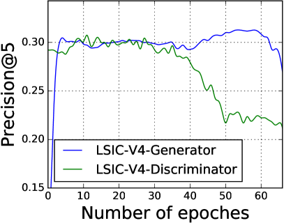
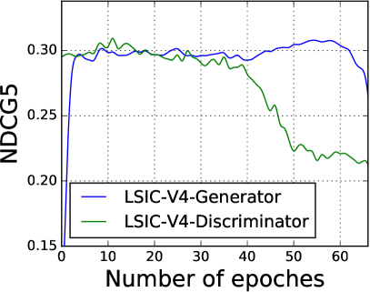
Figure 3. Learning curves of GAN on Netflix-3M

5.4. Re-rank Effect

From our experiments, we observe that it could be time-consuming for RNN to infer all movies. In addition, users may be interested in a few movies that are subject to a long-tailed distribution. Motivated by these observations, we provide a re-ranking strategy as used in (Covington et al., 2016). Specifically, we first generate $N$ candidate movies by MF, and then re-rank these candidate movies with our model. In this way, the inference time can been greatly reduced. Figure 4 illustrates the performance curves over the number of candidate movies (i.e. $N$) generated by MF. We only report the Pecision@5 and NDCG@5 results due to the limited space, the other metrics exhibit a similar trend. As shown in Figure 4, when the number of candidate movies is small, i.e., $N\leq 100$ for Netflix-3M dataset, the Percision@5 raises gradually with the number of candidate movies increases. Nevertheless, the performance drops rapidly with the increasing candidate movies when $N\geq 100$. It suggests that the candidates in a long-tail side generated by MF is inaccurate and these candidate movies deteriorate the overall performance of the re-rank strategy.

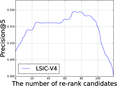
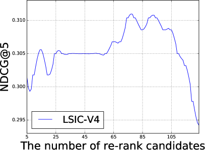
Figure 4. Sensitivity of the candidate scale on Netflix-3M

5.5. Session Period Sensitivity

The above experimental results have shown that the session-based (short-term) information indeed improves the performance of top-N recommendation. We conduct an experiment on Netflix-3M to investigate how the session period influences the final recommendation performance. As shown in Figure 5, the bars in purple color (below) describe the basic performance of MF component while the red ones (above) represent the extra improvement by the LSIC-V4. The RNN plays an insignificant role in the very early sessions since it lacks enough historical interaction data. For later period of sessions, RNN component tends to be more effective, and our joint model achieves a clear improvement over the model with only MF component.

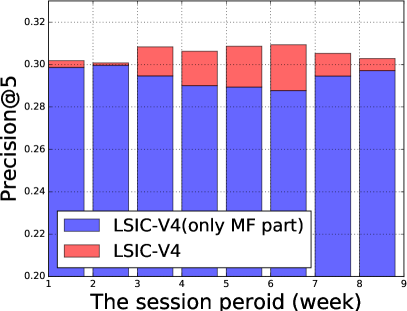
Figure 5. Sensitivity of the session period on Netflix-3M

6. Conclusion

In this paper, we proposed a novel adversarial process for top-$n$ recommendation. Our model incorporated both matrix factorization and recurrent neural network to exploit the benefits of the long-term and short-term knowledge. We also integrated poster information to further improve the performance of movie recommendation. Experiments on two real-life datasets showed the performance superiority of our model.

References

- (1)
- Adomavicius and Tuzhilin (2005) Gediminas Adomavicius and Alexander Tuzhilin. 2005. Toward the next generation of recommender systems: A survey of the state-of-the-art and possible extensions. IEEE transactions on knowledge and data engineering 17, 6 (2005), 734–749.
- Arjovsky et al. (2017) Martin Arjovsky, Soumith Chintala, and Léon Bottou. 2017. Wasserstein generative adversarial networks. In International Conference on Machine Learning. 214–223.
- Bobadilla et al. (2013) Jesus Bobadilla, Fernando Ortega, Antonio Hernando, and Abraham Gutierrez. 2013. Recommender systems survey. Knowledge-based systems 46 (2013), 109–132.
- Chen et al. (2017) Tseng-Hung Chen, Yuan-Hong Liao, Ching-Yao Chuang, Wan-Ting Hsu, Jianlong Fu, and Min Sun. 2017. Show, Adapt and Tell: Adversarial Training of Cross-domain Image Captioner. arXiv preprint arXiv:1705.00930 (2017).
- Covington et al. (2016) Paul Covington, Jay Adams, and Emre Sargin. 2016. Deep neural networks for youtube recommendations. In Proceedings of the 10th ACM Conference on Recommender Systems. ACM, 191–198.
- Cremonesi et al. (2010) Paolo Cremonesi, Yehuda Koren, and Roberto Turrin. 2010. Performance of recommender algorithms on top-n recommendation tasks. In Proceedings of the fourth ACM conference on Recommender systems. ACM, 39–46.
- Cui et al. (2016) Qiang Cui, Shu Wu, Qiang Liu, and Liang Wang. 2016. A Visual and Textual Recurrent Neural Network for Sequential Prediction. arXiv preprint arXiv:1611.06668 (2016).
- Devooght and Bersini (2016) Robin Devooght and Hugues Bersini. 2016. Collaborative filtering with recurrent neural networks. arXiv preprint arXiv:1608.07400 (2016).
- Goodfellow et al. (2014) Ian Goodfellow, Jean Pouget-Abadie, Mehdi Mirza, Bing Xu, David Warde-Farley, Sherjil Ozair, Aaron Courville, and Yoshua Bengio. 2014. Generative adversarial nets. In Advances in neural information processing systems. 2672–2680.
- He et al. (2016) Xiangnan He, Hanwang Zhang, Min-Yen Kan, and Tat-Seng Chua. 2016. Fast matrix factorization for online recommendation with implicit feedback. In Proceedings of the 39th International ACM SIGIR conference on Research and Development in Information Retrieval. ACM, 549–558.
- Hernando et al. (2016) Antonio Hernando, Jesús Bobadilla, and Fernando Ortega. 2016. A non negative matrix factorization for collaborative filtering recommender systems based on a Bayesian probabilistic model. Knowledge-Based Systems 97 (2016), 188–202.
- Hidasi et al. (2015) Balázs Hidasi, Alexandros Karatzoglou, Linas Baltrunas, and Domonkos Tikk. 2015. Session-based recommendations with recurrent neural networks. In ICLR.
- Hochreiter and Schmidhuber (1997) Sepp Hochreiter and Jürgen Schmidhuber. 1997. Long short-term memory. Neural computation 9, 8 (1997), 1735–1780.
- Koren (2008) Yehuda Koren. 2008. Factorization meets the neighborhood: a multifaceted collaborative filtering model. In Proceedings of the 14th ACM SIGKDD international conference on Knowledge discovery and data mining. ACM, 426–434.
- Koren (2010) Yehuda Koren. 2010. Collaborative filtering with temporal dynamics. Commun. ACM 53, 4 (2010), 89–97.
- Koren et al. (2009) Yehuda Koren, Robert Bell, and Chris Volinsky. 2009. Matrix factorization techniques for recommender systems. Computer 42, 8 (2009).
- Kusner and Hernández-Lobato (2016) Matt J Kusner and José Miguel Hernández-Lobato. 2016. GANS for Sequences of Discrete Elements with the Gumbel-softmax Distribution. arXiv preprint arXiv:1611.04051 (2016).
- Liu and Yang (2008) Nathan N Liu and Qiang Yang. 2008. Eigenrank: a ranking-oriented approach to collaborative filtering. In Proceedings of the 31st annual international ACM SIGIR conference on Research and development in information retrieval. ACM, 83–90.
- Lu et al. (2015) Jie Lu, Dianshuang Wu, Mingsong Mao, Wei Wang, and Guangquan Zhang. 2015. Recommender system application developments: a survey. Decision Support Systems 74 (2015), 12–32.
- McNee et al. (2006) Sean M McNee, John Riedl, and Joseph A Konstan. 2006. Being accurate is not enough: how accuracy metrics have hurt recommender systems. In CHI’06 extended abstracts on Human factors in computing systems. ACM, 1097–1101.
- Mirza and Osindero (2014) Mehdi Mirza and Simon Osindero. 2014. Conditional generative adversarial nets. arXiv preprint arXiv:1411.1784 (2014).
- Mnih and Salakhutdinov (2008) Andriy Mnih and Ruslan R Salakhutdinov. 2008. Probabilistic matrix factorization. In Advances in neural information processing systems. 1257–1264.
- Qiang et al. (2013) Runwei Qiang, Feng Liang, and Jianwu Yang. 2013. Exploiting ranking factorization machines for microblog retrieval. In Proceedings of the 22nd ACM international conference on Conference on information & knowledge management. ACM, 1783–1788.
- Reed et al. (2016) Scott Reed, Zeynep Akata, Xinchen Yan, Lajanugen Logeswaran, Bernt Schiele, and Honglak Lee. 2016. Generative adversarial text to image synthesis. In Proceedings of the 33rd International Conference on International Conference on Machine Learning. JMLR.org, 1060–1069.
- Rendle et al. (2009) Steffen Rendle, Christoph Freudenthaler, Zeno Gantner, and Lars Schmidt-Thieme. 2009. BPR: Bayesian personalized ranking from implicit feedback. In Proceedings of the twenty-fifth conference on uncertainty in artificial intelligence. AUAI Press, 452–461.
- Rennie and Srebro (2005) Jasson DM Rennie and Nathan Srebro. 2005. Fast maximum margin matrix factorization for collaborative prediction. In Proceedings of the 22nd international conference on Machine learning. ACM, 713–719.
- Srebro et al. (2005) Nathan Srebro, Jason Rennie, and Tommi S Jaakkola. 2005. Maximum-margin matrix factorization. In Advances in neural information processing systems. 1329–1336.
- Sutton et al. (2000) Richard S Sutton, David A McAllester, Satinder P Singh, and Yishay Mansour. 2000. Policy gradient methods for reinforcement learning with function approximation. In Advances in neural information processing systems. 1057–1063.
- Wang et al. (2017) Jun Wang, Lantao Yu, Weinan Zhang, Yu Gong, Yinghui Xu, Benyou Wang, Peng Zhang, and Dell Zhang. 2017. IRGAN: A Minimax Game for Unifying Generative and Discriminative Information Retrieval Models. In Proceedings of the 40th International ACM SIGIR Conference on Research and Development in Information Retrieval. 515–524.
- Wu et al. (2016) Caihua Wu, Junwei Wang, Juntao Liu, and Wenyu Liu. 2016. Recurrent neural network based recommendation for time heterogeneous feedback. Knowledge-Based Systems 109 (2016), 90–103.
- Wu et al. (2016) Chao-Yuan Wu, Amr Ahmed, Alex Beutel, and Alexander J Smola. 2016. Joint Training of Ratings and Reviews with Recurrent Recommender Networks. ICLR (2016).
- Wu et al. (2017) Chao-Yuan Wu, Amr Ahmed, Alex Beutel, Alexander J Smola, and How Jing. 2017. Recurrent recommender networks. In Proceedings of the Tenth ACM International Conference on Web Search and Data Mining. ACM, 495–503.
- Yu et al. (2017) Lantao Yu, Weinan Zhang, Jun Wang, and Yong Yu. 2017. SeqGAN: Sequence Generative Adversarial Nets with Policy Gradient.. In AAAI. 2852–2858.
- Yuan et al. (2016) Fajie Yuan, Guibing Guo, Joemon M Jose, Long Chen, Haitao Yu, and Weinan Zhang. 2016. Lambdafm: learning optimal ranking with factorization machines using lambda surrogates. In Proceedings of the 25th ACM International on Conference on Information and Knowledge Management. ACM, 227–236.
- Zhao et al. (2016) Lili Zhao, Zhongqi Lu, Sinno Jialin Pan, and Qiang Yang. 2016. Matrix Factorization+ for Movie Recommendation.. In IJCAI. 3945–3951.