Time-dependent optimized coupled-cluster method for multielectron dynamics

Abstract

Time-dependent coupled-cluster method with time-varying orbital functions, called time-dependent optimized coupled-cluster (TD-OCC) method, is formulated for multielectron dynamics in an intense laser field. We have successfully derived equations of motion for CC amplitudes and orthonormal orbital functions based on the real action functional, and implemented the method including double excitations (TD-OCCD) and double and triple excitations (TD-OCCDT) within the optimized active orbitals. The present method is size extensive and gauge invariant, a polynomial cost-scaling alternative to the time-dependent multiconfiguration self-consistent-field method. The first application of the TD-OCC method to intense-laser driven correlated electron dynamics in Ar atom is reported.

introduction

The strong-field physics and ultrafast science are rapidly progressing towards a world-changing goal to directly measure and control the electron motion in matters.Protopapas, Keitel, and Knight (1997); Agostini and DiMauro (2004); Krausz and Ivanov (2009); Gallmann, Cirelli, and Keller (2013); Nisoli et al. (2017) Reliable theoretical and computational methods are indispensable to understand and predict strong-field and ultrafast phenomena, which frequently involve both bound excitations and ionizations, where dynamical electron correlation plays a key role.

One of the most advanced methods to describe such electron dynamics is the multiconfiguration time-dependent Hartree-Fock (MCTDHF) method,Zanghellini et al. (2003); Kato and Kono (2004); Caillat et al. (2005); Nest, Klamroth, and Saalfrank (2005) and more generally the time-dependent multiconfiguration self-consistent-field (TD-MCSCF) method.Nguyen-Dang et al. (2007); Ishikawa and Sato (2015) In TD-MCSCF, the electronic wavefunction is given by the configuration-interaction (CI) expansion, $\Psi_{\rm CI}(t)=\sum_{\bf I}C_{\bf I}(t)\Phi_{\bf I}(t)$, and both CI coefficiets $\{C_{\bf I}(t)\}$ and occupied spin-orbital functions $\{\psi_{p}(t)\}$ constituting the Slater determinants $\{\Phi_{\bf I}(t)\}$ are propagated in time. (Hereafter spin-orbital functions are simply referred to as orbitals. See, e.g, Refs. 12; 13; 14; 15 for TDCI methods using fixed orbitals, and Ref. 11 for a broad review of ab initio wavefunction-based methods for multielectron dynamics.) Though powerful, the full CI-based MCTDHF method suffers from the factorial scaling of the computational cost with respect to the number of electrons, which restricts its applicability to the systems of moderate size.

The time-dependent complete-active-space self-consistent-field (TD-CASSCF) methodSato and Ishikawa (2013) significantly reduces the cost by flexibly classifying occupied orbitals into frozen-core, dynamical-core, and active orbitals as defined in Fig. 1. More approximate and thus less demanding models have been actively investigated, Miyagi and Madsen (2013, 2014); Haxton and McCurdy (2015); Sato and Ishikawa (2015) which rely on the truncaed CI expansion within the active orbitals given, e.g, as

$$\Psi_{\rm CI}=(C_{0}+C^{a}_{i}\hat{E}^{a}_{i}+C^{ab}_{ij}\hat{E}^{ab}_{ij}+C^{abc}_{ijk}\hat{E}^{abc}_{ijk}+\cdots)\Phi,$$ (1)

where (Einstein’s summation convention is implied throughout for orbital indices.) $\hat{E}^{abc\cdots}_{ijk\cdots}=\hat{c}^{\dagger}_{a}\hat{c}^{\dagger}_{b}\hat{c}^{\dagger}_{c}\cdots\hat{c}_{k}\hat{c}_{j}\hat{c}_{i}$ [$c^{\dagger}_{\mu}$ ($c_{\mu}$) is a creation (anihilation) operator for $\psi_{\mu}$] excites electron(s) from orbital(s) $i,j,k\cdots$ occupied in the reference determinant $\Phi$ (hole) to those $a,b,c\cdots$ not occupied in the reference (particle), achieving a polynomial cost scaling. Even though state-of-the-art real-space implementationsKato and Kono (2008); Hochstuhl and Bonitz (2011); Haxton, Lawler, and McCurdy (2012); Haxton and McCurdy (2014, 2015); Sato and Ishikawa (2016); Sawada, Sato, and Ishikawa (2016); Omiste, Li, and Madsen (2017); Orimo et al. have proved a great utility of these methods, all the methods based on a truncated-CI expansion share a common drawback of not being size extensive.Szabo and Ostlund (1996); Helgaker, Jørgensen, and Olsen (2002)

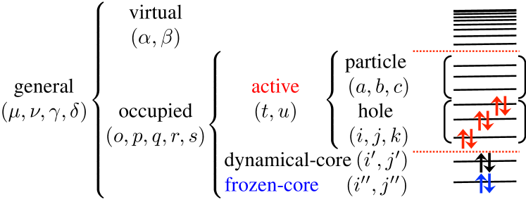
Figure 1: Illustration of the orbital subspacing (for a spin-degenerate case). The up and down arrows represent electrons, and horizontal lines represent spatial orbitals, classified into frozen-core (doubly occupied and fixed in time) and dynamical-core (doubly occupied but propagated in time) orbitals and active orbitals (correlated and propagated). The active orbital space is further splitted into the hole and particle subspaces. The index convention for orbitals of each group is given in the parentheses.

Therefore one naturally seeks an alternative to Eq. (1), where the truncated CI is replaced with the size-extensize coupled-cluster (CC) expansionSzabo and Ostlund (1996); Helgaker, Jørgensen, and Olsen (2002); Kümmel (2003); Shavitt and Bartlett (2009)

$$\Psi_{\rm CC}=\exp(\tau^{a}_{i}\hat{E}^{a}_{i}+\tau^{ab}_{ij}\hat{E}^{ab}_{ij}+\tau^{abc}_{ijk}\hat{E}^{abc}_{ijk}+\cdots)\Phi,$$ (2)

where both excitation amplitudes $\{\tau^{abc\cdots}_{ijk\cdots}(t)\}$ and orbitals are propagated in time, just as the stationary orbital-optimized CC (OCC) methodG. E. Scuseria and H. F. Schaefer III (1987); Sherrill et al. (1998); Krylov et al. (1998); Köhn and Olsen (2005) optimizes both excitation amplitudes and orbitals to minimize the CC energy functional. This idea was recently put forward by KvaalKvaal (2012), who, based on Arponen’s seminal work,Arponen (1983) developed a time-dependent coupled-cluster method using time-varying biorthonormal orbitals, called orbital-adapted time-dependent coupled-cluster (OATDCC) method, and applied it to the collision problem in a one-dimensional model Hamiltonian. This method, however, has a difficulty in obtaining the ground state of the system, required as an initial state of simulations, and has not yet been applied to real three-dimensional or time-dependent Hamiltonian. We also notice recent investigations on the time-dependent coupled-cluster methods using fixed orbitals.Huber and Klamroth (2011); D. R. Nascimento and A. E. DePrince III (2016) Their primary focus, however, has been placed on retrieving spectral information rather than the time-domain electron dynamics itself.

In this communication we report our successful formulation and implementation of the time-dependent coupled-cluster method using time-varying orthonormal orbitals, called time-dependent optimized coupled-cluster (TD-OCC) method, and present its first application to electron dynamics of Ar atom subject to an intense laser field. The Hartree atomic units are used throughout unless otherwise noted.

Time-dependent variational principle with real CC action functional

We are interested in the dynamics of a many-electron system interacting with external electromagnetic fields governed by the Hamiltonian written in the second quantization as

$$\quad\quad\quad\quad\hat{H}(t)=h^{\mu}_{\nu}(t)\hat{E}^{\mu}_{\nu}+\frac{1}{2}g^{\mu\gamma}_{\nu\delta}\hat{E}^{\mu\gamma}_{\nu\delta},$$ (3)

$$\quad\quad\quad h^{\mu}_{\nu}(t)=\int dx\psi^{*}_{\mu}[h_{0}+V_{\rm ext}(t)]\psi_{\nu},$$ (4)

$$g^{\mu\gamma}_{\nu\delta}=\int\int dx_{1}dx_{2}\psi^{*}_{\mu}(x_{1})\psi^{*}_{\gamma}(x_{2})r^{-1}_{12}\psi_{\nu}(x_{1})\psi_{\delta}(x_{2}),$$ (5)

where [$x\!=\!(\boldsymbol{r},\sigma)$ labels spatial-spin coordinate.] $h_{0}$ and $V_{\rm ext}$ are the field-free one-electron Hamiltonian and the interaction of an electron and external fields, given, e.g, in the electric dipole approximation as $V_{\rm ext}=\boldsymbol{E}(t)\cdot\boldsymbol{r}$ in the length gauge or $V_{\rm ext}=-i\boldsymbol{A}(t)\cdot\boldsymbol{\nabla}_{\boldsymbol{r}}$ in the velocity gauge, with $\boldsymbol{E}(t)$ and $\boldsymbol{A}(t)=-\int^{t}dt^{\prime}\boldsymbol{E}(t^{\prime})$ being the electric field and vector potential, respectively.

Note that we include in Eq. (3) not only a given number $N_{o}$ of occupied orbitals $\{\psi_{p}\}$ but also $N_{v}$ virtual orbitals $\{\psi_{\alpha}\}$ which are orthogonal to $\{\psi_{p}\}$. The number $N=N_{o}+N_{v}$ of all orbitals $\{\psi_{\mu}\}$ is equal to the number of basis functions to expand orbitals (Fig 1), and in the basis-set limit ($N\rightarrow\infty$), $\hat{H}$ of Eq. (3) is equivalent to the first-quantized Hamiltonian. The index convention given in Fig. 1 is used for orbitals.

Following the previous workPedersen, Koch, and Hättig (1999); Kvaal (2012); Helgaker, Jørgensen, and Olsen (2002), we begin with the coupled-cluster Lagrangian $L$,

$$L = \langle\Psi_{\rm L}|(\hat{H}-i{\partial_{t}})|\Psi_{\rm R}\rangle$$ (6)

$$= \langle\Phi|(1+\hat{\Lambda})e^{-\hat{T}}(\hat{H}-i{\partial_{t}})e^{\hat{T}}|\Phi\rangle,$$

$$\hat{T} = \tau_{i}^{a}\hat{E}_{i}^{a}+\tau_{ij}^{ab}\hat{E}_{ij}^{ab}+\tau_{ijk}^{abc}\hat{E}_{ijk}^{abc}+\cdots=\tau_{I}^{A}\hat{E}_{I}^{A}$$ (7)

$$= \hat{T}_{1}+\hat{T}_{2}+\hat{T}_{3}+\cdots,$$

$$\hat{\Lambda} = \lambda^{i}_{a}\hat{E}^{i}_{a}+\lambda^{ij}_{ab}\hat{E}^{ij}_{ab}+\lambda^{ijk}_{abc}\hat{E}^{ijk}_{abc}+\cdots=\lambda^{I}_{A}\hat{E}^{I}_{A}$$ (8)

$$= \hat{\Lambda}_{1}+\hat{\Lambda}_{2}+\hat{\Lambda}_{3}+\cdots,$$

where $|\Phi\rangle=\prod_{i^{\prime\prime}i^{\prime}i}\hat{c}^{\dagger}_{i^{\prime\prime}}\hat{c}^{\dagger}_{i^{\prime}}\hat{c}^{\dagger}_{i}|\rangle$ is a reference determinant. For the notational brevity, we use composite indices $I=ijk\cdots$ and $A=abc\cdots$ to denote general-rank excitation (deexcitation) operators and amplitudes as $\hat{E}^{A}_{I}$ ($\hat{E}^{I}_{A}$) and $\tau^{A}_{I}$ ($\lambda^{I}_{A}$). Note that we use the orthonormal orbitals $\{\psi_{\mu}\}$ and $\langle\Phi|=|\Phi\rangle^{\dagger}$.

As the guiding principle, we adopt the manifestly real action functional,

$$S = \Re\int_{t_{0}}^{t_{1}}Ldt=\frac{1}{2}\int_{t_{0}}^{t_{1}}\left(L+L^{*}\right)dt,$$ (9)

and require the action to be stationary

$$\delta S = \langle\delta\Psi_{\rm L}|\hat{H}|\Psi_{\rm R}\rangle+\langle\Psi_{\rm L}|\hat{H}|\delta\Psi_{\rm R}\rangle$$ (10)

$$- i\langle\delta\Psi_{\rm L}|\dot{\Psi}_{\rm R}\rangle+i\langle\dot{\Psi}_{\rm L}|\delta\Psi_{\rm R}\rangle+c.c=0,$$

with respect to the variation of left- and right-state wavefunctins. This real-action formulation using orthonormal orbitals (also adopted in Ref. 41 for a gauge-invariant response theory) distinguishes our method from the OATDCC method,Kvaal (2012) which is based on the bivariational principle with the complex-analytic action functional $S=\int dtL$ using biorthonormal orbitals.

The time derivative and variation of the left- and right-state wavefunctions can be written asMiranda et al. (2011); Sato and Ishikawa (2013); Miyagi and Madsen (2014); Sato and Ishikawa (2015)

$$|\dot{\Psi}_{\rm R}\rangle=(\partial^{\hskip 0.20999pt\prime}_{t}\hat{T}+\hat{X})e^{\hat{T}}|\Phi\rangle,$$ (11a)

$$|\delta\Psi_{\rm R}\rangle=(\delta^{\hskip 0.20999pt\prime}\hat{T}+\hat{\Delta})e^{\hat{T}}|\Phi\rangle,$$ (11b)

$$\langle\dot{\Psi}_{\rm L}|=\langle\Phi|[-(1+\Lambda)e^{-\hat{T}}(\partial^{\hskip 0.20999pt\prime}_{t}\hat{T}+\hat{X})+\partial^{\hskip 0.20999pt\prime}_{t}\hat{\Lambda}e^{-\hat{T}}],$$ (11c)

$$\langle\delta\Psi_{\rm L}|=\langle\Phi|[-(1+\Lambda)e^{-\hat{T}}(\delta^{\hskip 0.20999pt\prime}\hat{T}+\hat{\Delta})+\delta^{\hskip 0.20999pt\prime}\hat{\Lambda}e^{-\hat{T}}],$$ (11d)

where $\partial^{\hskip 0.20999pt\prime}_{t}\hat{T}=\dot{\tau}^{A}_{I}\hat{E}^{A}_{I}$, $\delta^{\hskip 0.20999pt\prime}\hat{T}=\delta\tau^{A}_{I}\hat{E}^{A}_{I}$, $\partial^{\hskip 0.20999pt\prime}_{t}\hat{\Lambda}=\dot{\lambda}^{I}_{A}\hat{E}^{I}_{A}$, $\delta^{\hskip 0.20999pt\prime}\hat{\Lambda}=\delta\lambda^{I}_{A}\hat{E}^{I}_{A}$, $\hat{X}=X^{\mu}_{\nu}\hat{E}^{\mu}_{\nu}$, $\hat{\Delta}=\Delta^{\mu}_{\nu}\hat{E}^{\mu}_{\nu}$, $X^{\mu}_{\nu}=\langle\psi_{\mu}|\dot{\psi}_{\nu}\rangle$, and $\Delta^{\mu}_{\nu}=\langle\psi_{\mu}|\delta{\psi}_{\nu}\rangle$. The matrices $X$ and $\Delta$ are anti-Hermitian to enforce the orthonormality of orbitals $\langle\psi_{\mu}(t)|\psi_{\nu}(t)\rangle=\delta^{\mu}_{\nu}$ at any time. We insert Eqs. (11) into Eq. (10) and group terms for each kind of variation to obtain

$$\delta S = \delta\tau^{A}_{I}\left\{\langle\Phi|(1+\Lambda)e^{-\hat{T}}[\hat{H}-i\hat{X},\hat{E}^{A}_{I}]e^{\hat{T}}|\Phi\rangle+i\dot{\lambda}^{I}_{A}\right\}+\delta\lambda^{I}_{A}\left\{\langle\Phi^{A}_{I}|e^{-\hat{T}}\left(\hat{H}-i\hat{X}\right)e^{\hat{T}}|\Phi\rangle-i\dot{\tau}^{A}_{I}\right\}+c.c$$ (12b)

$$+ \Delta^{\mu}_{\nu}\left\{\langle\Phi|(1+\Lambda)e^{-\hat{T}}[\hat{H}-i(\partial^{\hskip 0.20999pt\prime}_{t}\hat{T})-i\hat{X},\hat{E}^{\mu}_{\nu}]e^{\hat{T}}|\Phi\rangle+i\langle\Phi|(\partial^{\hskip 0.20999pt\prime}_{t}\hat{\Lambda})e^{-\hat{T}}\hat{E}^{\mu}_{\nu}e^{\hat{T}}|\Phi\rangle\right.$$

$$\hskip 13.00005pt\left.-\langle\Phi|(1+\Lambda)e^{-\hat{T}}[\hat{H}-i(\partial^{\hskip 0.20999pt\prime}_{t}\hat{T})-i\hat{X},\hat{E}^{\nu}_{\mu}]e^{\hat{T}}|\Phi\rangle^{*}-i\langle\Phi|(\partial^{\hskip 0.20999pt\prime}_{t}\hat{\Lambda})e^{-\hat{T}}\hat{E}^{\nu}_{\mu}e^{\hat{T}}|\Phi\rangle^{*}\right\},$$

where the anti-Hermiticity of $\Delta$ is used for deriving Eq. (12b). The EOMs for the amplitudes $\tau^{A}_{I}$ and $\lambda^{I}_{A}$ are readily derived from the conditions $\delta S/\delta\lambda^{I}_{A}=0$ and $\delta S/\delta\tau^{A}_{I}=0$, respectively, as

$$i\dot{\tau}^{A}_{I} = \langle\Phi_{I}^{A}|e^{-\hat{T}}(\hat{H}-i\hat{X})e^{\hat{T}}|\Phi\rangle,$$ (13)

$$-i\dot{\lambda}^{I}_{A} = \langle\Phi|(1+\hat{\Lambda})e^{-\hat{T}}[\hat{H}-i\hat{X},\hat{E}^{A}_{I}]e^{\hat{T}}|\Phi\rangle.$$ (14)

The EOMs for orbitals are to be obtained from $\delta S/\delta\Delta^{\mu}_{\nu}=0$. After straightforward yet tedious algebraic manipulationsSato et al. , we found that (i) orbital pairs within the same orbital space (with no further subclassification in Fig. 1) are redundant as well known for the stationary single-reference CC methods, i.e, $X^{i^{\prime\prime}}_{j^{\prime\prime}},X^{i^{\prime}}_{j^{\prime}},X^{i}_{j},X^{a}_{b}$ can be arbitrary anti-Hermition matrix elements, and (ii) the expressions of all the other $X^{\mu}_{\nu}$ terms except the hole-particle contributions $X^{a}_{i}$ (and $X^{i}_{a}=-X^{a*}_{i}$) are formally identical to those for the TD-CASSCF method.Sato and Ishikawa (2013) Thus we follow the discussion in Ref. 16, and write the final expression for the orbital EOM, with the hole-particle terms $\{X^{a}_{i}\}$ left unspecified until next section,

$$i|\dot{\psi_{p}}\rangle=(1-\hat{P})\hat{F}_{p}|\psi_{p}\rangle+i|\psi_{q}\rangle X^{q}_{p},$$ (15)

$$\hat{F}_{p}|\psi_{p}\rangle=\hat{h}|\psi_{p}\rangle+\hat{W}^{r}_{s}|\psi_{q}\rangle P^{qs}_{or}(D^{-1})^{o}_{p},$$ (16)

$$D^{p}_{q}=\frac{1}{2}(\rho^{p}_{q}+\rho^{q*}_{p}),\hskip 5.0ptP^{pr}_{qs}=\frac{1}{2}(\rho^{pr}_{qs}+\rho^{qs*}_{pr}),$$ (17)

$$\rho^{p}_{q}=\langle\Phi|(1+\Lambda)e^{-\hat{T}}\hat{E}^{q}_{p}e^{\hat{T}}|\Phi\rangle,$$ (18)

$$\rho^{pr}_{qs}=\langle\Phi|(1+\Lambda)e^{-\hat{T}}\hat{E}^{qs}_{pr}e^{\hat{T}}|\Phi\rangle,$$ (19)

where $\hat{P}=\sum_{p}|\psi_{p}\rangle\langle\psi_{p}|$, $\hat{W}^{r}_{s}$ is the mean-field operatorSato and Ishikawa (2013), and $\{X^{p}_{q}\}$ except $\{X^{a}_{i}\}$ are given in Ref. 16. (Note that the Hermitian matrix $R\equiv iX$ was used as the working variable in Ref.16. See also Ref. 25 for the velocity gauge treatment of frozen-core orbitals.) We note the natural appearance of the Hermitialized reduced density matrices (RDMs) $D$ and $P$ is the direct consequece of relying on the real action functional with orthonormal orbitals.

Table 1: Total energies (Hartree) of BH molecule (the bond length 2.4 Å) with the DZP basis set.

	This work	Ref. 35
HF	-25.124 742 010	-25.124 742
OCCD	-25.178 285 704	-25.178 286
OCCDT	-25.178 312 565
CASSCF	-25.178 334 889	-25.178 335

TD-OCC method

In order to derive a working equation for the hole-particle rotations $\{X^{a}_{i}\}$, and thus complete the derivation of EOMs, one has to specify a particular ansatz of the CC Lagrangian, i.e., which terms to be included in Eqs. (7) and (8). We, therefore, define the TD-OCC method by the ansatz

$$\hat{T}=\hat{T}_{2}+\hat{T}_{3}+\cdots,\hskip 5.0pt\hat{\Lambda}=\hat{\Lambda}_{2}+\hat{\Lambda}_{3}+\cdots,$$ (20)

that is, with single amplitudes $\hat{T}_{1}$ and $\hat{\Lambda}_{1}$ omitted. The same form has been adopted in the ground-state OCC methodsG. E. Scuseria and H. F. Schaefer III (1987); Sherrill et al. (1998); Krylov et al. (1998) and OATDCC method. We have also tried to retain single amplitudes ($\hat{T}=\hat{T}_{1}+\hat{T}_{2}+\cdots$, $\hat{\Lambda}=\hat{\Lambda}_{1}+\hat{\Lambda}_{2}+\cdots$) and apply TDVP of the previous section. However, the resultant EOMs were stable neither in real time nor imaginary time propagation.Sato et al. A similar difficulty has been reported for the stationary OCC method,G. E. Scuseria and H. F. Schaefer III (1987) which is in essence due to the similar physical roles played by single excitations and hole-particle rotations.

For the ansatz of Eq. (20), we derive the system of equations to be solved for $X^{a}_{i}$ [by coupling Eqs. (13), (14) and $\delta S/\delta\Delta^{i}_{a}=0$],Sato et al. as

$$i\left\{(\delta^{a}_{b}D^{j}_{i}-D^{a}_{b}\delta^{j}_{i})X^{b}_{j}+\frac{1}{2}A^{aj}_{ib}X^{b*}_{j}\right\}=B^{a}_{i},$$ (21)

$$A^{aj}_{ib}=\langle\Phi|(1+\hat{\Lambda})e^{-\hat{T}}[\hat{E}^{A}_{I},\hat{E}^{j}_{b}]e^{\hat{T}}|\Phi\rangle\langle\Phi^{A}_{I}|e^{-\hat{T}}\hat{E}^{i}_{a}e^{\hat{T}}|\Phi\rangle$$

$$-\langle\Phi|(1+\Lambda)e^{-\hat{T}}[\hat{E}^{A}_{I},\hat{E}^{i}_{a}]e^{\hat{T}}|\Phi\rangle\langle\Phi_{I}^{A}|e^{-\hat{T}}\hat{E}^{j}_{b}e^{\hat{T}}|\Phi\rangle,$$ (22)

$$B^{a}_{i}=F^{a}_{j}D^{j}_{i}-D^{a}_{b}F^{i*}_{b}$$ (23)

$$\quad+\frac{1}{2}\langle\Phi|(1+\hat{\Lambda})e^{-\hat{T}}[\hat{E}^{A}_{I},\hat{H}]e^{\hat{T}}|\Phi\rangle\langle\Phi^{A}_{I}|e^{-\hat{T}}\hat{E}^{i}_{a}e^{\hat{T}}|\Phi\rangle$$

$$\quad-\frac{1}{2}\langle\Phi|(1+\Lambda)e^{-\hat{T}}[\hat{E}^{A}_{I},\hat{E}^{i}_{a}]e^{\hat{T}}|\Phi\rangle\langle\Phi_{I}^{A}|e^{-\hat{T}}\hat{H}e^{\hat{T}}|\Phi\rangle.$$

A special simplification arises when only double amplitudes are included, in which case Eq. (TD-OCC method) and the last two terms of Eq. (23) vanish, and $\hat{X}$ needs not be included in Eqs. (13) and (14).

In summary, the TD-OCC EOMs consist of Eq. (13) for $\hat{T}_{2},\hat{T}_{3},\cdots$, Eq. (14) for $\hat{\Lambda}_{2},\hat{\Lambda}_{3}\cdots$, and Eq. (15) for orbitals, with $\{X^{a}_{i}\}$ obtained by solving Eq. (21). The present TD-OCC method is, as the name suggests, a direct time-dependent extension of the stationary OCC methodG. E. Scuseria and H. F. Schaefer III (1987); Sherrill et al. (1998); Krylov et al. (1998).

Feasibility of imaginary relaxation method

We have implemented the TD-OCC method with double excitations (TD-OCCD) and double and triple excitations (TD-OCCDT) for atom-centered gaussian basis functions and the atomic Hamiltonian with finite-element discrete variable representation (FEDVR) basisSato and Ishikawa (2016); Orimo et al. . These codes share the same implementation for the basis-independent procedures [Eqs. (13), (14), (17)-(19), (21)-(23)].

It turns out, in contrast to the OATDCC method, that the imaginary-time relaxation is feasible for the TD-OCC method to obtain the ground state, which is quite convenient when using grids or locally-supported basis like FEDVR to expand orbitals. This is confirmed in table 1, which compares the total energies of the ground state of BH molecule with double-$\zeta$ plus polarization (DZP) basisHarrison and Handy (1983) obtained by imaginary time propagation with results of corresponding stationary methodsKrylov et al. (1998). The OCC and CASSCF methods correlate all six electrons among six active orbitals. The agreement of OCCD energies up to the reported (six) decimal places in Ref. 35 clearly demonstrates our correct implementation and the feasibility of the imaginary-time method.

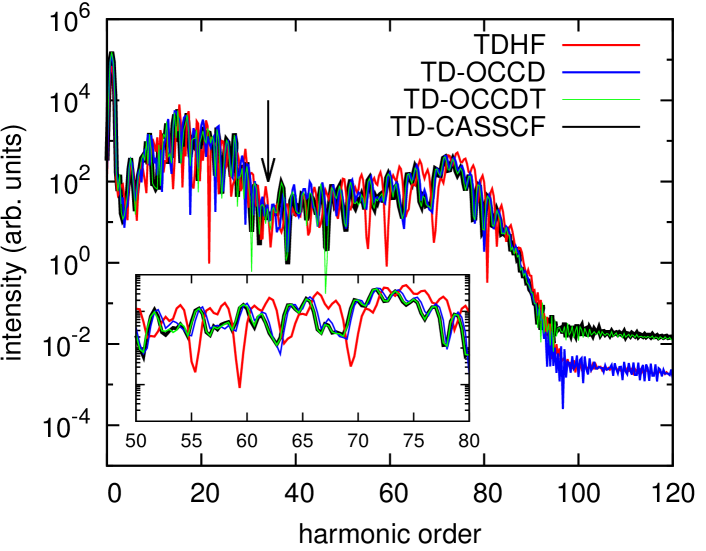
Figure 2: The HHG spectra of Ar exposed to a laser pulse with a wavelength of 800 nm and an intensity of 6$\times$10${}^{\textrm{14}}$ W/cm${}^{\textrm{2}}$. Comparison of the results of TDHF, TD-OCCD, TD-OCCDT, and TD-CASSCF methods. The inset shows a close-up of the spectra from 50th to 80th harmonic order.

Initial applications

Finally we report our initial application of the TD-OCC method to Ar atom in a strong laser field. We used the spherical FEDVR basis given as the product $Y_{lm}(\theta,\phi)f_{k}(r)$ of spherical harmonics $Y_{lm}$ with $l\leq l_{\rm max}$ and the FEDVR basis $f_{k}(r)$, which divides the range of radial coordinate $0<r<R_{\rm max}$ into finite elements of length 4 (with several finer elements near the nuclei), each supporting 23 local DVR functions. We first obtained the ground states of TDHF, TD-OCC, and TD-CASSCF methods by the imaginary time relaxation. For the latter two methods, the Ne core was kept frozen at HF orbitals and eight valence electrons were correlated among 13 optimized active orbitals, with their initial characters being $3s3p3d4p4s$.

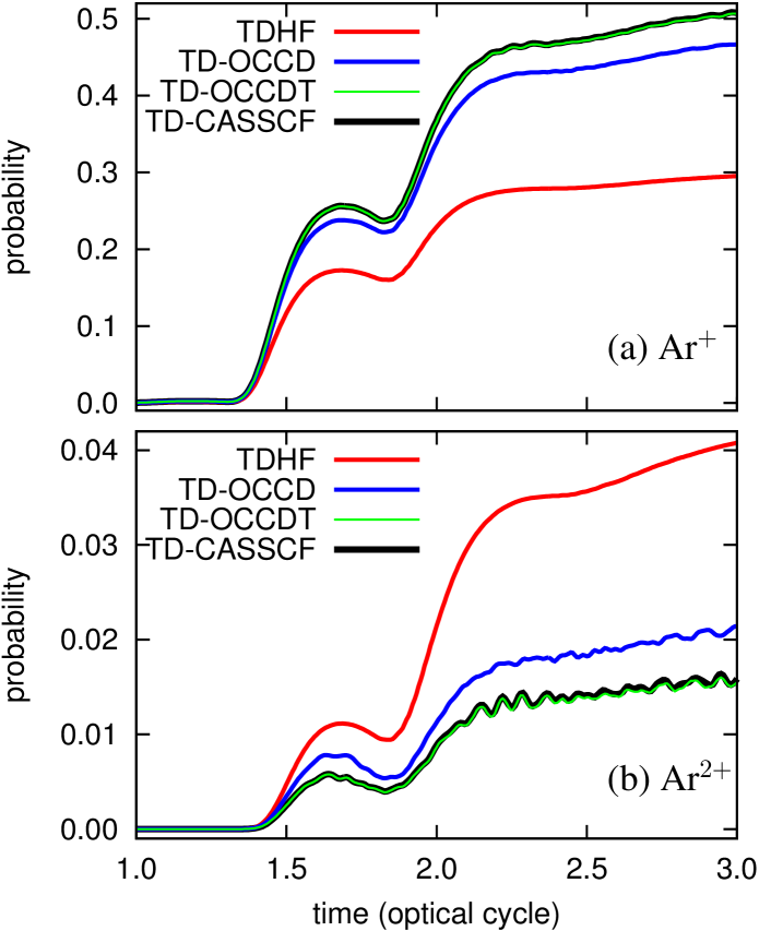
Figure 3: The probabilities, as a function of time, of finding one (a) and two (b) electrons outside a sphere of radius $R_{0}=20$ a.u. Results of TDHF, TD-OCCD, TD-OCCDT, and TD-CASSCF methods.

Starting from the ground states, we then simulated the electron dynamics of Ar atom subject to a linearly polarized (in the $z$ direction) laser pulse with a wavelength of 800 nm, a peak intensity of 6$\times$10${}^{\textrm{14}}$ W/cm${}^{\textrm{2}}$, and a foot-to-foot pulse duration of three optical cycles with a sin${}^{\textrm{2}}$-shaped envelope, within the dipole approximation in the velocity gauge. The EOMs are propageted using the fourth-order exponential Runge-Kutta method.Hochbruck and Ostermann (2010) The Ne core was frozen in all the methods and 13 active orbitals were propagated in TD-OCC and TD-CASSCF methods. The basis parameters were calibrated to achieve convergence with $R_{\rm max}=240$ (with the absorbing boundarySato and Ishikawa (2016)) and $l_{\rm max}=63$.

Figure 2 shows high-harmonic generation (HHG) spectra calculated as the modulus squared of the Fourier transform of the expectation value of the dipole acceleration $\langle d^{2}\hat{z}/dt^{2}\rangle(t)$ which, in turn, is obtained with the modified Ehrenfest expressionSato and Ishikawa (2016) using RDMs of Eq. (17). All methods predicted qualitatively similar spectra, with a minimum at 53 eV ($\approx$ 34th order, indicated with an arrow) close to the Cooper minimum of photoionization spectrum,Cooper (1962) which was experimentally observed.Wörner et al. (2009) The TDHF method, however, failed to reproduce fine structures of the TD-CASSCF spectrum especially at higher plateau as seen in the inset of Fig. 2. The description is largely improved by TD-OCCD, and the TD-OCCDT spectrum well reproduces the TD-CASSCF one in virtually all details.

We also compare the probabilities of finding one [Fig. 3 (a)] and two [Fig. 3 (b)] electron(s) outside a sphere of radius $R_{0}=20$, which measure the single and double ionization probabilities, respectively. These probabilites are much more sensitive to the description of correlated motions of electrons than HHG, which hinders a correct description with TDHF. The rapid converngence of TD-OCC results to the TD-CASSCF ones for such nonperturbatively nonlinear processes strongly promises the TD-OCC method to be a vital tool to investigate correlated high-field phenomena.

Summary

We have successfully formulated a new time-dependent coupled-cluster method called TD-OCC method, and implemented the first two, and the most important, series of approximations, TD-OCCD and TD-OCCDT. The present method is size extensive and gauge invariant, a polynomial cost-scaling alternative to the TD-MCSCF method. It would open new possibilities of high-accuracy first-principle investigations of multielectron dynamics in ever-unreachable large target systems. The rigorous derivation, details of the implementation, as well as other ansatz for TD-CC theories and comparison thereof, will be presented in a forthcoming article.Sato et al.