The Chazy XII Equation and Schwarz Triangle Functions

The Chazy XII Equation
and Schwarz Triangle Functions

Oksana BIHUN and Sarbarish CHAKRAVARTY O. Bihun and S. Chakravarty Department of Mathematics, University of Colorado, Colorado Springs, CO 80918, USA obihun@uccs.edu, schakrav@uccs.edu

Received June 21, 2017, in final form December 12, 2017; Published online December 25, 2017

Dubrovin [Lecture Notes in Math., Vol. 1620, Springer, Berlin, 1996, 120–348] showed that the Chazy XII equation $y^{\prime\prime\prime}-2yy^{\prime\prime}+3y^{\prime 2}=K(6y^{\prime}-y^{2})^{2}$, $K\in\mathbb{C}$, is equivalent to a projective-invariant equation for an affine connection on a one-dimensional complex manifold with projective structure. By exploiting this geometric connection it is shown that the Chazy XII solution, for certain values of $K$, can be expressed as $y=a_{1}w_{1}+a_{2}w_{2}+a_{3}w_{3}$ where $w_{i}$ solve the generalized Darboux–Halphen system. This relationship holds only for certain values of the coefficients $(a_{1},a_{2},a_{3})$ and the Darboux–Halphen parameters $(\alpha,\beta,\gamma)$, which are enumerated in Table 2. Consequently, the Chazy XII solution $y(z)$ is parametrized by a particular class of Schwarz triangle functions $S(\alpha,\beta,\gamma;z)$ which are used to represent the solutions $w_{i}$ of the Darboux–Halphen system. The paper only considers the case where $\alpha+\beta+\gamma<1$. The associated triangle functions are related among themselves via rational maps that are derived from the classical algebraic transformations of hypergeometric functions. The Chazy XII equation is also shown to be equivalent to a Ramanujan-type differential system for a triple $(\hat{P},\hat{Q},\hat{R})$.

Chazy; Darboux–Halphen; Schwarz triangle functions; hypergeometric

34M45; 34M55; 33C05

1 Introduction

In 1911, J. Chazy [10] considered the classification problem of all third order differential equations of the form $y^{\prime\prime\prime}=F(z,y,y^{\prime},y^{\prime\prime})$ possessing the Painlevé property, where the prime ^′ denotes ${\rm d}/{\rm d}z$, and $F$ is a polynomial in $y$, $y^{\prime}$, $y^{\prime\prime}$ and locally analytic in $z$. A differential equation in the complex plane is said to have the Painlevé property if its general solution has no movable branch points. In his work, Chazy introduced thirteen classes of equations referred to as Chazy classes I–XIII. Among these, classes III and XII are particularly interesting as their general solutions possess a movable barrier, i.e., a closed curve in the complex plane across which the solutions can not be analytically continued. That is, the solutions are analytic (or meromorphic) on either side of the barrier depending on the prescribed initial conditions. Both the Chazy III and XII equations can be expressed together as

$$y^{\prime\prime\prime}-2yy^{\prime\prime}+3y^{\prime 2}=K\big{(}6y^{\prime}-y^{2}\big{)}^{2},\qquad K=0\qquad\mbox{or}\qquad K=\frac{4}{36-k^{2}}.$$ (1.1)

The standard form for the Chazy XII equation is given by (1.1) with the parameter $K=4/(36-k^{2})$, whereas the Chazy III equation corresponds to $K=0$, and is the limiting case of Chazy XII as $k\to\infty$. Chazy [10] observed the remarkable fact that (1.1) is linearizable via the hypergeometric equation

$$s(s-1)\chi^{\prime\prime}+\big{(}{\textstyle\frac{7s}{6}}-{\textstyle\frac{1}{2}}\big{)}\chi^{\prime}+\big{(}{\textstyle\frac{1}{4k^{2}}}-{\textstyle\frac{1}{144}}\big{)}\chi=0,$$

for $k\in{\mathbb{C}}\cup\infty$, $k\neq 0$. He also showed that (1.1) possesses the Painlevé property when $K=0$ or when the value of the parameter $k$ is a positive integer such that $k>1$ and $k\neq 6$ (see also [12]). The $k=0$ case is linearizable by Airy’s equation $\chi^{\prime\prime}=cs\chi$, $c$ constant [11], and the limiting cases of $k=\pm 6$ can be solved via elliptic functions [10, 12]. For $K=0$ or for integer values $k>6$, the general solution of (1.1) possesses a movable natural barrier in the complex plane.

The Chazy III equation arises in mathematical physics in studies concerning magnetic monopoles [3], self-dual Yang–Mills and Einstein equations [8, 21], topological field theory [14], as well as special reductions of hydrodynamic type equations [16] and incompressible fluids [30]. The Chazy XII equation is related to the generalized Darboux–Halphen system [1, 2], which arises in reductions of self-dual Yang–Mills equations associated with the gauge group of diffeomorphism $\operatorname{Dif\/f}(S^{3})$ of a 3-sphere [9] as well as ${\rm SU}(2)$-invariant hypercomplex manifolds [22] with self-dual Weyl curvature [6]. More recently, the Chazy XII equation with specific values of the parameter $k$ has been linked to the study of vanishing Cartan curvature invariant for certain types of rank 2 distributions on a 5-manifold [28, 29]. Consequently, there has been renewed interest in the study of (1.1) and the singularity structure of its solutions in the complex plane. Interested readers are referred to the comprehensive works by Bureau [4], Clarkson and Olver [11] and Cosgrove [12].

A significant aspect of (1.1) is the fact that its general solutions can be expressed in terms of Schwarz triangle functions which define conformal mappings from the upper half complex plane onto a region bounded by three circular arcs (see, e.g., [24]). For $K=0$, solutions of the Chazy III equation are related to the automorphic forms associated with the modular group ${\rm SL}_{2}(\mathbb{Z})$ and its subgroups [7]. This fact can be traced back to the work of S. Ramanujan. In 1916, Ramanujan [25], [27, pp. 136–162] introduced certain functions $P(q)$, $Q(q)$, $R(q)$, $q:=e^{2\pi iz}$, $\operatorname{Im}(z)>0$, which correspond to the (first three) Eisenstein series associated with the modular group ${\rm SL}_{2}(\mathbb{Z})$. He showed that these functions satisfy the differential relations

$$\frac{1}{2\pi i}P^{\prime}(z)=\frac{P^{2}-Q}{12},\qquad\frac{1}{2\pi i}Q^{\prime}(z)=\frac{PQ-R}{3},\qquad\frac{1}{2\pi i}R^{\prime}(z)=\frac{PR-Q^{2}}{2}.$$ (1.2)

System (1.2) can be reduced to a single third order differential equation for $P(q)$. In fact, the function $y(z):=\pi iP(q)$ satisfies the Chazy III equation.

For $K\neq 0$, the solutions of the Chazy XII equation are also related to Schwarz functions automorphic on curvilinear triangles that tessellate the interior of the natural barrier for integer values of the parameter $k>6$. For $2\leq k\leq 5$ the solutions of (1.1) are expressed via the polyhedral functions which are rational functions associated with symmetry groups of solids (see, e.g., [17]).

In this paper, we primarily consider the Chazy XII equation (1.1) for integer values $k>6$. The main objective of this paper is to find all solutions $y(z)$ that are given in terms of Schwarz triangle functions. The central result to achieve this goal is the following:

If $y(z)=6Y(z)$ solves (1.1) with $K\neq 0$, then $Y(z)$ is a convex linear combination

$$Y(z)=\beta_{1}w_{1}+\alpha_{1}w_{2}+\gamma_{1}w_{3},\qquad\alpha_{1},\beta_{1},\gamma_{1}>0,\qquad\alpha_{1}+\beta_{1}+\gamma_{1}=1$$

of the variables $w_{1}$, $w_{2}$, $w_{3}$ satisfying the Darboux–Halphen system (2.9) with parameters $(\alpha{,}\beta{,}\gamma)$. The relationship holds only for special choices of $(\alpha_{1},\beta_{1})$ and $(\alpha,\beta,\gamma)$ listed in Table 2 of Section 3.3. The variables $w_{1}$, $w_{2}$, $w_{3}$ are expressed in terms of the Schwarz triangle function $s(z)=S(\alpha,\beta,\gamma;z)$ and its derivatives as shown in (2.11).

The above result is obtained by extending the geometric formulation of (1.1) by B. Dubrovin [14] to recast (1.1) as a purely algebraic relation. The Chazy XII solution $y(z)$ is expressed in a parametric form involving hypergeometric functions ${}_{2}F_{1}$

$$y=y(s),\qquad z=z(s),$$

where $s(z)=S(\alpha,\beta,\gamma;z)$ is the Schwarz triangle function (see Section  2.2 for details). Thus, Table 2 provides explicit parametrizations of the Chazy XII solutions in terms of a distinct family of Schwarz triangle functions. This family includes previously known functions, e.g., $S({\textstyle\frac{1}{2}},{\textstyle\frac{1}{3}},{\textstyle\frac{1}{k}};z)$, $6<k\in\mathbb{N}$ as well as some new cases. We believe that our approach is new, and that it can be applied to study similar nonlinear equations with natural barrier [5, 23].

The paper is organized as follows. Section 2.1 develops necessary geometric background on affine connections on a one-dimensional complex manifold with a projective structure following [14]. In Section 2.2, the generalized Darboux–Halphen system is introduced and its solutions in terms of Schwarz triangle functions are discussed. The connection between the Chazy XII equation and the generalized Darboux–Halphen system described in Section 3.1 leads to a purely algebraic formulation of (1.1). The solvability conditions of this algebraic system are analyzed in Section 3.2, and these lead to a classification of the Chazy XII solutions according to their pole structures inside the natural barrier. In Section 3.3, a Ramanujan-type triple of functions is introduced. These functions satisfy a system of first order equations that is similar to (1.2) and is equivalent to the Chazy XII equation. In Section 4.1, the Schwarz triangle function is presented as the inverse to the conformal map defined by the ratio of two linearly independent solutions of the hypergeometric equation. The parametrizations of the Ramanujan-like triple as well as the Chazy XII solution in terms of hypergeometric functions are also discussed here. Section 4.2 outlines the rational transformations between the distinct Schwarz functions parameterizing the Chazy XII solution. These rational maps are derived from the well-known algebraic transformations among the hypergeometric functions. In order to make the paper self-contained, we have included two appendices. Appendix A contains a proof of Lemma 3.1 introduced in Section 3.2, while Appendix B contains an elementary derivation of the radius of the natural barrier for the Chazy XII solution.

2 Background

2.1 Affine connection and projective structure

We begin this section by reviewing the relation between the solution $y(z)$ in (1.1) with affine connections on a one-dimensional complex manifold. We consider differential forms of order $m\in\mathbb{N}$ denoted by $f=f(z){\rm d}z^{m}$ on a one-dimensional complex manifold with local coordinate $z$, where $f(z)$ is a holomorphic (or meromorphic) function. Under the local change of coordinates $z\to\tilde{z}(z)$, $f$ transforms according to $f(z)dz^{m}=\tilde{f}(\tilde{z}){\rm d}\tilde{z}^{m}$. The covariant derivative of a $m$-differential is a $(m+1)$-differential $\nabla f$ defined by

$$\nabla f=\nabla f(z){\rm d}z^{m+1},\qquad\nabla f(z):=f^{\prime}(z)-m\eta(z)f(z),$$

where $\eta=\eta(z){\rm d}z$ is a holomorphic (or meromorphic) affine connection on the manifold. It follows from the transformation property of $\nabla f$ that $\eta$ must transform as

$$\tilde{\eta}(\tilde{z}){\rm d}\tilde{z}=\eta(z){\rm d}z-\big{(}\tilde{z}^{\prime\prime}(z)/\tilde{z}^{\prime}(z)\big{)}{\rm d}z.$$ (2.1)

The “curvature” associated with $\eta$ is defined by the quadratic differential $\Omega=~{}\Omega(z)dz^{2}$ as

$$\Omega(z):=\eta^{\prime}(z)-{\textstyle\frac{1}{2}}\eta(z)^{2}.$$

In fact, $\Omega$ is a projective connection transforming under local change of coordinates as

$$\tilde{\Omega}(\tilde{z}){\rm d}\tilde{z}^{2}=\Omega(z){\rm d}z^{2}-\{\tilde{z};z\}{\rm d}z^{2},\qquad\{\tilde{z},z\}:=\frac{\tilde{z}^{\prime\prime\prime}(z)}{\tilde{z}^{\prime}(z)}-\frac{3}{2}\left(\frac{\tilde{z}^{\prime\prime}(z)}{\tilde{z}^{\prime}(z)}\right)^{2},$$ (2.2)

where $\{\tilde{z},z\}$ is called the Schwarzian derivative. Under the projective (Möbius) transformations

$$z\to\tilde{z}=\frac{az+b}{cz+d},\qquad ad-bc\neq 0,$$

$\Omega$ transforms covariantly, i.e., $\Omega(z){\rm d}z^{2}=\tilde{\Omega}(\tilde{z}){\rm d}\tilde{z}^{2}$ because $\{\tilde{z},z\}=0$. Consequently, any $m$-differential of the form $Q=Q(z){\rm d}z^{m}$, where $Q(\Omega(z),\nabla\Omega(z),\nabla^{2}\Omega(z),\ldots)$ is a homogeneous polynomial of degree $m$ with $\deg\nabla^{r}\Omega=r+2$, transforms covariantly and an equation of the form $Q=0$ remains invariant under a projective transformation. It was shown in [14] that equation (1.1) corresponds to the projective-invariant equation $Q=0$ for $m=2$, i.e.,

$$\nabla^{2}\Omega+J\Omega^{2}=0$$ (2.3)

for any constant $J$. This yields the following third order differential equation for $\eta(z)$:

$$\eta^{\prime\prime\prime}-6\eta\eta^{\prime\prime}+9\eta^{\prime 2}+(J-12)\big{(}\eta^{\prime}-{\textstyle\frac{1}{2}}\eta^{2}\big{)}^{2}=0,$$ (2.4)

which reduces to (1.1) by setting $y=3\eta$ and $108K=(12-J)$. Thus, the Chazy III and Chazy XII equations (1.1) can be interpreted as a certain differential polynomial invariant of an affine connection in a one-dimensional complex manifold with a projective structure.

A projective structure on a one-dimensional complex manifold $M\subseteq\mathbb{CP}^{1}$ is defined by an atlas of local coordinates with transition functions given by Möbius transformations. In a local coordinate chart, the Möbius transformations are generated by the vector fields $\langle\partial_{z},z\partial_{z},z^{2}\partial_{z}\rangle$ isomorphic to the Lie algebra $\mathfrak{sl}_{2}(\mathbb{C})$. A nontrivial representation of $\mathfrak{sl}_{2}(\mathbb{C})$ is given by the vector fields $\langle u_{1}^{2}\partial_{s},u_{1}u_{2}\partial_{s},u_{2}^{2}\partial_{s}\rangle$ where $u_{1}(s)$, $u_{2}(s)$ is a pair of linearly independent solutions of the complex Schrödinger equation

$$u^{\prime\prime}+{\textstyle\frac{1}{4}}V(s)u=0,$$ (2.5)

(where the factor ${\textstyle\frac{1}{4}}$ is inserted for convenience). Then the identification of the vector field $\partial_{z}$ with $u_{1}^{2}\partial_{s}$ induces a local change of coordinates $s\to z(s)$ on $M$ via the ratio

$$z(s)=\frac{u_{2}(s)}{u_{1}(s)}.$$ (2.6)

If $M$ is not simply connected, the monodromy group $G\subset{\rm GL}_{2}({\mathbb{C}})$ resulting from the analytic extensions of the pair $(u_{2},u_{1})\to(au_{2}+bu_{1},cu_{2}+du_{1})$ along all possible closed loops in $M$ acts projectively on the ratio in (2.6) via the Möbius transformations

$$z\to\gamma(z):=\frac{az+b}{cz+d},\qquad\begin{pmatrix}a&b\\ c&d\end{pmatrix}\in G.$$ (2.7)

The projectivized monodromy group is the quotient group $\Gamma\cong G/\lambda I_{2}\subseteq{\rm PSL}_{2}({\mathbb{C}})$, where $I_{2}$ is the $2\times 2$ identity matrix. A different choice for the basis $(u_{1},u_{2})$ would lead to a different projective structure on $M$.

Note that the Schwarzian derivative is a differential invariant of the projective transformation, i.e., $\{\gamma(z);s\}=\{z;s\}$. For a projective structure induced by the Schrödinger equation (2.5), $z(s)$ satisfies the third order Schwarzian equation

$$\{z;s\}={\textstyle\frac{1}{2}}V(s),$$ (2.8a)

which can be linearized via (2.5) and (2.6). It follows that the inverse function $$s(z) M s(z)=s(\gamma(z)) \gamma\in\Gamma$$ (if it exists globally) is a projective invariant function on the manifold with the automorphism , , and satisfies

$$\{s;z\}+{\textstyle\frac{1}{2}}V(s)s^{\prime}(z)^{2}=0.$$ (2.8b)

An affine connection on the one-dimensional complex manifold $M$ can be defined uniquely by its trivialization $\eta(s)=0$ in the projective invariant coordinate $s$. Then the transformation $s\to z(s)=u_{2}(s)/u_{1}(s)$ in terms of the solutions of the Schrödinger equation leads to the following expression of the affine connection in the $z$-coordinate

$$\eta(z)=s^{\prime\prime}(z)/s^{\prime}(z)=-z^{\prime\prime}(s)/z^{\prime}(s)^{2}=2u_{1}(s)u_{1}^{\prime}(s),$$

using the transformation rule (2.1). Furthermore, from (2.2), the differential $\Omega(z)$ is then given in terms of the Schrödinger potential $V(s)$ as

$$\Omega(z)=\{s;z\}=-\{z;s\}/z^{\prime}(s)^{2}=-{\textstyle\frac{1}{2}}u_{1}^{4}(s)V(s).$$

Consequently, the solutions of the Chazy III and XII equations (1.1), which are equivalent to (2.4), can be expressed via the solutions and the potential of the complex Schrödinger equation (2.5). It is worth noting that if the affine connection is trivialized in a different coordinate $x(s)$ with ${\rm d}x=f(s){\rm d}s$, then from (2.1), $\eta(z){\rm d}z={\rm d}\log(f(s)s^{\prime}(z))$. We will utilize this fact and the geometric framework discussed above to construct a solution method in Section 3 for (1.1), by exploiting its relationship to another nonlinear differential system described below.

2.2 The Halphen system and Schwarz triangle functions

In 1881, Halphen considered a slight variant [20, p. 1405, equation (5)] of the following nonlinear differential system

$$w_{1}^{\prime}=-w_{2}w_{3}+w_{1}(w_{2}+w_{3})+\tau^{2},$$

$$w_{2}^{\prime}=-w_{3}w_{1}+w_{2}(w_{3}+w_{1})+\tau^{2},$$ (2.9)

$$w_{3}^{\prime}=-w_{1}w_{2}+w_{3}(w_{1}+w_{2})+\tau^{2},$$

$$\tau^{2}=\alpha^{2}(w_{1}-w_{2})(w_{2}-w_{3})+\beta^{2}(w_{2}-w_{1})(w_{1}-w_{3})+\gamma^{2}(w_{3}-w_{1})(w_{2}-w_{3}),$$

for functions $w_{i}(z)\neq w_{j}(z)$, $i\neq j$, where $i,j\in\{1,2,3\}$, and $\alpha$, $\beta$, $\gamma$ are constants. A special case of this equation with $\alpha=\beta=\gamma=0$ originally appeared in Darboux’s work of triply orthogonal surfaces on $\mathbb{R}^{3}$ in 1878 [13]. Its solution was given by Halphen [19] in 1881 in terms of hypergeometric functions. Subsequently, Chazy [10] showed that $y(z):=2(w_{1}+w_{2}+w_{3})$ satisfies the Chazy III equation introduced in Section 1. More recently, (2.9) was re-discovered as a certain symmetry reduction of the self-dual Yang–Mills equations, and was referred to as the generalized Darboux–Halphen (gDH) system [1, 2].

The gDH system can be solved via the Schrödinger equation (2.5) with the potential

$$V(s)=\frac{1-\alpha^{2}}{s^{2}}+\frac{1-\beta^{2}}{(s-1)^{2}}+\frac{\alpha^{2}+\beta^{2}-\gamma^{2}-1}{s(s-1)},$$ (2.10)

and defining a projective structure on $M$ via the ratio $z(s)$ in (2.6) as described in Section 2.1. Note that in this case (2.5) is a second order Fuchsian differential equation with three regular singular points, and $\alpha$, $\beta$, $\gamma$ are the exponent differences (for any pair of linearly independent solutions $u_{1}$ and $u_{2}$) prescribed at the singular points $0$, $1$ and $\infty$, respectively. The generators of the projectivized monodromy group $\Gamma$ are determined by the exponent differences. If the gDH variables $w_{1}(z)$, $w_{2}(z)$, $w_{3}(z)$ are expressed in terms of the projective invariant inverse function $s(z)$ (and its derivatives) as follows:

$$w_{1}=\frac{1}{2}\left[\log\left(\frac{s^{\prime}}{s}\right)\right]^{\prime},\quad w_{2}=\frac{1}{2}\left[\log\left(\frac{s^{\prime}}{s-1}\right)\right]^{\prime},\quad w_{3}=\frac{1}{2}\left[\log\left(\frac{s^{\prime}}{s(s-1)}\right)\right]^{\prime},$$ (2.11)

then a straightforward calculation shows that (2.9) reduces to the Schwarzian equation (2.8b) for $s(z)$, where the constants $\alpha$, $\beta$, $\gamma$ in $V(s)$ are the same as those appearing in $\tau^{2}$ of (2.9). Equation (2.8b) is equivalent to (2.8a) (after interchanging the dependent and independent variables) which is then reduced to (2.5). Thus, the gDH system can be effectively linearized by the Schrödinger equation (2.5) with the potential $V(s)$ given by (2.10).

The ratio $z(s)$ in (2.6) of any two linearly independent solutions $u_{1}$, $u_{2}$ of (2.5) with the potential $V(s)$ given by (2.10) defines a conformal mapping that was studied extensively by H.A. Schwarz [31] in 1873. The map $z(s)$ is, in general, branched at the regular singular points $s=0,1,\infty$. However, if the parameters $\alpha$, $\beta$, $\gamma$ are either zero or reciprocals of positive integers, and satisfy $\alpha+\beta+\gamma<1$, then the mapping $z(s)$ defines a plane region D, which is tessellated by an infinite number of non-overlapping hyperbolic, circular triangles on the complex $z$-plane. The interior of each triangle is an image of the upper (lower)-half $s$-plane under the map $z(s)$ and its analytic extensions, and is bounded by three circular arcs forming interior angles $\alpha\pi$, $\beta\pi$, and $\gamma\pi$ at the vertices $z(0)$, $z(1)$, and $z(\infty)$, respectively. Two adjacent triangles are obtained via Schwarz reflection principle, and are images of each other under reflection across the circular arc that forms their common boundary. In this case, the inverse $s(z)$ is a single-valued, meromorphic, automorphic function whose automorphism group is the projective monodromy group $\Gamma$ associated with (2.5) and (2.10). That is, $s(\gamma(z))=s(z)$ for all $\gamma\in\Gamma$ where $\gamma(z)$ is the Möbius transformation defined in (2.7). When the exponent differences satisfy the conditions prescribed above, $\Gamma$ is a discrete subgroup of ${\rm PSL}(2,{\mathbb{R}})$, and turns out to be the group of Möbius transformations generated by an even number of reflections across the boundaries of the circular triangles. This automorphic inverse function

$$s(z):=S(\alpha,\beta,\gamma;z)$$

is called the Schwarz triangle function, and the automorphism group $\Gamma$ is referred to as the triangle group. It is worth noting that if $\alpha$, $\beta$, $\gamma$ in (2.10) are either zero or reciprocals of positive integers, but either $\alpha+\beta+\gamma=1$ or $\alpha+\beta+\gamma>1$, then the map $z(s)$ in (2.6) tiles the $z$-plane either into infinitely many plane triangles, or the extended $z$-plane (Riemann sphere) into a finite number of spherical triangles, respectively. The triangle group $\Gamma$ is a simply or doubly periodic group when $\alpha+\beta+\gamma=1$, and corresponds to one of the four symmetry groups of the regular solids when $\alpha+\beta+\gamma>1$. A detailed discussion of the automorphic groups can be found in the monograph [17].

It follows from (2.8b) or from (2.5) with $V(s)$ as in (2.10) that the only possible singularities of $s(z)$ and its derivatives on the domain D are located at the vertices of each triangle where $s(z)$ takes the value of 0, 1, or $\infty$. The boundary of D in the $z$-plane is a $\Gamma$-invariant circle C which is orthogonal to all three sides of each triangle and its reflected images. This orthogonal circle C is the set of limit points for the automorphic group $\Gamma$, and corresponds to a dense set of essential singularities which form a natural barrier for the function $s(z)$. In its domain of existence D, the only possible singularities of $s(z)$ are poles which correspond to the vertices where $s(z)=\infty$.

In summary, when the parameters $\alpha$, $\beta$, $\gamma$ in (2.10) are either zero or reciprocals of positive integers and $\alpha+\beta+\gamma<1$, the general solution of (2.8b) is obtained as the unique inverse of the ratio

$$z(s)=\frac{au_{2}(s)+bu_{1}(s)}{cu_{2}(s)+du_{1}(s)},\qquad a,b,c,d\in{\mathbb{C}},\qquad ad-bc=1,$$ (2.12)

where $u_{1}$ and $u_{2}$ are two linearly independent solutions of (2.5). The solution is single-valued and meromorphic inside a disk in the extended $z$-plane, and can not be continued analytically across the boundary of the disk. This boundary is movable as its center and radius are completely determined by the initial conditions, which depend on the complex parameters $a$, $b$, $c$, $d$. Recently, a number of new nonlinear differential equations whose solutions possess movable natural boundaries have been found [5, 23]. These can be solved by first transforming them into a Schwarzian equation (2.8b) and then following the linearization scheme described above.

3 Chazy XII and triangle functions

In this section we present a solution method for the Chazy XII equation based on the geometric approach discussed in Section 2. Specifically, we exploit the fact that the Chazy XII equation in (1.1) is equivalent to the coordinate independent form in (2.3) for the quadratic differential $\Omega$. We express the affine connection $\eta$ associated with $\Omega$ via the gDH variables introduced in Section 2.2 so that the Chazy XII equation can be expressed in terms of the Schrödinger potential $V(s)$ in (2.10) and its derivatives, in a simple algebraic fashion. Then the solution of the Chazy XII equation is obtained via the Schwarz triangle function $S(\alpha,\beta,\gamma;z)$ for specific values of the triple $(\alpha,\beta,\gamma)$, which we identify. Recall that in this article we only consider the Chazy XII equation. The parametrization of the Chazy III equation by Schwarz triangle functions was studied in [7].

3.1 The gDH system and the Chazy XII equation

Note first from (2.11) and (2.1) that $2w_{i}={\rm d}\log(f_{i}(s)s^{\prime}(z))/{\rm d}z$ transforms as an affine connection that is trivialized in the coordinate $x_{i}(s)$ with ${\rm d}x_{i}=f_{i}(s){\rm d}s$ for

$$f_{1}(s)=\frac{1}{s},\qquad f_{2}(s)=\frac{1}{s-1},\qquad f_{3}(s)=\frac{1}{s(s-1)}.$$

In particular, under a Möbius transformation $z\to\gamma(z)$ given by (2.7) with $ad-bc=1$, $w_{i}$ transforms as

$$w_{i}(\gamma(z))=(cz+d)^{2}w_{i}(z)+c(cz+d),\qquad\gamma\in\Gamma,$$

which leaves the gDH system (2.9) invariant. Next let us define the function

$$y(z):=a_{1}w_{1}+a_{2}w_{2}+a_{3}w_{3},$$ (3.1)

in terms of the gDH variables $w_{i}$, where the coefficients $a_{i}$ are nonnegative constants. Then from (2.11), $y(z)$ can be expressed in terms of $s(z)$ and its derivatives as follows:

$$y(z)=\frac{p}{2}\,\frac{\phi^{\prime}(z)}{\phi(z)},\quad\qquad\phi(z)=\frac{s^{\prime}(z)}{s(z)^{1-\alpha_{1}}(s(z)-1)^{1-\beta_{1}}},$$ (3.2)

with $p:=a_{1}+a_{2}+a_{3}$, $\alpha_{1}:=a_{2}/p$ and $\beta_{1}:=a_{1}/p$ and $0\leq\alpha_{1},\beta_{1}\leq 1$. If we set $p=6$ above, then it is possible to define an affine connection $\eta$ such that in the $z$-coordinate,

$$\eta(z)=\frac{y(z)}{3}=\frac{{\rm d}\log(\phi)}{{\rm d}z}.$$

It follows from (2.1) that $\eta$ is trivialized in the coordinate $x$ such that ${\rm d}x=\phi(z){\rm d}z=f(s){\rm d}s$ where $f(s)=s^{-1+\alpha_{1}}(s-1)^{-1+\beta_{1}}$. Moreover, in the $s$-coordinate,

$$\eta(s)=(\log f)^{\prime}(s)=-\frac{1-\alpha_{1}}{s}-\frac{1-\beta_{1}}{s-1},\qquad\Omega(s)=\eta^{\prime}(s)-{\textstyle\frac{1}{2}}\eta^{2}(s),$$ (3.3)

which are rational functions of $s$. The curvature in the $z$-coordinate is obtained using the transformation property (2.2) as

$$\Omega(z)=(\Omega(s)-\{z;s\})s^{\prime}(z)^{2}=(\Omega(s)-{\textstyle\frac{1}{2}}V(s))s^{\prime}(z)^{2}:=-V_{2}(s)s^{\prime}(z)^{2},$$

where the second equality above follows from (2.8a) with $V(s)$ as in (2.10). Then the covariant derivatives of the quadratic differential $\Omega$ are given by the transformation rule

$$\nabla^{m}\Omega(z)=-(\nabla^{m}V_{2}(s))s^{\prime}(z)^{m+2}:=-V_{m+2}(s)s^{\prime}(z)^{m+2},\qquad m\geq 1,$$

where $V_{m+2}(s)$ are rational functions of $s$ defined recursively for $n\geq 2$ as

$$V_{n+1}(s)=\nabla V_{n}(s)=V_{n}^{\prime}(s)-n\eta(s)V_{n}(s),\qquad V_{2}(s)={\textstyle\frac{1}{2}}V(s)-\eta^{\prime}(s)+{\textstyle\frac{1}{2}}\eta(s)^{2},$$ (3.4)

with $\eta(s)$ defined in (3.3).

Our next goal is to derive conditions under which $\Omega(z)$ will satisfy the projective-invariant equation (2.3), equivalently, the affine connection $\eta(z)$ will satisfy (2.4). Then the function $y(z)=3\eta(z)$ defined in (3.2) with $p=6$ will solve the Chazy XII equation in (1.1). Henceforth, the value $p=6$ will be used throughout the rest of this article.

It follows from the expressions for $\Omega(z)$ and its covariant derivatives obtained above, that for $m=2$, (2.3) implies a simple algebraic relation between rational functions $V_{2}(s)$ and $V_{4}(s)$, namely,

$$V_{4}(s)=JV_{2}^{2}(s),\qquad J\neq 12,$$ (3.5)

that should hold for all $s$. This condition imposes certain restrictions on the parameters $(\alpha,\beta,\gamma)$ and $(\alpha_{1},\beta_{1})$ appearing in the functions $V_{2}(s)$ and $V_{4}(s)$. It is worth pointing out here that (3.5) together with (3.1) lead to the central result advertised in Section 1.

In what follows, we will systematically determine the sets of parameters for which (3.5) holds. In particular, we will identify the values of the triple $(\alpha,\beta,\gamma)$ in the Schwarz triangle functions $S(\alpha,\beta,\gamma;z)$ which determine the solution of the Chazy XII equation $y(z)$ via (3.2).

3.2 The Schwarz function parametrization

From equations (2.10), (3.3) and (3.4), the rational function $V_{2}(s)$ can be written as

$$V_{2}(s)=\frac{1}{2}\left[\frac{A}{s^{2}}+\frac{B}{(s-1)^{2}}+\frac{C}{s(s-1)}\right],$$

$$A=\alpha_{1}^{2}-\alpha^{2},\qquad B=\beta_{1}^{2}-\beta^{2},\qquad C=\gamma_{1}^{2}-A-B-\gamma^{2},$$ (3.6)

where the parameters $(\alpha_{1},\beta_{1},\gamma_{1})$ are defined as follows:

$$\alpha_{1}=\frac{a_{2}}{6},\qquad\beta_{1}=\frac{a_{1}}{6},\qquad\gamma_{1}=\frac{a_{3}}{6},\qquad 0\leq\alpha_{1},\beta_{1},\gamma_{1}\leq 1,\qquad\alpha_{1}+\beta_{1}+\gamma_{1}=1.$$ (3.7)

Then $V_{4}(s)$ is readily computed from the recurrence relation in (3.4). Upon substituting the expressions for $V_{2}(s)$ and $V_{4}(s)$ into (3.5) and rationalizing the resulting expression, one finds that (3.5) is satisfied if and only if

$$u_{1}s^{4}+u_{2}s^{3}(s-1)+u_{3}s^{2}(s-1)^{2}+u_{4}s(s-1)^{3}+u_{5}(s-1)^{4}=0$$

for all values of $s$. The last identity is equivalent to the vanishing of the coefficients $u_{i}$, i.e.,

$$u_{1}:=JB^{2}-12B\beta_{1}^{2}=0,$$ (3.8a)

$$u_{2}:=2JBC-4[(1-\alpha_{1})(1-6\beta_{1})B+{\textstyle\frac{1}{2}}(1-2\beta_{1})(1-3\beta_{1})C]=0,$$ (3.8b)

$$u_{3}:=J(2AB+C^{2})-4\big{[}(2-3\beta_{1})(1-\beta_{1})A+(2-3\alpha_{1})(1-\alpha_{1})B$$

$$\hphantom{u_{3}:=}{}+{\textstyle\frac{1}{2}}[(2-3\beta_{1})(1-2\alpha_{1})+(2-3\alpha_{1})(1-2\beta_{1})]C\big{]}=0,$$ (3.8c)

$$u_{4}:=2JAC-4[(1-\beta_{1})(1-6\alpha_{1})A+{\textstyle\frac{1}{2}}(1-2\alpha_{1})(1-3\alpha_{1})C]=0,$$ (3.8d)

$$u_{5}:=JA^{2}-12A\alpha_{1}^{2}=0.$$ (3.8e)

System (3.8) represents a set of coupled, algebraic equations for the parameters $(\alpha,\beta,\gamma)$, $(\alpha_{1},\beta_{1})$ and $J$ subject to the conditions

$$\alpha,\beta,\gamma\in\big{\{}{\textstyle\frac{1}{n}},\,n\in\mathbb{N}\big{\}}\cup\{0\},\qquad\alpha+\beta+\gamma<1,\qquad 0\leq\alpha_{1},\beta_{1}\leq 1,$$ (3.9)

and $J\neq 12$. The case $J=0$ corresponds to $K={\textstyle\frac{1}{9}}$ or $k=0$ in (1.1). The Chazy XII equation for this case can be linearized via Airy’s equation as mentioned in Section 1. Hence, the $J=0$ case is distinct from the cases considered here which correspond to Schrödinger potential $V(s)$ in (2.10) with three regular singular points. Furthermore, the following lemma is proven in Appendix A.

Lemma 3.1.

If $J=0$, then (3.8) has no admissible solution satisfying conditions (3.9).

Henceforth, we take $J\neq 0$ through the remainder of the main text of this paper.

Lemma 3.2.

If a triple $(\alpha,\beta,\gamma)$ of non-negative numbers satisfying $\alpha+\beta+\gamma<1$ solves the system (3.8) with $J\neq 12$, then $\alpha\neq 0$, $\beta\neq 0$, and $\gamma\neq 0$.

Proof.

If $\alpha=0$, then $A=\alpha_{1}^{2}$ from (3.6). The condition (3.8e) with $J\neq 12$ implies $\alpha_{1}=0$. Hence, $A=0$. Then equations (3.8c) and (3.8d) imply $B=0$ and $C=0$. Consequently, $\beta=\beta_{1}$, $\gamma=\gamma_{1}$ from (3.6). Therefore, $\beta+\gamma=\beta_{1}+\gamma_{1}=1$ contradicting $\alpha+\beta+\gamma<1$.

If $\beta=0$, the proof is similar to above, starting from condition (3.8a) first, then using equations (3.8b) and (3.8c).

If $\gamma=0$ then $D:=A+B+C=\gamma_{1}^{2}$. The condition $\sum\limits_{i=1}^{5}u_{i}=0$ in (3.8) yields $JD^{2}=12\gamma_{1}^{2}D$, which implies that $\gamma_{1}=0$. Hence, $\alpha_{1}+\beta_{1}=1$ and $D=0$. Using the last condition to eliminate $C$ from (3.8b) and (3.8d), one obtains

$$JAB=(1-2\beta_{1})(1-3\beta_{1})A-(1-6\beta_{1})(1-2\alpha_{1}-\beta_{1})B,$$ (3.10a)

$$JAB=-(1-6\alpha_{1})(1-2\beta_{1}-\alpha_{1})A+(1-2\alpha_{1})(1-3\alpha_{1})B,$$ (3.10b)

where (3.8a) and (3.8e) are also used to eliminate terms involving $A^{2}$ and $B^{2}$. It follows from (3.10a) and (3.10b) together with $\alpha_{1}+\beta_{1}=1$ that if either $A=0$, or $B=0$, then both $A$ and $B$ vanish. Hence, $\alpha+\beta=\alpha_{1}+\beta_{1}=1$, which contradicts $\alpha+\beta+\gamma<1$.

Finally, let $A\neq 0$ and $B\neq 0$. Then (3.8e) and (3.8a) imply that $JA=12\alpha_{1}^{2}$, $JB=12\beta_{1}^{2}$. Substituting these into (3.10a) and (3.10b) to eliminate $A$ and $B$, yields two equations for $\alpha_{1}$ and $\beta_{1}$. The resulting equations have no solution $(\alpha_{1},\beta_{1})$ that satisfies the condition $\alpha_{1}+\beta_{1}=1$. Thus, $\gamma$ can not be 0. ∎

One can also make the inequalities for $\alpha_{1}$, $\beta_{1}$, $\gamma_{1}$ in (3.7) strict, i.e., $0<\alpha_{1},\beta_{1},\gamma_{1}<1$.

Lemma 3.3.

If $\alpha_{1}$, $\beta_{1}$, $\gamma_{1}$ satisfy (3.7) and solve the system (3.8) with $(\alpha,\beta,\gamma)$ as in Lemma 3.2, then $\alpha_{1},\beta_{1},\gamma_{1}\notin\{0,1\}$.

Proof.

If $\alpha_{1}=0$, then it follows from (3.8e) that $A=0$. Then, (3.6) implies that $\alpha=\alpha_{1}=0$, contradicting Lemma 3.2. Thus $\alpha_{1}\neq 0$. A similar argument starting from (3.8a) shows that $\beta_{1}\neq 0$.

If $\alpha_{1}=1$, then (3.7) implies that $\beta_{1}=0$, which is not possible. Similarly, $\beta_{1}=1$ or $\gamma_{1}=1$ is not possible.

Finally, assume that $\gamma_{1}=0$. Since $JD^{2}=12\gamma_{1}^{2}D$ where $D:=A+B+C$ (see Lemma 3.2), it follows that $D=0$. Then, (3.6) implies that $\gamma=\gamma_{1}=0$, contradicting Lemma 3.2. ∎

Lemma 3.2 implies that $\alpha,\beta,\gamma\in\{{\textstyle\frac{1}{n}},\,n\in\mathbb{N}\}$ in (3.9). Let $s(z)=S(\alpha,\beta,\gamma;z)$ be the triangle function associated with those parameters, and let $z_{0}$ be a vertex of a triangle in the domain of existence D of $s(z)$ such that $s(z_{0}):=s_{0}\in\{0,1,\infty\}$. The map $z(s)$ defined via the equations (2.6), (2.5) and (2.10), behaves locally near $s=s_{0}$ as (see, e.g., [24])

$$z(s)=z_{0}+(s-s_{0})^{\mu}\psi_{1}(s),\qquad s_{0}\in\{0,1\}\qquad\mbox{and}$$

$$z(s)=z_{0}+s^{-\mu}\psi_{2}\big{(}s^{-1}\big{)},\qquad s_{0}=\infty,$$

where $\psi_{i}$ is analytic near $s_{0}$ with $\psi_{i}(s_{0})\neq 0$, and $\mu\in\{\alpha,\beta,\gamma\}$ is the corresponding exponent difference at the singular point $s_{0}$. Consequently, the inverse $s(z)$ is single-valued function defined locally as

$$s(z)=s_{0}+(z-z_{0})^{m}\phi_{1}(z),\qquad z_{0}\in\{z(0),z(1)\}\qquad\mbox{and}$$

$$s(z)=(z-z_{0})^{-m}\phi_{2}(z),\qquad z_{0}=z(\infty),$$

where $\phi_{i}(z)$ is analytic in the neighborhood of $z=z_{0}$ with $\phi_{i}(z_{0})\neq 0$, and $m=\mu^{-1}\in\mathbb{N}$. Thus, $s-s_{0}$ has a zero of order ${\textstyle\frac{1}{\alpha}}$, ${\textstyle\frac{1}{\beta}}$ at the vertices $z_{0}=z(0),z(1)$, respectively, and $s(z)$ has a pole of order ${\textstyle\frac{1}{\gamma}}$ at the vertex $z_{0}=z(\infty)$ of each triangle in the domain D. As mentioned earlier in Section 2, it is sufficient to examine the behavior of the function $s(z)$ and its derivatives near the vertices $z(0)$, $z(1)$, and $z(\infty)$ of just one triangle inside the domain D. The Schwarz reflection principle and the automorphic property then ensure that $s(z)$ will have the same behavior at the vertices of the reflected triangles in D. A straightforward calculation using the above behavior of $s(z)$ in (3.2) shows that $y(z)$ is a meromorphic function in D with simple poles at the vertices $z(0)$, $z(1)$, $z(\infty)$ of each triangle in D with the residues

$$\operatorname{Res}_{z(0)}=3({\textstyle\frac{\alpha_{1}}{\alpha}}-1),\qquad\operatorname{Res}_{z(1)}=3({\textstyle\frac{\beta_{1}}{\beta}}-1),\qquad\operatorname{Res}_{z(\infty)}=3({\textstyle\frac{\gamma_{1}}{\gamma}}-1).$$

Of course, at the boundary of the domain D, $y(z)$ inherits the same natural barrier of essential singularities as the function $s(z)$. Note that it is possible for $y(z)$ to be analytic at a vertex $z_{0}$ in the interior of D provided that the residue vanishes at $z_{0}$, i.e., if either $\alpha=\alpha_{1}$, $\beta=\beta_{1}$, or $\gamma=\gamma_{1}$. However, it is impossible for all three residues to vanish simultaneously because then $\alpha+\beta+\gamma=\alpha_{1}+\beta_{1}+\gamma_{1}=1$, which violates the condition $\alpha+\beta+\gamma<1$ in (3.9). The discussion above concerning the singularity structure of $y(z)$ in the interior of its domain of definition D can be summarized in the following proposition.

Proposition 3.4.

The solution $y(z)$ of the Chazy XII equation given by (3.2) in terms of the triangle function $s(z)=S(\alpha,\beta,\gamma;z)$ where $\alpha,\beta,\gamma$ satisfy (3.9), is meromorphic with only simple poles inside its domain of definition D. These poles can only occur at the vertices $z(0)$, $z(1)$ and $z(\infty)$ of the circular triangles tessellating the domain D. Moreover, $y(z)$ must have at least one simple pole at one of the vertices of each triangle.

Hence, there are three distinct cases resulting from Proposition 3.4, namely, $y(z)$ has a simple pole at (1)  only one vertex $z_{0}\in\{z(0),z(1),z(\infty)\}$, (2)  only two of the three vertices, and (3)  all three vertices. The admissible parameters that satisfy (3.8) can be determined by considering each case separately.

Case 1. Suppose $y(z)$ is analytic at $z(0)$ and $z(1)$, and has a simple pole only at $z(\infty)$ on each triangle in D. Then the vanishing of residues at $z(0)$ and $z(1)$ is equivalent to $\alpha=\alpha_{1}$ and $\beta=\beta_{1}$, which implies that $A=B=0$. Note however that $C\neq 0$ since $\operatorname{Res}_{z(\infty)}\neq 0$. In this case (3.8a) and (3.8e) are identically satisfied, while (3.8b) and (3.8d) imply that $(1-2\alpha_{1})(1-3\alpha_{1})=(1-2\beta_{1})(1-3\beta_{1})=0$. Hence,

$$(\alpha,\beta)\in\left\{\big{(}{\textstyle\frac{1}{2}},{\textstyle\frac{1}{2}}\big{)},\big{(}{\textstyle\frac{1}{2}},{\textstyle\frac{1}{3}}\big{)},\big{(}{\textstyle\frac{1}{3}},{\textstyle\frac{1}{2}}\big{)}\big{(}{\textstyle\frac{1}{3}},{\textstyle\frac{1}{3}}\big{)}\right\}.$$

Since the subcase $\alpha=\beta={\textstyle\frac{1}{2}}$ is not admissible due to the condition $\alpha+\beta+\gamma<1$, and the subcases $(\alpha,\beta)\in\{({\textstyle\frac{1}{2}},{\textstyle\frac{1}{3}}),({\textstyle\frac{1}{3}},{\textstyle\frac{1}{2}})\}$ are the same modulo a vertex permutation, there are only two distinct subcases, namely, $(\alpha,\beta)=({\textstyle\frac{1}{2}},{\textstyle\frac{1}{3}})$ and $(\alpha,\beta)=({\textstyle\frac{1}{3}},{\textstyle\frac{1}{3}})$.

If $(\alpha,\beta)=({\textstyle\frac{1}{2}},{\textstyle\frac{1}{3}})$, the remaining condition (3.8c) yields $JC={\textstyle\frac{1}{3}}$. Choosing $\gamma={\textstyle\frac{1}{k}}$, $k\in\mathbb{N}$, gives $J=12k^{2}/(k^{2}-36)$, which is consistent with the value of $K$ in (1.1). Recall (from the definition below (2.4)) that $K=(12-J)/108$.

If $(\alpha,\beta)=({\textstyle\frac{1}{3}},{\textstyle\frac{1}{3}})$, then (3.8c) implies that $JC={\textstyle\frac{4}{3}}$. In this case, choosing $\gamma={\textstyle\frac{1}{k}}$, $k\in\mathbb{N}$ gives $J=12k^{2}/(k^{2}-9)$ so that $K=1/(9-k^{2})$, which is different from the value used by Chazy in (1.1). However, the rescaling $k\to{\textstyle\frac{k}{2}}$ restores the value of $K$ in (1.1) while modifying the value of $\gamma$ to $\gamma={\textstyle\frac{2}{k}}$. If the simple pole of $y(z)$ is chosen to be at $z(0)$ or $z(1)$ instead, the values of the parameters are simply permuted. Thus, modulo permutations, there are two possible sets of admissible parameters:

$$(i)\quad (\alpha,\beta,\gamma)=\big{(}{\textstyle\frac{1}{2}},{\textstyle\frac{1}{3}},{\textstyle\frac{1}{k}}\big{)},\qquad(\alpha_{1},\beta_{1},\gamma_{1})=\big{(}{\textstyle\frac{1}{2}},{\textstyle\frac{1}{3}},{\textstyle\frac{1}{6}}\big{)},$$

$$(ii)\quad (\alpha,\beta,\gamma)=\big{(}{\textstyle\frac{1}{3}},{\textstyle\frac{1}{3}},{\textstyle\frac{2}{k}}\big{)},\qquad(\alpha_{1},\beta_{1},\gamma_{1})=\big{(}{\textstyle\frac{1}{3}},{\textstyle\frac{1}{3}},{\textstyle\frac{1}{3}}\big{)},$$

for the same value of $K$ as in (1.1), and the rescaled ($k\to 2k$) version of subcase (ii) above.

Case 2. Suppose now $y(z)$ is analytic at only one vertex $z(0)$ and has a simple pole at each of $z(1)$ and $z(\infty)$. Then $\alpha=\alpha_{1}$, which means $A=0$, so that (3.8e) is automatically satisfied. Here, $B\neq 0$ and $B+C\neq 0$ since the residues at $z(1)$ and $z(\infty)$ do not vanish. Then (3.8d) leads to three subcases: (i) $\alpha_{1}={\textstyle\frac{1}{2}}$, (ii) $\alpha_{1}={\textstyle\frac{1}{3}}$, and (iii) $C=0$.

In the case where $\alpha_{1}={\textstyle\frac{1}{2}}$, one solves first for $\beta_{1}$, then for $B$ and $B+C$ from the remaining equations in (3.8). The admissible values of the parameters up to a permutation, are $\beta_{1}={\textstyle\frac{1}{6}}$, and $(\alpha,\beta,\gamma)=({\textstyle\frac{1}{2}},{\textstyle\frac{1}{k}},{\textstyle\frac{2}{k}})$, $k\in\mathbb{N}$ with the value of $K$ as in (1.1). However, one also obtains $(\alpha,\beta,\gamma)=({\textstyle\frac{1}{2}},{\textstyle\frac{1}{2k}},{\textstyle\frac{1}{k}})$ with $K=1/(9-k^{2})$ as in Case 1 above, which can be rescaled via $k\to{\textstyle\frac{k}{2}}$ to Chazy’s choice for $K$.

If $\alpha_{1}={\textstyle\frac{1}{3}}$, a similar analysis as above yields $\beta_{1}={\textstyle\frac{1}{6}}$, and $(\alpha,\beta,\gamma)=({\textstyle\frac{1}{3}},{\textstyle\frac{1}{k}},{\textstyle\frac{3}{k}})$, $k\in\mathbb{N}$ with $K$ as in (1.1). There is also a second case with $(\alpha,\beta,\gamma)=({\textstyle\frac{1}{3}},{\textstyle\frac{1}{3k}},{\textstyle\frac{1}{k}})$ and $K=4/(36-9k^{2})$, which can be rescaled back to the previous case via $k\to{\textstyle\frac{k}{3}}$.

Finally, if $C=0$, (3.8c) reduces to $(2-3\alpha_{1})(1-\alpha_{1})B=0$. Therefore, $\alpha_{1}={\textstyle\frac{2}{3}}$ since $\alpha_{1}=\alpha\neq 1$ and $B\neq 0$. The remaining equations in (3.8) yield $\beta_{1}={\textstyle\frac{1}{6}}$, $\beta=\gamma={\textstyle\frac{1}{k}}$, $k\in\mathbb{N}$ with $K$ as in (1.1).

Case 3. If $y(z)$ has a simple pole at each of the vertices $z(0)$, $z(1)$ and $z(\infty)$, then $A\neq 0$, $B\neq 0$, and $A+B+C\neq 0$. The equations (3.8a) and (3.8e) imply, respectively, that $JB=12\beta_{1}^{2}$ and $JA=12\alpha_{1}^{2}$. Substituting these into (3.8b) and (3.8d), one obtains

$$(1-6\beta_{1})\big{[}2(1-\alpha_{1})B+(1+\beta_{1})C\big{]}=0,$$

$$(1-6\alpha_{1})\big{[}2(1-\beta_{1})A+(1+\alpha_{1})C\big{]}=0.$$

The above equations lead to four distinct subcases: (i) $\alpha_{1}=\beta_{1}={\textstyle\frac{1}{6}}$, (ii) $\alpha_{1}={\textstyle\frac{1}{6}}$, $\beta_{1}\neq{\textstyle\frac{1}{6}}$, (iii) $\alpha_{1}\neq{\textstyle\frac{1}{6}}$, $\beta_{1}={\textstyle\frac{1}{6}}$, (iv) $\alpha_{1}\neq{\textstyle\frac{1}{6}},\beta_{1}\neq{\textstyle\frac{1}{6}}$. From the remaining condition (3.8c) and the above equations one finds that the first three subcases yield, modulo permutations, only one distinct set of admissible parameter values given by

$$(\alpha,\beta,\gamma)=\big{(}{\textstyle\frac{1}{k}},{\textstyle\frac{1}{k}},{\textstyle\frac{4}{k}}\big{)},\qquad k\in\mathbb{N},\qquad(\alpha_{1},\beta_{1},\gamma_{1})=\big{(}{\textstyle\frac{1}{6}},{\textstyle\frac{1}{6}},{\textstyle\frac{2}{3}}\big{)},$$

with $K$ as in (1.1). Like the previous two cases, an additional set $(\alpha,\beta,\gamma)=({\textstyle\frac{1}{4k}},{\textstyle\frac{1}{4k}},{\textstyle\frac{1}{k}})$ with $K=1/(9-4k^{2})$ is also found by first choosing $\gamma={\textstyle\frac{1}{k}}$ and then solving for $\alpha$, $\beta$. This case can be reduced to the one displayed above by the rescaling $k\to{\textstyle\frac{k}{4}}$.

Subcase (iv) leads to $\alpha_{1}=\beta_{1}$ and $\alpha=\beta$. Using condition (3.8c), one obtains the equilateral triangle corresponding to $\alpha=\beta=\gamma={\textstyle\frac{2}{k}}$, $k\in\mathbb{N}$ and $\alpha_{1}=\beta_{1}=\gamma_{1}={\textstyle\frac{1}{3}}$ with $K$ as in (1.1). It is also possible to choose $\alpha=\beta=\gamma={\textstyle\frac{1}{k}}$ for the same values of $\alpha_{1}$ and $\beta_{1}$ but with $K=1/(9-k^{2})$. These are related by the rescaling $k\to{\textstyle\frac{k}{2}}$.

Case	$(\alpha,\beta,\gamma)$	$(\alpha_{1},\beta_{1})$	$K$	$(\operatorname{Res}_{z(0)},\operatorname{Res}_{z(1)},\operatorname{Res}_{z(\infty)})$2pt2pt
1(a)	$({\textstyle\frac{1}{2}},{\textstyle\frac{1}{3}},{\textstyle\frac{1}{k}})$	$({\textstyle\frac{1}{2}},{\textstyle\frac{1}{3}})$	${\textstyle\frac{4}{36-k^{2}}}$	$(0,0,{\textstyle\frac{k-6}{2}})$ 2pt2pt
1(b)	$({\textstyle\frac{1}{3}},{\textstyle\frac{1}{3}},{\textstyle\frac{2}{k}})$	$({\textstyle\frac{1}{3}},{\textstyle\frac{1}{3}})$	${\textstyle\frac{4}{36-k^{2}}}$	$(0,0,{\textstyle\frac{k-6}{2}})$ 2pt2pt
1(b)∗	$({\textstyle\frac{1}{3}},{\textstyle\frac{1}{3}},{\textstyle\frac{1}{k}})$	$({\textstyle\frac{1}{3}},{\textstyle\frac{1}{3}})$	${\textstyle\frac{1}{9-k^{2}}}$	$(0,0,k-3)$ 2pt2pt
2(a)	$({\textstyle\frac{1}{2}},{\textstyle\frac{1}{k}},{\textstyle\frac{2}{k}})$	$({\textstyle\frac{1}{2}},{\textstyle\frac{1}{6}})$	${\textstyle\frac{4}{36-k^{2}}}$	$(0,{\textstyle\frac{k-6}{2}},{\textstyle\frac{k-6}{2}})$ 2pt2pt
2(a)∗	$({\textstyle\frac{1}{2}},{\textstyle\frac{1}{2k}},{\textstyle\frac{1}{k}})$	$({\textstyle\frac{1}{2}},{\textstyle\frac{1}{6}})$	${\textstyle\frac{1}{9-k^{2}}}$	$(0,k-3,k-3)$ 2pt2pt
2(b)	$({\textstyle\frac{1}{3}},{\textstyle\frac{1}{k}},{\textstyle\frac{3}{k}})$	$({\textstyle\frac{1}{3}},{\textstyle\frac{1}{6}})$	${\textstyle\frac{4}{36-k^{2}}}$	$(0,{\textstyle\frac{k-6}{2}},{\textstyle\frac{k-6}{2}})$ 2pt2pt
2(b)∗	$({\textstyle\frac{1}{3}},{\textstyle\frac{1}{3k}},{\textstyle\frac{1}{k}})$	$({\textstyle\frac{1}{3}},{\textstyle\frac{1}{6}})$	${\textstyle\frac{4}{9(4-k^{2})}}$	$(0,{\textstyle\frac{3k-6}{2}},{\textstyle\frac{3k-6}{2}})$ 2pt2pt
2(c)	$({\textstyle\frac{2}{3}},{\textstyle\frac{1}{k}},{\textstyle\frac{1}{k}})$	$({\textstyle\frac{2}{3}},{\textstyle\frac{1}{6}})$	${\textstyle\frac{4}{36-k^{2}}}$	$(0,{\textstyle\frac{k-6}{2}},{\textstyle\frac{k-6}{2}})$ 2pt2pt
3(a)	$({\textstyle\frac{1}{k}},{\textstyle\frac{1}{k}},{\textstyle\frac{4}{k}})$	$({\textstyle\frac{1}{6}},{\textstyle\frac{1}{6}})$	${\textstyle\frac{4}{36-k^{2}}}$	$({\textstyle\frac{k-6}{2}},{\textstyle\frac{k-6}{2}},{\textstyle\frac{k-6}{2}})$ 2pt2pt
3(a)∗	$({\textstyle\frac{1}{4k}},{\textstyle\frac{1}{4k}},{\textstyle\frac{1}{k}})$	$({\textstyle\frac{1}{6}},{\textstyle\frac{1}{6}})$	${\textstyle\frac{1}{9-4k^{2}}}$	$(2k-3,2k-3,2k-3)$ 2pt2pt
3(b)	$({\textstyle\frac{2}{k}},{\textstyle\frac{2}{k}},{\textstyle\frac{2}{k}})$	$({\textstyle\frac{1}{3}},{\textstyle\frac{1}{3}})$	${\textstyle\frac{4}{36-k^{2}}}$	$({\textstyle\frac{k-6}{2}},{\textstyle\frac{k-6}{2}},{\textstyle\frac{k-6}{2}})$ 2pt2pt
(3b)∗	$({\textstyle\frac{1}{k}},{\textstyle\frac{1}{k}},{\textstyle\frac{1}{k}})$	$({\textstyle\frac{1}{3}},{\textstyle\frac{1}{3}})$	${\textstyle\frac{1}{9-k^{2}}}$	$(k-3,k-3,k-3)$ 2pt2pt

Table 1: Parameters of triangle functions associated with the Chazy XII solution.

The results of our classification of the Chazy XII solution in terms of the Schwarz triangle functions $S(\alpha,\beta,\gamma;z)$ are summarized in Table 1. The parameters $(\alpha,\beta,\gamma)$ of the triangle function are listed in the second column, while the parameters $(\alpha_{1},\beta_{1})$ in the third column determine the corresponding solution $y(z)$ given by (3.2). This solution has a simple pole at one or more of the vertices $z(0)$, $z(1)$, $z(\infty)$ as stated in Proposition 3.4. The residue at each simple pole is listed in the last column. The values of the Chazy parameter $K$ are given in the fourth column. The parameter values listed in each row are modulo all possible permutations of the vertices, which also permutes the triples $(\alpha,\beta,\gamma)$ and $(\alpha_{1},\beta_{1},\gamma_{1})$ accordingly, but $K$ is the same for all permutations. Except for the Case 1(a) which was known to Chazy [10] and Cases 1(b) and 3(b) which were found in [2] using a different method, the remaining cases are new to the best of our knowledge. Note that in some cases, the second column of Table 1 contains a parameter other than the reciprocal of a positive integer. The corresponding Schwarz function is then not single-valued in its domain of definition but the Chazy XII solution $y(z)$ given by (3.2) still remains single-valued. Such multi-valued Schwarz functions are related to a single-valued Schwarz function via a rational transformation. For example, $S({\textstyle\frac{2}{3}},{\textstyle\frac{1}{k}},{\textstyle\frac{1}{k}};z)$ in Case 2(c) is related to the single-valued function $S({\textstyle\frac{1}{2}},{\textstyle\frac{1}{3}},{\textstyle\frac{1}{k}};z)$ in Case 1(a) via a degree-2 rational transformation [24]

$$S\big{(}{\textstyle\frac{1}{2}},{\textstyle\frac{1}{3}},{\textstyle\frac{1}{k}};\epsilon z\big{)}=\frac{\left[S({\textstyle\frac{2}{3}},{\textstyle\frac{1}{k}},{\textstyle\frac{1}{k}};z)-2\right]^{2}}{4\left[1-S({\textstyle\frac{2}{3}},{\textstyle\frac{1}{k}},{\textstyle\frac{1}{k}};z)\right]},\qquad\epsilon=\sqrt[3]{-{\textstyle\frac{1}{4}}}.$$

In this case the associated triangle in the $z$-plane with interior angles $\{{\textstyle\frac{2\pi}{3}},{\textstyle\frac{\pi}{k}},{\textstyle\frac{\pi}{k}}\}$ is divided along the bisector of the angle ${\textstyle\frac{2\pi}{3}}$ into two triangles each with interior angles $\{{\textstyle\frac{\pi}{2}},{\textstyle\frac{\pi}{3}},{\textstyle\frac{\pi}{k}}\}$. We shall discuss such rational transformations among the Schwarz triangle functions in Section 4.2, which correspond to decomposition of a curvilinear triangle into two or more similar sub-triangles. Each of the cases marked with an asterisk corresponds to a single valued triangle function but the parameter $K$ is different from that considered by Chazy. Each such case can be transformed to one in the immediately preceding row by a rescaling $k\to{\textstyle\frac{k}{m}}$ for $m=2,3$ or $4$.

It is useful to note that if one rescales the Chazy function by introducing $Y(z)=y(z)/6$ then (1.1) takes the form

$$Y^{\prime\prime\prime}-12YY^{\prime\prime}+3Y^{\prime}\,{}^{2}=K^{\prime}\big{(}Y^{\prime}-Y^{2}\big{)}^{2},\qquad K^{\prime}=0\qquad\mbox{or}\qquad K^{\prime}=\frac{864}{36-k^{2}}.$$

Then using (3.1) and (3.7), $Y(z)$ can be expressed as a convex linear combination of the gDH variables as follows

$$Y(z)=\beta_{1}\omega_{1}+\alpha_{1}\omega_{2}+\gamma_{1}\omega_{3},\qquad\alpha_{1}+\beta_{1}+\gamma_{1}=1,$$

where the possible values of $(\alpha_{1},\beta_{1})$ are listed in Table 1.

3.3 Chazy XII and $\boldsymbol{3\times 3}$ systems

We now make a couple of observations regarding the equivalence between the Chazy XII equation and systems of first order equations. The first is the relationship between the Chazy XII solution $y(z)$ and the gDH variables $w_{i}$ given by (3.1). Note that for each case in Table 1, there is a gDH system (2.9) defined by the triple $(\alpha,\beta,\gamma)$. Then from (3.1) with coefficients given by $a_{1}=6\beta_{1}$, $a_{2}=6\alpha_{1}$ and $a_{3}=6\gamma_{1}$, this gDH system can be reduced to the Chazy XII equation (1.1) with the corresponding Chazy parameter $K$ listed in Table 1. It should be evident from Table 1 that there are several gDH systems corresponding to the same Chazy XII equation. This fact is illustrated in Table 2, where we list the combinations of the gDH variables $w_{i}$ which give the same $y(z)$ satisfying the Chazy XII equation with parameter $K={\textstyle\frac{4}{36-k^{2}}}$. However, in each case the $w_{i}$ satisfy the gDH system (2.9) with a different function $\tau^{2}$ parameterized by the triple $(\alpha,\beta,\gamma)$ listed in the corresponding row of Table 2.

Case	$(\alpha,\beta,\gamma)$	$(\alpha_{1},\beta_{1})$	$y=a_{1}w_{1}+a_{2}w_{2}+a_{3}w_{3}$	$\phi(z)=s^{\prime}(z)/[s^{1-\alpha_{1}}(s-1)^{1-\beta_{1}}]$ 2pt2pt
1(a)	$({\textstyle\frac{1}{2}},{\textstyle\frac{1}{3}},{\textstyle\frac{1}{k}})$	$({\textstyle\frac{1}{2}},{\textstyle\frac{1}{3}})$	$2w_{1}+3w_{2}+w_{3}$	$\phi=s^{\prime}/[s^{\frac{1}{2}}(s-1)^{\frac{2}{3}}]$ 2pt2pt
1(b)	$({\textstyle\frac{1}{3}},{\textstyle\frac{1}{3}},{\textstyle\frac{2}{k}})$	$({\textstyle\frac{1}{3}},{\textstyle\frac{1}{3}})$	$2w_{1}+2w_{2}+2w_{3}$	$\phi=s^{\prime}/[s^{\frac{2}{3}}(s-1)^{\frac{2}{3}}]$ 2pt2pt
2(a)	$({\textstyle\frac{1}{2}},{\textstyle\frac{1}{k}},{\textstyle\frac{2}{k}})$	$({\textstyle\frac{1}{2}},{\textstyle\frac{1}{6}})$	$w_{1}+3w_{2}+2w_{3}$	$\phi=s^{\prime}/[s^{\frac{1}{2}}(s-1)^{\frac{5}{6}}]$ 2pt2pt
2(b)	$({\textstyle\frac{1}{3}},{\textstyle\frac{1}{k}},{\textstyle\frac{3}{k}})$	$({\textstyle\frac{1}{3}},{\textstyle\frac{1}{6}})$	$w_{1}+2w_{2}+3w_{3}$	$\phi=s^{\prime}/[s^{\frac{2}{3}}(s-1)^{\frac{5}{6}}]$ 2pt2pt
2(c)	$({\textstyle\frac{2}{3}},{\textstyle\frac{1}{k}},{\textstyle\frac{1}{k}})$	$({\textstyle\frac{2}{3}},{\textstyle\frac{1}{6}})$	$w_{1}+4w_{2}+w_{3}$	$\phi=s^{\prime}/[s^{\frac{1}{3}}(s-1)^{\frac{5}{6}}]$ 2pt2pt
3(a)	$({\textstyle\frac{1}{k}},{\textstyle\frac{1}{k}},{\textstyle\frac{4}{k}})$	$({\textstyle\frac{1}{6}},{\textstyle\frac{1}{6}})$	$w_{1}+w_{2}+4w_{3}$	$\phi=s^{\prime}/[s^{\frac{5}{6}}(s-1)^{\frac{5}{6}}]$ 2pt2pt
3(b)	$({\textstyle\frac{2}{k}},{\textstyle\frac{2}{k}},{\textstyle\frac{2}{k}})$	$({\textstyle\frac{1}{3}},{\textstyle\frac{1}{3}})$	$2w_{1}+2w_{2}+2w_{3}$	$\phi=s^{\prime}/[s^{\frac{2}{3}}(s-1)^{\frac{2}{3}}]$2pt2pt

Table 2: Distinct gDH systems associated with Chazy XII equation with $K={\textstyle\frac{4}{36-k^{2}}}$.

The last column of Table 2 lists the function $\phi(z)$ whose logarithmic derivative in (3.2) gives the solution $y(z)$ for the Chazy XII equation. Since $\phi(z)$ are expressed in terms triangle functions $S(\alpha,\beta,\gamma;z)$ and their derivatives, it is possible for the same solution $y(z)$ to be parametrized by two different triangle functions $s_{1}(z)$ and $s_{2}(z)$. For instance, Cases 1(a) and 1(b) correspond to $s_{1}(z)=S({\textstyle\frac{1}{2}},{\textstyle\frac{1}{3}},{\textstyle\frac{1}{k}};z)$ and $s_{2}(z)=S({\textstyle\frac{1}{3}},{\textstyle\frac{1}{3}},{\textstyle\frac{2}{k}};z)$. Then it follows from (3.2) that the corresponding $\phi(z)$ must be proportional. This leads to a differential relation between the two triangle functions, namely,

$$\frac{s_{1}^{\prime}(z)}{s_{1}^{1/2}(s_{1}-1)^{2/3}}=C\frac{s_{2}^{\prime}(z)}{s_{2}^{2/3}(s_{2}-1)^{2/3}},$$

for some constant $C$, and can be solved to yield $s_{1}(z)=(2s_{2}(\epsilon z)-1)^{2}$, $\epsilon=C4^{-\frac{1}{3}}$. In fact, all the triangle functions listed in Table 2 are related via rational transformations, which will be deduced in the next section by employing certain well-known transformations between solutions of hypergeometric equations.

Lastly, we introduce a Ramanujan-type system that is equivalent to the Chazy XII equation. Recall from Section 1 that the Ramanujan system (1.2) is equivalent to the Chazy III equation given by (1.1) with $K=0$ if one identifies $y(z)=\pi iP(q)$. It will be shown that both (1.2) and the differential system (3.12) introduced below have a simple geometric interpretation. Using the notations in Section 2.1, let us define

$$\hat{P}(z):=\frac{3}{\pi i}\eta(z),\qquad\hat{Q}(z):=\frac{18}{\pi^{2}}\Omega(z),\qquad\hat{R}(z):=\frac{27i}{\pi^{3}}\nabla\Omega(z).$$ (3.11)

Then, if $\eta(z)$ satisfies (2.4), the triple $(\hat{P},\hat{Q},\hat{R})$ satisfies the differential system

$$\frac{1}{2\pi i}\hat{P}^{\prime}(z)=\frac{\hat{P}^{2}-\hat{Q}}{12},\qquad\frac{1}{2\pi i}\hat{Q}^{\prime}(z)=\frac{\hat{P}\hat{Q}-\hat{R}}{3},\qquad\frac{1}{2\pi i}\hat{R}^{\prime}(z)=\frac{\hat{P}\hat{R}}{2}-\frac{J}{24}\hat{Q}^{2}.$$ (3.12)

The first two equations in (3.12) are simply the definitions of the quadratic differential $\Omega=\eta^{\prime}-\eta^{2}/2$ and its covariant derivative $\nabla\Omega=\Omega^{\prime}-2\eta\Omega$ associated with the affine connection $\eta(z)$. The third one is equation (2.3) which is equivalent to the Chazy XII equation with $J=12-108K$, $K$ being the Chazy parameter. When $J=12$, (3.12) reduces to the Ramanujan system (1.2) which is equivalent to the Chazy III equation. More explicitly, if $y(z)$ is a solution of (1.1) then

$$\hat{P}=\frac{y}{\pi i},\qquad\hat{Q}=-\frac{6y^{\prime}-y^{2}}{(\pi i)^{2}},\qquad\hat{R}=\frac{9y^{\prime\prime}-9yy^{\prime}+y^{3}}{(\pi i)^{3}}$$

satisfy (3.12) which subsumes the Ramanujan system (1.2). The Ramanujan triple $(P,Q,R)$ has a modular interpretation since it is related to the Eisenstein series associated with the modular group ${\rm SL}_{2}(\mathbb{Z})$. The functions $\hat{P}$, $\hat{Q}$, $\hat{R}$ are also automorphic forms for the triangle group $\Gamma$ and are parameterized by the triangle functions $S(\alpha,\beta,\gamma;z)$ via (3.2). In fact they transform as follows:

$$\hat{P}(\gamma(z))=(cz+d)^{2}\hat{P}(z)+\frac{6c(cz+d)}{\pi i},\quad\qquad\hat{Q}(\gamma(z))=(cz+d)^{4}\hat{Q}(z),$$

$$\hat{R}(\gamma(z))=(cz+d)^{6}\hat{R}(z),\qquad\text{where}\qquad\gamma(z)=\frac{az+b}{cz+d},\qquad\begin{pmatrix}a&b\\ c&d\end{pmatrix}\in\Gamma.$$

However, we are not aware of any deep automorphic interpretation for $(\hat{P},\hat{Q},\hat{R})$ similar to that of the Ramanujan triple. Ramanujan [26] also gave a parametrization of his triple using the hypergeometric function ${}_{2}F_{1}({\textstyle\frac{1}{2}},{\textstyle\frac{1}{2}},1;s)$ that is related to the complete elliptic integral of the first kind. In the following section, we discuss the parametrizations of the Chazy XII solution $y(z)$ as well as $(\hat{P},\hat{Q},\hat{R})$ in terms of hypergeometric functions.

4 Parameterization of Chazy XII solutions

Explicit solutions of the Chazy equation were presented in terms of the triangle functions listed in Table 1 of Section 3. Recall that the triangle functions satisfy the nonlinear third order equation given by (2.8b) with the potential $V(s)$ as in (2.10). Equation (2.8b) is linearized via solutions of the Fuchsian equation (2.5) associated with $V(s)$ using (2.12). Consequently, it is more convenient to express the Chazy solution $y(s(z))$ implicitly, that is, in terms of the variable $s$ and a solution $u(s)$ of the linear equation (2.5). Thus it is possible to treat the solutions of the nonlinear Chazy XII equation in terms of the classical theory of linear Fuchsian differential equations with three regular singular points, equivalently, via the hypergeometric equation. This is the main purpose of the present section.

4.1 Hypergeometric parametrization

In the following the domain D of the triangle functions $s(z)$ will be taken as the interior of the orthogonal circle C discussed in Section 2.2, and the hypergeometric form of the Fuchsian differential equation (2.5) will be considered, in order to make contact with standard literature. If $u(s)$ is a solution of (2.5), then the function

$$\chi(s)=s^{(\alpha-1)/2}(s-1)^{(\beta-1)/2}u(s)$$ (4.1)

satisfies the hypergeometric equation

$$\chi^{\prime\prime}+\left(\frac{1-\alpha}{s}+\frac{1-\beta}{s-1}\right)\chi^{\prime}+\frac{(\alpha+\beta-1)^{2}-\gamma^{2}}{4s(s-1)}\chi=0,$$ (4.2a)

which can be written in more standard form as

$$s(s-1)\chi^{\prime\prime}+[(a+b+1)s-c]\chi^{\prime}+ab\chi=0,$$ (4.2b)

where $a={\textstyle\frac{1}{2}}(1-\alpha-\beta-\gamma)$, $b={\textstyle\frac{1}{2}}(1-\alpha-\beta+\gamma)$, and $c=1-\alpha$. The transformation (4.1) sets the local exponents to $(0,\alpha)$ at $s=0$, $(0,\beta)$ at $s=1$ and $({\textstyle\frac{1}{2}}(1-\alpha-\beta-\gamma),{\textstyle\frac{1}{2}}(1-\alpha-\beta+\gamma))$ at $s=\infty$. Note, however, that the exponent differences as well as the ratio $z(s)$ of any two linearly independent solutions of (4.2b) coincide with those for (2.12). Consequently, one can employ the ratio of two independent solutions of (4.2a) instead of (2.5) to construct the conformal mapping and triangle function described in Section 2.2.

We next outline how to construct the triangle functions $s(z)$ listed in Table 1 together with their orthogonal circles using pairs of linearly independent hypergeometric solutions (see, e.g., [24]). Notice from (2.12) that $z(s)$ is defined up to an arbitrary Möbius transformation with three complex parameters of the $z$-plane depending on the choice of linearly independent solutions $\chi_{1}$ and $\chi_{2}$ of (4.2b). One can then choose two of the three parameters in the Möbius transformation in such a manner that the conformal map (2.12) results in a triangle which has the vertex $z(0)$ placed at the origin of the $z$-plane, and the two circular arcs meeting there can be transformed to linear segments subtending angle $\pi\alpha$ at this vertex $z(0)$. The remaining freedom in the Möbius transformation can be used to rotate the line segment connecting the vertices $z(0)$ and $z(1)$ onto the real axis. The remaining side joining $z(1)$ and $z(\infty)$ is formed by the arc of a circle such that the origin O is in the exterior of this circle when the sum of the interior angles of the triangle is less than $\pi$, i.e., when $\alpha+\beta+\gamma<1$. Hence, it is possible to draw a line from the origin tangent to this circle at some point F (see Fig. 1, Appendix B). Then there exists a unique circle C with center at the origin O and passing through the point F, thus having radius OF, that is orthogonal to the straight edges of the triangle thus constructed. Consequently, C is orthogonal to each side of the triangle.

A pair of hypergeometric solutions whose ratio maps the upper half $s$-plane onto a triangle constructed above is given by $\chi_{1}={}_{2}F_{1}(a,b;c;s)$ and $\chi_{2}=s^{1-c}\,{}_{2}F_{1}(a-c+1,b-c+1;2-c;s)$. Here the notation of (4.2b) has been used and ${}_{2}F_{1}(a,b;c;s)$ is the standard hypergeometric series solution of (4.2b), analytic in the neighborhood of $s=0$ with ${}_{2}F_{1}(a,b;c;s=0)=1$. Note that $\chi_{2}$ vanishes at the branch point $s=0$ if $\alpha=1-c>0$. The explicit form of the map is then

$$z(s)=\frac{\chi_{2}}{\chi_{1}}=\frac{s^{1-c}\,{}_{2}F_{1}(a-c+1,b-c+1;2-c;s)}{{}_{2}F_{1}(a,b;c;s)}.$$ (4.3)

Since the triples $(\alpha,\beta,\gamma)$ listed in Table 1 satisfy (3.9), $\alpha>0$. Hence, it is clear that $z(0)=0$. Furthermore, the parameters $(a,b,c)$ are real and positive. Consequently, the ${}_{2}F_{1}$ functions are also real and positive for $\operatorname{Re}(s)>0$. Moreover, if we take the real, positive branch of $s^{1-c}$ when $\operatorname{Re}(s)>0$, then it follows from (4.3) that $z(s)$ is also real and positive as $s$ varies from $0$ to $1$ along the real $s$-axis. This confirms that one side of the triangle lies on the positive $z$-axis joining the vertices $z(0)=0$ and $z(1)$. The other side of the triangle originating from the vertex $z(0)=0$ is the conformal image of the negative real $s$-axis on which the ${}_{2}F_{1}$ functions are also real but the factor $s^{1-c}=(-|s|)^{1-c}=|s|e^{i\pi\alpha}$. This shows that the negative real $s$-axis is mapped to a linear segment joining $z(0)$ and $z(\infty)$, and making an angle $\pi\alpha$ with the positive $z$-axis. One can also compute the vertices $z(1)$ and $z(\infty)$ by considering the analytic continuations of the ${}_{2}F_{1}$ functions into the neighborhoods of $s=1$ and $s=\infty$. These are given by (see, e.g., [15, 24])

$$z(1)=\frac{\Gamma(2-c)\Gamma(c-a)\Gamma(c-b)}{\Gamma(c)\Gamma(1-a)\Gamma(1-b)},\qquad z(\infty)=e^{\pi i(1-c)}\frac{\Gamma(b)\Gamma(c-a)\Gamma(2-c)}{\Gamma(c)\Gamma(b-c+1)\Gamma(1-a)},$$

where $\Gamma(\cdot)$ is the Gamma function. From the expressions for $z(1)$ and $z(\infty)$, it is possible to determine the radius $R$ of the orthogonal circle C which forms the natural barrier beyond which $s(z)$ can not be analytically continued. In terms of the triple $(\alpha,\beta,\gamma)$ parameterizing the triangle function $S(\alpha,\beta,\gamma;z)$ the square of the radius of the barrier is [12]

$$R^{2}=\left(\frac{\Gamma(1+\alpha)}{\Gamma(1-\alpha)}\right)^{2}\prod_{\epsilon_{i}=\pm 1}\frac{\Gamma({\textstyle\frac{1}{2}}(1-\alpha+\epsilon_{1}\beta+\epsilon_{2}\gamma))}{\Gamma({\textstyle\frac{1}{2}}(1+\alpha+\epsilon_{1}\beta+\epsilon_{2}\gamma))}.$$

The above expression appears in [10, 12] but without a derivation, which, although elementary, is not immediately obvious. For that reason, we have included a brief derivation in Appendix B.

The map $z(s)$ in (4.3) is a Puiseux series in $s$ of the form $z(s)=s^{\alpha}\psi(s)$ where $\psi(s)$ is analytic near $s=0$ with $\psi(0)\neq 0$. In fact, the power series for $\psi(s)$ can be readily derived from the series expansion of the ${}_{2}F_{1}$ functions in (4.3). Since $\alpha={\textstyle\frac{1}{n}}$, $n\geq 2$, $n\in\mathbb{N}$, the series for $z(s)$ can be inverted to obtain the power series of the inverse $s(z)$ in the form

$$s(z)=z^{n}\big{(}1+b_{1}z^{n}+b_{2}z^{2n}+\cdots\big{)},$$

where the coefficients $b_{j}$ can be obtained recursively from the coefficients in the series expansion of $\psi(s)$. The series for $s(z)$ converges in a neighborhood of $z(0)=0$ and defines a single-valued, holomorphic function in this neighborhood as discussed earlier in Section 3.2. By analytic continuation of the hypergeometric functions onto the neighborhoods of $s=1$ and $s=\infty$, it is possible to obtain similar series expansions for $s(z)$ near $z(1)$ and $z(\infty)$ as well. Note that $s(z)$ has a pole of order ${\textstyle\frac{1}{\gamma}}$ at $z(\infty)$.

Let $(\chi_{1},\chi_{2})$ be the pair of hypergeometric solutions whose ratio defines $z(s)$ as in (4.3), then $s^{\prime}(z)=1/z^{\prime}(s)=\chi_{1}^{2}/W(\chi_{1},\chi_{2})$ where the Wronskian of the pair of solutions $W(\chi_{1},\chi_{2})=As^{\alpha-1}(s-1)^{\beta-1}$ from Abel’s formula. The nonzero constant $A$ is found by explicitly calculating the Wronskian of $(\chi_{1},\chi_{2})$ in (4.3) and letting $s\to 0$. Thus one obtains $A=(-1)^{1-\beta}\alpha$. Substituting the expression for $s^{\prime}(z)$ in (3.2) yields a parametrization for $y(z)$ in terms of $\chi_{1}(s)$ and $\chi_{1}^{\prime}(s)$, namely

$$y(s(z))=\frac{3}{\alpha}s^{1-\alpha}(1-s)^{1-\beta}\left(2\chi_{1}\chi_{1}^{\prime}+\left[\frac{\alpha_{1}-\alpha}{s}+\frac{\beta_{1}-\beta}{s-1}\right]\chi_{1}^{2}\right).$$ (4.4)

To be clear $y(z)$ is expressed parametrically by $z(s)$ in (4.3) and $y(s)$ given by (4.4).

Note that when $\alpha=\alpha_{1}$, $\beta=\beta_{1}$, $y(s(z))$ is analytic at the vertices $z=z(0),z(1)$ since $\chi_{1}(s)$ is analytic at $s=0,1$. On the other hand, if $\alpha=\alpha_{1}$ but $\beta\neq\beta_{1}$ then $y(s(z))$ is analytic at $z(0)$ but has a simple pole at $z=z(1)$. These observations are consistent with Cases 1 and 2 in Section 3.2.

The Ramanujan-type triple $(\hat{P},\hat{Q},\hat{R})$ of automorphic functions introduced in Section 3.3 can also be formulated in terms of the hypergeometric function $\chi_{1}(s)={}_{2}F_{1}(a,b;c;s)$. The function $\hat{P}=y/(\pi i)$ is obtained directly from (4.4) above. In order to obtain expressions for $\hat{Q}$, $\hat{R}$, one first recalls from Section 3.1 that the quadratic differential $\Omega$ and its covariant derivatives are given in terms of $s(z)$ and $s^{\prime}(z)$ by

$$\Omega(s(z))=-V_{2}(s(z))s^{\prime}(z)^{2},\qquad\nabla\Omega(s(z))=-V_{3}(s(z))s^{\prime}(z)^{3},$$

where the rational functions $V_{2}(s)$ and $V_{3}(s)$ are obtained from (3.4). Then from (3.11) together with the relation $s^{\prime}(z)=\chi_{1}^{2}/W(s)$ it follows that

$$\hat{Q}=-2\left(\frac{3}{\pi W(s)}\right)^{2}V_{2}(s)\chi_{1}^{4}(s),\qquad\hat{R}=\left(\frac{3i}{\pi W(s)}\right)^{3}V_{3}(s)\chi_{1}^{6}(s),$$ (4.5)

where $W(s)=\alpha s^{\alpha-1}(1-s)^{\beta-1}$. The explicit form of the function $V_{2}(s)$ is given in (3.6), and from (3.4) one obtains $V_{3}(s)=V_{2}^{\prime}(s)+\big{(}{\textstyle\frac{1-\alpha_{1}}{s}}+{\textstyle\frac{1-\beta_{1}}{s-1}}\big{)}V_{2}(s)$. Alternatively, one could use (4.4) and the first two equations from (3.12) to derive (4.5).

Equations (4.4) and (4.5) provide parametrizations of the triple $(\hat{P},\hat{Q},\hat{R})$, equivalently the differential geometric quantities $(\eta,\Omega,\nabla\Omega)$ in terms of $s$ and the hypergeometric function $\chi_{1}(s)$. Conversely, it is also possible to derive expressions for $S(\alpha,\beta,\gamma;z)$ and $\chi_{1}$ in terms of the functions $\hat{P}$, $\hat{Q}$ and $\hat{R}$. For instance, Case 1(a) in Table 1 gives rise to the following relations

$$\left(\frac{J\pi^{2}}{12}\hat{Q}\right)^{\frac{1}{4}}=(1-s)^{\frac{1}{12}}\,{}_{2}F_{1}\big{(}{\textstyle\frac{1}{12}}-{\textstyle\frac{1}{2k}},{\textstyle\frac{1}{12}}+{\textstyle\frac{1}{2k}};{\textstyle\frac{1}{2}};s\big{)},$$

$$s(z)=S\big{(}{\textstyle\frac{1}{2}},{\textstyle\frac{1}{3}};{\textstyle\frac{1}{k}};z\big{)}=\frac{12\hat{R}^{2}}{12\hat{R}^{2}-J\hat{Q}^{3}}.$$

Note that if $k\to\infty$ (Chazy III case with $J=12$), one recovers the well known representation of the modular function $S({\textstyle\frac{1}{2}},{\textstyle\frac{1}{3}};0;z)$ from above in terms of the Ramanujan functions $Q$ and $R$, which are the Eisenstein series of weight 4 and 6 respectively, for the modular group. Moreover, the first relation above leads to (a slight variant of) a remarkable identity discovered by Ramanujan [27]

$$\sqrt{\pi}Q^{\frac{1}{4}}={}_{2}F_{1}\big{(}{\textstyle\frac{1}{12}},{\textstyle\frac{5}{12}};{\textstyle\frac{1}{2}};{\textstyle\frac{R^{2}}{Q^{3}}}\big{)}.$$

This identity is obtained by first letting $k\to\infty$ and then applying the Pfaff transformation $(1-s)^{1/12}\,{}_{2}F_{1}({\textstyle\frac{1}{12}},{\textstyle\frac{1}{12}};{\textstyle\frac{1}{2}};s)={}_{2}F_{1}({\textstyle\frac{1}{12}},{\textstyle\frac{5}{12}};{\textstyle\frac{1}{2}};{\textstyle\frac{s}{s-1}})$.

4.2 Pull-back maps of Schwarz functions

Recall that Table 2 of Section 3.3 lists the parametrizations of the Chazy XII solution $y(z)$ with Chazy parameter ${\textstyle\frac{4}{36-k^{2}}}$ in terms of different Schwarz triangle functions. It follows from (3.2) that any two of these Schwarz functions are related via the differential relation $\phi_{1}(z)=C\phi_{2}(z)$ for some constant $C$, where the $\phi_{i}(z)$ are listed in the last column of Table 2. In fact, the example given below Table 2 provides such a mapping between the triangle functions corresponding to Cases 1(a) and 1(b) of Table 2. In this subsection we systematically outline the transformations among the various triangle functions linking all the cases presented in Table 2.

The mappings of the Schwarz functions stem from the well-known algebraic transformations of the hypergeometric functions induced by the pull-back transformation of the corresponding hypergeometric differential equation (4.2b) [18]. These transformations are of the form ${}_{2}F_{1}(a,b;c;s)=\xi(s)\,{}_{2}F_{1}(a^{\prime},b^{\prime};c^{\prime};\theta(s))$, where $\theta(s)$ is a rational function, and $\xi(s)$ is an algebraic function (see, e.g., [15], also [32] for more recent work). To make this paper self-contained, we include here the details of the derivations of the relations between the triangle functions listed in Table 2. It suffices to derive the transformations relating Case 1(a) to all other cases in Table 2. Let $\tilde{s}=\theta(s)$ denote the rational map where $\tilde{s}=S({\textstyle\frac{1}{2}},{\textstyle\frac{1}{3}},{\textstyle\frac{1}{k}};z)$ corresponds to Case 1(a) and $s=S(\alpha,\beta,\gamma;z)$ corresponds to any of the other cases. Let $\tilde{s}=f_{1}(s_{1})=f_{2}(s_{2})$ denote two such rational maps for Schwarz functions $s_{1}(z)$ and $s_{2}(z)$ which parametrize the same Chazy XII solution $y(z)$. Then the transformation between $s_{1}$ and $s_{2}$ can be expressed as $s_{2}=(f_{2}^{-1}\circ f_{1})(s_{1})$, which may generally not be single valued.

Below we consider each case from Table 2 separately, treating Case (i) below as an illustrative example of the procedure.

Case (i). The mapping between the Schwarz functions $S({\textstyle\frac{1}{2}},{\textstyle\frac{1}{3}},{\textstyle\frac{1}{k}};z)$ and $S({\textstyle\frac{1}{3}},{\textstyle\frac{1}{3}},{\textstyle\frac{2}{k}};z)$ corresponding to Cases 1(a) and 1(b) of Table 2 follows from the well-known quadratic transformation [18]

$${}_{2}F_{1}(a,b;c;s)={}_{2}F_{1}\big{(}{\textstyle\frac{a}{2}},{\textstyle\frac{b}{2}};c;4s(1-s)\big{)},\qquad c=\frac{a+b+1}{2},$$

of hypergeometric functions. Note that the parameters $(a,b,c)$ above are constrained by a linear relation. Choosing $a={\textstyle\frac{1}{6}}-{\textstyle\frac{1}{k}}$, $b={\textstyle\frac{1}{6}}+{\textstyle\frac{1}{k}}$ whence $c={\textstyle\frac{2}{3}}$, yields $(\alpha,\beta,\gamma)=(1-c,c-a-b,b-a)=({\textstyle\frac{1}{3}},{\textstyle\frac{1}{3}},{\textstyle\frac{2}{k}})$ and $(\alpha,\beta,\gamma)=(1-c,c-{\textstyle\frac{1}{2}}(a+b),{\textstyle\frac{1}{2}}(b-a))=({\textstyle\frac{1}{3}},{\textstyle\frac{1}{2}},{\textstyle\frac{1}{k}})$. These values correspond to the exponent differences at the singular points $s=0,1,\infty$ (up to their permutations). One applies the quadratic transformation to the ${}_{2}F_{1}$ functions in the right hand side of the map (4.3) to construct $z(s)$ first, and then invert the obtained relation to recover the map between the two triangle functions. Thus, in this case, one obtains from (4.3)

$$z(s)=s^{\frac{1}{3}}\frac{{}_{2}F_{1}({\textstyle\frac{1}{2}}-{\textstyle\frac{1}{k}},{\textstyle\frac{1}{2}}+{\textstyle\frac{1}{k}};{\textstyle\frac{4}{3}};s)}{{}_{2}F_{1}({\textstyle\frac{1}{6}}-{\textstyle\frac{1}{k}},{\textstyle\frac{1}{6}}+{\textstyle\frac{1}{k}};{\textstyle\frac{2}{3}};s)}=(s(1-s))^{\frac{1}{3}}\frac{{}_{2}F_{1}({\textstyle\frac{5}{6}}-{\textstyle\frac{1}{k}},{\textstyle\frac{5}{6}}+{\textstyle\frac{1}{k}};{\textstyle\frac{4}{3}};s)}{{}_{2}F_{1}({\textstyle\frac{1}{6}}-{\textstyle\frac{1}{k}},{\textstyle\frac{1}{6}}+{\textstyle\frac{1}{k}};{\textstyle\frac{2}{3}};s)},$$

where the Euler transformation ${}_{2}F_{1}(a,b;c;s)=(1-s)^{c-a-b}\,{}_{2}F_{1}(c-a,c-b;c;s)$ and the symmetry ${}_{2}F_{1}(a,b;c;s)={}_{2}F_{1}(b,a;c;s)$ have been used to obtain the last equality. Note that the parameters in the ${}_{2}F_{1}$ functions of this last expression satisfy the relation $c=(a+b+1)/2$. Next, the quadratic transformation is applied to both the ${}_{2}F_{1}$ functions on the numerator and denominator to yield

$$\tilde{z}(\tilde{s}):=\sqrt[3]{4}z(s)=\tilde{s}^{\frac{1}{3}}\frac{{}_{2}F_{1}({\textstyle\frac{5}{12}}-{\textstyle\frac{1}{2k}},{\textstyle\frac{5}{12}}+{\textstyle\frac{1}{2k}};{\textstyle\frac{4}{3}};\tilde{s})}{{}_{2}F_{1}({\textstyle\frac{1}{12}}-{\textstyle\frac{1}{2k}},{\textstyle\frac{1}{12}}+{\textstyle\frac{1}{2k}};{\textstyle\frac{2}{3}};\tilde{s})}\qquad\tilde{s}:=4s(1-s).$$

Inverting the above relation leads to $\tilde{s}=4s(1-s)$ where $\tilde{s}(z)=S({\textstyle\frac{1}{3}},{\textstyle\frac{1}{2}},{\textstyle\frac{1}{k}};\sqrt[3]{4}z)$ and $s(z)=S({\textstyle\frac{1}{3}},{\textstyle\frac{1}{3}},{\textstyle\frac{2}{k}};z)$. By making the substitution $\tilde{s}\to 1-\tilde{s}$, which amounts to switching the singular points $\tilde{s}=0$ and $\tilde{s}=1$, one obtains

$$\tilde{s}=\theta(s)=1-4s(1-s)=(2s-1)^{2},\qquad\tilde{s}(z)=S\big{(}{\textstyle\frac{1}{2}},{\textstyle\frac{1}{3}},{\textstyle\frac{1}{k}};\sqrt[3]{4}z\big{)},$$

as the rational map $\theta(s)$ of degree 2 between the two triangle functions listed in Cases 1(a) and 1(b) of Table 2. The associated pull-back transformation is denoted in terms of the local exponents as $({\textstyle\frac{1}{2}},{\textstyle\frac{1}{3}},{\textstyle\frac{1}{k}})\mathop{\longleftarrow}\limits^{2}({\textstyle\frac{1}{3}},{\textstyle\frac{1}{3}},{\textstyle\frac{2}{k}})$ [32].

Case (ii). Here, the transformation between the Schwarz function for each of the three subcases in Case 2 of Table 2 and the Schwarz function in Case 1(a) will be discussed. The mapping between Cases 2(a) and 1(a) is obtained from the cubic transformation of hypergeometric equation [15, 32]

$${}_{2}F_{1}\big{(}a,{\textstyle\frac{1-a}{3}};{\textstyle\frac{4a+5}{6}};s\big{)}=(1-4s)^{-a}\,{}_{2}F_{1}\big{(}{\textstyle\frac{a}{3}},{\textstyle\frac{a+1}{3}};{\textstyle\frac{4a+5}{6}};\tilde{s}\big{)},\qquad\tilde{s}=\frac{27s}{(4s-1)^{3}},$$

where the ${}_{2}F_{1}$ parameters $(a,b,c)$ depend only on $a$. Choosing $a={\textstyle\frac{1}{4}}-{\textstyle\frac{3}{2k}}$, the above transformation gives the degree 3 map $({\textstyle\frac{1}{k}},{\textstyle\frac{1}{2}},{\textstyle\frac{1}{3}})\mathop{\longleftarrow}\limits^{3}({\textstyle\frac{1}{k}},{\textstyle\frac{1}{2}},{\textstyle\frac{2}{k}})$. In this case, (4.3) leads to

$$z(s)=s^{\frac{1}{k}}\frac{{}_{2}F_{1}({\textstyle\frac{1}{4}}+{\textstyle\frac{3}{2k}},{\textstyle\frac{1}{4}}-{\textstyle\frac{1}{2k}};1+{\textstyle\frac{1}{k}};s)}{{}_{2}F_{1}({\textstyle\frac{1}{4}}-{\textstyle\frac{3}{2k}},{\textstyle\frac{1}{4}}+{\textstyle\frac{1}{2k}};1-{\textstyle\frac{1}{k}};s)},$$

which, after applying the cubic transformation of the hypergeometric functions, leads to

$$\tilde{z}(\tilde{s}):=(-27)^{\frac{1}{k}}z(s)=\tilde{s}^{\frac{1}{k}}\frac{{}_{2}F_{1}({\textstyle\frac{1}{12}}+{\textstyle\frac{1}{2k}},{\textstyle\frac{5}{12}}+{\textstyle\frac{1}{2k}};1+{\textstyle\frac{1}{k}};\tilde{s})}{{}_{2}F_{1}({\textstyle\frac{1}{12}}-{\textstyle\frac{1}{2k}},{\textstyle\frac{5}{12}}-{\textstyle\frac{1}{2k}};1-{\textstyle\frac{1}{k}};\tilde{s})}.$$

Inverting the above relation, one obtains the transformation between the triangle functions $\tilde{s}(z)=S({\textstyle\frac{1}{k}},{\textstyle\frac{1}{2}},{\textstyle\frac{1}{3}};\tilde{z})=27s/(4s-1)^{3}$, $s(z)=S({\textstyle\frac{1}{k}},{\textstyle\frac{1}{2}},{\textstyle\frac{2}{k}};z)$. In order to obtain the degree 3 map relating Case 2(a) to 1(a), one needs to switch the singular points $s=0$ and $s=1$ so that $s\to 1-s$ in above, and also permute the singular points for $\tilde{s}$ as $(0,1,\infty)\to(\infty,0,1)$ by letting $\tilde{s}\to 1-\tilde{s}^{-1}$. Thus, one obtains the degree 3 map $({\textstyle\frac{1}{2}},{\textstyle\frac{1}{3}},{\textstyle\frac{1}{k}})\mathop{\longleftarrow}\limits^{3}({\textstyle\frac{1}{2}},{\textstyle\frac{1}{k}},{\textstyle\frac{2}{k}})$ given by

$$\tilde{s}=S\big{(}{\textstyle\frac{1}{2}},{\textstyle\frac{1}{3}},{\textstyle\frac{1}{k}};\tilde{z}\big{)}=\frac{s(8s-9)^{2}}{27(1-s)},\qquad s(z)=S\big{(}{\textstyle\frac{1}{2}},{\textstyle\frac{1}{k}},{\textstyle\frac{2}{k}};z\big{)}.$$

The map between the Schwarz functions for Cases 2(b) and 1(a) of Table 2 is obtained via a quartic transformation of the ${}_{2}F_{1}$ functions [32]

$${}_{2}F_{1}(a,a+{\textstyle\frac{1}{3}};{\textstyle\frac{3a+5}{6}};s)=(1+8s)^{-\frac{3a}{4}}\,{}_{2}F_{1}\big{(}{\textstyle\frac{a}{4}},{\textstyle\frac{a}{4}}+{\textstyle\frac{1}{3}};{\textstyle\frac{3a+5}{6}};s\big{)},\qquad\tilde{s}=\frac{64s(1-s)^{3}}{(1+8s)^{3}}.$$

Choosing $a={\textstyle\frac{1}{3}}-{\textstyle\frac{2}{k}}$, the above transformation induces a degree 4 map $({\textstyle\frac{1}{k}},{\textstyle\frac{1}{2}},{\textstyle\frac{1}{3}})\mathop{\longleftarrow}\limits^{4}({\textstyle\frac{1}{k}},{\textstyle\frac{3}{k}},{\textstyle\frac{1}{3}})$. Then (4.3) after applying the Euler transformation to the ${}_{2}F_{1}$ function in the denominator, yields the following

$$z(s)=\big{[}s(1-s)^{3}\big{]}^{\frac{1}{k}}\frac{{}_{2}F_{1}({\textstyle\frac{1}{3}}+{\textstyle\frac{2}{k}},{\textstyle\frac{2}{3}}+{\textstyle\frac{2}{k}};1+{\textstyle\frac{1}{k}};s)}{{}_{2}F_{1}({\textstyle\frac{1}{3}}-{\textstyle\frac{2}{k}},{\textstyle\frac{2}{3}}-{\textstyle\frac{2}{k}};1-{\textstyle\frac{1}{k}};s)}.$$

Applying the quartic transformation to the ${}_{2}F_{1}$ functions in the above expression, one obtains

$$\tilde{z}(\tilde{s})=(64)^{\frac{1}{k}}z(s)=\tilde{s}^{\frac{1}{k}}\frac{{}_{2}F_{1}({\textstyle\frac{1}{12}}+{\textstyle\frac{1}{2k}},{\textstyle\frac{5}{12}}+{\textstyle\frac{1}{2k}};1+{\textstyle\frac{1}{k}};\tilde{s})}{{}_{2}F_{1}({\textstyle\frac{1}{12}}-{\textstyle\frac{1}{2k}},{\textstyle\frac{5}{12}}-{\textstyle\frac{1}{2k}};1-{\textstyle\frac{1}{k}};\tilde{s})}.$$

Then the substitutions $s\to(1-s)^{-1}$ and $\tilde{s}\to 1-\tilde{s}^{-1}$ yield the degree 4 map $({\textstyle\frac{1}{2}},{\textstyle\frac{1}{3}},{\textstyle\frac{1}{k}})\mathop{\longleftarrow}\limits^{4}({\textstyle\frac{1}{3}},{\textstyle\frac{1}{k}},{\textstyle\frac{3}{k}})$ between Cases 2(b) and 1(a), given by

$$\tilde{s}(z)=S\big{(}{\textstyle\frac{1}{2}},{\textstyle\frac{1}{3}},{\textstyle\frac{1}{k}};\tilde{z}\big{)}=\frac{(27s^{2}-36s+8)^{2}}{64(1-s)},\qquad s(z)=S\big{(}{\textstyle\frac{1}{3}},{\textstyle\frac{1}{k}},{\textstyle\frac{3}{k}};z\big{)}.$$

The last subcase involving the mapping between Cases 2(c) and 1(a) of Table 2 is derived once again from a quadratic transformation of hypergeometric functions. It is a degree 2 map $({\textstyle\frac{1}{2}},{\textstyle\frac{1}{3}},{\textstyle\frac{1}{k}})\mathop{\longleftarrow}\limits^{2}({\textstyle\frac{2}{3}},{\textstyle\frac{1}{k}},{\textstyle\frac{1}{k}})$ given by

$$\tilde{s}=S\big{(}{\textstyle\frac{1}{2}},{\textstyle\frac{1}{3}},{\textstyle\frac{1}{k}};\tilde{z}\big{)}=\frac{(s-2)^{2}}{4(1-s)},\qquad s(z)=S\big{(}{\textstyle\frac{2}{3}},{\textstyle\frac{1}{k}},{\textstyle\frac{1}{k}};z\big{)},\qquad\tilde{z}=\big{(}{-}{\textstyle\frac{1}{4}}\big{)}^{\frac{1}{3}}z.$$

It is obtained by employing the quadratic transformation discussed in Case (i) with hypergeometric parameters $(a,b,c)=({\textstyle\frac{1}{6}}-{\textstyle\frac{1}{k}},{\textstyle\frac{5}{6}}-{\textstyle\frac{1}{k}},1-{\textstyle\frac{1}{k}})$, and then making the substitutions $s\to s^{-1}$, $\tilde{s}\to 1-\tilde{s}^{-1}$. Alternatively, one can start from the quadratic transformation [15]

$${}_{2}F_{1}(a,b;2b;s)=(1-s)^{-\frac{a}{2}}{}_{2}F_{1}\big{(}{\textstyle\frac{a}{2}},b-{\textstyle\frac{a}{2}};b+{\textstyle\frac{1}{2}};\tilde{s}\big{)},\qquad\tilde{s}=\frac{s^{2}}{4(s-1)},$$

with parameters $(a,b,c)=({\textstyle\frac{1}{6}}-{\textstyle\frac{1}{k}},{\textstyle\frac{1}{6}},{\textstyle\frac{1}{3}})$, then apply the map $\tilde{s}\to 1-\tilde{s}$.

Case (iii). There are two subcases for Case 3 in Table 2. For both of these subcases the pull-back map to Case 1(a) of Table 2 is of degree 6, which can be expressed as a composition of a degree 2 and a degree 3 map. Specifically, the map between cases 1(a) and 3(a) can be schematically represented as

$$\big{(}{\textstyle\frac{1}{2}},{\textstyle\frac{1}{3}},{\textstyle\frac{1}{k}}\big{)}\mathop{\longleftarrow}\limits^{3}\big{(}{\textstyle\frac{1}{2}},{\textstyle\frac{1}{k}},{\textstyle\frac{2}{k}}\big{)}\mathop{\longleftarrow}\limits^{2}\big{(}{\textstyle\frac{1}{k}},{\textstyle\frac{1}{k}},{\textstyle\frac{4}{k}}\big{)}.$$

The degree 2 map above is given by $\theta_{1}(s)=(2s-1)^{2}$ as in Case (i) above. The degree 3 map given by $\theta_{2}(s)=s(8s-9)^{2}/27(1-s)$, is the same as the one between Cases 1(a) and 2(a) of Table 2 and derived in Case (ii). Thus, for this case, $\tilde{s}=\theta_{2}\circ\theta_{1}(s)$.

Similarly, Case 3(b) is mapped to Case 1(a) of Table 2 according to

$$\big{(}{\textstyle\frac{1}{2}},{\textstyle\frac{1}{3}},{\textstyle\frac{1}{k}}\big{)}\mathop{\longleftarrow}\limits^{2}\big{(}{\textstyle\frac{1}{3}},{\textstyle\frac{1}{3}},{\textstyle\frac{2}{k}}\big{)}\mathop{\longleftarrow}\limits^{3}\big{(}{\textstyle\frac{2}{k}},{\textstyle\frac{2}{k}},{\textstyle\frac{2}{k}}\big{)}.$$

The degree 3 map transforming Case 3(b) to the intermediate step (Case 1(b) of Table 2) follows from a different cubic transformation from the one in Case (ii). It is given by [32]

$${}_{2}F_{1}\big{(}a,{\textstyle\frac{a+1}{3}};{\textstyle\frac{2a+2}{3}};s\big{)}=\big{(}1+\omega^{2}s\big{)}^{-a}\,{}_{2}F_{1}\big{(}{\textstyle\frac{a}{3}},{\textstyle\frac{a+1}{3}};{\textstyle\frac{2a+2}{3}};\tilde{s}\big{)},\qquad\tilde{s}=A\frac{s(s-1)}{(s+\omega)^{3}},$$

where $A=3(2\omega+1)$ and $\omega=e^{\frac{2\pi i}{3}}$. Choosing $a={\textstyle\frac{1}{2}}-{\textstyle\frac{3}{k}}$ and proceeding as in the previous cases, yields the map $({\textstyle\frac{2}{k}},{\textstyle\frac{1}{3}},{\textstyle\frac{1}{3}})\mathop{\longleftarrow}\limits^{3}({\textstyle\frac{2}{k}},{\textstyle\frac{2}{k}},{\textstyle\frac{2}{k}})$. Then after the substitution $\tilde{s}\to\tilde{s}^{-1}$, one obtains

$$\tilde{s}(z)=S\big{(}{\textstyle\frac{1}{3}},{\textstyle\frac{1}{3}},{\textstyle\frac{2}{k}};(-A)^{\frac{2}{k}}z\big{)}=\frac{(s+\omega)^{3}}{As(s-1)}:=\theta_{1}(s),\qquad s(z)=S\big{(}{\textstyle\frac{2}{k}},{\textstyle\frac{2}{k}},{\textstyle\frac{2}{k}};z\big{)}.$$

The degree 2 map $\theta_{2}(s)\colon({\textstyle\frac{1}{2}},{\textstyle\frac{1}{3}},{\textstyle\frac{1}{k}})\mathop{\longleftarrow}\limits^{2}({\textstyle\frac{1}{3}},{\textstyle\frac{1}{3}},{\textstyle\frac{2}{k}})$ was already discussed in Case (i). Hence, the composition map $\tilde{s}=\theta_{2}\circ\theta_{1}(s)$ gives the transformation between the Schwarz functions in Case 3(b) and Case 1(a) of Table 2.

It can be readily verified that in all the above cases, the rational map $\tilde{s}=\theta(s)$ is a solution of the differential relation $\phi(\tilde{s})=\epsilon\phi(s)$ for constant $\epsilon$, for the functions $\phi$ listed the last column of Table 2. An example involving the Cases 1(a) and 1(b) was presented earlier in Section 3.2 (below Table 2). Explicitly, this differential relation reads as

$${\rm d}x=\frac{{\rm d}\tilde{s}}{\tilde{s}^{1/2}(\tilde{s}-1)^{2/3}}=\epsilon\frac{{\rm d}s}{s^{1-\alpha_{1}}(s-1)^{1-\beta_{1}}},$$

where $\tilde{s}(z)$ corresponds to the Schwarz function in Case 1(a) and $s(z)$ represents the Schwarz function for each of the other cases in Table 2. It follows from our discussion in Section 3.1 that, geometrically, the above differentials define the “flat” coordinate $x$ on a one-dimensional manifold $M\subseteq\mathbb{CP}^{1}$ in which the affine connection $\eta$ associated with the Chazy XII solution $y(z)$ is trivialized. Both $s$ and $\tilde{s}=\theta(s)$ are projective invariant coordinates on $M$. It is interesting to note that solving the above differential relation directly provides an alternative way to derive the map $\theta(s)$, instead of using the algebraic transformations of the hypergeometric functions. However, we do not pursue this direct approach here. We also remark that the differential $\phi(z)dz$ is a primitive of the incomplete beta integral (see, e.g., [15])

$$B(\alpha_{1},\beta_{1};s)=\int_{0}^{s}t^{\alpha_{1}-1}(t-1)^{\beta_{1}-1}\,{\rm d}t=\frac{s^{\alpha_{1}}}{\alpha_{1}}\,{}_{2}F_{1}(\alpha_{1},1-\beta_{1};\alpha_{1}+1;s),$$

which is also related to the hypergeometric functions. Thus, the rational map $\tilde{s}=\theta(s)$ corresponds to algebraic transformation of the beta functions. The derivation of these rational maps directly from the solutions of (1.1) have not been studied to the best of our knowledge.

5 Concluding remarks

In this article, we have presented a method that converts the Chazy XII differential equation into an algebraic relation. This method is based on a simple differential geometric interpretation of the Chazy XII equation given by Dubrovin in [14]. By the way of elucidating this algebraic relationship, we have derived all possible parametrizations of the Chazy XII solution $y(z)$ via the Schwarz triangle functions $S(\alpha,\beta,\gamma;z)$ for $\alpha+\beta+\gamma<1$. Our method can be extended in a straightforward way to the case when $\alpha+\beta+\gamma\geq 1$ but we do not pursue it here. Furthermore, we show that these parametrizations can be described in terms of classical hypergeometric functions. Using the hypergeometric theory, the center and radius of the natural barrier for the Chazy XII solution are found explicitly. Finally, the algebraic transformations of the hypergeometric functions are used to obtain rational maps between the Schwarz functions corresponding to the Chazy XII solution.

It is known that the Chazy III equation is equivalent to the Ramanujan differential relations (1.2) for the Eisenstein series $P$, $Q$, $R$ for the modular group ${\rm SL}_{2}(\mathbb{Z})$. Ramanujan also derived a number of remarkable identities among the functions $P$, $Q$, $R$ using their representation in terms of hypergeometric functions. Likewise, we have introduced a Ramanujan-like triple $(\hat{P},\hat{Q},\hat{R})$ which satisfy differential relations that are equivalent to the Chazy XII equation. Additionally, these functions also satisfy interesting identities that can be derived from their hypergeometric representations. We have presented an example at the end of Section 4.1, but a comprehensive exploration of this line of investigation is for future study.

The rational maps between the Schwarz functions using the pull-backs of hypergeometric equations were presented in Section 4.2. However, we found that these maps can be also obtained by solving certain first order differential relations among the Schwarz functions. These relations follow directly from the representation of the Chazy XII solution $y(z)$ in terms of the function $\phi(z)$ in (3.2). We believe that all rational maps of Schwarz functions satisfy such differential relations although we have not pursued this question further here since it is beyond the scope of this article. We plan to study this issue in a future work.

Appendix A Proof of Lemma 3.1

In this appendix we prove Lemma 3.1 from Section 3.2.

Proof.

Suppose $J=0$. Then (3.8a) and (3.8e) lead to 4 cases:

$$(1)\ A=B=0,\qquad(2)\ \alpha_{1}=\beta_{1}=0,\qquad(3)\ A=\beta_{1}=0,\qquad(4)\ B=\alpha_{1}=0.$$

When $A=B=0$, the remaining equations yield the following conditions on $\alpha_{1}$, $\beta_{1}$ and $C$

$$(1-2\alpha_{1})(1-3\alpha_{1})C=(1-2\beta_{1})(1-3\beta_{1})C$$

$$\hphantom{(1-2\alpha_{1})(1-3\alpha_{1})C}{}=[(1-2\alpha_{1})(2-3\beta_{1})+(1-2\beta_{1})(2-3\alpha_{1})]C=0.$$

If $C=0$, then $A=B=C=0$ implies $\alpha=\alpha_{1}$, $\beta=\beta_{1}$, and $\gamma=\gamma_{1}$ from the definitions of $A$, $B$, $C$ given in Section 3.2. Therefore, $\alpha+\beta+\gamma=\alpha_{1}+\beta_{1}+\gamma_{1}=1$, which violates the condition $\alpha+\beta+\gamma<1$ in (3.9). Hence, $C\neq 0$. Then the first two conditions above imply

$$\alpha_{1}\in\big{\{}{\textstyle\frac{1}{2}},{\textstyle\frac{1}{3}}\big{\}},\qquad\beta_{1}\in\big{\{}{\textstyle\frac{1}{2}},{\textstyle\frac{1}{3}}\big{\}}.$$

Except for the case $\{\alpha_{1},\beta_{1}\}=\{{\textstyle\frac{1}{2}},{\textstyle\frac{1}{2}}\}$, the remaining values of $\alpha_{1}$ and $\beta_{1}$ do not satisfy the third condition given above. On the other hand, if $\{\alpha_{1},\beta_{1}\}=\{{\textstyle\frac{1}{2}},{\textstyle\frac{1}{2}}\}$, then $\alpha=\alpha_{1}={\textstyle\frac{1}{2}}$ and $\beta=\beta_{1}={\textstyle\frac{1}{2}}$ because $A=B=0$. Hence, $\alpha+\beta=1$, which contradicts (3.9).

If $\alpha_{1}=\beta_{1}=0$, then $\gamma_{1}=1$. In this case, (3.8c) gives $A+B+C=0$, which implies $\gamma=\gamma_{1}=1$, again violating (3.9).

Cases (3) and (4) are interchangeable by switching $A$ with $B$, and $\alpha_{1}$ with $\beta_{1}$. So it suffices consider only one case, say if $A=\beta_{1}=0$. Then (3.8b) implies

$$(1-\alpha_{1})B+{\textstyle\frac{1}{2}}C=0$$ (A.1)

Eliminating $B$ from (3.8c) by using (A.1) leads to the condition $(1-2\alpha_{1})C=0$. If $\alpha_{1}={\textstyle\frac{1}{2}}$, (A.1) implies that $B+C=0$ which is equivalent to $\gamma=\gamma_{1}={\textstyle\frac{1}{2}}$ after taking into account $A=0$ and $\beta_{1}=0$. Hence, $\alpha=\gamma={\textstyle\frac{1}{2}}$, which contradicts $\alpha+\beta+\gamma<1$.

Finally, if $C=0$ in (A.1), then either $\alpha_{1}=1$, or $B=0$. The case $\alpha_{1}=1$ is impossible because then $A=0$ would imply $\alpha=\alpha_{1}=1$, which does not satisfy (3.9). If $B=0$, then $A=B=C=0$. This is impossible as argued in Case (1) above. ∎

Appendix B Radius of the orthogonal circle

In this appendix we briefly outline a derivation of the expression in Section 4.1 for the radius $R$ of the orthogonal circle C, which forms the natural barrier in the complex plane to the solutions of (1.1).

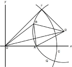
Figure 1: The fundamental triangle OAB with one side AB being an arc of the circle Q with center D. The orthogonal circle C is centered at the origin O and has the radius OF=$R$. DF and OF are perpendicular.

Recall from Section 4.1 that (4.3) maps the upper-half $s$-plane onto a circular triangle with two straight edges denoted by OA and OB as shown in Fig. 1. The third side of the triangle is formed by the circular arc AB which is part of the circle Q with center at D, and radius ${\rm AD}={\rm BD}:=r$. The vertices O, A, B correspond to the image points $z(0)=0$, $z(1)$ and $z(\infty)$ of the map (4.3), respectively. The angle $\pi\alpha=\angle{\rm BOA}$, while angles $\pi\beta$ and $\pi\gamma$ are the angles made by OA and OB respectively, with the circular arc AB. The orthogonal circle C is centered at the origin O and its radius OF:=$R$. Now consider the triangles OAB and DAB whose common side is given by the chord AB. From elementary considerations, it follows that $\angle{\rm ADB}=\pi-\pi(\alpha+\beta+\gamma)$, $\angle{\rm DAB}=\pi({\textstyle\frac{\alpha+\beta+\gamma}{2}})$, and $\angle{\rm OBA}={\textstyle\frac{\pi}{2}}-\pi({\textstyle\frac{\alpha+\beta-\gamma}{2}})$. Applying the law of sines to triangles OAB and DAB, and denoting ${\rm OA}=x$, one finds that

$$\mathrm{AB}=\frac{x\sin\pi\alpha}{\cos\pi({\textstyle\frac{\alpha+\beta-\gamma}{2}})},\qquad\mathrm{BD}:=r=\frac{\mathrm{AB}\sin\pi({\textstyle\frac{\alpha+\beta+\gamma}{2}})}{\sin\pi(\alpha+\beta+\gamma)}.$$

Eliminating AB from above, yields the following expression for the radius of the circle Q

$$r=\frac{x\sin\pi\alpha}{2\cos\pi({\textstyle\frac{\alpha+\beta-\gamma}{2}})\cos\pi({\textstyle\frac{\alpha+\beta+\gamma}{2}})}.$$ (B.1)

Since the circles Q and C are mutually orthogonal, their radii OF and DF are perpendicular. Hence from the right triangle ODF with hypotenuse ${\rm OD}=:d$ it follows that $R^{2}=d^{2}-r^{2}$. Next, considering the triangle OAD with $\angle{\rm OAD}={\textstyle\frac{\pi}{2}}+\pi\beta$, one obtains $d^{2}=x^{2}+r^{2}+2rx\sin\pi\beta$. Substituting this into the expression for $R^{2}$ and using (B.1), one obtains

$$R^{2}=x^{2}\frac{\sin{\textstyle\frac{\pi}{2}}(1-\alpha+\beta-\gamma)\sin{\textstyle\frac{\pi}{2}}(1-\alpha+\beta+\gamma)}{\sin{\textstyle\frac{\pi}{2}}(1-\alpha-\beta+\gamma)\sin{\textstyle\frac{\pi}{2}}(1-\alpha-\beta-\gamma)},$$ (B.2)

after using some trigonometric identities. From (4.3) the line segment OA$=x$ along the real axis is given by

$$x=z(1)=\frac{{}_{2}F_{1}(a-c+1,b-c+1;2-c;1)}{{}_{2}F_{1}(a,b;c;1)}=\frac{\Gamma(2-c)\Gamma(c-a)\Gamma(c-b)}{\Gamma(c)\Gamma(1-a)\Gamma(1-b)},$$

after using ${}_{2}F_{1}(a,b;c;1)=\Gamma(c)\Gamma(c-a-b)[\Gamma(c-a)\Gamma(c-b)]^{-1}$ [15]. Substituting the above expression for $x$ into (B.2), using the identity $\Gamma(t)\Gamma(1-t)=\pi\,\mathrm{csc}(\pi t)$, and replacing $(a,b,c)$ by their values in terms of $(\alpha,\beta,\gamma)$, one finally obtains the expression for $R^{2}$ in Section 4.1.

Acknowledgments

The work of SC was partly supported by NSF grant No. DMS-1410862. The work of OB was supported in part by a CRCW grant from University of Colorado, Colorado Springs. The authors thank Professor Mark Ablowitz for useful discussions, as well as the anonymous referees for their valuable remarks which substantially improved the article.

References

- [1] Ablowitz M.J., Chakravarty S., Halburd R., The generalized Chazy equation and Schwarzian triangle functions, Asian J. Math. 2 (1998), 619–624.
- [2] Ablowitz M.J., Chakravarty S., Halburd R., The generalized Chazy equation from the self-duality equations, Stud. Appl. Math. 103 (1999), 75–88.
- [3] Atiyah M., Hitchin N., The geometry and dynamics of magnetic monopoles, M.B. Porter Lectures, Princeton University Press, Princeton, NJ, 1988.
- [4] Bureau F.J., Integration of some nonlinear systems of ordinary differential equations, Ann. Mat. Pura Appl. 94 (1972), 345–359.
- [5] Chakravarty S., Differential equations for triangle groups, in Algebraic and Geometric Aspects of Integrable Systems and Random Matrices, Contemp. Math., Vol. 593, Amer. Math. Soc., Providence, RI, 2013, 179–204.
- [6] Chakravarty S., Ablowitz M.J., Integrability, monodromy evolving deformations, and self-dual Bianchi IX systems, Phys. Rev. Lett. 76 (1996), 857–860.
- [7] Chakravarty S., Ablowitz M.J., Parameterizations of the Chazy equation, Stud. Appl. Math. 124 (2010), 105–135, arXiv:0902.3468.
- [8] Chakravarty S., Ablowitz M.J., Clarkson P.A., Reductions of self-dual Yang–Mills fields and classical systems, Phys. Rev. Lett. 65 (1990), 1085–1087.
- [9] Chakravarty S., Ablowitz M.J., Takhtajan L.A., Self-dual Yang–Mills equation and new special functions in integrable systems, in Nonlinear Evolution Equations and Dynamical Systems (Baia Verde, 1991), World Sci. Publ., River Edge, NJ, 1992, 3–11.
- [10] Chazy J., Sur les équations différentielles du troisième ordre et d’ordre supérieur dont l’intégrale générale a ses points critiques fixes, Acta Math. 34 (1911), 317–385.
- [11] Clarkson P.A., Olver P.J., Symmetry and the Chazy equation, J. Differential Equations 124 (1996), 225–246.
- [12] Cosgrove C.M., Chazy classes IX–XI of third-order differential equations, Stud. Appl. Math. 104 (2000), 171–228.
- [13] Darboux G., Mémoire sur la théorie des coordonnées curvilignes, et des systèmes orthogonaux, Ann. Sci. École Norm. Sup. (2) 7 (1878), 101–150.
- [14] Dubrovin B., Geometry of D topological field theories, in Integrable Systems and Quantum Groups (Montecatini Terme, 1993), Lecture Notes in Math., Vol. 1620, Springer, Berlin, 1996, 120–348, hep-th/9407018.
- [15] Erdélyi A., Magnus W., Oberhettinger F., Tricomi F.G., Higher transcendental functions, Vol. 1, McGraw-Hill, 1953.
- [16] Ferapontov E.V., Galvão C.A.P., Mokhov O.I., Nutku Y., Bi-Hamiltonian structure of equations of associativity in -d topological field theory, Comm. Math. Phys. 186 (1997), 649–669.
- [17] Ford L.R., Automorphic functions, 2nd ed., Chelsea Publishing Co., New York, 1951.
- [18] Goursat E., Sur l’équation différentielle linéaire, qui admet pour intégrale la série hypergéométrique, Ann. Sci. École Norm. Sup. (2) 10 (1881), 3–142.
- [19] Halphen G., Sur une système d’équations différentielles,, C.R. Acad. Sci. Paris 92 (1881), 1101–1103.
- [20] Halphen G., Sur certains système d’équations différentielles, C.R. Acad. Sci. Paris 92 (1881), 1404–1407.
- [21] Hitchin N.J., Twistor spaces, Einstein metrics and isomonodromic deformations, J. Differential Geom. 42 (1995), 30–112.
- [22] Hitchin N.J., Hypercomplex manifolds and the space of framings, in The Geometric Universe (Oxford, 1996), Oxford Univ. Press, Oxford, 1998, 9–30.
- [23] Maier R.S., Nonlinear differential equations satisfied by certain classical modular forms, Manuscripta Math. 134 (2011), 1–42, arXiv:0807.1081.
- [24] Nehari Z., Conformal mapping, McGraw-Hill Book Co., Inc., New York, Toronto, London, 1952.
- [25] Ramanujan S., On certain arithmetical functions, Trans. Cambridge Philos. Soc. 22 (1916), 159–186.
- [26] Ramanujan S., Notebooks, Vols. 1, 2, Tata Institute of Fundamental Research, Bombay, 1957.
- [27] Ramanujan S., Collected Papers, Amer. Math. Soc., Providence, RI, 2000.
- [28] Randall M., Flat -distributions and Chazy’s equations, SIGMA 12 (2016), 029, 28 pages, arXiv:1506.02473.
- [29] Randall M., Schwarz triangle functions and duality for certain parameters of the generalised Chazy equation, arXiv:1607.04961.
- [30] Rosenhead L. (Editor), Laminar boundary layers, Clarendon Press, Oxford, 1963.
- [31] Schwarz H.A., Ueber diejenigen Fälle, in welchen die Gaussische hypergeometrische Reihe eine algebraische Function ihres vierten Elementes darstellt, J. Reine Angew. Math. 75 (1873), 292–335.
- [32] Vidūnas R., Algebraic transformations of Gauss hypergeometric functions, Funkcial. Ekvac. 52 (2009), 139–180, math.CA/0408269.