Application of Van Der Waals Density Functionals to Two Dimensional Systems Based on a Mixed Basis Approach

Abstract

A van der Waals (vdW) density functional was implemented in the mixed basis approach previously developed for studying two dimensional systems, in which the vdW interaction plays an important role. The basis functions here are taken to be the localized B-splines for the finite non-periodic dimension and plane waves for the two periodic directions. This approach will significantly reduce the size of the basis set, especially for large systems, and therefore is computationally efficient for the diagonalization of the Kohn-Sham Hamiltonian. We applied the present algorithm to calculate the binding energy for the two-layer graphene case and the results are consistent with data reported earlier. We also found that, due to the relatively weak vdW interaction, the charge density obtained self-consistently for the whole bi-layer graphene system is not significantly different from the simple addition of those for the two individual one-layer system, except when the interlayer separation is close enough that the strong electron-repulsion dominates. This finding suggests an efficient way to calculate the vdW interaction for large complex systems involving the Moiré pattern configurations.
PACS: 71.15.Mb, 73.20.-r

I INTRODUCTION

The electronic properties of two-dimensional (2D) systems are fundamentally different from those in higher dimensions due to their unusual collective excitations. Among these 2D materials, graphite is the most well known. Graphite has a layered planar structure and is electrically conductive along the planes, whereas diamond, another allotrope of carbon, is an insulator. Graphene is an isolated sheet of graphite and can be stacked via the weak van der Waals (vdW) interaction to form the graphite structure. There has been increasing interest in vdW graphene-based composite systems, e.g., alkali metal/graphite adsorption systems BKLW ; ZKSH or MoS2/graphene heterostructures PHABNP . Expectations concerning the creation of improved functional electrodevices with better performance characteristics are rising from the intensive exploration of such graphene-based materials.

First-principles methods based on the density functional theory within local density approximation (LDA) and generalized gradient approximation(GGA) have proven to be powerful and successful in investigating static and dynamic properties of materials with strong ionic, covalent and metallic interactions. Unfortunately, these methods fail to describe the weak vdW dispersion interaction properly. For example, GGA calculations show no relevant binding between graphite sheets RJHSLL . While the LDA approach predicts an underestimated minimum for graphite LM -NPA , it cannot capture the vdW physics ZKSH . Neither of these traditional functionals has basis to address issues of transferability for soft-matter problems involving the weak vdW bonding. To remedy this situation, a new approach using a van der Waals density functional (vdW-DF) with a nonlocal correlation energy has been developed by Dion et al DRSLL . This formalism accounts for the dominant dispersion energy, which is not correctly treated in standard DFT functionals.

In this work, we implement the vdW-DF functionals using the mixed basis approach developed previously RHC ; RCH . The basis functions here are taken to be the localized B-splines for the finite non-periodic dimension and 2D plane waves for the two periodic directions. B-splines are highly localized and piecewise polynomials deBoor , which have proven to be an excellent tool for the description of wavefunctions in a real-space approach RHC -RJH . Such a mixed-basis method LC ; LC1 avoids the use of artificial vacuum layers of large thickness introduced by the supercell modeling, reducing significantly the number of the basis functions, and therefore easing the computational burden for the diagonalization of the Kohn-Sham Hamiltonian. Another advantage of the present mixed basis method is that, for charged systems, the spurious Coulomb interaction between the defect, its images and the compensating background charge in the supercell approach can be automatically avoided. No further modification needs to be made in the total-energy calculation RCH .

We tested the present algorithm by studying the binding energy between two graphene sheets stacked in both AA and AB types, as depicted in Fig. 1. In addition, the charge density around each graphene sheet was found not to be significantly affected by the existence of another one, except when the two sheets are so close that the electron distributions of individual sheets overlap with each other and the strong electron repulsion dominates. This revelation would allow us to calculate the binding energy by the rigid-density model, i.e., the whole charge density for the system is simply the sum of those self-consistently calculated for the individual layers, instead of using the very time-consuming self-consistent density calculation for the whole system. The justified rigid-density model enables a simpler yet accurate evaluation of the vdW interaction for large complex systems including the Moiré pattern configurations. The results will be presented and discussed in details.

II METHOD OF CALCULATION

II.1 B-splines

For the sake of completeness, we first briefly summarize the B-spline formalism. More details can be found in Refs. RHC and deBoor . In general, B-spline of order $\kappa$ consists of positive polynomials of degree $\kappa-1$, over $\kappa$ adjacent intervals. These polynomials vanish everywhere outside the subintervals $\tau_{i}<z<\tau_{i+\kappa}$. The B-spline basis set of order $\kappa$ with the knot sequence $\{\tau_{i}\}$ is generated by the following relation :

$$B_{i,\kappa}(z)=\frac{z-\tau_{i}}{\tau_{i+\kappa-1}-\tau_{i}}B_{i,\kappa-1}(z)+\frac{\tau_{i+\kappa}-x}{\tau_{i+\kappa}-\tau_{i+1}}B_{i+1,\kappa-1}(z),$$ (1)

with

$$B_{i,1}(z)=\left\{\begin{array}[]{ll}1,&\tau_{i}\leq z<\tau_{i+1}\\ 0,&{\rm otherwise\ .}\end{array}\right.$$ (2)

The first derivative of the B-spline of order $\kappa$ is given by

$$\frac{d}{dz}B_{i,\kappa}(z)=\frac{\kappa-1}{\tau_{i+\kappa-1}-\tau_{i}}B_{i,\kappa-1}(z)-\frac{\kappa-1}{\tau_{i+\kappa}-\tau_{i+1}}B_{i+1,\kappa-1}(z).$$ (3)

Therefore, the derivative of B-splines of order $\kappa$ is simply a linear combination of B-splines of order $\kappa-1$, which is also a simple polynomial and is continuous across the knot sequence. Obviously, B-splines are flexible to accurately represent any localized function of $z$ with a modest number of the basis by only increasing the density of the knot sequence where it varies rapidly.

II.2 vdW-DF functional

The nonlocal energy functional proposed by Dion et al. DRSLL is

$$E^{vdW-DF}_{xc}=E^{revPBE}_{x}+E^{LDA}_{c}+E^{nl}_{c}.$$ (4)

The first two parts are simply revPBE exchange ZY and LDA correlation PW . $E^{nl}_{c}$ is a non-local correlation functional that was introduced to accounts for dispersion interactions, and is given as

$$E^{nl}_{c}=\frac{1}{2}\int\int{d{\bf r_{1}}d{\bf r_{2}}}n({\bf r_{1}})\phi(q_{1},q_{2},r_{12})n({\bf r_{2}}),$$ (5)

where $r_{12}=|\bf{r_{1}}-\bf{r_{2}}|$, and $q_{1},q_{2}$ are the values of a universal function $q_{0}$ at $\bf{r_{1}}$ and $\bf{r_{2}}$. It turns out that the kernel $\phi$ depends on $\bf{r_{1}}$ and $\bf{r_{2}}$ only through two variables $d_{1}=q_{1}r_{12}$ and $d_{2}=q_{2}r_{12}$, and can be expressed as

$$\phi(d_{1},d_{2})=\frac{2}{\pi^{2}}\int_{0}^{\infty}a^{2}da\int_{0}^{\infty}b^{2}db\ W(a,b)T(\nu(a),\nu(b),\nu^{{}^{\prime}}(a),\nu^{{}^{\prime}}(b)),$$ (6)

where $W$ and $T$ are defined as

$$W(a,b) = 2[(3-a^{2})b\cos b\sin a+(3-b^{2})a\cos a\sin b+$$ (7)

$$(a^{2}+b^{2}-3)\sin a\sin b-3ab\cos a\cos b]/a^{3}b^{3},$$

$$T(w,x,y,z) = \frac{1}{2}[\frac{1}{w+x}+\frac{1}{y+z}]\times[\frac{1}{(w+y)(x+z)}+\frac{1}{(w+z)(y+x)}].$$ (8)

The quantities $\nu$ and $\nu^{{}^{\prime}}$ are given by $\nu(u)=u^{2}/2h(u/d_{1})$ and $\nu^{{}^{\prime}}(u)=u^{2}/2h(u/d_{2})$ with $h(t)=1-\exp(-4\pi t^{2}/9)$.

The universal function $q_{0}$ reads as

$$q_{0}({\bf r})=-\frac{4\pi}{3}\epsilon_{xc}^{LDA}n({\bf r})-\frac{Z_{ab}}{9}s^{2}({\bf r})k_{F}({\bf r}).$$ (9)

Here, the Fermi wave vector $k_{F}$ and the reduced gradient $s$ are

$$k^{3}_{F}({\bf r})=3\pi^{2}n({\bf r}),\ s({\bf r})=\frac{\nabla n({\bf r})}{2k_{F}({\bf r})n({\bf r})},$$ (10)

and $Z_{ab}=-0.8491$.

The nonlocal correlation energy in Eq. (5) is expressed as a double spatial integral. To alleviate the $O(N^{2})$ evaluation of such the integral, we adopt the algorithm by Román-Pérez and Soler RS , which transforms the double real space integral to reciprocal space and reduces the computational effort.

First, $\phi$ was interpolated as

$$\phi(q_{1},q_{2},r_{12})=\sum_{\alpha,\beta}\phi(q_{\alpha},q_{\beta},r_{12})p_{\alpha}(q_{1})p_{\beta}(q_{2}),$$ (11)

where $q_{\alpha}$ are fixed values, chosen to ensure a good interpolation of function $\phi$. Here, we use cubic splines interpolation, in which $p_{\alpha}(q)$ is a succession of cubic polynomial in every interval $[q_{\beta},q_{\beta+1}]$, matching in value and the first two derivatives at every point $q_{\beta}$.

Substituting Eq. (11) into (5),

$$E^{nl}_{c}=\frac{1}{2}\sum_{\alpha,\beta}\int\int{d{\bf r_{1}}d{\bf r_{2}}}\theta_{\alpha}({\bf r_{1}})\theta_{\beta}({\bf r_{2}})\phi_{\alpha\beta}(r_{12}),$$ (12)

with $\theta_{\alpha}({\bf r})=n({\bf r})p_{\alpha}(q_{0}({\bf r}))$ and $\phi_{\alpha\beta}(r_{12})\equiv\phi(q_{\alpha},q_{\beta},r_{12})$. Now, with use of the convolution, just like the Coulomb energy, $E^{nl}_{c}$ becomes

$$E^{nl}_{c}=\frac{1}{2}\sum_{\alpha,\beta}\int{d{\bf k}}\theta_{\alpha}^{*}({\bf k})\theta_{\beta}({\bf k})\phi_{\alpha\beta}(k),$$ (13)

where $\theta_{\alpha}({\bf k})$ and $\phi_{\alpha\beta}(k)$ are the corresponding Fourier transforms. In practice, $\phi_{\alpha\beta}(k)$ was pre-calculated in spherical radial mesh of points $k$. Then, $\phi_{\alpha\beta}(k)$ and its second derivative via cubic spline interpolation were stored for later use. A logarithmic mesh of interpolation points $q_{\alpha}$, of which the total number is 20 in the present calculation, was used to describe $\phi$ up to a cutoff $q_{c}$ of 5.0 a.u..

II.3 GGA charge density in the mixed-basis approach

With one set of B-splines for the non-periodic $z$ direction and 2D plane waves for the periodic $xy$ plane, the present mixed basis used to expand the wavefuction is defined as

$$<{\bf r}|{\bf\ k_{\parallel}+G_{\parallel}};j,\kappa>\ =\frac{1}{\sqrt{A}}\ e^{i({\bf k_{\parallel}+G_{\parallel}})\cdot{\bf\rho}}\ B_{j,\kappa}(z),$$ (14)

where ${\bf G_{\parallel}}$ denotes an in-plane reciprocal lattice vector and ${\bf k_{\parallel}}$ is the in-plane Bloch wave vector. $A$ is the surface area of the system. Therefore, the charge density can be written in the form

$$n({\bf r})=\sum_{{\bf g}}\ n({\bf g},z)\ e^{i{\bf g}\cdot{\bf\rho}}\ ,$$

where ${\bf g}={\bf G_{\parallel}}-{\bf G^{{}^{\prime}}_{\parallel}}$.

Because the GGA energy functional depends upon $|\nabla n({\bf r})|$, the corresponding potential $v_{xc}$ is a functional of not only $|\nabla n|$, but also of $\nabla^{2}n$ and $\nabla n\cdot\nabla|\nabla n|$. In order to efficiently and precisely obtain $v_{xc}$, we used the method by White and Bird WB . First of all, we interpolate $n({\bf g},z)$ along the $z$ direction by using the Fourier interpolation technique:

$$n({\bf g},z)=\sum_{g_{z}}\ n({\bf g},g_{z})\ e^{ig_{z}z}\ .$$

Then,

$$n({\bf r})=\sum_{{\bf G}}n({\bf G})e^{i{\bf G}\cdot{\bf r}},$$ (15)

where ${\bf G}$ is a compact notation for $({\bf g},g_{z})$.

Following the procedure in Ref. WB ,

$$\nabla n({\bf r})=\sum_{{\bf G}}i{\bf G}n({\bf G})e^{i{\bf G}\cdot{\bf r}}=\frac{1}{N}\sum_{{\bf G,R}}i{\bf G}n({\bf R})e^{i{\bf G}\cdot({\bf r-R})}$$ (16)

$$=\frac{1}{N}\sum_{{\bf G}}i{\bf G}\left(\sum_{{\bf R}}n({\bf R})e^{-i{\bf G}\cdot{\bf R}}\right)e^{i{\bf G}\cdot{\bf r}},$$ (17)

with $N$ real space points ${\bf R}$ of the fast Fourier-transform (FFT) grid set.

We define $f_{xc}$ such that

$$E_{xc}[n]=\int f_{xc}(n({\bf r}),|\nabla n({\bf r})|)d{\bf r}.$$ (18)

$E_{xc}[n]$ can be approximated by

$$E_{xc}[n]\approx\frac{V}{N}\sum_{{\bf R}}f_{xc}(n({\bf R}),|\nabla n({\bf R})|).$$ (19)

The associated xc potential at the FFT grid point R can be obtained efficiently through

$$v_{xc}({\bf R}) = \frac{N}{V}\frac{dE_{xc}}{dn({\bf R})}$$ (20)

$$= \frac{\partial f_{xc}}{\partial n({\bf R})}+\sum_{{\bf R^{{}^{\prime}}}}\frac{\partial f_{xc}}{\partial\nabla n({\bf R^{{}^{\prime}}})}\cdot\frac{d\nabla n({\bf R^{{}^{\prime}}})}{dn({\bf R})}$$ (21)

$$= \frac{\partial f_{xc}}{\partial n({\bf R})}+\frac{1}{N}\sum_{{\bf G,R^{{}^{\prime}}}}i{\bf G}\cdot\frac{\partial f_{xc}}{\partial\nabla n({\bf R^{{}^{\prime}}})}e^{i{\bf G}\cdot({\bf R^{{}^{\prime}}-R})}$$ (22)

$$= \frac{\partial f_{xc}}{\partial n({\bf R})}+\frac{1}{N}\sum_{{\bf G,R^{{}^{\prime}}}}i{\bf G}\cdot\frac{\nabla n({\bf R^{{}^{\prime}}})}{n({\bf R^{{}^{\prime}}})}\frac{\partial f_{xc}}{\partial|\nabla n({\bf R^{{}^{\prime}}})|}e^{i{\bf G}\cdot({\bf R^{{}^{\prime}}-R})}.$$ (23)

Given the charge density on the FFT grid points, only eight FFT’s are required to obtain $v_{xc}$. That is computationally moderate with respect to the derivation of the second derivative needed to evaluate the conventional potential via

$$v_{xc}({\bf r})=\frac{\partial f_{xc}}{\partial n({\bf r})}-\nabla\cdot\frac{\partial f_{xc}}{\partial\nabla n({\bf r})}.$$ (24)

II.4 vdW-DF total energy

For the vdW-DF total energy functional, we first performed the self-consistent total energy calculation using the GGA-PBE functional PBE . With the converged charge density obtained in the previous step, the revPBE exchange energy ZY and LDA correlation energy PW are evaluated and substituted for the GGA-PBE counterparts, and the nonlocal correlation energy $E^{nl}_{c}$ is added. Now, the vdW-DF energy functional is written

$$E^{vdW-DF}=E^{PBE}-E^{PBE}_{xc}+(E^{revPBE}_{x}+E^{LDA}_{c}+E^{nl}_{c}).$$ (25)

The last three terms in the above equation are treated as a post-GGA perturbation because of their low sensitivity to the choice of GGA electronic density. By the present approach, $E^{nl}_{c}$ was obtained via

$$E^{nl}_{c}=\frac{1}{2}A\sum_{\alpha,\beta}\sum_{\bf g}\int{d{k_{z}}}\theta_{\alpha}^{*}({\bf k})\theta_{\beta}({\bf k})\phi_{\alpha\beta}(k),$$ (26)

with ${\bf k}=({\bf g},k_{z})$.

The interplanar binding energy per surface atom $E_{b}$ is defined as

$$E_{b}=(E_{bilayer}-2E_{graphene})/N_{b}$$ (27)

where $E_{bilayer}$ and $E_{graphene}$ are respectively the total energy of the bilayer graphene system and that of the system containing only one graphene sheet. $N_{b}$ is the number of atoms in one single graphene sheet.

III APPLICATIONS OF PRESENT METHOD

To test the present approach, we apply it to investigate the vdW interaction between graphene sheets. The calculations were carried out with the unit cell containing two graphene sheets. Here, we study both AA and AB stacking, as depicted in Fig. 1. In the former case, the carbon atoms of the adjacent sheets are aligned directly on top of each other. In the latter case, the energetically more stable structure, the graphene layers are shifted relative to each other such that half of the atoms are located exactly over the center of a hexagon and another half lie directly on top of the atoms in the second graphene sheet.

All C atoms in the graphene sheet were kept at the ideal positions. The in-plane lattice constant $a_{0}$ was fixed to the experimental value of 2.461 Å, while the inter-plane distance $d$ is allowed to vary. A FFT mesh with the grid spacing of 0.08 Å for the charge density are chosen for accurate total energy calculations. A mixed basis set with 34 B-splines distributed over a maximum range of 6.0 $a_{0}$ and 2D plane waves with an energy cutoff of 30 Ry are used to expand the wavefunction. The $7\times 7$ Monkhorst-Pack grids including $\Gamma$ point were taken to sample the surface Brillouin zone. We used the Vanderbilt’s ultra-soft pseudopotential (USPP) DV . The C USPP was generated from the Vanderbilt’s code vancode and its quality was examined previously RHC . The potential is determined self-consistently until its change is less than $10^{-7}$ Ry. Finally, the vdW-DF total energy and the associated binding energy are calculated according to the procedure described in Sec. II.4. For comparison, we also performed calculations by using the standard supercell approach implemented in the popular VASP code with the projector-augmented-wave potential (PAW) KJ ; KF . A typical vacuum space of 10 Å  required in VASP was used in the calculation.

The binding energy of bilayer graphene in the AA stacking as a function of interlayer separation $d$ is shown in Fig. 2. The VASP counterpart is also plotted for comparison. Obviously, the GGA-PBE calculations show no relevant minimum for the graphite binding energy, reflecting the failure to include the proper long-range dispersive interaction within the GGA approximation. On the other hand, with the vdW-DF xc functional expressed in Eq. (4), we obtained for the graphene pair a binding energy of 47 meV/atom for the AA stacking. More importantly, the results obtained with our algorithm agree nicely with those by the popular VASP code. We are then convinced that the present program has been implemented successfully for the vdW interaction and the outcomes are very reliable.

We also calculated for the AB stacking and the resulting binding energy is displayed in Fig. 3. Clearly, the AB stacking is energetically more stable than the AA stacking, in agreement with the experiment that natural graphite occurs mainly with AB stacking order THZ . The binding energy for the AB stacking was found to be 50.5 meV/atom at the distance of 3.7 Å  and that for the less favored AA stacking was 47.0 meV/atom at the distance of 3.8 Å. The results are consistent with data reported in the literature NPA ,CSLL -CKHS . It can be seen from this figure that the $E_{b}$ curve for the AB stacking merges into that for the AA stacking at large separation $d$, which seemingly indicates that the total energy will be less sensitive to the orientation of the two graphene sheets if the separation is not too close.

Actually, contrary to the covalent bond, the charge density distribution near the individual graphene sheet would not be noticeably affected via the weak vdW interaction from other sheets unless the sheet separation is close enough such that it begins to ’contact’ or even overlaps with the density from the adjacent sheet. In that case, the shape of the density distribution around the graphene sheet will be distorted because of the dominant strong electron repulsion.

To justify this assertion, we use a rigid-density model, i.e., the whole charge density of the system in the AA stacking is simply assumed to be the sum of those self-consistently calculated for the individual single layer. Then we employed such charge density to re-calculated the total energy $E^{tot,AA}_{rigid}$ and compared it to the total energy $E^{tot,AA}_{scf}$ with self-consistent density calculations. The results are summarized in Table 1. Here, we chose seven cases with various interlayer separation $d$, as also indicated in Fig. 3. Clearly, the total energy per surface atom by the rigid-density model is very similar to the self-consistent total energy. The energy difference only becomes notable (2.7 meV/atom) for Case 7 with $d=2.95$ Å, which already enters the electron-repulsive region. With detailed analysis of energy components, we found that even though the energy difference from the kinetic energy part is somewhat sizable (for example, 32 meV/atom for Case 4 with $d=3.69$ Å), but it is largely compensated for with the Hartree energy part, leading to almost the same value in total.

When the charge density of the single graphene sheet was shifted a bit to the second one, we obtained similar conclusion, as shown in Table 1 for the AB stacking. Therefore, it is reasonable to expect that if the first graphene sheet is rotated with respect to the second to become a Moiré rotated pattern, the rigid-density model can still hold to efficiently predict a reliable binding energy for such a large complex system. This finding is promising in searching for the true ground-state atomic configuration for vdW-dominated graphene-based materials, like MoS2/graphene heterostructures PHABNP . Instead of using the very time-consuming self-consistent approach for such materials, the rigid-density model allows us to only focus on accurate charge density calculations of every individual slab of different type.

IV CONCLUSIONS

In conclusion, we have successfully implemented the van der Waals (vdW) density functional proposed by Dion et al. DRSLL in our mixed-basis approach for investigating the bi-layer graphene system. As compared to the conventional supercell model with alternating slab and vacuum regions, it is a real space approach along the non-periodic direction. Therefore, the number of the basis functions used to expand the wavefunction is significantly reduced, especially for large complex systems.

We also found that the self-consistent total energy obtained for the bilayer system is not significantly different from that with charge density assumed to be the simple sum of those for the two individual single-layer system, except when the distance between the two layers is close enough that the strong electron-repulsion dominates. Such observations help us to propose a rigid-density model which can efficiently calculate the binding of vdW-dominated 2D systems with Moiré pattern configurations.

*

Appendix A

Fig. 1: Atomic structure of the graphite in both AA and AB stacking.

Fig. 2: (Color online) Binding energy for the two-layer graphenes in AA stacking calculated with GGA-PBE and vdW-DF xc functionals. The counterparts obtained by VASP are also displayed for comparison.

Fig. 3: (Color online) Binding energy for the two-layer graphenes in both AA and AB stacking calculated with vdW-DF xc functional.

Figure 1:

Figure 2:

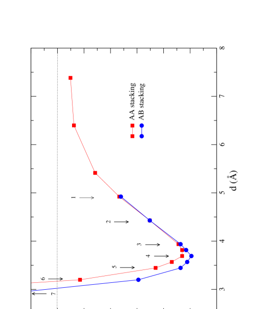
Figure 3:

Table 1: Total energy difference per surface atom between those obtained by the self-consistent calculation and rigid-density model for the bilayer graphene system with various interlayer separation $d$ in both AA and AB stacking. See text for details.

case No.	$d$	$E^{tot,AA}_{scf}-E^{tot,AA}_{rigid}$	$E^{tot,AB}_{scf}-E^{tot,AB}_{rigid}$
	(Å)	(meV/atom)	(meV/atom)
1	4.92	0.2	0.1
2	4.43	-0.1	-0.1
3	3.94	0.2	-0.3
4	3.69	0.1	0.2
5	3.45	-0.4	0.2
6	3.20	0.7	0.4
7	2.95	2.7	1.1

References

- (1) M. Breitholtz, T. Kihlgren, S. -Å. Lindgren, and L. Walldén, Phys. Rev. B 66, 153401 (2002).
- (2) E. Ziambaras, J. Kleis, E. Schröder, P. Hyldgaard, Phys. Rev. B 76, 155425 (2007).
- (3) D. Pierucci,H. Henck, J. Avila, A. Balan, C. H. Naylor, G. Patriarche, Y. J. Dappe, M. G. Silly, F. Sirotti, A. T. C. Johnson, M. C. Asensio, and A. Ouerghi, Nano Lett. 16, 4054 (2016).
- (4) H. Rydberg, N. Jacobson, P. Hyldgaard, S. I. Simak, B. I. Lundqvist, and D. C. Langreth, Surf. Sci. 532-535, 606 (2003).
- (5) I. -H. Lee and R. M. Martin, Phys. Rev. B 56, 7197 (1997).
- (6) J. C. Boettger, Phys. Rev. B 55, 11202 (1997).
- (7) D. Nabok, P. Puschnig, and C. Ambrosch-Draxl, Comp. Phys. Comm. 182, 1657 (2011).
- (8) M. Dion, H. Rydberg, E. Schröder, D. C. Langreth, and B. I. Lundqvist, Phys. Rev. Lett. 92, 246401 (2004), 95, 109902(E) (2005).
- (9) C. Y. Ren, C. S. Hsue and Y.-C. Chang, Comp. Phys. Comm. 188, 94 (2015).
- (10) C. Y. Ren, Y.-C. Chang, and C. S. Hsue, Comp. Phys. Comm. 202, 188 (2016).
- (11) Carl deBoor, A practical Guide to Splines, (Springer, New York, 1987).
- (12) W. R. Johnson, S. A. Blundell, and J. Sapirstein, Phys. Rev. A 37, 307 (1988).
- (13) H. T. Jeng, and C. S. Hsue, Phys. Rev. B 62, 9876 (2000).
- (14) C. Y. Ren, H. T. Jeng, and C. S. Hsue, Phys. Rev. B 66, 125105 (2002).
- (15) G.-W. Li and Y.-C. Chang, Phys. Rev. B 48, 12032 (1993).
- (16) G.-W. Li and Y.-C. Chang, Phys. Rev. B 50, 8675 (1994).
- (17) Y. Zhang and W. Yang, Phys. Rev. Lett. 80, 890 (1998).
- (18) J. P. Perdew and Y. Wang, Phys. Rev. B 45, 13244 (1992) and references therein.
- (19) G. Román-Pérez, and J. M. Soler, Phys. Rev. Lett. 103, 096102 (2009).
- (20) J. A. White and D. M. Bird, Phys. Rev. B 50, 4954(R) (1994).
- (21) J. P. Perdew, K. Burke, and M. Ernzerhof, Phys. Rev. Lett. 77, 3865 (1996).
- (22) D. Vanderbilt, Phys. Rev. B 41, 7982 (1990).
- (23) http://www.physics.rutgers.edu/ dhv/uspp/.
- (24) G. Kresse and D. Joubert, Phys. Rev. B 59, 1758 (1999).
- (25) G. Kresse and J. Furthmüller, Comput. Mater. Sci. 6, 15 (1996).
- (26) P. H. Tan, W. P. Han, W. J. Zhao, Z. H. Wu, K. Chang, H. Wang, Y. F. Wang, N. Bonini, N. Marzari, N. Pugno, G. Savini, A. Lombardo, A. C. Ferrari, Nat. Mater. 11, 294 (2012).
- (27) S. D. Chakarova-Käck, E. Schröder, B.I. Lundqvist, and D.C. Langreth, Phys. Rev. Lett. 96, 146107 (2006).
- (28) S. D. Chakarova-Käck, J. Kleis, P. Hyldgaard, and E. Schröder, New J. Phys. 12, 013017 (2010).
FIGURE CAPTIONS