Dynamically enhanced optical coherence tomography

Abstract

In the investigations of inhomogeneous media, availability of methods to study the interior of the material without affecting it is valuable. Optical coherence tomography provides such a functionality, by providing depth resolved images of semi-transparent objects non-invasively. This is especially useful in medicine, and is used not only in research, but also in clinical practice. Optical coherence tomography characterizes each cross-section by its reflectance. It is clearly desirable to obtain more detailed information regarding each cross-section, if available. We have developed a system which measures the fluctuation spectrum of all the cross-sections in optical coherence tomography. By providing more information for each cross-section, this can in principle be effective in tissue characterization and pathological diagnosis. The system uses the time dependence of the optical coherence tomography data, to obtain the fluctuation spectrum of each cross-section. Additionally, noise reduction is applied to obtain the spectra without unwanted noise, such as shot-noise, which can swamp the signal. The measurement system is applied to samples with no external stimuli, and depth resolved thermal fluctuation spectra of the samples are obtained. These spectra are compared with their corresponding theoretical expectations, and are found to agree. The measurement system requires dualizing the detectors in the optical coherence tomography, but otherwise requires little additional equipment. The measurements were performed in ten to a hundred seconds.

I Introduction

Optical coherence tomography (OCT)oct1 ; oct2 uses low-coherence reflectometry to obtain cross-sectional images of inhomogeneous media, such as biological tissue. OCT is particularly useful in the biomedical area, since the imaging can be performed non-invasively, and in a relatively short time. As such, OCT is not only used in research, but has proven to be effective in clinical practice, with the fields of its application continuing to growoctReview1 . In OCT, essentially, the reflectance of each cross-section along the depth direction is obtained with high spatial resolution (${\sim 10\,\mu}$m), revealing the structure of the sample.

In implementing OCT, two main approaches exist, referred to as time-domain OCT (TD-OCT)oct1 ; oct2 and Fourier-domain OCT (FD-OCT)sdoct1 ; sdoct2 . OCT makes use of interferometry, and TD-OCT resolves the depth by effectively moving the reference (or the sample) in the interferometry, while FD-OCT spectrographically resolves the depth information. FD-OCT has an advantage that the OCT image can be obtained with a single exposure, with the sensitivity a few hundred times better than that of TD-OCT, but gives rise to virtual images unless further processing is performed. The relative merits of the two approaches were analyzed, and a method for removing virtual images has been found Mitsui99 ; Leitgeb2003 ; Boer2003 . OCT essentially measures the reflectance of each cross-section, and this can lead to information regarding the matter buried beneath the surface, when the material is semi-transparent. Results from OCT can also be combined with Doppler velocimetry, and has been applied to angiographyoctDoppler ; octReview1 ; octDoppler2 ; octDopplerReview . It is clearly desirable to obtain more information, in addition to its reflectance, regarding each cross-section in OCT.

In this work, we have developed a system that combines OCT with thermal fluctuation measurements, which extracts physical properties, such as the viscoelastic characteristics, of each cross-section in the depth direction. We demonstrate the efficacy of this system using various samples. Furthermore, the noise is reduced to below shot-noise levels using averaged correlations, making it possible to extract spectral information otherwise unobtainable. The measurement system can in principle lead to tissue characterization and pathological diagnosis.

II The theory underlying dynamically enhanced optical coherence tomography

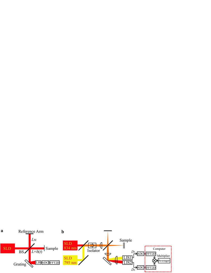
Figure 1: Experimental setup for the dynamically enhanced OCT system: a, The basic conceptual setup of the measurement system: Light from a superluminescent light diode (SLD), is fed into a Michelson interferometer with a reference arm, and a sample. The light from the interferometer is spectrally decomposed by a grating, and its intensity is measured for each wavelength by a linear imaging sensor (LIS). The photocurrent from LIS is digitized by an analog-to-digital converter (ADC), and Fourier transformed both in $k$, and $t$ (FFT2D), to obtain the power spectra of all the cross-sections in OCT. BS: beam splitter. b, The schematics of the measurement system used in this work: The basic concept in a is dualized with light sources with central wavelengths 795, 834 nm, for noise reduction to observe at sub-shot-noise levels. Noise reduction is achieved by computing the averaged correlation of the two measurements (Averager). The light powers at the sample were 36 $\mu$W, 50 $\mu$W, for the two wavelengths, respectively.

In this work, we measure the time dependence of the FD-OCT signal to obtain the thermal fluctuation spectra of each cross-section in OCT. Measuring thermal fluctuation spectra of surfaces and interfaces has proven to be effective in extracting the physical properties of the material, such as viscoelastic characteristicsripplonExp ; Cicuta2004 ; Sagis . The basic concept underlying the measurement system is as follows: Consider a Michelson interferometer with a reference arm, and a sample with reflectance $R$, (Fig. 1a). For the light with a particular wave number $k$, and angular frequency $\omega_{\rm L}$, the detected light power, $P(k,t)$, from the interferometer is

$$P(k,t)=A\left|e^{i2kL_{\rm M}-i\omega_{\rm L}t}+Re^{i2k(L+\delta(t))-i\omega_{\rm L}t}\right|^{2}=A\left[1+R^{2}+2R\cos 2k(\Delta L+\delta(t))\right]\quad,$$ (1)

where $L_{M},L$ are the arm lengths of the interferometer to the mirror, sample surface respectively, $\Delta L=L-L_{\rm M}$, and $A$ is a constant. $\delta(t)$ is the fluctuation of the sample surface location in the light direction, defined such that its average is zero. By Fourier transforming $P(k,t)$ both in $k$, and in $t$, the power spectra of the fluctuations $S(\Delta L,f)$ for a given $\Delta L$ is obtained, so that all the cross-sections are computed simultaneously.

In practice, the Fourier transform in $k$ is performed within a finite region, determined by the spectral width of the incoming light. This gives rise to a form factor that selects the location of the cross-section, $\Delta L$. Assuming a Gaussian spectrum for $k$, we obtain $Q(x,\omega)$, the Fourier transform of $P(k,t)$ both in $k$ and $t$,

$$Q(x,\omega)=\int_{-\infty}^{\infty}dt\,e^{i\omega t}\int_{-\infty}^{\infty}{dk\over 2\pi}\,{e^{-(k-k_{0})^{2}/(2\sigma_{k}^{2})}\over\sqrt{2\pi}\sigma_{k}}e^{ikx}P(k,t)\quad.$$ (2)

Here, $\sigma_{k}$ is the standard deviation of the spectral distribution, and $\omega=2\pi f$. Since we are interested in time-dependent ($\omega\not=0$) fluctuations, time independent terms will be suppressed in the equations. It should be noted that only $\delta$ is time-dependent in $P(k,t)$. The power spectrum of the fluctuations at $x$ is $|Q(x,\omega)|^{2}$, up to a constant.

Using $P(k,t)$ in Eq. (1), the integration over $k$ can be performed to obtain

$$Q(x,\omega)={AR\over 2\pi}\int_{-\infty}^{\infty}dt\,e^{i\omega t}\left[e^{-\sigma_{k}^{2}(x-2\Delta L-2\delta)^{2}/2+ik_{0}(x-2\Delta L-2\delta)}+e^{-\sigma_{k}^{2}(x+2\Delta L+2\delta)^{2}/2+ik_{0}(x+2\Delta L+2\delta)}\right]$$ (3)

In this work, we shall concentrate on thermal fluctuations, which are at the atomic scale, so that $k_{0}\delta\ll 1$. Keeping the leading terms in $\delta$, and we find

$$Q_{+}(x,\omega)={AR\over\pi}e^{-\sigma_{k}^{2}(x-2\Delta L)^{2}/2}\left[ik_{0}+\sigma_{k}^{2}(x-2\Delta L)\right]\tilde{\delta}(\omega)\quad,$$ (4)

where tilde denotes the Fourier transform in $t$. We have selected the term peaked in $x$ at $2\Delta L$ as $Q_{+}$. Another term exists with $\Delta L\rightarrow-\Delta L$. The power spectrum is obtained essentially by squaring the above quantity,

$$\left|Q_{+}(x,\omega)\right|^{2}=\left({AR\over\pi}\right)^{2}e^{-\sigma_{k}^{2}(x-2\Delta L)^{2}}\left[k_{0}^{2}+\sigma_{k}^{4}(x-2\Delta L)^{2}\right]\left|\tilde{\delta}(\omega)\right|^{2}$$ (5)

So the doubly Fourier transformed power spectrum of $P(k,t)$ leads to a thermal power fluctuation spectrum for each depth, $x/2$. Of the two terms in the square brackets in the above expression, the first term is dominant unless the spectrum is broad. The Gaussian prefactor is similar to that in the standard OCTSwanson92 ; sdoct1 ; octReview1 , except that it is squared in the power spectrum used here.

When the above procedure is applied to measuring the spectrum of fluctuations inside a medium, two main additional points need to be considered. First, $\Delta L$ is the optical length. Second, fluctuations from the medium in front of the measured location contributes to the spectrum, in general, as we now explain. Let the cross-section under consideration be at a depth $d$ in an uniform medium with an index of refraction, $n$. Assume that the surface of this medium is at distance $L^{\prime}$ from the beam splitter, and has fluctuation $\delta^{\prime}(t)$ in the beam direction. The light power from the interferometer is,

$$P^{\prime}(k,t)=A\left|e^{i2kL_{\rm M}-i\omega t}+Re^{i2k(L^{\prime}+\delta^{\prime})+i2nk(d+\delta-\delta^{\prime})-i\omega t}\right|^{2}\quad.$$ (6)

Comparing this with the simple interferometer power, Eq. (1), one can see that the effect is to replace $L$ by the optical length, $L^{\prime}+nd$, and to replace $\delta$ by $n[\delta+(1-n)/n\times\delta^{\prime}]$. The fluctuation $\delta^{\prime}$ affects the spectrum by changing the optical path length to the location of interest. As such, only the fluctuations in the light path where the index of refraction changes, or at partially reflecting surfaces, contribute to the spectrum. Also, it should be noted that the fluctuations $\delta$ is enhanced by $n$, while $\delta^{\prime}$ is suppressed relatively by $(1-n)/n$. $\delta,\delta^{\prime}$ are independent and the contribution to the spectrum will be proportional to $|\tilde{\delta}|^{2}+(n-1)^{2}/n^{2}{|\tilde{\delta}^{\prime}|^{2}}$. These fluctuations in the light path occur only at partially reflective interfaces, and are included in the dynamically enhanced OCT data for the smaller depth, so that they can be deconvoluted, in theory.

In the current experiment, the height fluctuation power spectrum from the Michelson interferometry, Eq. (1), is obtained. However, the measured light powers $P_{1,2}$ at the two linear image sensors in the setup Fig. 1b contain both the desired signal, $X$, along with the unwanted noise $N_{1,2}$, as $P_{j}=X+N_{j}\ (j=1,2)$. This noise unavoidably contains the shot-noise, which is due to the quantum nature of light, along with other experimental noise. We now briefly explain how the noise reduction is applied is to obtain the spectrum. The power spectrum of a signal, $X$, is obtained as

$${S}(f)=\int_{-\infty}^{\infty}\!\!d\tau\,e^{-i2\pi f\tau}\langle X(t)X(t+\tau)\rangle={1\over{\cal T}}\langle\left|\tilde{X}(2\pi f)\right|^{2}\rangle\quad,$$ (7)

where $\langle\cdots\rangle$ denotes averaging, $f$ is the frequency, and $\cal T$ is the measurement time. In the experiment, the noise was reduced statistically as followsMA1 : Let us assume that $N_{j}$ are uncorrelated between the two sensors. Then,

$$\langle\overline{\tilde{P}_{1}}\tilde{P}_{2}\rangle\longrightarrow\langle|\tilde{X}|^{2}\rangle\qquad({\cal N}\rightarrow\infty)\quad,$$ (8)

where $\cal N$ is the number of averagings. Shot-noise is a typical example of such uncorrelated noise, and it should be noted that this averaging procedure also reduces any other extraneous noise that is uncorrelated in the two photocurrents. This reduction is statistical, so the residual noise is $1/\sqrt{\cal N}$, relatively.

To understand the observed thermal fluctuation spectrum of each cross-section in the dynamically enhanced OCT, the corresponding theoretical spectrum needs to be understood. The obtained measurement, Eq. (5), is the height fluctuation power spectra for each depth, up to constants. The height fluctuation spectrum measured using Michelson interferometry is, theoreticallyMA2 ,

$${S_{\rm h}}(f)=2\int_{k_{\rm min}}^{\infty}dk\,ke^{-w^{2}k^{2}/4}F(k,\omega)$$ (9)

where $F(k,\omega)$ is the spectral function, $w$ is the beam waist, and $k_{\rm min}$ is determined by the physical size of the sample. For the results obtained below, we need the thermal fluctuations of a liquid surface, whose spectral function isLevich ; Bouchiat ; ripplonExp

$$F(k,\omega)={k_{\scriptscriptstyle\rm B}T\over 4\pi}{\rho\over\eta^{2}k^{3}\omega}{\rm\,Im}\left[(1+s)^{2}+y-\sqrt{1+2s}\right]^{-1},\quad s=-i{\rho\omega\over 2\eta k^{2}}\quad y={\sigma\rho\over 4\eta^{2}k},\quad.$$ (10)

Here, $\rho,\sigma,\eta$ are the density, the surface tension and the viscosity of the fluid. The above theoretical considerations, physical properties of the fluid, and the beam waist determine the theoretical fluctuation spectra completely.

III Experimental setup

The basic concept of the measurement system, shown in Fig. 1a, is as follows: The sample and the reference constitute the arms of a Michelson interferometer, which uses the light from a superluminescent light diode, a low-coherence light source. The spectrum of the interference signal light is obtained by using a grating, and a linear imaging sensor (LIS). This realizes the FD-OCT measurement system. We further measure the time dependence of the fluctuations of the light intensity, and use this to obtain the power spectra of all the cross-sections in the depth direction, individually. The thermal fluctuations are at atomic scales, and shot-noise, which inevitably arises due to the quantum nature of light, can contribute significantly to their spectra. To overcome this problem, the setup (Fig. 1b) incorporates noise reduction, whose theory was explained in the previous section. This is achieved statistically by dualizing the light source and their corresponding reflection measurements, then averaging the correlation of the light powers measured at LIS’sMA1 .

The technical details of the experimental setup are now explained: In the setup, Fig. 1, superluminescent diodes, QSDM-790-9, and QSDM-830-9 (both QPhotonics, USA), with central wavelengths 795 nm, and 834 nm and spectral widths 43 nm, and 24 nm, respectively, were used as light sources. This leads to a depth resolution of $9\,\mu$moctReview1 . The objective lens used to focus the light onto the sample had a numerical aperture of 0.015, and the beam waist at the sample was at the diffraction limit, 20 $\mu$m. Light powers were 36, 50 $\mu$W at the sample, for the two aforementioned light sources, respectively. For reflected light power measurement, linear image sensors, S12198-512Q (Hamamatsu, Japan) were used. 14 bit analog-to-digital converters, ADXII-14 (Saya, Japan) were used to digitize the photocurrent. Fourier transforms and averagings were performed on a computer. The clock for the linear image sensor is 10 MHz, and 1024 cycles are necessary for one readout, and 1024 lines were measured in a time series. Therefore, one measurement requires $0.1\,$s. Typically a few hundred to a thousand measurements were taken for the averaging, so the time required is $100\,$s or less.

IV Observations of depth resolved thermal fluctuation spectra

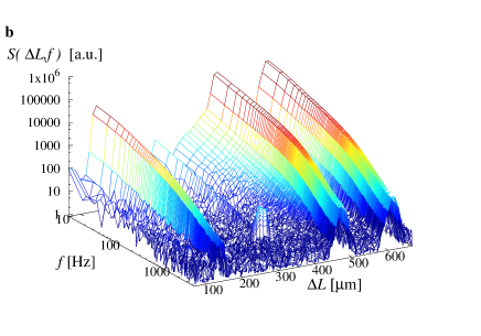
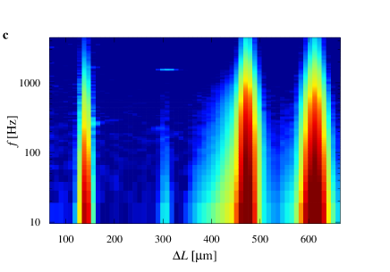
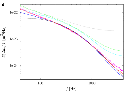
Figure 2: Dynamically enhanced OCT measurements of an oil film: a, Oil is suspended perpendicularly to the light direction in a circular hole with diameter $0.50\,$mm, thickness $0.10\,$mm. b,c, The thermal fluctuations of each cross-section along the light beam and the contour plot. $f$: frequency. d, The thermal fluctuation spectra of the two strongly reflective cross-sections at $\Delta L=470\,\mu$m (red), 613 $\mu$m (blue), and the third reflective cross-section at $\Delta L=143\,\mu$m (magenta). These measured spectra all have essentially the same shape, and their theoretical prediction is shown as the black line, which agrees with the measurements quite well. The spectra without the statistical noise reduction are also shown for the three cross-sections, which includes the shot-noise (cyan, green, gray lines, respectively). The noise is relatively larger for smaller reflected power, and the observed shot-noise levels are consistent with theory.

In Fig. 2b,c, the thermal fluctuation spectra for the cross-sections of an oil film suspended in a hole are shown. The configuration of the experiment is shown in Fig. 2a, and oil refers to silicone oil, Shin-Etsu KF96 300csShinetsu , with index of refraction 1.40, here, and below. Two strongly reflecting cross-sections centered at $\Delta L=475,\ 618\,\mu$m can be seen, with another signal peak at $\Delta L=143\,\mu$m. The first two cross-sections correspond to the two oil interfaces with air. The thickness 0.10 mm agrees with its optical depth, 0.14 mm, the difference between the two values of $\Delta L$. The signal peak at $\Delta L=143\,\mu$m is caused by the interference between the two cross-sections, and $\Delta L$ is the optical depth of the film. The thermal fluctuation spectra of these three cross-sections should all correspond to that of the height fluctuations of the oil surface, and they are essentially identical, as seen in Fig. 2d. Using known physical properties of the oil, the corresponding theoretical spectrum can be computed which is seen to agree quite well with the measured spectra. The physical properties of oil $(\rho\,{\rm[kg/m^{3}]},\sigma\,{\rm[kg/s^{2}]},\eta\,{\rm[kg/(m\cdot s)]})=(970,0.0211,0.291),(997,0.072,8.99\times 10^{-4})$, with the experimental temperature of 25${}^{\circ}\,{\rm C}$, were used here, and below. In the spectrum, $k_{\rm min}=\pi/(100\,\mu$m) was used, considering the thickness of the oil film. There is a normalization factor for each measured spectrum, which was chosen to match the overall magnitude of the theoretical spectrum. In Fig. 2d, the fluctuation spectra with noise reduction are $\langle\overline{\tilde{P}_{1}}\tilde{P}_{2}\rangle$, and the spectra without it are $\langle\overline{|\tilde{P}_{j}}|^{2}\rangle\ (j=1,2)$, in the notations of the previous section, with the same normalizations. The statistical noise reduction can be seen to be important for obtaining the precise spectrum. While the shot-noise can also be reduced relatively by increasing the light power, this will lead to invasive measurements in general.

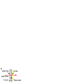
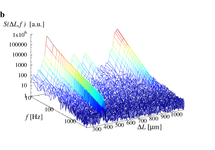
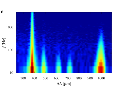
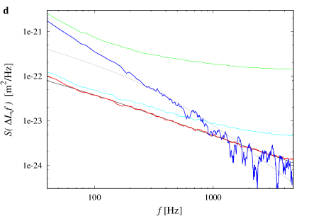
Figure 3: Dynamically enhanced OCT measurements of water and oil film fluctuations: a, Configuration: water, and oil films are perpendicular to the light direction, and are separated by a glass plate (thickness 0.16 mm). b,c, Thermal fluctuations of each cross-section in OCT, and the contour plot. d, The thermal fluctuation spectra for the two most reflective cross-sections in b,c, at $\Delta L=380\,\mu$m (red), and 998$\,\mu$m (blue). The theoretical spectra for water (black), oil (gray) are also shown and are consistent with the measurements. The spectra without the statistical noise reduction are also shown for the two cross-sections (cyan, green, respectively).

In Fig. 3b,c, the measured thermal spectra of the cross-sections of oil and water films, separated by a glass plate are shown (configuration in Fig. 3a). The structure of the fluctuation spectra of the cross-sections, whose reflective peaks are shown in Fig. 3b,c is substantially more complicated than the previous case. The largest two peaks in Fig. 3b,c centered at $\Delta L=380,998\,\mu$m can be identified as the interfaces of water, and oil with air, respectively. The thermal fluctuation spectra of these interfaces are shown in Fig. 3d, with their corresponding theoretical spectra with the corresponding boundary conditionsJackle were used. The physical properties of water used wereCRC $(\rho\,{\rm[kg/m^{3}]},\sigma\,{\rm[kg/s^{2}]},\eta\,{\rm[kg/(m\cdot s)]})=(997,0.072,8.99\times 10^{-4})$. The two spectra are seen to be quite distinct, and the thermal fluctuation spectrum of the water surface agrees excellently with its theoretical spectrum. For the oil surface, the measured and its theoretical spectra are consistent, but there is a mismatch at lower frequencies, which could be due to the effect of fluctuations in front of it. The spectra without the statistical noise reduction are also shown, and it can be seen that the noise reduction is crucial for extracting the spectral properties. As in Fig. 2, the overall magnitudes of the spectra have been fitted to the theoretical spectra. The peaks centered at $485,\ 722\,\mu$m correspond to the front and back surfaces of the glass plate. While the fluctuations of the glass surfaces themselves are too small to be observable in this experiment, the water surface fluctuations in front of them in the light path contribute to the spectra, as explained in the previous section. The peak centered at $\Delta L=618\,\mu$m in Fig. 3c corresponds to the interference between the water and the oil surface, and $\Delta L$ corresponds to its optical length. The physical thicknesses of the water, oil films can be deduced to be $79,197\,\mu$m respectively, and the glass plate has a thickness of 0.16 mm. These values explain the values $\Delta L$ of the peaks consistently.

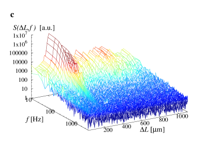
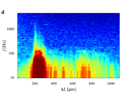
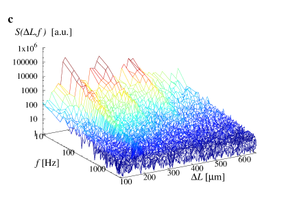
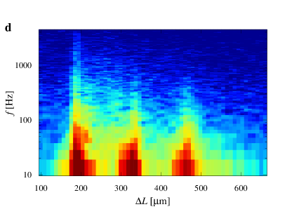
Figure 4: Dynamically enhanced OCT measurements of thermal fluctuations of the structure of a finger and those of a sweetfish eye: a,b, Thermal fluctuation spectra for the cross-sections of a finger, and the contour plot. c,d, Thermal fluctuation spectra of the cross-sections of a sweetfish eye, and the contour plot.

In Fig. 4a,b, dynamical enhanced OCT images of a finger (palm forward direction), and in Fig. 4c,d those of a sweetfish eye are shown. Here, the media are quite inhomogeneous, and the thermal spectra of reflective surfaces can be seen continually. The observed spectra for the cross-sections do not seem to correspond to the spectra of simple fluids like oil, water or elastic materials, and more investigation is necessary to determine their properties. The dependence of the sweetfish eye surface fluctuation spectrum on the moisture level of the surface has been observed previouslyMA1 , and the dependence of the depth resolved spectra on moisture levels would be of interest.

V Summary and discussions

In this work, we have developed a system dynamically enhancing OCT, and demonstrated that thermal height fluctuations, hence the physical properties of each cross-section in OCT, can be obtained this way. Required extra instrumentation over OCT is minimal, while essentially doubling the measurement apparatus if noise reduction is incorporated. We restricted our attention to thermal fluctuations in this work, which are spontaneous, and are at the atomic scale. However, the system can be applied to motions, and also to fluctuations that have been excited externally. Their power spectra can have larger magnitudes, and consequently be easier to measure.

References

- (1) N. Tanno, T. Ichikawa, A. Saeki, “Lightwave Reflection Measurement”, Japanese Patent #2010042 (1990).
- (2) D. Huang, et al, “Optical coherence tomography” Science 254, 1178-1181 (1991).
- (3) A.F. Fercher, W. Drexler, C.K. Hitzenberger, T. Lasser, “Optical coherence tomography - principles and applications”, Rep. Prog. Phys. 66, 239—303 (2003).
- (4) A.F. Fercher, C.K. Hitzenberger, G. Kamp, S.Y. Elzaiat, “Measurement of intraocular distances by backscattering spectral interferometry”, Opt. Comm. 117, 43—48 (1995).
- (5) G. Hausler, M.W. Lindner, “Coherence radar” and ”spectral radar” – new tools for dermatological diagnosis”, J. Biomed. Opt. 3, 21-31 (1998).
- (6) T. Mitsui, “Dynamic range of optical reflectometry with spectral interferometry”, Jpn. J. Appl. Phys. 38, 6133—6137 (1999).
- (7) R. Leitgeb, C.K. Hitzenberger, A. Fercher, “Performance of fourier domain vs. time domain optical coherence’ tomography”, Opt. Exp. 11, 889—894 (2003).
- (8) J.F. de Boer et al, “Improved signal-to-noise ratio in spectral-domain compared with time-domain optical coherence tomography”, Opt. Lett. 28, 2067—2069 (2003).
- (9) X.J. Wang, T.E. Milner, J.S. Nelson, “Characterization of fluid-flow velocity by optical doppler tomography”, Opt. Lett. 20, 1337—1339 (1995).
- (10) S. Makita et al, “Optical coherence angiography”, Opt. Express, 14, 7821—7840 (2006).
- (11) A.Q. Zhang, Q.Q. Zhang, C.L. Chen, R.K.K Wang, “Methods and algorithms for optical coherence tomography-based angiography: a review and comparison”, J. Biomed. Opt. 20, 100901 (2015).
- (12) D. Langevin (ed), “Light scattering by liquid surfaces and complementary techniques”, Marcel Dekker, New York (1992).
- (13) P. Cicuta, L. Hopkinson, “Recent developments of surface light scattering as a tool for optical-rheology of polymer monolayers”, Colloids and Surfaces A: Physicochem. Eng. Aspects 233, 97—107 (2004).
- (14) L.M.C. Sagis, “Dynamic properties of interfaces in soft matter: Experiments and theory”, Rev. Mod. Phys. 83, 1367—1403 (2011).
- (15) E.A. Swanson, et al, “High-speed optical coherence domain reflectometry”, Opt. Lett. 17, 151—153 (1992).
- (16) T. Mitsui, K. Aoki, “ Direct optical observations of surface thermal motions at sub-shot noise levels”, Phys. Rev. E80, 020602(R) (2009).
- (17) Shin-Etsu Chemical Co., Ltd, https://www.shinetsusilicone-global.com/catalog/index.shtml.
- (18) W.M. Haynes, “CRC Handbook of Chemistry and Physics, 92nd Edition”, CRC Press (Baton Rouge, 2011).
- (19) V.G. Levich, “Physicochemical Hydrodynamics”, Prentice-Hall, Englewood Cliffs (1962).
- (20) M.-A. Bouchiat, J. Meunier, “Power spectrum of fluctuations thermanny excited on free surface of a simple liquid”, J. de Phys. 32, 561—571 (1971).
- (21) J. Jackle, “The spectrum of surface waves on viscoelastic liquids of arbitrary depth”, J. Phys. Cond. Matt. 10, 7121—7131 (1998).
- (22) T. Mitsui and K. Aoki, “Measurements of liquid surface fluctuations at sub-shot-noise levels with Michelson interferometry”, Phys. Rev. E 87, 042403 (2013).