Universal shape characteristics for the mesoscopic star-shaped polymer via dissipative particle dynamics simulations

Abstract

In this paper we study the shape characteristics of star-like polymers in various solvent quality using a mesoscopic level of modeling. The dissipative particle dynamics simulations are performed for the homogeneous and four different heterogeneous star polymers with the same molecular weight. We analyse the gyration radius and asphericity at the bad, good and $\theta$-solvent regimes. Detailed explanation based on interplay between enthalpic and entropic contributions to the free energy and analyses on of the asphericity of individual branches are provided to explain the increase of the apsphericity in $\theta$-solvent regime.

Keywords: star-like polymer, $\theta$-solvent, dissipative particle dynamics

1 Introduction

Star polymers represent the simplest case of branched polymers, consisting of $f$ linear chains connected to the central core. The central core can be an atom, or a molecule or even a macromolecule. The first synthesis of star polymers was made by Shaefgen and Flory [1] in 1948. More than ten years later Morton et al. [2] have synthesized the 3- and 4-branch polystyrene stars. Since then the methods of synthesis have been drastically improved. Currently, there are several general methods ti synthesis star polymers: using multifunctional linking agents or multifunctional initiators and via difunctional monomers [3, 4]. There are several important polymerization techniques, i.e. cationic, anionic, controlled radical, ring opening, group transfer, step-growth polycondensation and their combinations (see Ref. [5] and references therein). Substantial interest in theoretical and experimental studies of star polymers arises due to their important applications. by their practical applications importance. Star polymers may have a properties much different from those of the linear chain polymers. They have more compact size and, therefore, higher segment density compared to their linear counterparts with the same molecular weight. This feature affects substantially the properties of the star polymer containing systems [3, 4]. Their bulk viscosity in concentrated as well as in dilute solution, can be lower than for a linear polymers of similar molecular weight. Besides that star polymers can self-assemble in more types of microstructures, which can be promoted in solutions due to the presence of the functional groups in their branches, or by using a selective solvent in the case of star-block or miktoarm star copolymers, leading to the formation of micellar structures [6].

In terms of molecular topology, star polymers represent an intermediate system between linear chain polymers and colloidal particles such as polystyrene and silica spheres. This feature has been discussed in a number of papers, in which the structure [7, 8, 9, 10] and dynamics [11, 12, 13, 14, 15, 16, 17, 18, 19] of the star polymers have been studied. The properties of the stars with a small number of branches are similar to those of the linear chain polymers. In particular, their average configuration is characterized by a large aspherisity [20, 21]. The star structures with larger number of the branches have much lower aspherisity and in the limit of large $f$ they can be seen as rigid spherical particles [22]. Star polymers have substantially higher shear stability [23] and they are widely used as viscosity index modifier in the multigrade lubricating oils [24, 25]. They are also used for manufactoring the thermoplastic elastomers, which at room temperature have the properties similar to those of cross-linked elastomers (such as vulcanized rubber). However, with the temperature increase, they became soft and can flow, which is a very useful property for their processing [26]. In addition, thermoplastic elastomers, in contrast to rubber, can be reused. For producing thermoplastic elastomers the mixture of linear and miktoarm star triblock copolymers is often used [26]. Star polymer systems are used in coating materials, as binders for toners for copying machines [8], resins for electrophotographic photoreceptors [27] and in a number of pharmaceutical and medical applications [28, 8]. Star polymers and starburst dendrimers also have important applications in semiconductor devices [29], in biofunctionalized patterning of the surfaces [30], and in controlled release drug delivery [31]. Reviews of the synthesis, properties and applications of star polymers are given in Ref. [5].

Due to the substantial advances in the synthesis of star polymers, as well as their numerous applications, they have attracted considerable interest both theoretical and experimental methods [3, 4, 8, 5, 6]. Theoretical studies of the polymer stars were carried out using renormalization group [32, 33, 34, 35, 36, 37, 38, 39, 40, 41, 42, 43] (see also Ref. [44] and references therein) and the field theoretical [45, 46, 47] approaches, extrapolation of exact enumerations [48, 49, 50, 51], free energy minimization method [52, 53, 54], mean field [55, 56, 57] and scaling theories [58, 59, 60, 61, 62, 63, 64, 65, 66], as well as the density functional approach [67]. In general, the properties of polymers have been studied intensively in the past using computer simulations methods, such as molecular dynamics and Monte-Carlo methods [68, 69, 70, 71, 72]. These methods were also used to study the properties of the star polymers and a large number of corresponding studies have been published during the last decade (see Ref. [73] and references there in).

One of important properties of star polymers that affect their technological application is their shape. Conformational and shape properties of the star polymers, which include mean square radius of gyration and hydrodynamic radii, were studied experimentaly [74, 75, 76, 77, 78]. The universal shape properties of the linear chain polymers in a form of a self-avoiding walk (SAW) were also studied recently via lattice modeling [79, 80, 22, 81, 82, 83, 84, 85, 86]. It was demonstrated that certain shape properties of polymer chains, similar to the scaling exponents, are universal and depend solely on dimensionality of the space $d$. This type of the approach appears to be very efficient and allows one to achieve very good configuration statistics by means of a relatively low computational cost. However, the lattice models are not able to easily account for the effects of chain stiffness, chain composition, the quality of a solvent, etc. On the other hand, atomistic first principal simulations [87], which can include all these features, require substantial amount of the computer time. Perhaps, the most adequate computer simulation method to be used, which is able to compromise between chemical versatility and computational efficiency, is the dissipative particle dynamics (DPD) method. Applications of this method to the case of star polymers are already present [88, 89, 90, 91, 92, 93, 94]. In particular, in the paper of Nardai and Zifferer [87], dilute solutions of linear star polymers have been studied using DPD simulations. On the other hand, in our previous paper [95] we applied the DPD method to investigate the shape characteristics of a linear polymer chain in a good solvent. We have shown that such shape properties of the chain as asphericity, prolateness and some other are universal. The paper may be regarded as an extension of our work [95] on shape properties of linear polymer chains aiming at systematic analysis of the combined impact of solvent quality and polymer topology of the polymer shape properties. The aim of this study is to apply the same analysis to the case of star polymers. The outline of the paper is as follows. Sec. 2 contains detailed description of the model star polymers and the properties of interest to be studied. Sec. 3 contains the results and their interest. Conclusions are given in Sec. 4.

2 The model, simulation approach and properties of interest

As already mentioned in Sec. 1, our study is based on the mesoscopic DPD simulation technique. In this approach, the monomers, as well as the solvent beads, represent respective groups of atoms. They are soft spheres of equal size, repulsive to each other.Therefore, the DPD technique enables one to consider both the effects of a star-like topology as well as solvent quality via explicit account of mesoscopic polymer-solvent and solvent-solvent interactions

                   

4:0                                   2:0                                   0:0

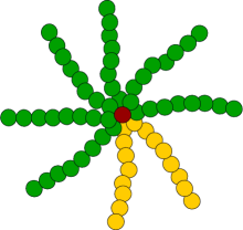
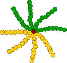
0:2                             0:4

Figure 1: Sketches of polymer stars considered in this paper. Each star consists of $f_{A}+f_{B}+f_{C}=8$ branches of equal length of $N_{f}=8$ monomers attached to the central core (red sphere). $f_{A}$ and $f_{B}$ denotes the number of solvophilic and solvophobic branches, respectively, $f_{C}$ stands for branches with variable solvophobicity. For the homogeneous star ($f_{A}=0$, $f_{B}=0$, further denoted as 0:0), all $f_{C}=8$ branches have the same solvophobicity, that varies from the good solvent to bad solvent regime. For the heterogeneous stars (4:0, 2:0, 0:2, 0:4), the blue $f_{A}$ branches do not change their solvophobicity remaining always solvophilic while the yellow $f_{B}$ branches are always solvophobic, whereas solvophobicity of the green $f_{C}$ branches varies.

We follow DPD method as formulated in Ref. [96]. The following reduced quantities are used: the length will be measured in units of the diameter of the soft bead, and the energy in units of $k_{B}T$. Here, $k_{B}$ is the Boltzmann constant and $T$ is the temperature. The monomers of each branch are connected via harmonic springs, which results in the force

$$\mathbf{F}^{B}_{ij}=-k\mathbf{x}_{ij}\,,$$ (1)

where $\mathbf{x}_{ij}=\mathbf{x}_{i}-\mathbf{x}_{j}$, $\mathbf{x}_{i}$ and $\mathbf{x}_{j}$ are the coordinates of $i$th and $j$th bead, respectively, and $k$ is the spring constant. The total force acting on the $i$th bead from the $j$th one can be denoted as

$$\mathbf{F}_{ij}=\mathbf{F}^{\mathrm{C}}_{ij}+\mathbf{F}^{\mathrm{D}}_{ij}+\mathbf{F}^{\mathrm{R}}_{ij}\,,$$ (2)

where $\mathbf{F}^{\mathrm{C}}_{ij}$ is the conservative force responsible for the repulsion between the beads, $\mathbf{F}^{\mathrm{D}}_{ij}$ is the dissipative force that defines the friction between them and the random force $\mathbf{F}^{\mathrm{R}}_{ij}$ works in pair with a dissipative force to thermostat the system. The expression for all these three contribution are given below [96]

$$\mathbf{F}^{\mathrm{C}}_{ij}=\left\{\begin{array}[]{ll}a(1-x_{ij})\displaystyle\frac{\mathbf{x}_{ij}}{x_{ij}},&x_{ij}<1,\\ 0,&x_{ij}\geq 1,\end{array}\right.$$ (3)

$$\mathbf{F}^{\mathrm{D}}_{ij}=-\gamma w^{\mathrm{D}}(x_{ij})(\mathbf{x}_{ij}\cdot\mathbf{v}_{ij})\frac{\mathbf{x}_{ij}}{x^{2}_{ij}},$$ (4)

$$\mathbf{F}^{\mathrm{R}}_{ij}=\sigma w^{\mathrm{R}}(x_{ij})\theta_{ij}\Delta t^{-1/2}\frac{\mathbf{x}_{ij}}{x_{ij}},$$ (5)

where $x_{ij}=|\mathbf{x}_{ij}|$, $\mathbf{v_{ij}}=\mathbf{v}_{i}-\mathbf{v}_{j}$, $\mathbf{v}_{i}$ is the velocity of the $i$th bead, $a$ is the amplitude for the conservative repulsive force. The dissipative force has an amplitude $\gamma$ and decays with distance according to the weight function $w^{\mathrm{D}}(x_{ij})$. The amplitude for the random force is $\sigma$ and the respective weight function is $w^{\mathrm{R}}(x_{ij})$. $\theta_{ij}$ is the Gaussian random variable. As was shown by Español and Warren [97], to satisfy the detailed balance requirement, the amplitudes and weight functions for the dissipative and random forces should be interrelated: $\sigma^{2}=2\gamma$ and $w^{\mathrm{D}}(x_{ij})=\large[w^{\mathrm{R}}(x_{ij})\large]^{2}$. Here we use quadratically decaying form for the weight functions:

$$w^{\mathrm{D}}(x_{ij})=\large[w^{\mathrm{R}}(x_{ij})\large]^{2}=\left\{\begin{array}[]{ll}(1-x_{ij})^{2},&x_{ij}<1,\\ 0,&x_{ij}\geq 1.\end{array}\right.$$ (6)

The reduced density of the system is defined as $\rho^{*}=(N+N_{s})/V=3$ , where $N_{s}$ is the number of solvent particles and $V$ is system volume. The other parameters are chosen as follows: $\gamma=6.75$, $\sigma=\sqrt{2\gamma}=3.67$

Parameter $a$ in the conservative force $\mathbf{F}^{\mathrm{C}}_{ij}$ defines maximum repulsion between two beads which occurs at their complete overlap, $x_{ij}=0$. We consider three types of branches: solvophilic (beads of type $A$), solvophobic (beads of type $B$) and with variable solvophobicity (beads of type $C$). Their respective numbers are $f_{A}$, $f_{B}$ and $f_{C}$. Each star type is denoted as ($f_{A}:f_{B}$), and $f_{C}$ is equal to $f_{C}=f-f_{A}-f_{B}$. The solvent beads are of type $S$. The values of the repulsion parameter a are chosen according to the bead types. Namely: $a_{AA}=a_{BB}=a_{CC}=a_{SS}=a_{AS}=25$ and $a_{BS}=40$. The value of $a_{CS}$ is varied within the range from 25 (solvophilic branch) up to 40 (solvophobic branch). In what follows below, we have chosen to characterize shape of star polymers in terms of their radius of gyration and asphericity. The latter can be obtained from the eigenvalues of the gyration tensor $\mathbf{Q}$ defined as [20, 21]:

$$Q_{\alpha\beta}=\frac{1}{N}\sum_{n=1}^{N}(x^{\alpha}_{n}-X^{\alpha})(x^{\beta}_{n}-X^{\beta})\hskip 10.00002pt\alpha,\beta=1,2,3,$$ (7)

where $N$ is the number of monomers of a star polymer, $x_{n}^{\alpha}$ stands for the set of the Cartesian coordinates of $n$th monomer: $\mathbf{x}_{n}=(x_{n}^{1},x_{n}^{2},x_{n}^{3})$, and $X^{\alpha}=\frac{1}{N}\sum_{n=1}^{N}x_{n}^{\alpha}$ are the coordinates of the center of mass for the star polymer. Its eigenvectors define the axes of a local frame of a star polymer and the mass distribution of the latter along each axis is given by the respective eigenvalues $\lambda_{i}$, $i=1,2,3$. The trace of $\mathbf{Q}$ is an invariant with respect to rotations and is equal to an instantaneous squared gyration radius of the star polymer

$$R_{g}^{2}=\mathrm{Tr}\,\mathbf{Q}=\sum_{i=1}^{3}\lambda_{i}=3\bar{\lambda}$$ (8)

Here, the arithmetic mean of three eigenvalues, $\bar{\lambda}$, is introduced to simplify the forthcoming expressions. The asphericity $A$ [79, 22, 81, 86] for the three-dimensional case is defined as

$$A=\frac{1}{6}\frac{\sum_{i=1}^{3}(\lambda_{i}-\bar{\lambda})^{2}}{\bar{\lambda}^{2}}.$$ (9)

By definition, an inequality holds: $0\leq A\leq 1$ [86]. The asphericity equals zero for an ideally spherical shape, when all eigenvalues are equal: $\lambda_{i}=\bar{\lambda}$. On the other extreme, an asphericity of a rod, when all eigenvalues but one vanish, $A=1$. In the course of simulations, the instantaneous value $A$ is then averaged over time trajectory of simulations, this averaged value is denoted as $\langle A\rangle$.

3 Results

As already discussed in Sec. 2, we consider four types of heterogeneous stars and a homogeneous star copolymer, see Fig. 1. The linear size of a cubic simulation box is chosen to be at least four gyration radius of a single branch in a coiled conformation. For each heterogeneous star we perform $2\cdot 10^{6}$ DPD steps, whereas for a homogeneous star the simulation length is $6\cdot 10^{6}$ DPD steps, for each considered value of $a_{CS}$. The time step is $\bigtriangleup t^{*}=0.04$. To estimate statistical errors of particular characteristic $x$, the simulation time trajectory is divided into four equal intervals. In each i$th$ interval we calculate its partial simple average value $\langle x\rangle^{[i]}$ and the histogram for its distribution $P^{[i]}(x)$.

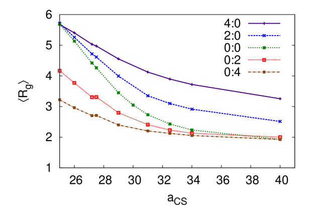
Figure 2: Mean gyration radius $\langle R_{g}\rangle$ of the ($f_{A}:f_{B}$) polymer star as a function of $a_{CS}$. Here $f_{A}$ is a number of solvophilic branches and $f_{B}$ is a number of solvophobic branches. The rest $f_{C}=f-f_{A}-f_{B}$ branches have variable solvophilicity. The $a_{CS}$ parameter discriminates between good ($a_{CS}=25$) and bad ($a_{CS}=40$) solvent quality for the $f_{C}$ branches. Green line corresponds to a homogeneous star when $f_{C}=f$, marked as ($0:0$). Here the gyration radius is expressed in the units $\sigma$ which is the diameter of one monomer.

First we analyse the value of the gyration radius $R_{g}$ for a star polymer depending on the solvent quality. The latter was tuned by the choice of $a_{CS}$, from the good solvent case ($a_{CS}=25$) to the bad one ($a_{CS}=40$), see Fig. 2. Let us consider the change undergone by $R_{g}$ for the case of the homogeneous star (0:0), when $a_{CS}$ increases from $25$ to $40$. This change drives the conformation of all the branches from a coiled state to the collapsed one. As a consequence, the $R_{g}$ decreases smoothly from $5.8$ down to $2$. For the heterogeneous stars with fixed solvophilic branches ($4:0$ and $2:0$), the $R_{g}$ value at $a_{CS}=25$ is, obviously, the same as the one for the homogeneous star. But at $a_{CS}=40$ the gyration radius for both $(4:0)$ and $(2:0)$ stars have higher magnitude due to the fact that $f_{A}$ branches are still in a coiled state, whereas the other $f_{C}$ branches are in a collapsed state. On contrary, heterogeneous stars with fixed solvophobic branches $(0:2)$ and $(0:4)$ have the same value of $R_{g}$ at $a_{CS}=40$ as the homogeneous star and a lower value at $a_{CS}=25$. This is, obviously, due to the fact that at $a_{CS}=25$ only $f_{C}$ branches are in a coil state, whereas the other $f_{B}$ branches are always in a collapsed state.

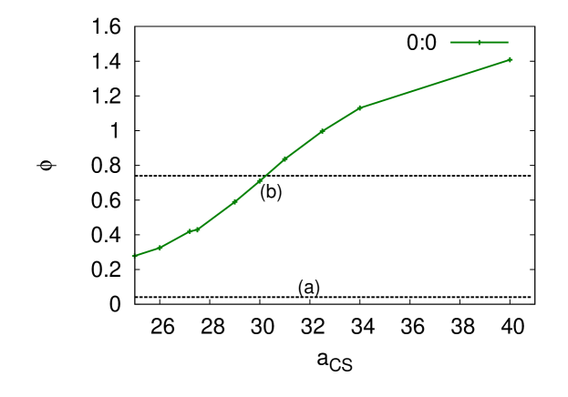
Figure 3: Solid line: packing fraction $\phi$ of the homogeneous star ($0:0$) at various $a_{CS}$, the solvophobicity of its beads. Dashed lines: packing fractions of the case when all branches are fully stretched (a) and when they are tightly packed(b)

In the DPD method all the beads are soft and can overlap, unlike for the hard spheres model. To quantify this effect, we analysed the packing fraction $\phi$ of beads depending on the solvent quality, see Fig. 3. It is given by

$$\phi=\frac{N_{b}\frac{4}{3}\pi r^{3}}{V_{glob}}$$ (10)

where $N_{b}$ is the number of beads in a star polymer, $r$ is the radius of a single bead and $V_{glob}$ is the volume occupied by star polymer. This volume can be expressed $via$ the expression $V_{glob}=\frac{4}{3}\pi R^{3}$, where $R$ is the radius of an equivalent sphere with the same volume as that of a star polymer. We estimate $R$ from its relation to the gyration radius $R_{g}$. As the first approximation, one can take the relation $R=\sqrt{\frac{5}{3}}R_{g}$ which holds for a solid spheres. We also display in Fig. 3 the packing fractions that relate to two limiting cases. These are marked as $(a)$: the case when all the branches are in a fully stretched conformation and $(b)$, when the star polymer comprises a compact object of tightly packed hard spheres. In the good solvent regime at $a_{CS}=25$, the packing fraction is $\phi\approx 0.28$ which is close to the case $(a)$. At $a_{CS}=30$, the packing fraction crosses the line $(b)$. With an increase of $a_{CS}$ the packing fraction increases, and in the bad solvent regime at $a_{CS}=40$, $\phi$ is equal to $1.4$. It is indicating severe beads overlap, and, hence highly compressed state of the star polymer.

Let us switch our attention to the asphericity of the stars. The histograms $P^{[i]}(A)$ for the distribution of asphericity in each $[i]$th interval $A$ are presented in Fig. 4 for the case of homogeneous star at $a_{CS}=27.5$. This value was estimated earlier in Ref. [87] as the one providing approximately the $\theta$-conditions for similar model of a star polymer. We observe that the data points obtained for each $P^{[i]}(A)$ follow the same curve. The shape of this curve, similarly to the case of linear polymer chain [95], can be approximated well by the Lhuillier-type distribution:

$$P_{L}(A)=B\exp\left[-\Big{(}\frac{A^{\prime}}{A}\Big{)}^{\epsilon_{1}}-\Big{(}\frac{A}{A^{\prime}}\Big{)}^{\epsilon_{2}}\right],\;\;\;A_{max}=A^{\prime}\Big{(}\frac{\epsilon_{1}}{\epsilon_{2}}\Big{)}^{\frac{1}{\epsilon_{1}+\epsilon_{2}}}.$$ (11)

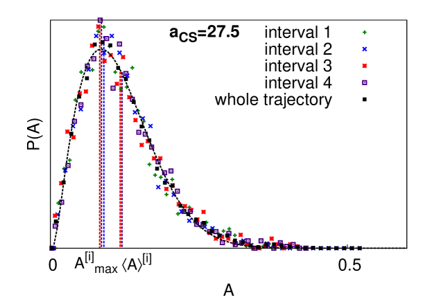
Figure 4: Distribution of the asphericity $A$ of a homogeneous star at solvent quality $a_{CS}=27.5$ for the intervals 1: $0<N_{stp}<15\cdot 10^{5}$, 2: $15\cdot 10^{5}<N_{stp}<3\cdot 10^{6}$, 3: $3\cdot 10^{6}<N_{stp}<45\cdot 10^{5}$, 4: $45\cdot 10^{5}<N_{stp}<6\cdot 10^{6}$, as well as for the whole simulation $0<N_{stp}<6\cdot 10^{6}$. Black curve is fitting according to Eq. 11

Here $A_{max}$ is the position of the maximum for the $P_{L}(A)$ and $B,A^{\prime},\epsilon_{1}$ and $\epsilon_{2}$ are fitting parameters. We perform the separate fit for each $P^{[i]}(A)$ to the form Eq. (11) resulting in a set of parameters $B^{[i]},A^{\prime[i]},\epsilon_{1}^{[i]},\epsilon_{2}^{[i]}$ and $A_{max}^{[i]}$. The sets provide both the respective averages for each of these parameters, as well as their standard deviations evaluated within the set. The same procedure is used for all values of $a_{CS}=25-40$. The results for the simple average of the asphericity $\langle A\rangle$, and the average position of the maximum $A_{max}$, alongside with their respective errors are shown in Fig. 5. Similarly to the data shown in Fig. 4, the magnitude of $\langle A\rangle$ is higher than that for $A_{max}$. However, the changes undergone by both characteristics with the variation of $a_{CS}$ are very similar. Namely, both increase within the interval $25<a_{CS}<29$, peak at approximately $a_{CS}=29$ and then both decay. For both characteristics we observe a maximum at the interval $27<a_{CS}<29$. This interval contains the value $a_{CS}=27.5$ estimated as a $\theta$-point by Nardai and Zifferer [87], for the same simulations model. Below we attempt to clarify the reason for this maxima.

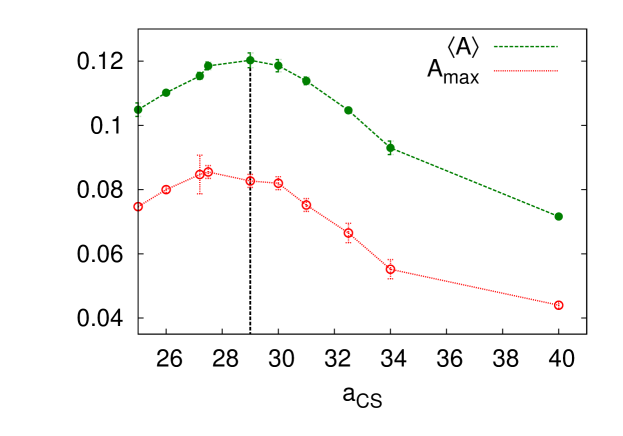
Figure 5: Plot of the asphericity of a homogeneous star as a function of the solvophobicity of its beads $a_{CS}$ . Here $\langle A\rangle$ and $A_{max}$ are the mean and maximal values of $A$ is found from the distribution (11).

To clarify this peculiarity of the asphericity at the $\theta$-condition, we will consider the asphericity of the heterogeneous stars, depicted in Fig. 6. The cases $(2:0)$ and $(4:0)$ at $a_{CS}=25$ are characterized by all the branches being in a coiled state, similarly to the case $(0:0)$ at the same $a_{CS}$. Hence, the same value of $\langle A\rangle=0.105$ is observed in all cases mentioned above. With the $a_{CS}$ value approaching 40, the $(0:2)$ and $(0:4)$ stars at $a_{CS}=40$ have all their branches collapsed. Again, this mimics the case of $(0:0)$ star at $a_{CS}=40$. Therefore, not surprisingly, the $\langle A\rangle$ values for those stars are close to the respective value of $0.075$ for the homogeneous star (cf. Figs. 5 and 6). However, cases $(0:2)$ and $(0:4)$ at $a_{CS}=25$ both have a higher asphericity value of $\langle A\rangle=0.12$, the same as for the case $(2:0)$ and $(4:0)$ at $a_{CS}=40$. This higher value of $\langle A\rangle$ is observed due to the fact that in all these cases some branches are in a coiled state and the other branches are collapsed. It is instructive to note that the same value $\langle A\rangle=0.12$ is also observed for the homogeneous star ($0:0$) in the interval $27<a_{CS}<29$. This leads us to the idea that the maxima of $\langle A\rangle$ for the ($0:0$) star, observed in this interval might be related to the coexistence of both coiled and collapsed configurations of the branches, in a $\theta$-solvent regime.

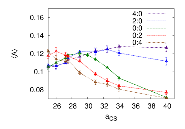
Figure 6: Asphericity $A$ of the ($f_{A}:f_{B}$) polymer star as a function of $a_{CS}$, the solvophobicity of the $C$ beads Here $f_{A}$ is a number of solvophilic branches and $f_{B}$ is a number of solvophopic branches . Factor $a_{CS}$ discriminates between good ($a_{CS}=25$) and bad ($a_{CS}=40$) solvent quality. Green line corresponds to a homogeneous star with all branches of changing solubility ($0:0$).

There different conditions for the individual branches of homogeneous star polymer, namely the cases of good, bad and the $\theta$-solvent, are illustrated in Fig. 7. These cases are considered in terms of the interplay between the enthalpic, $U$, and the entropic $S$, contributions to the free energy $F=U-TS$, with $T$ being the temperature. The case of a good solvent ($a_{CS}=25$) is displayed in Fig. $\ref{fig9}(a)$. Here all the branches are in a coiled state and are surrounded by a solvation shell. In this case, there is an effective repulsion between branches, leading to the non-zero enthalpy contribution $U$. For the case of a bad solvent, Fig. $\ref{fig9}(c)$, the branches strongly repel each other strongly by a solvent, leading to their collapse, this is interpreted as the effective solvent-mediated attraction between branches. In this case, the contribution of $U$ to the free energy is also non-zero. The intermediate case, where polymer is in the $\theta$-solvent condition, is characterized by vanishing of the enthalpy contribution $U$ and the free energy is driven now only by the entropy. As a consequence, all branches turn into the ideal chains, their conformations are uncorrelated and each one can be interpreted as a random walk. This may lead to the coexistence of both coiled and collapsed configurations of individual chains, as illustrated schematically in Fig. $\ref{fig9}(b)$.

                   

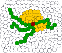
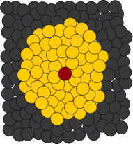
$(a)$                                $(b)$                                      $(c)$

Figure 7: Schematic illustration for the coformation of individual branches of homogeneous star polymer $(0:0)$ in various regimes. $(a)$ good solvent, $(b)$ $\theta$-condition and $(c)$ bad solvent.

To confirm this interpretation of the behavior of the star polymer in the $\theta$-solvent we conducted the analyses of the configurations of individual branches. The histogram for the distribution $p(\alpha)$ for the asphericity $\alpha$ of individual branches is illustrated in Fig. 8 for the homogeneous star at $a_{CS}=25,27.5,30$ and $40$. The general shape of this distribution changes essentially when $a_{AC}$ varies from $25$ to $40$. In general, it shows the presence of two maxima. Therefore, we fitted the data by a double Gaussian distribution:

$$p(a)=A^{\prime}\exp\left[-\Big{(}\frac{{x-\alpha^{\prime}}}{\sigma^{\prime}}\Big{)}^{2}\right]+A^{\prime\prime}\exp\left[-\Big{(}\frac{{x-\alpha^{\prime\prime}}}{\sigma^{\prime\prime}}\Big{)}^{2}\right],$$ (12)

where $A^{\prime}$ and $A^{\prime\prime}$ are respective weights, $\alpha^{\prime}$ and $\alpha^{\prime\prime}$ - respective position of two maxima, $\sigma_{1}$ and $\sigma_{2}$ are the respective dispersions. The results of the fits for $A^{\prime},A^{\prime\prime},\alpha^{\prime}$ and $\alpha^{\prime\prime}$ are collected in Tab. 1.

$a_{CS}$	25	27.5	30	40
$\alpha^{\prime}$	0.257	0.225	0.212	0.205
$A^{\prime}$	1.056	1.266	1.289	1.811
$\alpha^{\prime\prime}$	0.555	0.512	0.435	0.402
$A^{\prime\prime}$	1.683	1.617	1.587	1.514

Table 1: $\alpha^{\prime}$ and $\alpha^{\prime\prime}$ are the positions of the maxima, $A^{\prime}$ and $A^{\prime\prime}$ are the respective weights of the Gaussian distributions and $\sigma^{\prime}$ and $\sigma^{\prime\prime}$ are the respective dispersion.

Based on these results and the shape of the $p(a)$ distribution, we can deduct the following conclusion. In all cases $a_{CS}=25-40$ we see the coexistence of typical conformations, one with lower asphericity, $\alpha^{\prime}\approx 0.2-0.26$, and another one with a higher asphericity, $\alpha^{\prime\prime}\approx 0.4-0.56$. For the case of $a_{CS}=40$ low asphercity conformations prevail, as far as $A^{\prime}>A^{\prime\prime}$. Here all branches are in the collapsed state and the distribution has one maximum near $\alpha^{\prime}=0.25$. On the contrary, at $a_{CS}=25$ we have $A^{\prime}<A^{\prime\prime}$, hence the conformations with higher aspericity prevail. This is due to the branches being predominately found in a coiled state. At $a_{CS}=27.5-30$ the distribution clearly has two maxima. This evidences the coexistence of rather collapsed conformations with those that are more close to a coiled state. Hence, at the $\theta$ condition of a star polymer, there is much higher degree of the solvent regime for conformational freedom of its branches, and as a consequence, by a coexistence of more coiled conformation with the ones closer to a collapsed state. This explains the maximum for the average asphericity $\langle A\rangle$ as observed in Fig. 5.

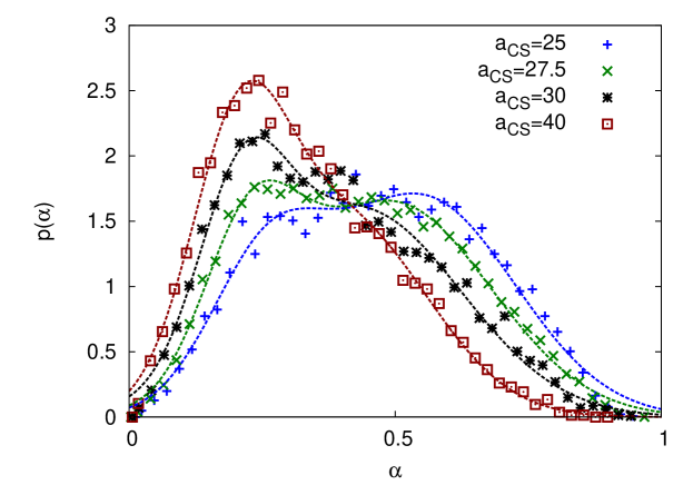
Figure 8: Distribution of asphericity $p(\alpha)$ of individual branches of a homogeneous star at various solvophobicity of its branches $a_{CS}$.

4 Conclusions

We have analysed the shape characteristics of the coarse-grained heterogeneous and homogeneous star-like polymers at various solvent quality using the DPD simulations. The heterogeneous star is characterized by different solvophobicity of its individual branches. The solvent quality was tuned by varying the parameter $a_{CS}$ for the repulsive conservative force of the branches with variable solvophobicity. For homogeneous and four types of heterogeneous star polymers, the gyration radius decreases with the increase of the repulsion parameter $a_{CS}$ indicating a collapsed state for the part or all their branches. The packing fraction $\phi$ at $a_{CS}=30$ is close to the packing fraction of the hexagonally packed hard spheres. We found an interesting effect that, upon the change of solvent properties, the asphericity of a homogeneous star reaches its maximum value when the solvent is near $\theta$-point. The effect is explained by the interplay between the enthalpic and entropic contributions to the free energy. In particular, at the $\theta$-point condition, the enthalpic contribution vanishes and the branch conformation are driven exclusively by the entropy. This provides means for the wider spectra of possible conformations from collapsed to the coiled ones. We check this explanation by the analyses of the asphericity of the individual branches. Their distribution near $\theta$-condition has two maxima, which is well fitted by double Gaussian distribution. This confirms the coexistence of two types of conformation, namely, more coiled and more collapsed ones. An extension of this analyses to the case of aggregation of star-like polymers into micelles which has applications for the drug delivery systems will be the subject of the forthcoming paper.

5 Acknowledgements

This work was supported in part by FP7 EU IRSES project No. 612707 ”Dynamics of and in Complex Systems” and No. 612669 ”Structure and Evolution of Complex Systems with Applications in Physics and Life Science”. J.I. acknowledges Alexander Blumen for stimulating discussions towards the interpretation of the result.

References

- [1] Schaefgen J R and Flory P J 1948 Journal of the American Chemical Society 70 2709–2718.
- [2] Morton M, Helminiak T E, Gadkary S D and Bueche F 1962 Journal of Polymer Science 57 471–482.
- [3] Mishra M and Kobayashi S 1999 Star and hyperbranched polymers vol 53 (CRC Press).
- [4] Hadjichristidis N, Pitsikalis M, Pispas S and Iatrou H 2001 Chemical Reviews 101 3747–3792.
- [5] Hadjichristidis N, Pitsikalis M, Iatrou H, Driva P, Sakellariou G and Chatzichristidi M 2012 29–111.
- [6] Khanna K, Varshney S and Kakkar A 2010 Polymer Chemistry 1 1171.
- [7] Gast A P 1996 Langmuir 12 4060–4067
- [8] Grest G, Fetters L, Huang J and Richter D 1996 Polymeric Systems; Prigogine, I.; Rice, SA, Eds.; Wiley: New York 94 67–163
- [9] Likos C N, Löwen H, Watzlawek M, Abbas B, Jucknischke O, Allgaier J and Richter D 1998 Physical Review Letters 80 4450–4453
- [10] Witten T A and Pincus P A 1986 Macromolecules 19 2509–2513
- [11] Sikorski A 1993 Polymer 34 1271–1281
- [12] Factor B J, Russell T P, Smith B A, Fetters L J, Bauer B J and Han C C 1990Macromolecules 23 4452–4455
- [13] Vlassopoulos D, Pakula T, Fytas G, Pitsikalis M and Hadjichristidis N 1999 The Journal of Chemical Physics 111 1760–1764
- [14] Grest G S, Kremer K, Milner S T and Witten T A 1989 Macromolecules 22 1904–1910
- [15] Su S J, Denny M S and Kovac J 1991 Macromolecules 24 917–923
- [16] Su S J and Kovac J 1992 The Journal of Physical Chemistry96
- [17] Stratinf P and Wiegel F 1994 International Journal of Modern Physics B
- [18] Sikorski A and Romiszowski P 1999 Macromolecular theory and simulations 8 103–109
- [19] Ganazzoli F, Allegra G, Colombo E and Vitis M D 1995 Macromolecules
- [20] Šolc K 1971 The Journal of Chemical Physics 54 2756
- [21] Šolc K and Stockmayer W H 1971 The Journal of Chemical Physics 55 335
- [22] Zifferer G 1999 The Journal of Chemical Physics 110 4668–4677
- [23] Xue L, Agarwal U S and Lemstra P J 2005 Macromolecules 38
- [24] Lohse D J, Milner S T, Fetters L J, Xenidou M, Hadjichristidis N, Mendelson R A, García-Franco C A and Lyon M K 2002 Macromolecules 35 3066–3075
- [25] Schober B J, Vickerman R J, Leeb O D, Dimitrakisa W J and Gajanayakec A 2008 Controlled architecture viscosity modifiers for driveline fluids: Enhanced fuel efficiency and wear protection Proceedings of the 14th Annual Fuels Lubes Asia Conference
- [26] Knoll K and Nießner N 1998 Macromolecular Symposia 132
- [27] Maness K M, Masui H, Wightman R M and Murray R W 1997 Journal of the American Chemical Society 119 3987–3993
- [28] Likos and Harreis 2002 Condensed Matter Physics 5 173
- [29] Hecht S, Ihre H and Fréchet J M J 1999 Journal of the American Chemical Society 121 9239–9240
- [30] Heyes C D, Groll J, Möller M and Nienhaus G U 2007 Mol. BioSyst 3 419–430
- [31] James H P, John R, Alex A and Anoop K 2014 Acta Pharmaceutica Sinica B 4 120–127
- [32] Douglas J F, Roovers J and Freed K F 1990 Macromolecules 23 4168–4180
- [33] Shiwa Y, Oono Y and Baldwin P R 1990 Modern Physics Letters B 04 1421–1428
- [34] Merkle G, Burchard W, Lutz P, Freed K F and Gao J 1993 Macromolecules 26 2736–2742
- [35] Zhu S 1998 Macromolecules 31 7519–7527
- [36] Vlahos C H, Horta A and Freire J J 1992 Macromolecules 25
- [37] Duplantier B 1986 Physical Review Letters 57 941–944
- [38] Ohno K and Binder K 1991 The Journal of Chemical Physics 95
- [39] Ohno K and Binder K 1988 Journal de Physique 49 1329–1351
- [40] Miyake A and Freed K F 1983 Macromolecules 16 1228–1241
- [41] Miyake A and Freed K F 1984 Macromolecules 17 678–683
- [42] Vlahos C H and Kosmas M K 1987 Journal of Physics A: Mathematical and General 20 1471–1483
- [43] von Ferber C and Holovatch Y 1997 Physical Review E 56 6370–6386
- [44] von Ferber C and Holovatch Y 1999 Physical Review E 59 6914–6923
- [45] Chujo Y, Naka A, Krämer M, Sada K and Saegusa T 1995 Journal of Macromolecular Science, Part A 32 1213–1223
- [46] Okamoto S, Hasegawa H, Hashimoto T, Fujimoto T, Zhang H, Kazama T, Takano A and Isono Y 1997 Polymer 38 5275–5281
- [47] Knoll K and Nießner N 1998 Styrolux and styroflex from transparent high impact polystyrene to new thermoplastic elastomers: Syntheses, applications and blends with other styrene based polymers Macromolecular Symposia vol 132 (Wiley Online Library) pp 231–243
- [48] Lipson J E G, Whittington S G, Wilkinson M K, Martin J L and Gaunt D S 1985 Journal of Physics A: Mathematical and General 18 L469–L473
- [49] Wilkinson M K, Gaunt D S, Lipson J E G and Whittington S G 1986 Journal of Physics A: Mathematical and General 19 789–796
- [50] Barrett A J and Tremain D L 1987 Macromolecules 20 1687–1692
- [51] Colby S A, Gaunt D S, Torrie G M and Whittington S G 1987 Journal of Physics A: Mathematical and General 20 L515–L520
- [52] Ganazzoli F and Allegra G 1990 Macromolecules 23 262–267
- [53] Ganazzoli F, Fontelos M A and Allegra G 1991 Polymer 32 170–180
- [54] Ganazzoli F 1992 Macromolecules 25 7357–7364
- [55] Boothroyd A T and Ball R C 1990 Macromolecules 23 1729–1734
- [56] Boothroyd A T and Fetters L J 1991 Macromolecules 24 5215–5217
- [57] Irvine D J, Mayes A M and Griffith-Cima L 1996 Macromolecules 29
- [58] Ohno K and Binder K 1991 The Journal of Chemical Physics 95
- [59] Ohno K and Binder K 1991 The Journal of Chemical Physics 95
- [60] Halperin A and Joanny J F 1991 Journal de Physique II 1 623–636
- [61] Raphael E, Pincus P and Fredrickson G H 1993 Macromolecules 26 1996–2006
- [62] Daoud M and Cotton J 1982 Journal de Physique 43 531–538
- [63] Birshtein T and Zhulina E 1984 Polymer 25 1453–1461
- [64] Duplantier B 1986 Physical Review Letters 57 941–944
- [65] Duplantier B and Saleur H 1986 Physical Review Letters 57 3179–3182
- [66] Duplantier B and Saleur H 1987 Physical Review Letters 59 539–542
- [67] Groh B and Schmidt M 2001 The Journal of Chemical Physics 114 5450–5456
- [68] Rey A, Freire J J, Bishop M and Clarke J H R 1992 Macromolecules 25 1311–1315
- [69] Binder K 1995 Monte Carlo and molecular dynamics simulations in polymer science (Oxford University Press)
- [70] 2002 Preface to the second edition Understanding Molecular Simulation (Elsevier) pp xiii–xiv
- [71] Kotelyanskii M and Theodorou D N 2004 Simulation methods for polymers (CRC Press)
- [72] Galiatsatos V 2005 Molecular simulation methods for predicting polymer properties (Wiley-Interscience)
- [73] von Ferber and YuHolovatch 2002 Condensed Matter Physics 5 3
- [74] Allgaier J, Martin K, Räder H J and Müllen K 1999 Macromolecules 32 3190–3194
- [75] Feng X S and Pan C Y 2002 Macromolecules 35 2084–2089
- [76] Roovers J E L and Bywater S 1972 Macromolecules 5 384–388
- [77] Roovers J E L and Bywater S 1974 Macromolecules 7 443–449
- [78] Zhou L L, Hadjichristidis N, Toporowski P M and Roovers J 1992 Rubber Chemistry and Technology 65 303–314
- [79] Aronovitz J and Nelson D 1986 J. Phys. France 47 1445–1456
- [80] Cannon J W, Aronovitz J A and Goldbart P 1991 J. Phys. I France 1
- [81] Zifferer G 1999 Macromolecular Theory and Simulations 8 433–462
- [82] Jagodzinski O, Eisenriegler E and Kremer K 1992 J. Phys. I France 2 2243–2279
- [83] Bishop M and Saltiel C J 1988 The Journal of Chemical Physics 88 6594
- [84] Benhamou M and Mahoux G 1985 Journal de Physique Lettres 46 689–693
- [85] Diehl H W and Eisenriegler E 1989 J. Phys. A: Math. Gen. 22 L87–L91
- [86] Blavatska V, von Ferber C and Holovatch Y 2011 Condensed Matter Physics 14 33701
- [87] Nardai M M and Zifferer G 2009 The Journal of Chemical Physics 131 124903
- [88] Qian H J, Chen L J, Lu Z Y, Li Z S and Sun C C 2006 The Journal of Chemical Physics 124 014903
- [89] van Vliet R E, Hoefsloot H C and Iedema P D 2003 Polymer 44 1757–1763
- [90] Ilnytskyi J M and Holovatch Y 2007 Condensed Matter Physics 10 539
- [91] Xia J and Zhong C 2006 Macromolecular Rapid Communications 27 1110–1114
- [92] Chou S H, Tsao H K and Sheng Y J 2006 The Journal of Chemical Physics 125 194903
- [93] Sheng Y J, Nung C H and Tsao H K 2006 The Journal of Physical Chemistry B 110 21643–21650
- [94] Español P and Warren P B 2017 The Journal of Chemical Physics 146 150901
- [95] Kalyuzhnyi O, Ilnytskyi J M, Holovatch Y and von Ferber C 2016 Journal of Physics: Condensed Matter 28 505101
- [96] Groot R D and Warren P B 1997 The Journal of Chemical Physics 107 4423
- [97] Español P and Warren P 1995 Europhysics Letters (EPL) 30 191–196