Search For Gravitational Redshifted Absorption Lines In LMXB Serpens X-1

Abstract

The equation of state for ultra-dense matter can be tested from observations of the ratio of mass to radius of neutron stars. This could be measured precisely from the redshift of a narrow line produced on the surface. X-rays bursts have been intensively searched for such features, but so far without detection. Here instead we search for redshifted lines in the persistent emission, where the accretion flow dominates over the surface emission. We discuss the requirements for narrow lines to be produced, and show that narrow absorption lines from highly ionized iron can potentially be observable in accreting low mass X-ray binaries (low B field) which have either low spin or low inclination so that Doppler broadening is small. This selects Serpens X-1 as the only potential candidate persistent LMXB due to its low inclination. Including surface models in the broad band accretion flow model predicts that the absorption line from He-like iron at 6.7 keV should be redshifted to $\sim 5.1~{}\mathchar 45\relax~{}5.7$ keV (10 - 15 km for $1.4\mathrm{M_{\odot}}$) and have an equivalent width of $0.8~{}\mathchar 45\relax~{}8$ eV for surface temperatures of $7~{}\mathchar 45\relax~{}10\times 10^{6}$ K. We use the high resolution Chandra grating data to give a firm upper limit of $2~{}\mathchar 45\relax~{}3$ eV for an absorption line at $\sim 5$ keV. We discuss possible reasons for this lack of detection (the surface temperature and the geometry of the boundary layer etc.). Future instruments with better sensitivity are required in order to explore the existence of such features.

1 Introduction

Neutron star masses and radii are determined by the equation of state (EoS) of dense matter, described by quantum chromodynamics (QCD) at the quark-gluon interaction level. However, this is not a theory which is well understood. Only small portions of the two dimensional phase space (temperature and chemical potential or equivalently pressure) are satisfactorily described by theory and accessible to experiment. Neutron star cores have mean densities which are much higher than can be produced in current laboratory conditions, 2 - 8 times larger than the nuclear saturation density. They are also relatively cool and in equilibrium with both strong and weak force (unlike heavy ion collider experiments) and are neutron rich (unlike normal nuclei which are approximately symmetric in neutrons and protons). Thus measuring the macroscopic properties of neutron stars gives insight into the fundamental QCD interactions in a new regime (e.g. Lattimer 2012).

The most stringent constraints so far come from the firm detection of neutron stars with masses of $\sim 2M_{\odot}$ (Demorest et al., 2010; Antoniadis et al., 2013), directly ruling out any EoS which has a maximum mass below this value. This was first thought to exclude a significant contribution of hyperons (Demorest et al., 2010), which is puzzling as they are energetically favorable at high densities. However, more recent calculations of the effect of hyperons show that these were not necessarily inconsistent with the data (e.g. Whittenbury et al. 2014).

Ideally, the full EoS can be traced out from measuring both mass and radius for a sample of neutron stars of different masses. Some of the best current constraints for this come from thermal emission from the surface of quiescent low mass X-ray binaries (LMXB), the cooling tails of thermonuclear bursts and pulse profile modelling of accreting millisecond pulsars (e.g the review by Özel & Freire 2016). However, there are multiple caveats for each technique (see e.g. Miller & Lamb 2016), and even the best determinations have uncertainties of the order of 10 - 20%.

These uncertainties could be reduced by an order of magnitude through an unambiguous measure of $M/R$ from the surface redshift of a narrow atomic line. The line is redshifted by the strong gravity of the neutron star and the redshift parameter $z$ is connected with the ratio of mass to radius by general relativity:

$$1+z=\left(1-\frac{2GM}{c^{2}R}\right)^{-0.5}$$

Emission from the neutron star surface dominates during X-ray bursts, so these have been extensively studied. Cottam et al. (2002) reported the detection of Fe XXVI/XXV and O VIII absorption lines with $z=0.35$ from the spectra of X-ray bursts from EXO 0748-676, but these features were not reproduced in more sensitive data (Cottam et al., 2008). Subsequent determination of a high spin for this object further showed that these narrow features cannot be produced from the surface (Galloway et al., 2010). No other narrow line features have been convincingly detected to date.

We review the requirements for such absorption line features to be produced, and show that the only feasible persistent source where these might be detected is the LMXB Serpens X-1 (Section 2). We describe the expected features from models of the surface (Section 3), and use these models combined with the Suzaku broadband data to predict the equivalent width of the most prominent absorption line, Fe XXV (Section 4). Section 5 shows that these predictions are already challenged by upper limits on this feature from Chandra grating data for a high temperature surface. We discuss physical implications of our results on the thermal conductivity of neutron stars and other physical parameters, and conclude by summarizing our results.

2 Requirements for observable narrow absorption lines from the neutron star surface

We follow the discussion in the Astro-H white paper on Low-mass X-ray Binaries (Done et al., 2014). To see narrow absorption lines from the NS surface requires that there are heavy elements in the photosphere, that these are not completely ionized, that the photosphere is not buried beneath an optically thick accretion flow, and that the resulting atomic features are not substantially broadened.

Heavy elements are deposited onto the NS surface by the accretion flow. They are stopped by collisional processes, which are more efficient for higher mass/charge ions. Hence iron and other heavy elements are halted higher up in the photosphere than lower atomic number elements. They can then be destroyed by spallation bombardment (by the still energetic helium and hydrogen ions, transforming the iron nuclei to lower Z elements) or sink under gravity. The deposition and destruction rate both depend linearly on $\dot{M}$ so the steady state Fe column is around the solar abundance, independent of $\dot{M}$ for $L_{\mathrm{x}}>6\times 10^{32}$ ergs/s (Bildsten et al., 2003; Chang et al., 2005). Thus there can be iron and other heavy elements in the photosphere of an accreting NS, but not in an isolated or very quiescent neutron star.

Accreting neutron stars can have either low or high mass companion stars. The neutron stars in high mass X-ray binaries are young, and the neutron stars typically have very high magnetic fields. These broaden any potential atomic features via Zeeman splitting, with $\Delta E\sim 12~{}B/(10^{9}~{}\mathrm{G})$ eV (Loeb, 2003). By contrast, the LMXB typically have low fields with $B\leq 10^{9}~{}\mathrm{G}$, so narrow atomic features can possibly form in these systems.

The surface of a neutron star in an LMXB can only be seen if it is not hidden beneath the accretion flow. This depends on the geometry of the accreting material as well as its optical depth. In the truncated disc/hot accretion flow models, the accretion geometry changes dramatically at the spectral transition between the island and banana branches (see e.g. Done et al. 2007; Kajava et al. 2014). At low accretion rates, the accretion flow is hot and quasi-spherical interior to some truncation radius at which the thin disc evaporates (island state). There is additional luminosity from the boundary layer where the flow settles onto the surface, but the flow and boundary layer merge together, forming a single hot ($\sim 30~{}\mathchar 45\relax~{}50$ keV), optically thin(ish) ($\tau\sim 1.5~{}\mathchar 45\relax~{}2$) structure (Medvedev & Narayan, 2001). A fraction $e^{-\tau}$ of the surface emission should escape without scattering, so $\sim 10~{}\mathchar 45\relax~{}20$% of the intrinsic NS photosphere should be seen directly (see Figure 1 a and b). The temperature of this surface emission can also be seen imprinted onto the low energy rollover of the Compton spectrum and is only $\sim 0.5~{}\mathchar 45\relax~{}0.6$ keV (e.g. Sakurai et al. 2014). Figure 2 shows the ion fraction of Fe in the neutron star atmosphere assuming local thermodynamic equilibrium. At $0.5~{}\mathchar 45\relax~{}0.6$ keV, there should be a considerable fraction of iron which is not completely ionized, so atomic features could be seen (Rauch et al., 2008), though X-ray irradiation from the optically thin boundary layer could give a more complex photosphere temperature structure.

At higher mass accretion rates ($L\geq 0.1~{}\mathchar 45\relax~{}0.5~{}L_{\mathrm{Edd}}$), the thin disc extends down to the NS surface, forming a boundary layer where it impacts around the NS equator. The boundary layer is now optically thick ($\tau\sim 5~{}\mathchar 45\relax~{}10$) so hides the surface beneath it. The boundary layer itself is at the local Eddington temperature of $\sim 2.5$ keV (Revnivtsev et al., 2013). This is high enough that iron should be almost completely ionized (Figure 2 and Rauch et al. 2008), so no atomic features are expected from the luminous accretion flow. However, the vertical extent of the boundary layer depends on the accretion rate, and it only forms an equatorial belt for $L\lesssim 0.3L_{\mathrm{Edd}}$ (Suleimanov & Poutanen 2006, Figure 1 c). The pole is uncovered, so this part of the neutron star surface can be seen directly. It is heated mainly by thermal conduction from the equatorial accretion belt, so its temperature is probably cool enough for H- and He-like iron to exist.

At still higher mass accretion rates, the spreading layer extends up to the pole and the surface is completely covered by the optically thick, completely ionized accretion flow (upper banana branch and Z sources: Figure 1 d). Hence the largest fraction of surface emission should be seen from a pole-on view of a lower banana branch source, where the optically thick accretion flow is confined to an equatorial belt, or in an island state, where the accretion flow covers most of the surface but is optically thin (e.g. Sakurai et al. 2014).

The final requirement is that the atomic features are not broadened by rotation, where $\Delta E\sim 1600~{}\nu_{\mathrm{spin}}/(600~{}\mathrm{Hz})\sin i$ eV (Özel, 2013). This is a stringent constraint as typical LMXBs have $\nu_{\mathrm{spin}}=185~{}\mathchar 45\relax~{}650$ Hz (Altamirano et al., 2012; Patruno & Watts, 2012).

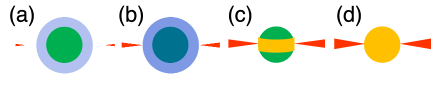
Figure 1: The geometry of the accretion flow onto the NS surface depending on the accretion rate. $L/L_{\mathrm{Edd}}$ is $\sim 10^{-4}~{}(a),\sim 10^{-2}~{}(b),\sim 0.1~{}(c),\sim 1~{}(d)$ from left to right (Done et al., 2014).

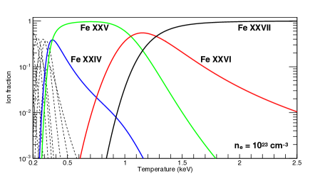
Figure 2: Ion fraction of Fe in the neutron star atmosphere. The electron density is fixed to $10^{23}~{}\mathrm{cm^{-3}}$ which is the typical value in the NS atmosphere (Özel, 2013). It is calculated using the Saha equation. We include the effect of pressure ionization by lowering the ionization potential due to Debye shielding.

There is one system, Serpens X-1, where optical spectroscopy of the 2 hour binary orbit indicates a low inclination, $i\leq 10^{\circ}$ (Cornelisse et al., 2013). A low inclination is also consistent with the non-detection of dips in the X-ray lightcurves, and the lack of any burst oscillations in the X-ray burst lightcurves (Galloway et al., 2008). This persistent system is always in the soft state (mid banana branch, $L/L_{\mathrm{Edd}}\sim 0.5$ (Chiang et al., 2016b), so the boundary layer should not extend over the pole. Additionally, this is a very bright source $\sim$ 300 mCrab. Thus Serpens X-1 is the only currently known persistent source where it may be possible to detect gravitationally redshifted lines from the surface during normal (non-burst) accretion.

3 Neutron star surface blackbody model

The emission from the hot neutron star surface should contain atomic features, which depend on the temperature, gravity and chemical composition of the photosphere. Rauch et al. (2008) show calculations for a neutron star of a mass of 1.4 M_⊙ and a radius of 10 km (i.e. $\log g=14.39$, redshift parameter $z=0.306$) and the solar abundance over the temperature range $1~{}\mathchar 45\relax~{}20\times 10^{6}$ K ($\sim$ 0.1 - 2 keV). The focus of their work was on the claimed detection of iron $n=3~{}\mathchar 45\relax~{}2$ absorption lines in EXO 0748-676 (Cottam et al., 2002), but they also show the Fe $n=2~{}\mathchar 45\relax~{}1$ absorption lines which are in a simpler part of the spectrum where there is less ambiguity in interpretation. These show that these H- and He-like K shell absorption lines are strongest around surface temperatures of 1 keV as iron is mostly ionized for temperatures above 2 keV (Figure 2). When the temperature is below 0.3 keV, the luminosity of the surface blackbody is (0.3/1)⁴ i.e. 100 times weaker so that it is difficult to observe the lines.

The neutron star surface temperature can be seen in neutron stars at low mass accretion rates (island state) as it is imprinted on the Comptonized boundary layer emission as the seed photon temperature, and distinctly hotter than the disc photons. Sakurai et al. (2014) show that this is $\sim 0.5$ keV for Aql X-1 in the brighter island states, and similar seed photon temperatures ($0.5~{}\mathchar 45\relax~{}0.7$ keV) are seen in other neutron stars in similar states (Gierliński & Done, 2002; Di Salvo et al., 2015). Higher temperatures of $1$ - $1.6$ keV are seen (again from seed photons) in the higher mass accretion rate (banana branch) states (Oosterbroek et al., 2001; Gierliński & Done, 2002; Sakurai et al., 2014; Di Salvo et al., 2015), though these are for the heated surface underneath the boundary layer rather than measuring the temperature at the uncovered pole where the temperature should be somewhat lower. Hence we use two models for the neutron star with effective temperatures of $7\times 10^{6}$ and $10\times$ $10^{6}$ K (Figure 3) to explore their predictions for the visibility of the iron absorption line from the surface. These are calculated as in Rauch et al. (2008) (Suleimanov, private communication). The spectra are given as intrinsic (unredshifted) surface Eddington flux $H(E)=F(E)/4\pi$ so we convert these to surface luminosity $L(E)=(4\pi R)^{2}H(E)$.

We predict their spectra at infinity using the calculated relativistic transfer functions of Bauböck et al. (2013). These include the Doppler effects from spin as well as gravity, so they depend on inclination and spin frequency as well as surface gravity. We assume the system inclination of $10^{\circ}$ together with a typical neutron star spin frequency of 400Hz for the same $\log g$ as above, so $z=0.307$, and convolve the neutron star spectra with this transfer function (Bauböck, private communication).

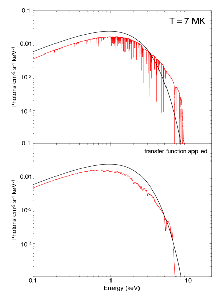
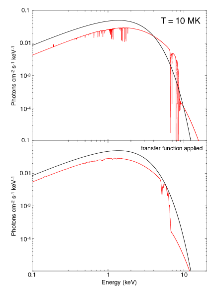
Figure 3: Neutron star atmosphere models with T = $7,10\times 10^{6}$ K. The red curve in the top is the spectrum without the redshift and the broadening effect. The bottom is the spectrum after the transfer function is applied. The black curves are the blackbody spectra with T = $7,10\times 10^{6}$ K.

4 Estimation of the absorption line intensity with Suzaku

4.1 Observations and data reduction

Suzaku observed Serpens X-1 for $\sim 30$ ks on 2006 Oct 24 (Obs. ID : 401048010). The observation of XIS/Suzaku was taken in $\frac{1}{4}$ window with 1 s burst clock mode at the XIS nominal pointing position. We correct the images by using aeattcor2 in the HEAsoft package. The CCD data are still affected by pileup (Yamada et al., 2012), so we remove the data from a circle of radius 60 pixels centered on the brightest pixel, corresponding to a 3% pileup fraction. We sum XIS0, XIS2 and XIS3 using addascaspec in the HEAsoft package and reprocessed HXD PIN data following the standard analysis procedure and adopted ae_hxd_pinxinome3_20080129.rsp as the response file. The non-X-ray background is estimated following the standard analysis thread described on The Suzaku Data Reduction Guide and the cosmic X-ray background is ignored because the source is very bright. The spectra were rebinned so that each bins contain more than 20 counts.

We used XSPEC version 12.9.0 to fit the spectra. The fitting was performed from 1.0 keV to 9.0 keV in the XIS and from 15.0 keV to 20.0 keV in the HXD PIN. The region from 1.5 keV to 2.5 keV was ignored due to the large calibration uncertainties coming from the instrumental edges. We set the normalization of PIN data relative to XIS data as a free parameter. The best fit values of it are consistent with the value (1.16) on The Suzaku Data Reduction Guide in the $\sim 1\sigma$ confidence level (Table 1, 2).

We assumed a neutral hydrogen column density as $4.4\times 10^{21}\mathrm{cm^{-2}}$ (Dickey & Lockman, 1990) via the tbnew_gas model which is a new and improved version of the X-ray absorption model tbabs (Wilms et al., 2000) and set the photoelectric absorption cross-sections as ”vern” and the metal abundances as ”wilm”. Errors in this paper is given at 90% confidence level unless otherwise stated.

4.2 Identification of the spectral components

We fit the spectrum with a continuum model consisting of a disc and Comptonized boundary layer. There is considerable spectral degeneracy in decomposing a broadly curving continuum into two smoothly curving components (e.g. Done et al. 2002; Revnivtsev & Gilfanov 2006), so we use the best physical models for the emission. We describe the disc by the kerrbb model (Li et al., 2005) which includes relativistic smearing of the sum of color temperature corrected blackbody components with luminosity given by the fully relativistic emissivity. We fix the inclination angle of $10^{\circ}$ (Cornelisse et al., 2013) and the mass of 1.4 $\mathrm{M_{\odot}}$ and assume a distance of 10 kpc (the $X=0$ limit from type 1 X-ray burst observations; Galloway et al. 2008). We describe the Comptonisation using the nthcomp model (Zdziarski et al., 1996). This should produce a reflection component from illumination of the disc, but this can be complex (Bhattacharyya & Strohmayer, 2007; Cackett et al., 2008; Miller et al., 2013; Chiang et al., 2016a; Chiang et al., 2016b; Matranga et al., 2017). Here our focus is to describe the continuum shape for a simulation of the narrow redshifted absorption lines, so we simply use a Gaussian emission line to fit the data. The resulting parameters are shown in Table 1.

While the temperature of electrons in the boundary layer, $T_{e}~{}(>3.1\;\mathrm{keV})$ is poorly constrained due to the lack of data in high energy band, the temperature of the surface beneath it, $T_{\mathrm{BL}}~{}(=1.76_{-0.14}^{+0.03}\;\mathrm{keV})$ are close to those derived for the boundary layer in similarly bright LMXB spectra by Revnivtsev & Gilfanov (2006), where they break the spectral degeneracies by Fourier resolved spectroscopy. Thus our spectral decomposition appears reasonable.

The luminosity ratio of the disc emission to the boundary layer emission is $0.943_{-0.029}^{+0.022}$. This potentially already provides some constraints on the EoS modulo neutron star spin (Sibgatullin & Sunyaev, 2000). The boundary layer dissipates the remaining kinetic power of the accretion flow, which will depend on the difference in spin frequency between the disc inner edge and the surface. However, it also depends on the EoS, especially where the neutron star is smaller than the radius of the last stable circular orbit as the boundary layer luminosity is enhanced by the additional kinetic energy of the radially plunging material. The calculations of Sibgatullin & Sunyaev (2000) (their Fig 1) give a spin of 540 Hz for a luminosity ratio of 0.943 with their assumed EoS ($R=11.3$ km for a $1.4~{}M_{\odot}$ neutron star). This is a reasonable spin frequency, but it is probably overestimated as our models for the boundary layer luminosity neglected the reflection continuum.

The expected efficiency of accretion is $\sim 0.14$ (Fig 1 of Sibgatullin & Sunyaev 2000). Combining this with the mass accretion rate through the disc of $0.64\times 10^{18}\;{\mathrm{g/s}}$ (Table 1) gives a total luminosity which is $\sim 45\%$ of the Eddington mass accretion rate for a $1.4~{}M_{\odot}$ neutron star. The total absorption corrected bolometric flux from the data is instead $1.0\times 10^{-8}\;\mathrm{ergs/cm^{2}/s}$, giving a luminosity of $1.2\times 10^{38}\;\mathrm{ergs/s}$ for the assumed distance of 10 kpc, which is $\sim 70\%$ of the the Eddington luminosity. This discrepancy is less than a factor 2, but could indicate either that the distance is $7.7$ kpc, as derived from assuming the solar abundance for the X-ray bursts (Galloway et al., 2008), or that the EoS is different to that assumed in Sibgatullin & Sunyaev (2000).

Componet	Parameter
tbnew_gas	$N_{\mathrm{H}}\;(10^{22}\;\mathrm{cm^{-2}})$	$(0.44)$
kerrbb	$\eta$	(0.0)
	a	(0.2)
	$i$ (deg)	(10.0)
	$M_{\mathrm{bh}}$ ($\mathrm{M_{\odot}}$)	(1.4)
	$M_{\mathrm{dd}}$ ($\mathrm{10^{18}\;g/s}$)	$0.637_{-0.009}^{+0.010}$
	$D_{\mathrm{bh}}$ (kpc)	(10.0)
	hd	$1.653_{-0.019}^{+0.019}$
	rflag	(1.0)
	lflag	(0.0)
	norm	(1.0)
nthComp	Gamma	$6.3_{-3.3}^{+0.3}$
	$kT_{\mathrm{e}}$ (keV)	$>3.1$
	$kT_{\mathrm{bb}}$ (keV)	$1.76_{-0.14}^{+0.03}$
	$L_{\mathrm{disc}}/L_{\mathrm{BL}}$	$0.943_{-0.029}^{+0.022}$
Gaussian	Line E (keV)	$6.656_{-0.031}^{+0.031}$
	$\sigma$ (keV)	$0.233_{-0.036}^{+0.040}$
	norm ($10^{-3}$)	$2.58_{-0.33}^{+0.36}$
constant (HXD PIN)		$1.205_{-0.044}^{+0.045}$
$\chi^{2}/d.o.f.$		2097.5 / 1918

Table 1: Best-fit parameters for kerrbb + nthcomp without the surface blackbody models using Suzaku spectrum

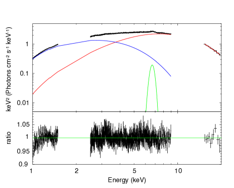
Figure 4: Unfolded Suzaku spectrum with kerrbb + nthcomp without the surface blackbody models. The blue curve is kerrbb, the red one is nthcomp and the green one is Gaussian for the iron line.

4.3 Estimation of the equivalent width of the iron absorption line

We add each of the two different temperature surface spectra described in Section 3 to the emission model derived above. This is the maximum possible contribution from the surface, as it assumes that the entire star is directly visible rather than being partly covered by the boundary layer and partly obscured by the disc. However, these effects are minimized for a pole on view so this represents a reasonable contribution of the surface emission for Serpens X-1. The results are shown in Table 2 and Figure 5. The luminosity of the surface blackbody for the $7\times 10^{6}$ K and $10\times 10^{6}$ K models is 0.8% and 3.3% of the total luminosity respectively, so its inclusion makes a difference in the best-fit continuum parameters. This is most marked for the disc, as the shape of the surface emission overlaps most with this component, so its inclusion reduces the mass accretion rate and $L_{disc}/L_{BL}$.

We use these models to determine the equivalent width of the iron absorption lines from the surface against the brighter continuum emission from the accretion flow. We used fakeit command in XSPEC without errors to produce a model spectrum on a dummy (diagonal) response matrix from 1 keV to 15 keV with energy resolution of 1 eV. We then fit this over the very restricted energy range of 4.7 keV to 5.7 keV with a powerlaw + Gaussian + Gaussian model. A single Gaussian is a good representation of the multiple $n=2~{}\mathchar 45\relax~{}1$ transitions in each ion state as the substructure is blended due to the Doppler shifts (see Section 3). Table 3 shows the resulting equivalent and intrinsic widths. The intrinsic width is higher for the Fe XXV as there is a larger energy range between the multiple transitions (forbidden, intercombination and resonance) than for Fe XXVI (just spin-orbit splitting). Both lines increase in equivalent width for higher temperature, as the contribution of the surface emission increases, but Fe XXV always has higher equivalent width than Fe XXVI, from $0.8~{}\mathchar 45\relax~{}7.7$ eV as the temperature increases from $7~{}\mathchar 45\relax~{}10\times 10^{6}$ K. In the next section, we search the higher resolution Chandra transmission grating data for the absorption lines, and compare the result with these model predictions.

		surface temperature
Componet	Parameter	$7\times 10^{6}$ K	$10\times 10^{6}$ K
kerrbb	$M_{\mathrm{dd}}$ ($\mathrm{10^{18}\;g/s}$)	$0.620_{-0.010}^{+0.010}$	$0.592_{-0.007}^{+0.008}$
	hd	$1.651_{-0.020}^{+0.020}$	$1.601_{-0.015}^{+0.017}$
nthComp	Gamma	$6.2_{-3.3}^{+0.3}$	$6.4_{-3.3}^{+0.4}$
	$kT_{\mathrm{e}}$ (keV)	$>3.0$	$>3.2$
	$kT_{\mathrm{bb}}$ (keV)	$1.75_{-0.15}^{+0.03}$	$1.79_{-0.11}^{+0.03}$
	$L_{\mathrm{disc}}/L_{\mathrm{BL}}$	$0.913_{-0.028}^{+0.029}$	$0.870_{-0.020}^{+0.023}$
Gaussian	Line E (keV)	$6.657_{-0.032}^{+0.030}$	$6.675_{-0.023}^{+0.023}$
	$\sigma$ (keV)	$0.233_{-0.036}^{+0.039}$	$0.244_{-0.027}^{+0.029}$
	norm ($10^{-3}$)	$2.62_{-0.33}^{+0.35}$	$3.43_{-0.33}^{+0.35}$
constant (HXD PIN)		$1.208_{-0.044}^{+0.045}$	$1.16_{-0.041}^{+0.043}$
$\chi^{2}/d.o.f.$		2080.5 / 1918	2131.4 / 1918

Table 2: Best-fit parameters for kerrbb + nthcomp with the surface blackbody models using Suzaku spectrum. $N_{\mathrm{H}}$ is $4.4\times 10^{21}~{}\mathrm{cm^{-2}}$ (fixed).

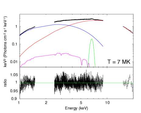
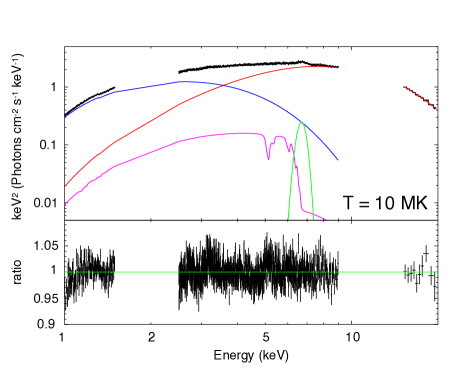
Figure 5: Unfolded Suzaku spectrum with kerrbb + nthcomp with the surface blackbody models. The magenta is the surface model and the blue curve is kerrbb, the red one is nthcomp, the green one is Gaussian for the iron line. The effective temperature of the surface are $7\times 10^{6}~{}\mathrm{K}$ in the left figure and $10\times 10^{6}~{}\mathrm{K}$ in the right one.

	effective temperature	EW(eV)	Energy (keV)	$\sigma$ (eV)
Fe XXV x+y,w,z	$7\times 10^{6}$ K	0.76	5.11	83
Fe XXVI Ly$\alpha$		0.05	5.35	39
Fe XXV x+y,w,z	$10\times 10^{6}$ K	7.7	5.12	86
Fe XXVI Ly$\alpha$		2.0	5.35	53

Table 3: Estimation of the equivalent width of the iron absorption line with different surface temperatures.

5 Line search with Chandra

5.1 Observations and data reduction

Chandra observed Serpens X-1 with the High Energy Transmission Grating Spectrometer (HETGS) twice on 2014 June 27 - 29 and August 25 - 26 (Obs. ID : 16208, 16209) each with $\sim 150$ ks exposure. These data were taken in continuous clocking (CC) mode in which the data are transferred every 2.85 ms in order to avoid pileup. The HETG consists of two sets of gratings, the Medium Energy Grating (MEG) and the High Energy Gratings (HEG) (Canizares et al., 2005). The two gratings have different grating periods, 4001.41 Å in MEG and 2000.81 Å in HEG. Since the MEG’s grating period is almost exactly twice as long as the HEG’s, the scattering angle for the N-th order HEG is very close to that of 2N-th order MEG. The alignment angles for MEG and HEG are very similar ($-5.19^{\circ}$ in HEG and $4.74^{\circ}$ in MEG), so the position along the X-axis of the N-th order HEG and 2N-th order MEG are almost the same as each other.

In the standard (timed exposure: TE) mode, the full imaging is retained, and the MEG and HEG grating orders are separated in Y-axis values as well as X-axis and so do not overlap. However, in CC mode, the information about the position in the columns (CHIPY) is lost because events are read out continuously and the frame image is collapsed into one row. Thus the N-th order HEG and 2N-th order MEG overlap. Normally, in order to avoid this, the source point is placed with a Y-axis offset from the center of the chip so that the MEG positive order and HEG negative order (or MEG negative order and HEG positive order) are excluded from the chips. However, in our data set, the source point is set at the center of the Y axis, so MEG$\pm 2$ are intermixed with HEG$\pm 1$ and the response files (which assume HEG and MEG are separated) are not appropriate. Hence we use only MEG$\pm$1 in our analysis. The MEG effective area is comparable to that of the HEG at 5 keV, so this is not a big loss of signal (see Figure 6).

We processed the data using chandra_repro command in CIAO V4.8 software package and combined data from both observations to produce spectra for MEG+1 and MEG-1 (there are no MEG$\pm 2$ data from this tool due to the overlap with HEG$\pm 1$ discussed above). There is one weak type I burst during the observations, but we did not exclude it because its contributes only $\sim$0.5 % of the total counts (Chiang et al., 2016b). We fixed the hydrogen column density, photoelectric absorption cross-sections and the metal abundances, as for the Suzaku analysis.

5.2 Method of absorption line search

We do a blind search on the Chandra MEG$\pm 1$ data. The target of the search is the combination of Fe XXV x+y, w, z (6.7 keV) since it is the strongest absorption feature in the neutron star atmosphere model over the expected temperature range. We set the range of search redshift as z = 0.1 $\sim$ 0.7, corresponding to an energy for Fe XXV of 6.09 keV to 3.94 keV (though the most likely range of neutron star radii is 10 - 15 km i.e. $z=0.31~{}\mathchar 45\relax~{}0.17$). No discrete structures are seen in the MEG$\pm 1$ effective areas in this range (Figure 6).

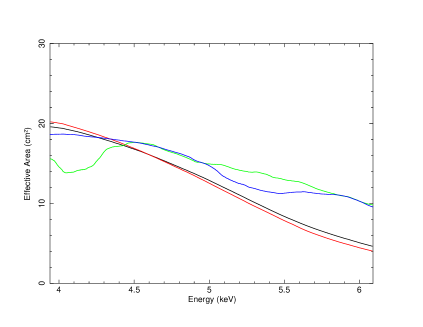
Figure 6: Chandra HETG effective areas. The black curve is MEG-1, the red one is MEG+1, the green one is HEG-1 and the blue one is HEG+1.

We fit the MEG$\pm 1$ spectra separately with separate powerlaw models from 3.90 keV to 6.13 keV (i.e. extended by 0.04 keV from the central energy range so that the line would be fully resolved by the data even at the edge of the redshift range). This adequately describes the continuum over this narrow energy range (see Figure 7). We save the parameters of the best-fit model and the chi-squared values ($\chi^{2}_{0}$). The parameters are not tied between the two spectra as there are differences of a few percent in the flux. This is considered to be due to the scattering halo effect or clocking background which are associated with CC-mode (Schulz, 2014). They do not affect the structure of the absorption line because they make the continuous background. Thus they are of no significance in this analysis.

We fix the power law continuum and add in a Gaussian line, parameterized by the center energy ($E$), standard deviation ($\sigma$) and equivalent width (EW). We fix $\sigma$ at 80 eV (see Table 3) and vary $E$ from 3.94 keV to 6.09 keV in steps of 0.01 keV (much smaller than the expected intrinsic width of the line of 0.08 keV). Thus the only free parameter in the fitting is the EW, which can be either negative or positive, corresponding to absorption and emission lines, respectively. We calculate the difference of the chi-squared values from $\chi^{2}_{0}$ and save it ($\Delta\chi^{2}(E)$) together with the EW of the best-fit model (EW($E$)).

We determine the $3\sigma$ confidence limit on the detection of a line i.e. find the $\Delta\chi^{2}$ which corresponds to a probability of 0.0027 of getting a false positive. This is not straightforward due to the multiple energies searched. We approach this in two different ways. Firstly, we simulate MEG$\pm$1 spectra from a simple powerlaw continuum. We fit these with powerlaw $+$ Gaussian stepping the center energy of the Gaussian over the same energy range as for the real data. We repeat this 10000 times and rank the resulting $\Delta\chi^{2}(E)$, picking the 27th highest (as 10000 $\times$ 0.0027 is 27). This gives $\Delta\chi^{2}_{3\sigma}=15.12$.

We confirm this using a more sophisticated statistical approach from high energy physics, where searching for a signal from a particle of unknown mass is a classic problem (the look elsewhere effect). We follow Gross & Vitells (2010) who show that the relevant $\chi^{2}$ value is that for which

$$\begin{split}P\left(\mathrm{max(\Delta\chi^{2}(E))}>\Delta\chi^{2}_{3\sigma}\right)=\\ P(\chi_{1}^{2}>\Delta\chi^{2}_{3\sigma})&+\langle N(c_{0})\rangle e^{-(c-c_{0})/2}\end{split}$$

where $\chi^{2}_{1}$ is a $\chi^{2}$ distribution with 1 degree of freedom, and $\langle N(c_{0})\rangle$ is the number of ’upcrossings’ between $\Delta\chi^{2}(E)$ and $\Delta\chi^{2}=c_{0}$, that is, the number of $E$ in the search range which satisfies that $\Delta\chi^{2}(E)=c_{0}$ and $\Delta\chi^{2}(E-\epsilon)<c_{0}$ ($\epsilon$ is sufficiently small.). We follow Gross & Vitells (2010) and set $c_{0}=0.5$.

We use the same simulations as before and find $\langle N(c_{0})\rangle=4.42$. This implies $\Delta\chi^{2}_{3\sigma}=15.37$, very similar to the standard simulation result. Hereafter this value is used for the blind search because the first result has a relatively large Poisson error $\sim 0.3$.

5.3 Results of absorption line search

The maximum observed value of $\Delta\chi^{2}(E)$ is 5.41 (upper panel in Figure 8). This is substantially smaller than the value of 15.37 derived above for a $3\sigma$ detection. Therefore we did not find any absorption lines at the 3 $\sigma$ confidence level. The $3\sigma$ upper limit of the equivalent width was found at each energy by increasing the intensity until $\Delta\chi^{2}(E)=15.37$ was reached. These are plotted in the lower panel of Figure 8. The decrease in effective area at higher energies means that this upper limit on any absorption line goes from $-8$ eV for $z=0.1$ to $\sim-2$ eV for $z\geq 0.3$. However, there are broad features present which probably indicate residual continuum curvature which is not well modelled by the assumed power law. A more accurate measure of the upper limit of the line with respect to a more complex continuum is half the difference between the upper and lower limit to EW. This gives $\sim-6,-4,-3,-1.5$ eV at z = 0.1, 0.2, 0.3, 0.7.

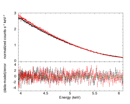
Figure 7: Chandra MEG$\pm 1$ count rate spectrum and the best-fit continuum model. The black curve is MEG-1 and the red one is MEG+1.

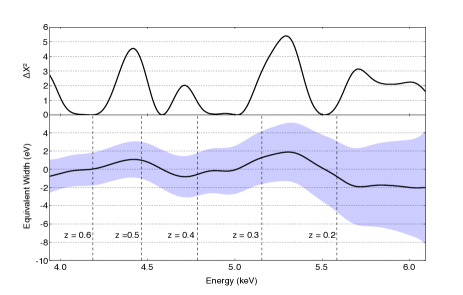
Figure 8: Top: $\Delta\chi^{2}$ at different line energy in the search range. Bottom: Best-fit value of the equivalent width (the black solid line) and $3\sigma$ upper limit of it.

The upper limit from the Chandra data is $-3$ eV at $\sim 5.1$ keV. This rules out an absorption line at $\sim 5.1$ keV with an EW as large as $7.7$ eV as predicted by the $10\times 10^{6}$ K surface model. It is instead consistent with the predicted absorption line EW of 0.8 eV for the lower surface temperature of $7\times 10^{6}$ K. We simulated this photosphere model through the Chandra response using the fakeit command, and estimate that such a line could be detected at the $3\sigma$ confidence level with a 3 - 4 Ms exposure.

6 Discussion

The Chandra data clearly show that either the neutron star surface temperature is lower than $10\times 10^{6}$ K or some other mechanism suppresses the absorption line. We first assess the expected surface temperature, and then examine the other assumptions which determine the absorption line strength.

6.1 Surface temperature

We measured the surface temperature beneath the boundary layer as $\sim$ 1.7 keV from the seed photon energy of the Comptonization component in the broadband Suzaku data (Table 1). However the temperature at the pole is not necessarily the same. The equator is illuminated by the boundary layer and subject to ram pressure heating, whereas the pole is largely unaffected by these. Instead, the pole is heated by thermal conduction from the equator and from the interior of the star (though this is probably negligible in comparison).

We calculate the distribution of the temperature on the surface solving the heat equation. We assume the spherical crust of the neutron star with a thickness of $h$. In spherical coordinates, it is described as:

$$\begin{split}\rho C_{p}\frac{\partial T}{\partial t}=\frac{1}{r^{2}}\frac{\partial}{\partial r}\left(\kappa r^{2}\frac{\partial T}{\partial r}\right)+\frac{1}{r^{2}\sin\theta}\frac{\partial}{\partial\theta}\left(\kappa\sin\theta\frac{\partial T}{\partial\theta}\right)\\ +\frac{1}{r^{2}\sin^{2}\theta}\frac{\partial}{\partial\phi}\left(\kappa\frac{\partial T}{\partial\phi}\right)+g\end{split}$$

$\rho$ is the mass density and $C_{p}$ is the heat capacity and $\kappa$ is the thermal conductivity and $g$ represents external sources. Assuming that $\frac{\partial T}{\partial t}=0$ and $\kappa$ is constant in the crust, and ignoring $r$- and $\phi$- dependence for simplicity, the heat equation becomes:

$$0 = \frac{\kappa}{R^{2}\sin\theta}\frac{\mathrm{d}}{\mathrm{d}\theta}\left(\sin\theta\frac{\mathrm{d}T_{\theta}}{\mathrm{d}\theta}\right)+g$$

$$= \frac{\kappa}{R^{2}}\frac{\mathrm{d}}{\mathrm{d}\left(\cos\theta\right)}\left(\left(1-\cos^{2}\theta\right)\frac{\mathrm{d}}{\mathrm{d}\left(\cos\theta\right)}\right)T_{\theta}+g$$

$R$ is the radius of the neutron star. When we integrate this equation along the $r$-axis from the inner crust ($r=R-h$) to the outer crust ($r=R$), the external sources are a black body radiation from the surface and the heat transfer from the neutron star core. Thus the heat equation in a spherical shell at latitude $\theta$ (measured from the pole, so $\theta=\pi/2$ corresponds to the equator) is

$$\sigma_{s}T_{\theta}^{4} = \frac{\kappa h}{R^{2}}\frac{\mathrm{d}}{\mathrm{d}\left(\cos\theta\right)}\left(\left(1-\cos^{2}\theta\right)\frac{\mathrm{d}}{\mathrm{d}\left(\cos\theta\right)}\right)T_{\theta}+Q$$

where $Q$ is the heat energy from the interior of the star.

We assume $Q=0$ for simplicity and set the boundary conditions as $T_{\theta=\pi/2}=T_{0}$ and

$$\frac{R^{2}\sigma_{s}}{\kappa h}T_{\theta}^{4}+2\frac{\mathrm{d}T_{\theta}}{\mathrm{d}(\cos\theta)}=0\;(\mathrm{at}~{}\theta=0)$$

The latter equation represents non-divergence of second-order differentiation of $T$ at the pole. The thermal conductivity $\kappa$ in the crust is from $10^{18}$ to $10^{24}$ erg cm^-1 K^-1 s^-1 depending on the density and magnetic field (Geppert et al., 2004). Figure 9 shows the thermal distribution when we set $T_{0}$ and $\kappa$ to be 1.7 keV and $10^{23}$ erg cm^-1 K^-1 s^-1. We assume $h=10^{5}~{}\mathrm{cm}$ and $R=10^{6}~{}\mathrm{cm}$. This gives a temperature at the pole of $\sim 5.6\times 10^{6}$ K.

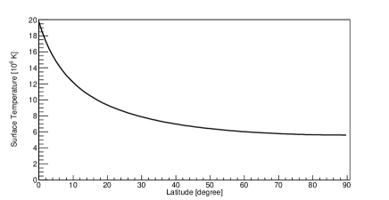
Figure 9: Thermal distribution along the latitude. We set $T_{0}$ as $1.7$ keV and $\kappa$ as $10^{23}\;\mathrm{erg\;cm^{-1}\;K^{-1}\;s^{-1}}$.

Observationally we see the angle averaged surface temperature. We define $T_{\mathrm{ave}}$ defined by

$$\sigma_{s}T_{\mathrm{ave}}^{4}\pi R^{2} = \int_{0}^{\frac{\pi}{2}}\sigma_{s}T_{\theta}^{4}2\pi R^{2}\sin\theta\cos\theta\mathrm{d}\theta$$

as the average of the blackbody radiation ($\sigma_{s}T_{\theta}^{4}$) over the surface. It is $\sim 8\times 10^{6}$ K for the model shown in Figure 9. This temperature is close to that of the lower temperature simulation, so predicts a line EW of a few eV, consistent with the limit from the Chandra data. However, it is more likely that $\kappa$ is lower. Rutledge et al. (2002) discuss the crustal conductivity calculated from from electron-ion (appropriate for the envelope) and electron-phonon scattering (as appropriate for the crystalline phase, see also Potekhin et al. 2015). This gives $\kappa=10^{19-20}$ erg cm^-1 K^-1 s^-1, consistent with observations of neutron star cooling after a transient accretion episode (Rutledge et al., 2002). Figure 10 shows the dependence of $T_{\mathrm{ave}}$ on $\kappa$. For such low values of the thermal conductivity, the angle averaged temperature is $\sim 1~{}\mathchar 45\relax~{}2\times 10^{6}$ K and a very little absorption line is produced. In addition, the distribution of the iron ionization state becomes so complex that the line identification is too complicated even if it is observed (Figure 2).

These low temperatures are very close to the temperatures observed for the neutron star surface cooling after a transient accretion episode (Heinke, 2013; Degenaar et al., 2015). This emission is powered by deep crustal heating by pycnonuclear reactions during accretion, and sets a lower limit to the temperature of the pole even when thermal conductivity is low. This points to the need for more sophisticated calculations which include the energy exchanged with the inner part of the star. Nonetheless, it appears feasible that the surface temperature of the neutron star surface near the pole is less than $7\times 10^{6}$ K and so produces an Fe XXV absorption line EW which is less than 1 eV, undetectable with current data. However, there are other possible issues which could suppress the line EW. We explore them below.

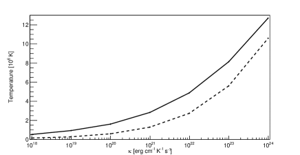
Figure 10: Dependence of the surface temperature on $\kappa$ : The solid line is the temperature averaged over the surface, $T_{\mathrm{ave}}$. The dashed line is the temperature at the pole, $T_{\theta=0}$. The range of $\kappa$ is derived from Geppert et al. (2004).

6.2 Uncovered surface area and metallicity

The disc accretion onto the neutron star surface terminates in a boundary layer, where the deceleration takes place in an equatorial belt with meridional extent set by the mass accretion rate (Inogamov & Sunyaev, 1999). The boundary layer is optically thick, so shields the surface from view, and is hot enough that iron should be completely ionized so it produces no atomic features. The extent of the boundary layer depends on mass accretion rate, and for the $0.3~{}\mathchar 45\relax~{}0.6~{}L_{\mathrm{Edd}}$ (distance of 7.7 - 10 kpc) derived for Serpens X-1 in Section 4, the accretion belt will cover around half of the visible neutron star surface. This will halve the predicted line EW for a given temperature, but a surface as hot as $10^{7}$ K would still be marginally inconsistent with the Chandra upper limits for a 10-13 km neutron star. However, the geometry of the boundary layer also depends on other physical parameters. For example, in the case that the disc thickness on the neutron star surface is relatively thick, the boundary layer can reach the pole if $L_{\mathrm{BL}}>0.25~{}\mathchar 45\relax~{}0.4~{}L_{\mathrm{Edd}}$ (Suleimanov & Poutanen, 2006). Thus we cannot rule out the possibility that the neutron star surface is totally covered by the optically thick corona.

The extent of the boundary layer also determines the metallicity of the photosphere at the pole. Heavy metals sink on a timescale of $\sim 10$ s due to the strong gravity of the neutron star (Bildsten et al., 2003), but even low levels of accretion are sufficient to replenish iron in the photosphere (Özel, 2013). The meridional structure of the boundary layer means that the deposition of fresh material takes place in the equatorial belt rather than at the pole. Hence it is possible that there is an abundance gradient with polar angle, with the pole being mostly Hydrogen while the metals are confined to the hot boundary layer. This anti-correlation of metallicity with ’bare’ (uncovered by the boundary layer) neutron star surface would mean that no iron absorption lines could be seen whatever the polar temperature. However, the amount of accretion required to replenish the photosphere is very small, and the maximum polar angle extent of the boundary layer is not sharp. There is a ’dark layer’ of material beyond the bright boundary layer which extends closer towards the poles, especially for the fairly high accretion rates considered here (Inogamov & Sunyaev, 1999), so it seems unlikely that metals are absent from the surface.

6.3 Boundary layer illumination of atmosphere

The model atmosphere calculations in Section 3 assume that there is no additional heating from illumination. Plainly the boundary layer will illuminate the surface at the pole to some extent, though the equatorial belt geometry means that only a small fraction of the boundary layer flux will be intercepted by the polar regions. While this could contribute to heating the surface, increasing the expected absorption line depth, irradiation can produce a temperature inversion which switches the line into emission. There are no current calculations of this effect, but we note that our Chandra upper limits are equally stringent for emission as for absorption.

6.4 Inclination offset and spin frequency

The binary inclination is small, $\sim 10^{\circ}$ (Cornelisse et al., 2013), but the neutron star spin axis could be misaligned from the binary orbit due to the supernovae kick at its formation (Brandt & Podsiadlowski, 1995). This leads to both misalignment of the spin and orbit, and high orbital eccentricity but both of these are removed by tidal forces, often before the companion fills its Roche lobe and the system becomes an LMXB (Hut, 1981). Thus the neutron star spin in Serpens X-1 should be aligned with the binary orbit, and the binary orbit inclination is low (Cornelisse et al., 2013). However, measurements of the inclination from sophisticated fitting of the reflected signature from the boundary layer illumination of the accretion disc gives a significantly larger value, $i\sim 27^{\circ}$ (Matranga et al., 2017), which would be sufficient to broaden the line beyond detectability as a narrow feature. Inclination is difficult to measure precisely by reflection, as it depends on the spectral modelling (compare to Miller et al. 2013 who used less physical models but derived $i\sim 9^{\circ}$ from the same data). We conclude that the inclination angle to the neutron star spin axis is most likely low, so this is not the origin of the loss of narrow line.

The spin frequency of Serpens X-1 has not been detected. In our model prediction, we assume that it is 400 Hz. This is a typical value in observed LMXBs (Altamirano et al., 2012; Patruno & Watts, 2012). In the spectral analysis in Section 4.2, the spin frequency is estimated as $\sim$ 500 Hz using the luminosity ratio of the disc emission to the boundary layer emission, and it is consistent with that of LMXBs. However if this object is a peculiar source and the spin frequency is over than $\sim$ 1 kHz, the absorption lines would be totally broadened.

7 Conclusions

We show that atomic features from highly ionized iron are potentially observable in the persistent (non burst) emission of accreting LMXB for low inclination or low spin neutron stars. Serpens X-1 is the only known non-transient system which fulfils these constraints, having low orbital inclination. This is on the middle banana branch, so the accretion flow geometry is probably an accretion disc which forms a boundary layer around the neutron star equator, leaving the polar surface directly visible. We use the Suzaku broadband data to model the continuum emission, and then use this as a baseline to add in the predicted surface emission. We model this for two temperatures which span a reasonable range for the polar surface of $7~{}\mathchar 45\relax~{}10\times 10^{6}$ K. These predict an absorption line from Fe XXV K$\alpha$ with equivalent width of 0.8 - 8 eV for a completely equatorial boundary layer, or 0.4 - 4 eV if the boundary layer covers half of the neutron star surface. We search for this line in existing Chandra grating data, and find an upper limit of 2 - 3 eV. We discuss potential reasons for this non-detection (the surface temperature, the geometry of the boundary layer, the metallicity in the atmosphere, the inclination angle and the spin frequency of the star). Our conclusion is that the line is likely there at the level of 1eV, a combination of the boundary layer obscuring half of the surface, and the polar temperature being lower than $10\times 10^{6}$ K. However, to detect such a line at $3\sigma$ confidence would require 3-4 Ms exposure time with the Chandra gratings. Thus it is unlikely that current instrumentation can obtain substantially better constraints. The effective area of XARM (the Hitomi recovery mission) is $\sim$ 10 times as large as that of Chandra around 5 keV, so the line could be detected at $3\sigma$ confidence in $\sim$ 300 ks. The future X-ray mission Athena has a much larger effective area (Figure 4 in Barret et al. 2013), so should be able to constrain such a small EW with an observation of around $2\times 10^{4}$ s. The potential of such future observations motivates more theoretical work on the neutron star surface emission (including a two dimensional analysis of the temperature, abundances and effect of illumination) in order to obtain a better understanding of the expected features.

Appendix A MEG$\pm$1 and HEG$\pm$1

Just for reference, we show the result in Figure 11, 12 when HEG$\pm$1 data are included to the analysis. We obtained $\langle N(0.5)\rangle=4.20$ and ${\Delta\chi^{2}_{\mathrm{3\sigma}}}=15.27$. (The number of trials of Section 5.2 (iii) is 1000.) As shown in Figure 11, the HEG+1 spectrum is rolling and the powerlaw model does not fit it well. Due to this, a large $\Delta\chi^{2}$ is seen in Figure 12 around 4.7 keV where the residuals is significant in HEG+1. Therefore the $\Delta\chi^{2}$ around 4.7 keV is larger than $\Delta\chi^{2}_{\mathrm{3\sigma}}$ but this does not mean that we have detected the absorption line. Considering that the other spectra are fitted well simply with the powerlaw model, it is natural that the spectrum data or the response file are not correct due to the mixing. If we use the response file which consider that the HEG+1 spectrum is intermixed with the MEG+2, the matters might be improved.

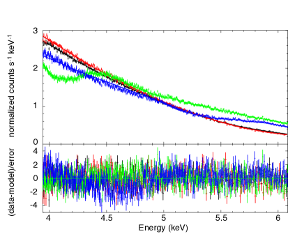
Figure 11: Chandra MEG$\pm 1$ & HEG$\pm$1 count rate spectrum and the best-fit continuum model. The black curve is MEG-1, the red one is MEG+1, the green one is HEG-1 and the blue one is HEG+1.

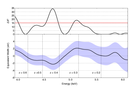
Figure 12: Top: $\Delta\chi^{2}$ at different line energy in the search range. Bottom: Best-fit value of the equivalent width (the black solid line) and $3\sigma$ upper limit of it. The red line represents for 3 $\sigma$ detection level (${\Delta\chi^{2}_{\mathrm{3\sigma}}}=15.27$).

References

- Altamirano et al. (2012) Altamirano D., Ingram A., van der Klis M., Wijnands R., Linares M., Homan J., 2012, ApJ, 759, L20
- Antoniadis et al. (2013) Antoniadis J., et al., 2013, Science, 340, 448
- Barret et al. (2013) Barret D., et al., 2013, in Cambresy L., Martins F., Nuss E., Palacios A., eds, SF2A-2013: Proceedings of the Annual meeting of the French Society of Astronomy and Astrophysics. pp 447–453 (arXiv:1310.3814)
- Bauböck et al. (2013) Bauböck M., Psaltis D., Özel F., 2013, ApJ, 766, 87
- Bhattacharyya & Strohmayer (2007) Bhattacharyya S., Strohmayer T. E., 2007, ApJ, 664, L103
- Bildsten et al. (2003) Bildsten L., Chang P., Paerels F., 2003, ApJ, 591, L29
- Brandt & Podsiadlowski (1995) Brandt N., Podsiadlowski P., 1995, MNRAS, 274, 461
- Cackett et al. (2008) Cackett E. M., et al., 2008, ApJ, 674, 415
- Canizares et al. (2005) Canizares C. R., et al., 2005, PASP, 117, 1144
- Chang et al. (2005) Chang P., Bildsten L., Wasserman I., 2005, ApJ, 629, 998
- Chiang et al. (2016a) Chiang C.-Y., Morgan R. A., Cackett E. M., Miller J. M., Bhattacharyya S., Strohmayer T. E., 2016a, preprint, (arXiv:1604.08626)
- Chiang et al. (2016b) Chiang C.-Y., et al., 2016b, The Astrophysical Journal, 821, 105
- Cornelisse et al. (2013) Cornelisse R., Casares J., Charles P. A., Steeghs D., 2013, MNRAS, 432, 1361
- Cottam et al. (2002) Cottam J., Paerels F., Mendez M., 2002, Nature, 420, 51
- Cottam et al. (2008) Cottam J., Paerels F., Méndez M., Boirin L., Lewin W. H. G., Kuulkers E., Miller J. M., 2008, ApJ, 672, 504
- Degenaar et al. (2015) Degenaar N., et al., 2015, MNRAS, 451, 2071
- Demorest et al. (2010) Demorest P. B., Pennucci T., Ransom S. M., Roberts M. S. E., Hessels J. W. T., 2010, Nature, 467, 1081
- Di Salvo et al. (2015) Di Salvo T., et al., 2015, MNRAS, 449, 2794
- Dickey & Lockman (1990) Dickey J. M., Lockman F. J., 1990, ARA&A, 28, 215
- Done et al. (2002) Done C., Życki P. T., Smith D. A., 2002, MNRAS, 331, 453
- Done et al. (2007) Done C., Gierliński M., Kubota A., 2007, A&ARv, 15, 1
- Done et al. (2014) Done C., et al., 2014, preprint, (arXiv:1412.1164)
- Galloway et al. (2008) Galloway D. K., Muno M. P., Hartman J. M., Psaltis D., Chakrabarty D., 2008, ApJS, 179, 360
- Galloway et al. (2010) Galloway D. K., Lin J., Chakrabarty D., Hartman J. M., 2010, ApJ, 711, L148
- Geppert et al. (2004) Geppert U., Küker M., Page D., 2004, A&A, 426, 267
- Gierliński & Done (2002) Gierliński M., Done C., 2002, MNRAS, 337, 1373
- Gross & Vitells (2010) Gross E., Vitells O., 2010, European Physical Journal C, 70, 525
- Heinke (2013) Heinke C. O., 2013, in Journal of Physics Conference Series. p. 012001 (arXiv:1303.0317), doi:10.1088/1742-6596/432/1/012001
- Hut (1981) Hut P., 1981, A&A, 99, 126
- Inogamov & Sunyaev (1999) Inogamov N. A., Sunyaev R. A., 1999, Astronomy Letters, 25, 269
- Kajava et al. (2014) Kajava J. J. E., et al., 2014, MNRAS, 445, 4218
- Lattimer (2012) Lattimer J. M., 2012, Annual Review of Nuclear and Particle Science, 62, 485
- Li et al. (2005) Li L.-X., Zimmerman E. R., Narayan R., McClintock J. E., 2005, ApJS, 157, 335
- Loeb (2003) Loeb A., 2003, Physical Review Letters, 91, 071103
- Matranga et al. (2017) Matranga M., Di Salvo T., Iaria R., Gambino A. F., Burderi L., Riggio A., Sanna A., 2017, A&A, 600, A24
- Medvedev & Narayan (2001) Medvedev M. V., Narayan R., 2001, ApJ, 554, 1255
- Miller & Lamb (2016) Miller M. C., Lamb F. K., 2016, European Physical Journal A, 52, 63
- Miller et al. (2013) Miller J. M., et al., 2013, ApJ, 779, L2
- Oosterbroek et al. (2001) Oosterbroek T., Barret D., Guainazzi M., Ford E. C., 2001, A&A, 366, 138
- Özel (2013) Özel F., 2013, Reports on Progress in Physics, 76, 016901
- Özel & Freire (2016) Özel F., Freire P., 2016, ARA&A, 54, 401
- Patruno & Watts (2012) Patruno A., Watts A. L., 2012, preprint, (arXiv:1206.2727)
- Potekhin et al. (2015) Potekhin A. Y., Pons J. A., Page D., 2015, Space Sci. Rev., 191, 239
- Rauch et al. (2008) Rauch T., Suleimanov V., Werner K., 2008, A&A, 490, 1127
- Revnivtsev & Gilfanov (2006) Revnivtsev M. G., Gilfanov M. R., 2006, A&A, 453, 253
- Revnivtsev et al. (2013) Revnivtsev M. G., Suleimanov V. F., Poutanen J., 2013, MNRAS, 434, 2355
- Rutledge et al. (2002) Rutledge R. E., Bildsten L., Brown E. F., Pavlov G. G., Zavlin V. E., Ushomirsky G., 2002, ApJ, 580, 413
- Sakurai et al. (2014) Sakurai S., et al., 2014, PASJ, 66, 10
- Schulz (2014) Schulz N., 2014, Technical report, Calibration Properties of CHANDRA HETG Spectra Observed in CC-Mode, Version 3.0. The Chandra X-Ray Center
- Sibgatullin & Sunyaev (2000) Sibgatullin N. R., Sunyaev R. A., 2000, Astronomy Letters, 26, 699
- Suleimanov & Poutanen (2006) Suleimanov V., Poutanen J., 2006, MNRAS, 369, 2036
- Whittenbury et al. (2014) Whittenbury D. L., Carroll J. D., Thomas A. W., Tsushima K., Stone J. R., 2014, Phys. Rev. C, 89, 065801
- Wilms et al. (2000) Wilms J., Allen A., McCray R., 2000, ApJ, 542, 914
- Yamada et al. (2012) Yamada S., et al., 2012, PASJ, 64, 53
- Zdziarski et al. (1996) Zdziarski A. A., Johnson W. N., Magdziarz P., 1996, MNRAS, 283, 193