Our goal in this section is to prove an upper bound on the roots of the mixed characteristic polynomial $\mixed{A_{1},\dots,A_{m}}{x}$ as a function of the $A_{i}$, in the case of interest $\sum_{i=1}^{m}A_{i}=I$. Our main theorem is:

Theorem 0.1.

Let $A_{1},\ldots,A_{m}$ be positive semidefinite Hermitian matrices satisfying

$$\sum_{i=1}^{m}A_{i}=I\and\trace{A_{i}}\leq\epsilon$$

for all $i$. Then the largest root of $\mixed{A_{1},\ldots,A_{m}}{x}$ is at most $(1+\sqrt{\epsilon})^{2}$.

We begin by performing a simple but useful change of variables that will allow us to reason separately about the effect of each $A_{i}$ on the roots of $\mixed{A_{1},\ldots,A_{m}}{x}$.

Lemma 0.2.

Let $A_{1},\dots,A_{m}$ be Hermitian positive semidefinite matrices. If $\sum_{i}A_{i}=I$, then

$$\mixed{A_{1},\dots,A_{m}}{x}=\left(\prod_{i=1}^{m}1-\partial_{y_{i}}\right)\mydet{\sum_{i=1}^{m}y_{i}A_{i}}\Big{|}_{y_{1}=\dots=y_{m}=x}.$$ (1)

Proof 0.3.

For any differentiable function $f$, we have

$$\partial_{y_{i}}(f(y_{i}))\big{|}_{y_{i}=z_{i}+x}=\partial_{z_{i}}f(z_{i}+x).$$

So, the lemma follows by substituting $y_{i}=z_{i}+x$ into the expression eqn:mixed2, and observing that it produces the expression on the right hand side of eqn:mixed1.

Let us write

$$\mixed{A_{1},\ldots,A_{m}}{x}=Q(x,x,\ldots,x),$$ (2)

where $Q(y_{1},\ldots,y_{m})$ is the multivariate polynomial on the right hand side of eqn:mixed2. The bound on the roots of $\mixed{A_{1},\ldots,A_{m}}{x}$ will follow from a “multivariate upper bound” on the roots of $Q$, defined as follows.

Definition 0.4.

Let $p(z_{1},\ldots,z_{m})$ be a multivariate polynomial. We say that $z\in\R^{m}$ is above the roots of $p$ if

$$p(z+t)>0\qquad\textrm{for all}\qquad t=(t_{1},\ldots,t_{m})\in\R^{m},t_{i}\geq 0,$$

i.e., if $p$ is positive on the nonnegative orthant with origin at $z$.

We will denote the set of points which are above the roots of $p$ by $\above 0.0pt{p}$ (for convenience, we will say that $\above 0.0pt{0}=\R^{m}$). A simple lemma we will find useful is that the region above the roots of $p$ never shrinks under the operation of partial differentiation.

Lemma 0.5.

For any real stable polynomial $p$, $\above 0.0pt{p}\subseteq\above 0.0pt{p_{z_{i}}}$.

To prove Theorem 0.1, it is sufficient by eqn:plugq to show that $(1+\sqrt{\epsilon})^{2}\cdot\bvec{1}\in\above 0.0pt{Q}$, where $\bvec{1}$ is the all-ones vector. We will achieve this by an inductive “barrier function” argument. In particular, we will construct $Q$ iteratively via a sequence of operations of the form $(1-\partial_{y_{i}})$, and we will track the locations of the roots of the polynomials that arise in this process by studying the evolution of the functions defined below.

Our procedure will be to transform the real stable polynomial

$$p(z_{1},\dots,z_{n})=\mydet{z_{i}\sum_{i}A_{i}}$$

into

$$p_{n}(x)=\prod_{i}(1-\partial_{i})\mydet{z_{i}\sum_{i}A_{i}}$$

iteratively, keeping track of what happens to the points above the roots of $p$. At the beginning, the region above the roots will be the positive orthant (since the $A_{i}$ are all positive semidefinite). At step $k$, we will performing the $(1-\partial_{k})$ operation to the polynomial, which (for lack of a better analogy) one can think of as a hitting a metal cast of the “above the roots” region with a hammer. In particular, it will do two things:

1. Shift the entire region in the $z_{k}$ direction

2. Cause the region to flatten inwards (in all directions)

Both effects will cause the zeros of the polynomial to move away from the origin, but the goal will be to bound the amount of movement. Our method of obtaining such a bound uses a collection of measurements that tell us how convex the polynomial is at a given point, in a given variable. We call these measurements “barrier functions” and we will need one such measurement for each variable in $p$.

Definition 0.6.

Given a real stable polynomial $p$ and a point $z=(z_{1},\ldots,z_{m})\in\above 0.0pt{p}$, the barrier function of $p$ in direction $i$ at $z$ is defined as

$$\Phi^{i}_{p}(z)=\frac{\partial_{z_{i}}p(z)}{p(z)}.$$

Equivalently, we may define $\Phi^{i}_{p}$ as

$$\Phi^{i}_{p}(z_{1},\ldots,z_{m}):=\frac{q_{z,i}^{\prime}(z_{i})}{q_{z,i}(z_{i})}=\sum_{j=1}^{r}\frac{1}{z_{i}-\lambda_{j}},$$ (3)

where the univariate restriction

$$q_{z,i}(t):=p(z_{1},\ldots,z_{i-1},t,z_{i+1},\ldots,z_{m})$$ (4)

has roots $\lambda_{1},\ldots,\lambda_{r}$ (which are all real, by Proposition LABEL:prop:setreal).

Note that the barrier functions are (for general points) not particularly well behaved, but we will only be considering them on the set of points that are above the roots, where they have a number of nice properties that we will exploit. Of course applying the $(1-\partial_{k})$ operation will have an effect on the values of the barrier functions, and so we will need to mindful of this change as well. One observation that will simplify this is that the effect of applying $(1-\partial_{k})$ to the barrier function $\Phi^{j}$ can be calculated with all of the other variables (not $z_{k}$ or $z_{j}$) fixed. Hence it suffices to understand the effects on bivariate polynomials, an example of which is shown in Figure 1.

(pic) at (0, 0) ; (legend) at (3.5, 3.5) blue - - $p(x,y)=0$ red - - $\Phi^{x}_{p}(x,y)=0.8$ green - - $\Phi^{y}_{p}(x,y)=0.8$ blue — $q(x,y)=0$ red — $\Phi^{x}_{q}(x,y)=0.8$ green — $\Phi^{y}_{q}(x,y)=0.8$ ;

Figure 1: The effect of the $(1-\partial_{y})$ operator on the bivariate real stable polynomial $p(x,y)=4+12x+8x^{2}+17y+29xy+8x^{2}y+14y^{2}+13xy^{2}+y^{3}$. Note $q(x,y)=(1-\partial_{y})p(x,y)$.

Our proof of these will use an an observation of Terry Tao that uses a characterization of interlacing polynomials that appears in [wagner].

Lemma 0.7.

Let $f$ and $g$ be real rooted polynomials with leading coefficient having the same sign such that $f\ll g$. Then

$$(-1)^{k}\frac{\partial^{k}}{(\partial x)^{k}}\frac{f(x)}{g(x)}\bigg{|}_{x=y}\geq 0$$

for all $y\in\above 0.0pt{g}$.

Proof 0.8.

Let $\beta_{1},\dots\beta_{n}$ be the roots of $g$. Note that the equation

$$f(x)=g(x)\left(s+\sum_{i}\frac{t_{i}}{x-\beta_{i}}\right)$$

defines $n+1$ linearly independent equations in $n+1$ variables (one for each coefficient) and therefore has a solution. Furthermore, one can check that each $t_{i}$ is nonnegative by noting that $f(\beta_{i})=t_{i}g^{\prime}(\beta_{i})$ and using the fact that both $f(\beta_{i})$ and $g^{\prime}(\beta_{i})$ alternate between nonpositive and nonnegative values (the first is due to the interlacing, the second is always true). The result then follows by taking the derivatives and using the fact that $y-\beta_{i}>0$ for all $i$.

Using this, we can show the two analytic properties of barrier functions that we need: at any point above the roots of a real stable polynomial, the barrier functions are nonincreasing and convex in every coordinate.

Lemma 0.9.

Suppose $p$ is real stable and $z\in\above 0.0pt{p}$. Then for all $i,j\leq m$ and $\delta\geq 0$,

$$\Phi^{i}_{p}(z+\delta e_{j}) \leq\Phi^{i}_{p}(z),\text{ and}\qquad$$ (monotonicity) (5)

$$\Phi^{i}_{p}(z+\delta e_{j}) \leq\Phi^{i}_{p}(z)+\delta\cdot\partial_{z_{j}}\Phi^{i}_{p}(z+\delta e_{j})$$ (convexity). (6)

Proof 0.10.

If $i=j$ then consider the real-rooted univariate restriction $q(x_{i})=\prod_{k=1}^{r}(x_{i}-\lambda_{k})$ defined in eqn:restrictdef. Since $z\in\above 0.0pt{p}$ we know that $z_{i}>\lambda_{k}$ for all $k$. Monotonicity follows immediately by considering each term in eqn:concdef, and convexity is easily established by computing

$$\partial^{2}_{x_{i}}\left(\frac{1}{x_{i}-\lambda_{k}}\right)\bigg{|}_{x=z}\frac{2}{(z_{i}-\lambda_{k})^{3}}$$

which is positive since (for $z\in\above 0.0pt{p}$) $z_{i}>\lambda_{k}$. For the case when $i\neq j$, we fix all variables other than $x_{i}$ and $x_{j}$ and consider the bivariate restriction

$$q(x_{i},x_{j}):=p(z_{1},\dots,x_{i},\dots,x_{j},\dots,z_{m}).$$

Using Lemma 0.7, both monotonicity and convexity would follow by showing that $f\ll g$ where

$$f(x_{j}):=\partial_{x_{i}}q(z_{i},x_{j})\and g(x_{j}):=q(z_{i},x_{j})$$

By Corollary LABEL:cor:partialRealStable, $(1+\lambda\partial_{x_{i}})q$ is real stable (and so $g+\lambda f$ is real rooted) for all $\lambda$. Hence by Theorem LABEL:thm:HKO either $f\ll g$ or $g\ll f$.

To show that, in fact, $f\ll g$, we will consider the sum of the roots. That is, it suffices to show that the sum of the roots of $f$ is at most the sum of the roots of $g$. Write

$$q(x,y)=a(y)x^{n}+b(y)x^{n-1}+\dots$$

Since taking partial derivatives preserves real stability,

$$\partial_{x}^{n-1}q(x,y)=(n-1)!(nxa(y)+b(y))$$

is real stable. Hence $b(y)+ia(y)$ is stable and so by Theorem LABEL:thm:HB, we have $a\ll b$. Using Lemma 0.7 again, this implies $a(y)b^{\prime}(y)-b(y)a^{\prime}(y)\geq 0$.

Now since $(x,y)$ is above the roots of $q$, it is also above the roots of $\partial_{x}^{n}q(x,y)=n!a(y)$ and so $a^{\prime}(y)$ and $a(y)$ have the same sign. Hence

$$\frac{b^{\prime}(y)}{a^{\prime}(y)}\geq\frac{b(y)}{a(y)}$$ (7)

Note that the sum of the roots of $g$ is $-b/a$ and the sum of the roots of $f$ is $-b^{\prime}/a^{\prime}$. Thus (7) is asserting that the sum of the roots of $f$ is at most the sum of the roots of $g$ (as needed).

Remark 0.11.

Our original proof of monotonicity and convexity used a powerful characterization of bivariate real stable polynomials due to Helton and Vinnikov [HeltonVinnikov] and Lewis, Parrilo and Ramana [lax]. While this characterization is extremely useful, it (incorrectly) gave the the impression that such a powerful result was required to prove Lemma 0.9. James Renegar, in particular, pointed out that the lemma follows directly from well-known properties of hyperbolic polynomials. We chose the proof given here since it has the benefit of remaining in the domain of real stable polynomials.

Our first observation is that when a point above the roots has a small enough boundary function in a given direction, it remains above the roots after applying an operator in that direction. Pictorially, this asserts that the dotted green line in Figure 1 will always be contained inside the solid blue line.

Lemma 0.12.

Let $p$ be a real stable polynomial, and let $z$ be a point above the roots of $p$ which satisfies $\Phi_{p}^{i}(z)<1$. Then $z$ is also above the roots of $p-\partial_{z_{i}}p$.

Proof 0.13.

Let $t$ be a nonnegative vector. As $\Phi$ is nonincreasing in each coordinate we have $\Phi_{p}^{i}(z+t)<1$, whence

$$\partial_{z_{i}}p(z+t)<p(z+t)\implies(p-\partial_{z_{i}}p)(x+t)>0,$$

as desired.

While Lemma 0.12 proves what we need for a single iteration, it is not strong enough for an inductive argument because the application of a $(1-\partial_{z_{k}})$ operator will typically cause all of the barrier functions to increase. As previously mentioned, the effect of the $(1-\partial_{z_{k}})$ operator will be to shift in the $z_{k}$ direction and flatten away from the origin. To remedy this, we will translate our upper bounds in the $z_{k}$ direction as well (see Figure 2). Certainly this will compensate for the shift in the $z_{k}$ direction, but we will need to move extra in order to compensate for the flattening of the region. How much extra will be determined by the value of the barrier function in that direction. In particular, by exploiting the convexity properties of the $\Phi_{p}^{i}$, we arrive at the following useful strengthening of Lemma 0.12.

Lemma 0.14.

Suppose $p(z_{1},\ldots,z_{m})$ is real stable with $z\in\above 0.0pt{p}$, and $\delta>0$ satisfies

$$\Phi^{j}_{p}(z)\leq 1-\frac{1}{\delta}.$$ (8)

Then for all $i$,

$$\Phi^{i}_{p-\partial_{z_{j}}p}(z+\delta e_{j})\leq\Phi^{i}_{p}(z).$$

The proof follows directly from property eqn:conv of Lemma 0.9. We refer the reader to [IF2] for the details. The effect of Lemma 0.14 can be seen in Figure 2. By moving far enough in the $y$ direction, the given point is able to move back inside the regions defined by the $\Phi^{x}$ and $\Phi^{y}$ functions.

(pic) at (0, 0) ;

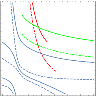
[circle, fill, scale=0.5] (x) at (-0.5, 0.5) ; [circle, fill, scale=0.5] (y) at (-0.5, 2.2) ; [right of=y] (yl) $(s,t+\delta)$ ; [right of=x] (xl) $(s,t)$ ;

[shorten ¿=10pt,shorten ¡=10pt,-¿, thick] (x) – (y);

Figure 2: Moving $\delta=\frac{1}{1-\Phi^{y}_{p}(s,t)}$ in the $y$ direction moves the point back inside the region defined by the two barrier functions.

It should now be clear how the proof proceeds — at each step, we will apply the operator $(1-\partial_{k})$ and then move our upper bound in that direction. We will bound the amount we move using the barrier function in that direction, while also taking care that we have moved far enough to cause the barrier functions in all of the other directions to go down (so that they will still be small when the time comes to use them).

Proof 0.15 (Proof of Theorem 0.1).

Let

$$P(y_{1},\dots,y_{m})=\mydet{\sum_{i=1}^{m}y_{i}A_{i}}.$$

Set $t=\sqrt{\epsilon}+\epsilon$. As all of the matrices $A_{i}$ are positive semidefinite and

$$\mydet{t\sum_{i}A_{i}}=\mydet{tI}>0,$$

the vector $t\bvec{1}$ is above the roots of $P$.

By Theorem LABEL:thm:jacobi,

$$\Phi^{i}_{P}(y_{1},\dots,y_{m})=\frac{\partial_{i}P(y_{1},\dots,y_{m})}{P(y_{1},\dots,y_{m})}=\trace{\left(\sum_{i=1}^{m}y_{i}A_{i}\right)^{-1}A_{i}}.$$

So,

$$\Phi^{i}_{P}(t\bvec{1})=\trace{A_{i}}/t\leq\epsilon/t=\epsilon/(\epsilon+\sqrt{\epsilon}),$$

which we define to be $\phi$. Set

$$\delta=1/(1-\phi)=1+\sqrt{\epsilon}.$$

For $k\in[m]$, define

$$P_{k}(y_{1},\dots,y_{m})=\left(\prod_{i=1}^{k}1-\partial_{y_{i}}\right)P(y_{1},\dots,y_{m}).$$

Note that $P_{m}=Q$.

Set $x^{0}$ to be the all-$t$ vector, and for $k\in[m]$ define $x^{k}$ to be the vector that is $t+\delta$ in the first $k$ coordinates and $t$ in the rest. By inductively applying Lemmas 0.12 and 0.14, we prove that $x^{k}$ is above the roots of $P_{k}$, and that for all $i$

$$\Phi^{i}_{P_{k}}(x^{k})\leq\phi.$$

It follows that the largest root of

$$\mixed{A_{1},\dots,A_{m}}{x}=P_{m}(x,\dots,x)$$

is at most

$$t+\delta=1+\sqrt{\epsilon}+\sqrt{\epsilon}+\epsilon=(1+\sqrt{\epsilon})^{2}.$$