Neural Network Multitask Learning for Traffic Flow Forecasting

Abstract

Traditional neural network approaches for traffic flow forecasting are usually single task learning (STL) models, which do not take advantage of the information provided by related tasks. In contrast to STL, multitask learning (MTL) has the potential to improve generalization by transferring information in training signals of extra tasks. In this paper, MTL based neural networks are used for traffic flow forecasting. For neural network MTL, a backpropagation (BP) network is constructed by incorporating traffic flows at several contiguous time instants into an output layer. Nodes in the output layer can be seen as outputs of different but closely related STL tasks. Comprehensive experiments on urban vehicular traffic flow data and comparisons with STL show that MTL in BP neural networks is a promising and effective approach for traffic flow forecasting.

I Introduction

With the rapid development of modern economy, more and more people start to use automobiles. Urban traffic congestion has become a commonplace phenomenon, which brings a series of social problems to our lives. If traffic conditions, especially the coming of peak traffic flows, can be predicted accurately, people could respond in advance to prevent roads from being jammed. Smooth and well-ordered traffic will give a great convenience to the public and our society. The establishment of a better traffic flow forecasting model is the basis of predicting traffic flows to avoid the congestion situation. For example, it could provide valuable traffic information to Intelligent Transportation Systems (ITS) to anticipate congestion occurrence as early as possible.

So far, people have raised a variety of methods for traffic flow forecasting, such as nonparametric methods [1], local regression models [2,3], neural network approaches [4], fuzzy-neural approaches [5], Markov chain models [6], and Bayesian network approaches [7]. In this paper, exploring the performance of neural networks from a new point of view for traffic flow forecasting is our concern.

A neural network (NN) is an approximation and variation to a biological neural system but is highly simplified. It has various intelligent processing functions such as learning, memorizing and predicting. NNs can solve modeling problems for complicated systems which are uncertain and seriously non-linear [8]. The traditional neural network approach for traffic flow forecasting is to learn a task at a time [9]. It is a single task learning (STL) model which neglects the potential and rich information resources hidden in other related tasks. The opposite is the multitask learning (MTL) neural network approach which has more than one output [10]. In MTL, the task considered most is called the main task, while others are called extra tasks. MTL can improve generalization performance of neural networks by integrating some field-specific training information contained in the extra tasks [11]. In this paper, we focus on using MTL backpropagation (BP) networks to carry out traffic flow modeling and forecasting. Experiments with encouraging results show that this approach is considerably effective for traffic flow modeling and forecasting.

The rest of this paper is organized as follows. MTL and its benefits for traffic flow forecasting are introduced in Section II. Then we give the model construction mechanism, and report experimental results in Section III. Section IV summarizes this paper and gives future research directions.

II MTL

II-A MTL and NN

MTL is a form of inductive transfer whose main goal is to improve generalization performance [12]. It uses the domain-specific information which is included in the training signals of extra tasks to improve generalization. In fact, the training signals for the extra tasks serve as an inductive bias [13]. In other words, that bias is used to improve the generalization accuracy in order to perfectly complete the main task. It is because that the helping information which is provided by inductive bias is stronger than the one gained without the extra knowledge. As reported, better generalization can often be yielded by employing MTL if there is only a fixed training set [14]. MTL also can be used to reduce the number of training patterns needed to achieve some fixed level of performance [15].

Normally, most learning methods such as traditional neural networks only have one task. When we want to solve a complicated problem, it could be split into a number of small, appropriately independent subproblems to learn [16]. This may ignore a potentially rich source of information contained in the training signals of other tasks drawn from the same domain [17]. In fact, it is believed that most-real-world problems are multitask problems and performances are being sacrificed when we treat them as single problems. Therefore, we introduce MTL NN which has more than one output to predict traffic flows. In a MTL NN, all tasks are trained in parallel using a shared representation. And the information contained in these extra training signals can help the hidden layer learn a better internal representation for the main task. MTL has the potential to meliorate the prediction accuracy of the main task and improve the generalization of the entire network through learning the extra tasks.

With the inductive bias provided by the extra tasks, MTL is applicable to any learning methods to improve generalization performance. Besides, the speed of learning, and the intelligibility of learned models are also ameliorated via employing MTL. This paper concentrates on improving generalization accuracy of neural networks using the inductive transfer paradigm MTL.

II-B MTL for traffic flow forecasting

MTL is broadly applicable. One of the applications is using the future to predict the present [18]. Time series prediction is the subclass of using the future to predict the present. MTL used for series prediction is a new method for traffic flow forecasting whose core idea is to make prediction for the same task at different time. Using MTL NN to make time series prediction, the simplest approach is to use a network with a number of outputs, each output corresponding to one task which is at different time. In addition, the output used for prediction can be the middle one so that there are tasks earlier and later than it trained in the net [11].

The flow of one traffic junction at any time has a correlation with the flow of its contiguous moment. Therefore, using time series prediction to forecast traffic flow has significance. We can arbitrarily choose the flow of m continuous time instants to forecast their next moment’s flow. The way we use MTL is that we predict the vehicle flow at time n (denoted by t(n)) by selecting t(n-1) and t(n+1) as well as outputs. Therefore, forecasting t(n) is treated as the main task in the network. We generally select the extra tasks which definitely have connections with the main tasks. Here, we consider that t(n-1) and t(n+1) have certain relationship with the main task and choose them as extra tasks. They play an inductive bias role for the main task so as to increase the forecasting accuracy of t(n).

III Model construction and experiments

III-A The source of data

Now, we use the idea of time series prediction for traffic flow forecasting, and the net is BP neural network using MTL. It means that we forecast future traffic flow at given road links from the historical data of themselves. The difference from ordinary neural network is that the current uses a method of MTL. It has more than one output.

The data used for analysis are the vehicle flow rates of discrete time series which were recorded every 15 min. Data’s unit is vehicles per hour (veh/h). We choose a fraction taken from one urban traffic map of highways to verify the approach of MTL. The fraction is shown in Fig. 1. Each circle node in the sketch map denotes a road junction. An arrow shows the direction of traffic flow, which reaches the corresponding road link from its upstream link. Paths without arrows are of no traffic flow records. The raw data are from March 1 to March 31, 2002, totaling 31 days [7]. Considering the malfunction of detector or transmitter, we screened the days with empty data in view of evaluation. The remaining data for use are of 25 days and totaling 2400 sample points. We select the first 2112 samples points and treat them as training data. The rest are used for test data.

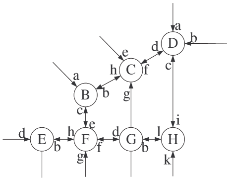
Figure 1: Patch taken from the East Section of the Third Circle of Beijing City Map where UTC/SCOOT systems are placed. For convenience, roads and flows are coded with English characters.

III-B Model building

The model building of the traffic flow forecasting can be concluded as follows:

(1). A three-layer NN is chosen. The reason is that it can approximate to any continuous function, as long as the appropriate number of hidden layer neurons and right activation functions are used. If the network layers increase, the network will become complicated and the training time will increase. Therefore, a network which has an input layer, a hidden layer and an output layer is selected.

(2). Traffic flows of five seriate time instants are adopted as inputs. A function which can make data normalize to deal with the sample points is applied. After doing that, the original data are normalized to the range -1 from 1. At the same time, the pace of training may accelerate. After normalization, the initial weights of network will not be big, enabling network performance and the ability of generalization better. For the hidden layer we select fifteen neurons according to practical training performance.

(3). Sigmoid function is selected as the specific activation function between input layer and hidden layer. The form of sigmoid function is described as

$$\ f(x)=\frac{2}{1+e^{-2x}}-1.$$ (1)

This function can make neuronal inputs map to a range from -1 to 1 . Since it is a differentiable function which is suitable to train NN using the algorithm of BP. The activation function between hidden layer and output layer is a linear function whose form is shown as

$$\ f(x)=x.$$ (2)

It is also a differentiable function. We can get arbitrary value from the function as its outputs.

(4). Levenberg-Marquardt algorithm is selected to train the network [19,20]. Because it has comparatively fast convergence speed and high precision which can rectify network’s weights and threshold better. The adjustment formula is shown as

$$\ x_{k+1}=x_{k}-[J^{T}J+\mu{I}]^{-1}J^{T}e,$$ (3)

where J is a Jacobian matrix whose elements are the network error’s first derivatives with respect to weights and the corresponding threshold, e is the network error vector, and $\mu$ is a scalar quantity which is initialized.

There are many parameters in the training function including the largest training epoch, training time, and network error target which can be all acted as the stopping conditions of training. If training time of the network has no strict demands, the largest training epochs which can make the network converge are selected as the only guideline of the training stopping by observing the changes in network training error. Since the establishment of the preferable network model is based on the results of a large number of practical trainings, so only when we change a parameter to inspect the effect which is brought to the network, can we build a better network model [21].

(5). The constructed MTL network model is given in Fig. 2. The network has three outputs and the forecasting of t(n) is severed as main task. We employed STL as a comparative method and the STL network model is given in Fig. 3. As is shown, the net only has one task.The difference between that two NNs is only in their output layer. STL NN has one neuron as its output, while MTL NN not only has main task, but also has extra task.

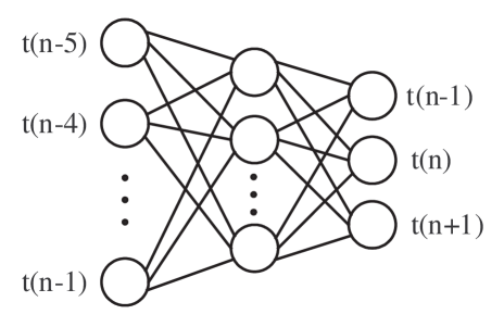
Figure 2: NN using MTL to forecast t(n).

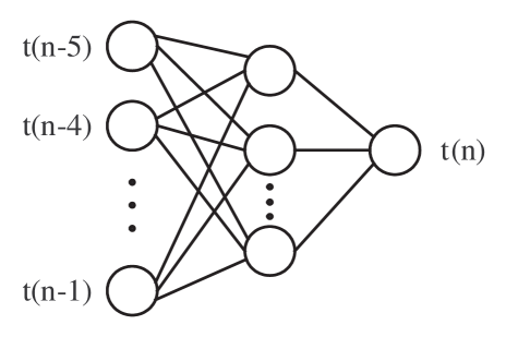
Figure 3: NN using STL to forecast t(n).

III-C Experimental results

We take vehicle flow data $\mathbf{B_{b}}$ as an instance to show our modeling mechanism. $\mathbf{B_{b}}$ represents the vehicle flow from upstream junction C to downstream junction B. The traffic flow figure of all sample points in 25 days is depicted in Fig. 4.

The training set and test set have been described, we predict traffic flow only for single inflow of a junction. The network is trained by using the first 22 days’ data to forecast the traffic flow of later 3 days. Experiments are firstly done by using MTL. According to practical training, setting training parameters of the NN. The goal of training error is initially defined as 0.006. In course of the experiment, training error of the network is shown in Fig. 5.

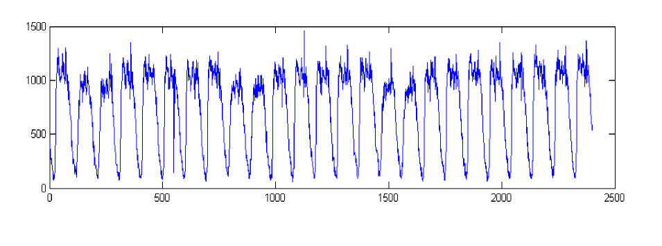
Figure 4: The original value of traffic flow $\mathbf{B_{b}}$.

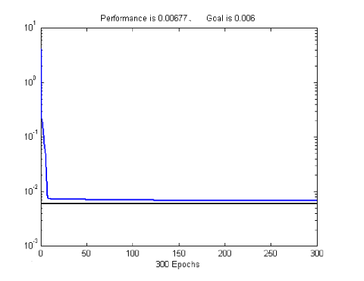
Figure 5: Network training error of $\mathbf{B_{b}}$. The curve represents the changed condition of error in the course of training, the horizontal line denotes the goal of training error.

From Fig. 5, we can see that network error hardly changes after 125 training steps. In order to increase the training accuracy, 300 epochs are selected as the maximal training epochs in the end. It also means that the training will stop after experiencing 300 training epochs.

The final forecasting result of the MTL network for the last 3 days’ data of link $\mathbf{B_{b}}$ is shown in Fig. 6.

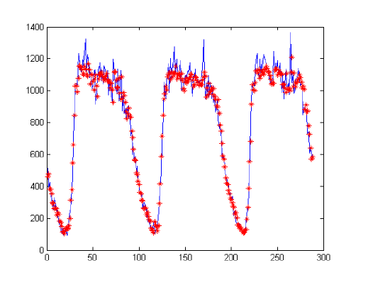
Figure 6: MTL traffic flow forecasting result for the last 3 days’ data of road link $\mathbf{B_{b}}$.

Root mean square error (RMSE) is used to evaluate prediction performance of the networks. The expression is shown as

$$\ RMSE=({\sum_{i=0}^{n}}{\frac{(t(i)-\alpha(i))^{2}}{n}})^{1/2},$$ (4)

where $\alpha$ is the estimate of n-dimensional vector t. The performance measure RMSE of $\mathbf{B_{b}}$ in MTL can be calculated as the following:

$$\ RMSE_{M}=70.25.$$ (5)

Now, we employed STL as a comparative method. The final forecasting result of the STL network for the last 3 days’ data of link $\mathbf{B_{b}}$ is shown in Fig. 7. Similarly the RMSE is:

$$\ RMSE_{S}=77.46.$$ (6)

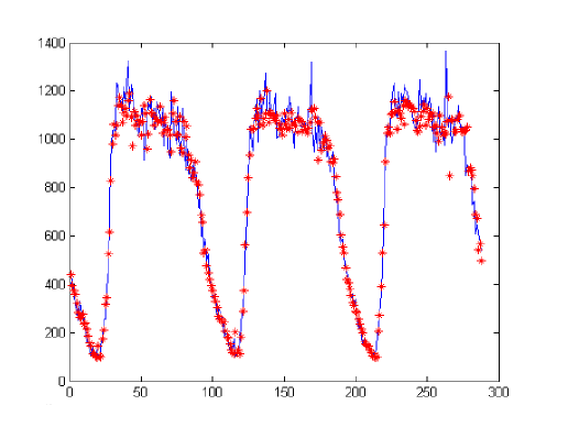
Figure 7: STL traffic flow forecasting result for the last 3 days’ data of road link $\mathbf{B_{b}}$.

Known from formula (5) and formula (6), MTL is better than STL in forecast accuracy. Furthermore, the performance improvement of MTL is defined as follows:

$$\ {{e}_{B}}_{b}=\frac{{RMSE}_{S}-{RMSE}_{M}}{{RMSE}_{S}}=9.31\%$$ (7)

This is meant that MTL is better than STL in prediction accuracy by 9.31 percent. In order to objectively evaluate the performance of STL and MTL for traffic flow forecasting, we also conduct experiments on other road links. Likewise, we select the largest training epochs which can make the network converge as the only guideline of the training stopping. The other parameters are all based on the results of a large number of practical trainings. The results are given in Table I.

TABLE I: Comparison results with STL

​RMSE​	$\mathbf{C_{f}}$	$\mathbf{D_{b}}$	$\mathbf{F_{f}}$	$\mathbf{G_{b}}$	$\mathbf{H_{i}}$	$\mathbf{B_{b}}$
STL	$93.03$	$55.04$	$85.28$	$84.89$	$92.28$	$77.46$
MTL	$86.26$	$52.85$	$82.02$	$82.90$	$88.02$	$70.25$
e	$7.28$%	$3.98$%	$3.82$%	$2.34$%	$4.62$%	$9.31$%

From the results, we can see that RMSE of the forecasting results all diminish after using MTL. It implies that the forecasting precision is improved. Therefore, MTL NN can be used for traffic flow forecasting to get relatively precise results. It is useful for ITS to deal with the problem of traffic congestion.

IV Conclusion

Traditional forecasting methods are generally to anticipate with STL. They fail to attach importance to a potential, rich and available information resources which can be obtained from training information of other tasks in the same area. Usually, those results are not ideal. MTL mentioned in this paper is synchronal to train more than one task and can take full advantage of training information in the extra tasks to improve the generalization of the network. It makes the net have higher forecasting accuracy.

From above experiments, we can see that the forecasted results of traffic flows are closer to the true value when multitask learning is used in the network. It illuminates that multi-task learning for time series prediction of traffic flow is very practical. In the future, comparing the neural network MTL approach with other methods, such as kernel regression [1,11], Bayesian networks [7] will be investigated. Besides, incorporating information from neighbor road links would also be studied [22].

References

- [1] G. A. Davis and N. L. Nihan, “Non-parametric regression and short-term freeway traffic forecasting,” J. Transp. Eng., vol. 177, no. 2, pp. 178 C188, 1991.
- [2] G. A. Davis, “Adaptive forecasting of freeway traffic congestion,” Transp. Res. Rec., no. 1287, pp. 29-33, 1990.
- [3] B. L. Smith and M. Demetsky, “Traffic flow forecasting: Comparison of modeling approaches,” J. Transp. Eng., vol. 123, no. 4, pp. 261-266, 1997.
- [4] J. Hall and P.Mars, “The limitations of artificial neural networks for traffic prediction,” in Proc. 3rd IEEE Symp. Computers and Communications, Athens, Greece, pp. 8-12, 1998.
- [5] H. B. Yin, S. C. Wong, J. M. Xu, and C. K. Wong, “Urban traffic flow prediction using a fuzzy-neural approach,” Transp. Res., Part C Emerg. Technol., vol. 10, no. 2, pp. 85-98, Apr. 2002.
- [6] G. Q. Yu, J. M. Hu, C. S. Zhang, L. K. Zhuang, and J. Y. Song, “Shortterm traffic flow forecasting based on Markov chain model,” in Proc. IEEE Intelligent Vehicles Symp., Columbus, OH, pp. 208-212, 2003.
- [7] S. Sun, C. Zhang, and G. Yu, “A Bayesian network approach to traffic flow forecasting,” IEEE Transactions on Intelligent Transportation Systems, vol. 7, no. 1, march 2006.
- [8] C. Rich and R. S. Virginia , “Benefiting from the variables that variable selection discards,” Journal of Machine Learning Research, 3, pp. 1245-1264, 2003.
- [9] B. M. William, “Modeling and forecasting vehicular traffic flow as a seasonal stochastic time series process,” Ph. D. Dissertation, Dept. Civil Eng., Univ. Virginia, Charlottesville, VA, 1999.
- [10] S. Thrun, and T. Mitchell, “Learning one more thing,” Carnegie Mellon University: CS-94-184, 1994.
- [11] C. Rich , “Multitask learning,” Machine Learning, 28(1), 41-75(1997).
- [12] J. Ghosn and Y. Bengio, “Multi-task learning for stock selection,” Neural Information Processing Systems 9, (Proceedings of NIPS-96), 1997.
- [13] J. Baxter, “A model for inductive bias learning,” Journal of Artificial Intelligence Research, 12, pp. 149-198, 2000.
- [14] V. Tresp, S. Ahmad, and R. Neuneier, “Training neural networks with deficient data,” Neural Information Processing Systems 6, (Proceedings of NIPS-93), pp. 128-135, 1994.
- [15] S. Ben-David and R. Schuller, “Exploiting task relatedness for multiple task learning,” Proceedings of Computational Learning Theory (COLT), 2003.
- [16] R. Caruana, “Multitask learning: A knowledge-based source of inductive bias,” Proceedings of the 10th International Conference on Machine Learning, ML-93, University of Massachusetts, Amherst, pp. 41-48, 1993.
- [17] R. Caruana, “Learning many related tasks at the same time with backpropagation,” Advances in Neural Information Processing Systems 7, (Proceedings of NIPS-94), pp. 656-664, 1995.
- [18] M. Der Voort, M. Dougherty, and S. Watson, “Combining kohonen maps with ARIMA time series models to forecast traffic flow,” Transp. Res., Part C Emerg. Technol., vol. 4, no. 5, pp. 307-318, Oct. 1996.
- [19] S. Xi, Nonlinear Optimization Methods, Higher Education Press, 1992.
- [20] Y. Yuan, and W. Sun, The Optimization Theory and Methods, Science Press, 1997.
- [21] H. Demuth and M. Beale, Neural Network Toolbox User’s Guide for Use with MATLAB,(4thEd.), the Mathworks Inc., 2001.
- [22] S. Sun, C. Zhang, and Y. Zhang, “Traffic flow forecasting using a spatio-temporal prediction,” ICANN(2), pp. 273-278, 2005.