Let’s Make Block Coordinate Descent Converge Faster:
Faster Greedy Rules, Message-Passing,
Active-Set Complexity, and Superlinear Convergence

Abstract

Block coordinate descent (BCD) methods are widely used for large-scale numerical optimization because of their cheap iteration costs, low memory requirements, amenability to parallelization, and ability to exploit problem structure. Three main algorithmic choices influence the performance of BCD methods: the block partitioning strategy, the block selection rule, and the block update rule. In this paper we explore all three of these building blocks and propose variations for each that can significantly improve the progress made by each BCD iteration. We (i) propose new greedy block-selection strategies that guarantee more progress per iteration than the Gauss-Southwell rule; (ii) explore practical issues like how to implement the new rules when using “variable” blocks; (iii) explore the use of message-passing to compute matrix or Newton updates efficiently on huge blocks for problems with sparse dependencies between variables; and (iv) consider optimal active manifold identification, which leads to bounds on the “active-set complexity” of BCD methods and leads to superlinear convergence for certain problems with sparse solutions (and in some cases finite termination at an optimal solution). We support all of our findings with numerical results for the classic machine learning problems of least squares, logistic regression, multi-class logistic regression, label propagation, and L1-regularization.

Keywords: Convex optimization, convergence rates, block coordinate descent, greedy algorithms, large-scale

1 Introduction

Block coordinate descent (BCD) methods have become one of the key tools for solving some of the most important large-scale optimization problems. This is due to their typical ease of implementation, low memory requirements, cheap iteration costs, adaptability to distributed settings, ability to use problem structure, and numerical performance. Notably, they have been used for almost two decades in the context of L1-regularized least squares (LASSO) (Fu, 1998; Sardy et al., 2000) and support vector machines (SVMs) (Chang and Lin, 2011; Joachims, 1999). Indeed, randomized BCD methods have recently been used to solve instances of these widely-used models with a billion variables (Richtárik and Takáč, 2014), while for “kernelized” SVMs greedy BCD methods remain among the state of the art methods (You et al., 2016). Due to the wide use of these models, any improvements on the convergence of BCD methods will affect a myriad of applications.

In recent work, we have given a refined analysis of greedy coordinate descent in the special case where we are updating a single variable (Nutini et al., 2015). This work supports the use of greedy coordinate descent methods over randomized methods in the many scenarios where the iterations costs of these methods are similar. Other authors have subsequently shown a variety of interesting results related to greedy coordinate descent algorithms (Locatello et al., 2018; Song et al., 2017; Stich et al., 2017; Lu et al., 2018; Karimireddy et al., 2019; Fang et al., 2020). These works also focus on the case of updating a single coordinate, and do not explore the large design space of possible choices we could make when updating multiple coordinates in a block. An exception to this is Csiba and Richtárik (2017), which was contemporaneous with the first version of this work and whose “greedy minibatch” strategy is obtained as special case of a greedy BCD rule we present in Section 3.

The work described in this paper is motivated by the plethora of choices available when implementing greedy BCD. In this work we survey a variety of choices that are available in the literature, present new choices for several problem structures, and present both theoretical and empirical evidence that some choices are superior to others. By considering the conclusions from this paper and a particular problem structure that a reader is interested in, we expect that readers should be able to develop substantially-faster BCD algorithms for many applications. Further, some of the lessons we learned from this work can also be used to give faster algorithms in other settings like cyclic and randomized BCD.

While there are a variety of ways to implement a BCD method, the three main building blocks that affect its performance are:

1. Blocking strategy. We need to define a set of possible “blocks” of problem variables that we might choose to update at a particular iteration. Two common strategies are to form a partition of the coordinates into disjoint sets (we call this fixed blocks) or to consider any possible subset of coordinates as a “block” (we call this variable blocks). Typical choices include using a set of fixed blocks related to the problem structure, or using variable blocks by randomly sampling a fixed number of coordinates.

2. Block selection rule. Given a set of possible blocks, we need a rule to select a block of corresponding variables to update. Classic choices include cyclically going through a fixed ordering of blocks, choosing random blocks, choosing the block with the largest gradient (the Gauss-Southwell rule), or choosing the block that leads to the largest improvement.

3. Block update rule. Given the block we have selected, we need to decide how to update the block of corresponding variables. Typical choices include performing a gradient descent iteration, computing the Newton direction and performing a line-search, or computing the optimal update of the block by subspace minimization.

In Section 2 we introduce our notation, review the standard choices behind BCD algorithms, and discuss problem structures where BCD is suitable. Subsequently, the following sections explore a wide variety of ways to speed up BCD by modifying the three building blocks above. In particular, we first consider the implementation issues associated with using greedy BCD methods for general unconstrained optimization:

• In Section 3 we propose selection rules that generalize the Gauss-Southwell-Lipschitz rule proposed in Nutini et al. (2015). The Gauss-Southwell-Lipschitz rule incorporates knowledge of Lipschitz constants into the classic Gauss-Southwell rule in order to give a better bound on the progress made at each iteration. The prior work considered this rule in the setting of updating a single coordinate, and in this work we propose several generalizations to the block setting. We also show a result characterizing the convergence rate obtained using the Gauss-Southwell rule as well as the new greedy rules, under both the Polyak-Łojasiewicz inequality and for general (potentially non-convex) functions.

• In Section 4 we discuss a variety of the practical implementation issues associated with implementing BCD methods. This includes how to approximate the new rules in the variable-block setting, how to estimate the Lipschitz constants, how to efficiently implement line-searches, how the blocking strategy interacts with greedy rules, and why we should prefer Newton updates over the “matrix updates” of recent works. While we specifically discuss these in the context of greedy methods, several of the ideas in this section also apply when implementing cyclic or randomized BCD methods.

In the next sections we consider two of the most-common cases where BCD methods are used. In particular, we consider problems with a sparse dependency structure and problems that include a non-smooth but separable term. In this context we make the following contributions:

• In Section 5 we show how second-order updates, or the exact update for quadratic functions, can be computed in linear-time for problems with sparse dependencies when using “forest-structured” blocks. This allows us to use huge block sizes for problems with sparse dependencies, and uses a connection between sparse quadratic functions and Gaussian Markov random fields (GMRFs) by exploiting the “message-passing” algorithms developed for GMRFs. We discuss how to efficiently construct forest-structured blocks in both randomzied and greedy settings.

• In Section 6 we give bounds on the number of iterations required to reach the optimal manifold (“active-set complexity”) when applying greedy (or cyclic) BCD methods to problems with a separable non-smooth structure. We also discuss how when using greedy rules with variable blocks this leads to local superlinear convergence for problems with sufficiently-sparse solutions (when we use updates incorporating second-order information). This leads to finite convergence for problems with sufficiently-sparse solutions and where exact updates are possible (such as SVMs and LASSO problems), when using greedy selection and sufficiently-large variable blocks. We further discuss how the old idea of two-metric projection can be used to obtain this finite convergence while maintaining the cost of BCD methods for smooth objectives.

We note that many related ideas have been explored by others in the context of BCD methods and we will go into detail about these related works in the relevant sections. In Section 7 we use a variety of problems arising in machine learning to evaluate the effects of these choices on BCD implementations. These experiments indicate that in some cases the performance improvement obtained by using these enhanced methods can be dramatic.

Below we list 7 hypotheses that our work supports regarding the implementation of BCD methods, along with the relevant theoretical and/or empirical results in this work. When implementing BCD methods, we recommend to consider each of these issues and to follow the guideline provided that it does not substantially increase the iteration cost.

1. Similar to the the case of updating a single coordinate, BCD methods tend to converge faster when using greedy rules than random or cyclic rules. Thus, we should prefer greedy methods in cases where their iteration costs are similar to those of cyclic/random methods. We discuss these classic block selection rules in Section 2.1 and we discuss problem structures where random and greedy methods can be efficiently implemented in Sections 2.4-2.5 (with a detailed example in Appendix A). We give a bound showing why greedy methods may converge faster in Section 3.1, while empirical evidence for the advantage of greedy methods is seen in Sections 7.1, 7.3-7.4, and Appendix F.2.

2. All BCD methods tend to converge faster as the block size increases. Thus, it is beneficial to use larger blocks in cases where this does not increase the iteration cost. The main reasons why it might not increase the cost are the use of parallel computation, or the presence of special problem structures that make updating particular blocks of variables have the same cost as updating a single variable (we give an example in Appendix A). Section 3.1 gives a bound showing why increasing the block size tends to improves the progress per iteration, while empirical evidence for faster convergence as we increase the block size is seen in Sections 7.1-7.3, Appendix F.2, and Appendix F.3.

3. When using greedy selection rules, using variable blocks can substantially outperform using fixed blocks. When using randomized rules, we observed the opposite trend: we found that using fixed blocks tended to outperform variable blocks within randomized BCD methods. We discuss fixed and variable blocks in Section 2.2. Section 3.1 discusses why variable blocks lead to a better progress bound on each iteration for greedy methods, and this is empirically supported by the experiments in Sections 7.1- 7.2, Appendix F.2, an Appendix F.3

4. We found that using the new block versions of the Gauss-Southwell-Lipschitz rules can lead to substantially-faster convergence than the classic Gauss-Southwell rule. This gain was much larger than the modest improvements seen from the Gauss-Southwell-Lipschitz in prior work that only considered the single-coordinate case. On the other hand, we did not observe large differences between the various block generalizations of the Gauss-Southwell-Lipschitz rule, indicating that we can use the computationally-cheaper variants of the rule. These new Gauss-Southwell-Lipschitz rules are introduced in Sections 3.2-3.4, which discuss why these rules tend to make more progress per iteration than the classic GS rule. Formal convergence rates are given in Sections 3.5-3.6. We discuss how to efficiently implementing this type of rule in Section 4.1 (while Appendix B discusses how to compute Lipschitz constants for some common problems). Empirical support for the advantages of the new rules is seen in Sections 7.1-7.2, Appendix F.2, and Appendix F.3.

5. We found that updates that scale the gradient by a matrix tend to outperform updates that use the gradient direction. Further, applying Newton’s method to the block tended to outperform the fixed matrix scalings used in several recent works. We discuss matrix updates and Newton’s method in Section 2.3. Section 3.3 shows why matrix updates tend to make more progress per iteration, with convergence rates given in Sections 3.5-3.6. The difference between using gradient updates and matrix updates can be observed by comparing the experiments in Section 7.1 to the experiments in Section 7.2, and by comparing the experiments in Appendix F.2 to the experiments in Appendix F.3. Section 4.6 discusses why Newton updates should give a further improvement over matrix updates, and empirical evidence for the advantage of Newton updates is given in Appendix F.3.

6. For problems with sparse dependencies, we found that using large forest-structured blocks can give a substantial peformance improvement over unstructured blocks (which must be much smaller to have a comparable cost). This applied whether we used random or greedy methods to construct the forest-structured blocks. Sections 5.1-5.3 discuss how to implement forest-structured updates in linear time, Sections 5.4-5.6 and Appendix D discuss how to efficiently construct forest-structured blocks, and Section 7.3 shows experimentally that forest-structured blocks can lead to a huge performance gain.

7. For non-smooth problems with sparse solutions, the performance difference between random and greedy methods can be even larger than for smooth problems. This is because the greedy methods tend to focus on updating non-zero variables. Sections 6.1-6.2 show the speed at which greedy methods identify the set of non-zero variables, while Sections 6.3-6.5 discuss rules and updates that lead to superlinear convergence for certain non-smooth problems when using greedy rules with variable blocks. Section 7.4 shows experimentally the performance gains obtained by using variable blocks and rules/updates that give superlinar convergence, while Appendix F.4 shows the relative innefficiency of using randomized updates for this problem setting. Further, for obtaining superlinear convergence on non-smooth problems, the efficient two-metric projection strategies for updating the blocks has nearly the same convergence rate as the more-expensive projected-Newton updates. The two-metric projection method is discussed in Section 6.4, while Section 7.4 shows that the method has essentially-identical performance in practice to using more-expensive rules.

We also found that using a line-search or local approximations of the Lipschitz constants led to faster convergence than using global upper bounds on these constants. This was particularly noticeable as we increased the block size. We discuss how to use local approximations of the Lipschitz constants in Section 4.3, and how to efficiently implement line-searches for notable problem structures in Section 4.4. This is supported empirically in Appendix F.2 andAppendix F.3. However, when using approximations to Lipschitz constants we need to be careful about how it affects selection rules that depend on the Lipschitz constants (we observe a case where using approximated Lipshitz information within the selection hurts performance in Appendix F.2).

We summarize a set of recommendations that our experiments support in the table below:

Premise	Recommendation
Random BCD has similar cost to gradient descent.	Do not use BCD.
Greedy BCD has similar cost random BCD.	Use greedy selection.
BCD with large blocks has similar cost to small blocks.	Use bigger blocks.
Using random BCD.	Use fixed blocks.
Using greedy BCD, variable blocks have similar cost to fixed blocks.	Use variable blocks.
Using greedy BCD, any GSL rule has similar cost to GS rule.	Use GSL.
Using greedy BCD wth fixed blocks, and have Lipschitz constants.	Partition blocks using sort strategy.
Matrix updates have similar cost to gradient updates.	Do not use gradient updates.
Newton updates have similar cost to matrix updates.	Use Newton updates.
Using matrix/Newton updates and dependencies are very sparse.	Use forest-structured blocks.
Using matrix/Newton updates but have non-differentiable regularizer.	Use two-metric projection.
Function is not quadratic.	Set the step-size with a line-search.

The source code and data files required to reproduce the experimental results of this paper can be downloaded from: https://github.com/IssamLaradji/BlockCoordinateDescent.

2 Block Coordinate Descent Algorithms

We first consider the problem of minimizing a differentiable multivariate function,

$$\mathop{\hbox{arg\,min}}_{x\in{\rm I\!R}^{n}}f(x).$$ (1)

At iteration $k$ of a BCD algorithm, we first select a block $b_{k}\subseteq\{1,2,\dots,n\}$ and then update the subvector $x_{b_{k}}\in{\rm I\!R}^{|b_{k}|}$ corresponding to these variables,

$$x^{k+1}_{b_{k}}=x^{k}_{b_{k}}+d^{k}.$$

Coordinates of $x^{k+1}$ that are not included in $b_{k}$ are simply kept at their previous value. The vector $d^{k}\in{\rm I\!R}^{|b_{k}|}$ is typically selected as a descent direction in the reduced dimensional subproblem,

$$d^{k}\in\mathop{\hbox{arg\,min}}_{d\in{\rm I\!R}^{|b_{k}|}}f(x^{k}+U_{b_{k}}d),$$ (2)

where we construct $U_{b_{k}}\in\{0,1\}^{n\times|b_{k}|}$ from the columns of the identity matrix corresponding to the coordinates in $b_{k}$. Using this notation, we have

$$x_{b_{k}}=U_{b_{k}}^{T}x,$$

which allows us to write the BCD update of all $n$ variables in the form

$$x^{k+1}=x^{k}+U_{b_{k}}d^{k}.$$

There are many possible ways to define the block $b_{k}$ as well as the direction $d^{k}$. Typically we have a maximum block size $\tau$, which is chosen to be the largest number of variables that we can efficiently update at once. Given $\tau$ that divides evenly into $n$, consider a simple ordered fixed partition of the coordinates into a set $\mathcal{B}$ of $n/\tau$ blocks,

$$\mathcal{B}=\{\{1,2,\dots,\tau\},\{\tau+1,\tau+2,\dots,2\tau\},\dots,\{(n-\tau)+1,(n-\tau)+2,\dots,n\}\}.$$

To select the block in $\mathcal{B}$ to update at each iteration we could simply repeatedly cycle through this set in order. A simple choice of $d^{k}$ is the negative gradient corresponding to the coordinates in $b_{k}$, multiplied by a scalar step-size $\alpha_{k}$ that is sufficiently small to ensure that we decrease the objective function. This leads to a gradient update of the form

$$x^{k+1}=x^{k}-\alpha_{k}U_{b_{k}}\nabla_{b_{k}}f(x^{k}),$$ (3)

where $\nabla_{b_{k}}f(x^{k})$ are the elements of the gradient $\nabla f(x^{k})$ corresponding to the coordinates in $b_{k}$. While this gradient update and cyclic selection among an ordered fixed partition is simple, we can often drastically improve the performance using more clever choices. We highlight some common alternative choices in the next three subsections.

2.1 Block Selection Rules

Repeatedly going through a fixed partition of the coordinates is known as cyclic selection (Bertsekas, 2016), and this is referred to as Gauss-Seidel when solving linear systems (Ortega and Rheinboldt, 1970). The performance of cyclic selection may suffer if the order the blocks are cycled through is chosen poorly, but it has been shown that random permutations can fix a worst case for cyclic CD (Lee and Wright, 2019). A variation on cyclic selection is “essentially” cyclic selection where each block must be selected at least every $m$ iterations for some fixed $m$ that is larger than the number of blocks (Bertsekas, 2016). Alternately, several authors have explored randomized block selection (Nesterov, 2012; Richtárik and Takáč, 2014). The simplest randomized selection rule is to select one of the blocks uniformly at random. However, several recent works show dramatic performance improvements over this naive random sampling by incorporating knowledge of the Lipschitz continuity properties of the gradients of the blocks (Nesterov, 2012; Richtárik and Takáč, 2016; Qu and Richtárik, 2016) or more recently by trying to estimate the optimal sampling distribution online (Namkoong et al., 2017).

An alternative to cyclic and random block selection is greedy selection. Greedy methods solve an optimization problem to select the “best” block at each iteration. A classic example of greedy selection is the block Gauss-Southwell (GS) rule, which chooses the block whose gradient has the largest Euclidean norm,

$$b_{k}\in\mathop{\hbox{arg\,max}}_{b\in\mathcal{B}}\|\nabla_{b}f(x^{k})\|,$$ (4)

where we use $\mathcal{B}$ as the set of possible blocks. This rule tends to make more progress per iteration in theory and practice than randomized selection (Dhillon et al., 2011; Nutini et al., 2015). Unfortunately, for many problems it is more expensive than cyclic or randomized selection. However, several recent works show that certain problem structures allow efficient calculation of GS-style rules (Meshi et al., 2012; Nutini et al., 2015; Fountoulakis et al., 2016; Lei et al., 2016), allow efficient approximation of GS-style rules (Dhillon et al., 2011; Thoppe et al., 2014; Stich et al., 2017), or allow other rules that try to improve on the progress made at each iteration (Glasmachers and Dogan, 2013; Csiba et al., 2015; Perekrestenko et al., 2017).

The ideal selection rule is the maximum improvement (MI) rule, which chooses the block that decreases the function value by the largest amount. Notable recent applications of this rule include leading eigenvector computation (Li et al., 2015), polynomial optimization (Chen et al., 2012), and fitting Gaussian processes (Bo and Sminchisescu, 2008). While recent works explore computing or approximating the MI rule for quadratic functions (Bo and Sminchisescu, 2008; Thoppe et al., 2014), in general the MI rule is much more expensive than the GS rule.

2.2 Fixed vs. Variable Blocks

While the choice of the block to update has a significant effect on performance, how we define the set of possible blocks also has a major impact. Although other variations are possible, we highlight below the two most common blocking strategies:

1. Fixed blocks. This method uses a partition of the coordinates into disjoint blocks, as in our simple example above. This partition is typically chosen prior to the first iteration of the BCD algorithm, and this set of blocks is then held fixed for all iterations of the algorithm. We often use blocks of roughly equal size, so if we use blocks of size $\tau$ this method might partition the $n$ coordinates into $n/\tau$ blocks. Generic ways to partition the coordinates include “in order” as we did above (Bertsekas, 2016), or using a random partition (Nesterov, 2012). Alternatively, the partition may exploit some inherent substructure of the objective function such as block separability (Meier et al., 2008), the ability to efficiently solve the corresponding sub-problem (2) with respect to the blocks (Sardy et al., 2000), or based on the Lipschitz constants of the resulting blocks (Thoppe et al., 2014; Csiba and Richtárik, 2018).

2. Variable blocks. Instead of restricting our blocks to a pre-defined partition of the coordinates, we could instead consider choosing any of the $2^{n}-1$ possible sets of coordinates as our block. In the randomized setting, this is referred to as “arbitrary” sampling (Richtárik and Takáč, 2016; Qu and Richtárik, 2016). We say that such strategies use variable blocks because we are not choosing from a partition of the coordinates that is fixed across the iterations. Due to computational considerations, when using variable blocks we typically want to impose a restriction on the size of the blocks. For example, we could construct a block of size $\tau$ by randomly sampling $\tau$ coordinates without replacement, which is known as $\tau$-nice sampling (Qu and Richtárik, 2016; Richtárik and Takáč, 2016). Alternately, we could include each coordinate in the block $b_{k}$ with some probability like $\tau/n$ (so the block size may change across iterations, but we control its expected size). A version of the greedy Gauss-Southwell rule (4) with variable blocks would select the $\tau$ coordinates corresponding to the elements of the gradient with largest magnitudes (Tseng and Yun, 2009a). This can be viewed as a greedy variant of $\tau$-nice sampling. While we can find these $\tau$ coordinates for the Gauss-Southwell rule easily given the gradient vector, computing the MI rule with variable blocks is much more difficult. Indeed, while methods exist to compute the MI rule for quadratics with fixed blocks (Thoppe et al., 2014), with variable blocks it is NP-hard to compute the MI rule and existing works resort to approximations (Bo and Sminchisescu, 2008).

2.3 Block Update Rules

The selection of the update vector $d^{k}$ can significantly affect performance of the BCD method. For example, in the gradient update (3) the method can be sensitive to the choice of the step-size $\alpha_{k}$. Classic ways to set $\alpha_{k}$ include using a fixed step-size (with each block possibly having its own fixed step-size), using an approximate line-search, or using the optimal step-size (which has a closed-form solution for quadratic objectives) (Bertsekas, 2016).

A generalization of the gradient update, where $d^{k}=-\alpha_{k}\nabla_{b_{k}}f(x^{k})$, is what we will call a matrix update where

$$d^{k}=-\alpha_{k}\left(H_{b_{k}}\right)^{-1}\nabla_{b_{k}}f(x^{k}).$$ (5)

Here, $H_{b_{k}}$ can be any positive-definite matrix. A notable special case is the Newton update,

$$d^{k}=-\alpha_{k}\left(\nabla^{2}_{b_{k}b_{k}}f(x^{k})\right)^{-1}\nabla_{b_{k}}f(x^{k}),$$ (6)

where $H_{b_{k}}$ is chosen as the instantaneous Hessian of the block $\nabla^{2}_{b_{k}b_{k}}f(x^{k})$ (or a positive-definite approximation to this quantity). In this context $\alpha_{k}$ is again a step-size that can be chosen using similar strategies to those mentioned above. Several recent works analyze various forms of matrix updates and show that they can substantially improve the convergence rate (Tappenden et al., 2016; Qu et al., 2016; Fountoulakis and Tappenden, 2018; Rodomanov and Kropotov, 2020; Mutny et al., 2020). For special problem classes, another possible type of update is what we will call the optimal update. This update chooses $d^{k}$ to solve (2). In other words, it updates the block $b_{k}$ to maximally decrease the objective function.

2.4 Problems of Interest

BCD methods are not suitable for all problems, since for some problems computing the gradient with respect to a block of variables has the same cost as computing the full gradient vector. It is thus important to consider the sets of problem for which they are appropriate. BCD methods tend to be suitable when the cost of updating a block of size $|b_{k}|$ is $\tilde{O}((|b_{k}|/n)\kappa)$, where $\kappa$ is the cost of computing the full gradient. Two common classes of objective functions where single-coordinate descent methods $(|b_{k}|=1)$ tend to be suitable are

$$h_{1}(x):=\sum_{i=1}^{n}g_{i}(x_{i})+f(Ax),\quad\text{or}\quad h_{2}(x):=\sum_{i\in V}g_{i}(x_{i})+\sum_{(i,j)\in E}f_{ij}(x_{i},x_{j}),$$

where $f$ is smooth and cheap, the $f_{ij}$ are smooth, $G=\{V,E\}$ is a graph, and $A$ is a matrix. Examples of problems leading to functions of the form $h_{1}$ include least squares, logistic regression, LASSO, and SVMs. The most important example of problem $h_{2}$ is quadratic functions, which are crucial to many aspects of scientific computing.

Problems $h_{1}$ and $h_{2}$ are also suitable for BCD methods, as they tend to admit efficient block update strategies. In general, if single-coordinate descent is efficient for a problem, then BCD methods with gradient updates (3) are also efficient for that problem and this applies whether we use fixed blocks or variable blocks. In Nutini et al. (2015, Appendix A) we discuss additional assumptions on the sparsity of $A$ in $h_{1}$ and the graph structure in $h_{2}$ that allow greedy rules to be implemented efficiently. Other scenarios where coordinate descent and BCD methods have proven useful include matrix and tensor factorization methods (Yu et al., 2012; Xu and Yin, 2013), problems involving log-determinants (Scheinberg and Rish, 2009; Hsieh et al., 2013), and problems involving convex extensions of sub-modular functions (Jegelka et al., 2013; Ene and Nguyen, 2015).

An important point to note is that there are special problem classes where BCD with fixed blocks is reasonable even though using variable blocks (or single-coordinate updates) would not be suitable. For example, consider a variant of problem $h_{1}$ where we use group L1-regularization (Bakin, 1999),

$$h_{3}(x):=\sum_{b\in\mathcal{B}}\|x_{b}\|+f(Ax),$$ (7)

where $\mathcal{B}$ is a partition of the coordinates. We cannot apply single-coordinate updates to this problem due to the non-smooth norms, but we can take advantage of the group-separable structure in the sum of norms and apply BCD using the blocks in $\mathcal{B}$ (Meier et al., 2008; Qin et al., 2013). Sardy et al. (2000) in their early work on solving LASSO problems consider problem $h_{1}$ where the columns of $A$ are the union of a set of orthogonal matrices. By choosing the fixed blocks to correspond to the orthogonal matrices, it is very efficient to apply BCD. In Appendix A, we outline how fixed blocks lead to an efficient greedy BCD method for the widely-used multi-class logistic regression problem when the data has a certain sparsity level.

2.5 Iteration Cost for Example Problems

The total time complexity of a BCD algorithm is given by the number of iterations multiplied by the cost per iteration. In this work we discuss a variety of ways to reduce the number of iterations. However, it is difficult to give generic advice on the use of BCD methods like statements of the form “greedy BCD methods outperform cyclic BCD methods”. This is because the cost per iteration can vary widely with the problem structure. Indeed, for some problem structures the iteration cost of BCD methods means we should not use them at all.

Since we cannot know the specific problem(s) that the reader has in mind, in this section we illustrate how to use the iteration cost and progress-per-iteration to choose between 3 potential algorithms in 3 different scenarios. The specific algorithms we consider are gradient descent, cyclic coordinate descent, and greedy coordinate descent with the GS rule (updating a single coordinate on each iteration, and assuming a constant step-size). Gradient descent will usually have the higest iteration cost among these 3 methods but tends to make the most progress per iteration, while cyclic coordinate descent will usually have the smallest iteration cost while making the least progress per iteration.

• Dense quadratic functions. Quadratic functions are a special case of problem $h_{2}$, and the use of a dense matrix leads to a complete graph $E$. In this setting, the iteration cost of gradient descent is $O(n^{2})$ while the iteration cost of cyclic coordinate descent and greedy coordinate descent is $O(n)$ (see Nutini et al., 2015, Appendix A). In this setting gradient descent is the worst strategy to use among the 3 methods, due to its high iteration cost, while greedy coordinate descent is the best strategy to use due to its low iteration cost and faster progress per iteration than cyclic coordinate descent.

• Sparse logistic regression. Logistic regression is a special case of problem $h_{1}$, and by “sparse” we mean that $A$ has many values set to exactly zero. Using $z$ as the total number of non-zero values in $A$, the iteration cost of gradient descent is $O(z)$ while the average amortized iteration cost of cyclic coordinate is $O(z/n)$. For greedy coordinate descent, the worst-case iteration cost can range from $O(z/n)$ up to $O(z)$ depending on the sparsity pattern in $A$ (see Nutini et al., 2015, Appendix A). If $A$ has an unfavourable sparsity pattern for greedy methods then cyclic coordinate descent is the best strategy due to its low iteration cost. Further, for unfavourable sparsity structures greedy coordinate descent is the worst strategy due to its high iteration cost and the fact that it typically makes less progress per iteration than gradient descent.

• Neural network with multiple hidden layers. Neural networks do not naturally fit into problem class $h_{1}$ or $h_{2}$. Indeed, due to the structure of the gradient calculation, in the worst case computing a single partial derivative has the same cost as computing the entire gradient. Thus, the worst-case cost of cyclic and greedy coordinate descent methods is the same as the cost of gradient descent methods. Thus, in this setting gradient descent is the best among the three options. In contrast, cyclic coordinate descent would be the worst choice in this setting (it has the same iteration cost as gradient descent or greedy coordinate descent but makes less progress per iteration).

As these scenarios illustrate, we should consider gradient descent over coordinate descent methods for problems where computing partial derivatives has the same cost as computing the entire gradient. We should consider cyclic coordinate descent methods when these updates are approximately $O(n)$-times cheaper than gradient descent steps but where greedy rules remain expensive. And finally we should consider greedy coordinate descent in settings where these updates are approximately $O(n)$-times cheaper than gradient descent updates. In this work we give various ways to improve the convergence speed of BCD methods. We recommend using these methods in scenarios where the problem structure supports the use of BCD methods (as discussed above) and where the modifications that lead to faster convergence rates do not significantly change the iteration cost.

3 Improved Greedy Rules

If we want to speed up the convergence of BCD methods, it is natural to consider the GS rule since it tends to make more progress per iteration than cyclic and randomized rules. Previous works have identified that the greedy GS rule can lead to suboptimal progress, and have proposed rules that are closer to the MI rule for the special case of quadratic functions (Bo and Sminchisescu, 2008; Thoppe et al., 2014). However, for non-quadratic functions it is not obvious how we should approximate the MI rule. As an intermediate between the GS rule and the MI rule for general functions, a new rule known as the Gauss-Southwell-Lipschitz (GSL) rule has recently been introduced (Nutini et al., 2015). The GSL rule was proposed in the case of single-coordinate updates, and is a variant of the GS rule that incorporates Lipschitz information to guarantee more progress per iteration. The GSL rule is equivalent to the MI rule in the special case of quadratic functions, so either rule can be used in that setting. However, the MI rule involves optimizing over a subspace which will typically be expensive for non-quadratic functions. After reviewing the classic block GS rule, in this section we consider several possible block extensions of the GSL rule that give a better approximation to the MI rule without requiring subspace optimization.

3.1 Block Gauss-Southwell

When analyzing BCD methods we typically assume that the gradient of each block $b$ is $L_{b}$-Lipschitz continuous, meaning that for all $x\in{\rm I\!R}^{n}$ and $d\in{\rm I\!R}^{|b|}$

$$\|\nabla_{b}f(x+U_{b}d)-\nabla_{b}f(x)\|\leq L_{b}\|d\|,$$ (8)

for some constant $L_{b}>0$. This is a standard assumption, and in Appendix B we give bounds on $L_{b}$ for the common data-fitting models of least squares and logistic regression. If we apply the descent lemma (Bertsekas, 2016) to the reduced sub-problem (2) associated with some block $b_{k}$ selected at iteration $k$, then we obtain the following upper bound on the function value progress,

$$f(x^{k+1}) \leq f(x^{k})+\langle\nabla f(x^{k}),x^{k+1}-x^{k}\rangle+\frac{L_{b_{k}}}{2}\|x^{k+1}-x^{k}\|^{2}$$ (9)

$$=f(x^{k})+\langle\nabla_{b_{k}}f(x^{k}),d^{k}\rangle+\frac{L_{b_{k}}}{2}\|d^{k}\|^{2}.$$

The right side is minimized in terms of $d^{k}$ under the choice

$$d^{k}=-\frac{1}{L_{b_{k}}}\nabla_{b_{k}}f(x^{k}),$$ (10)

which is simply a gradient update with a step-size of $\alpha_{k}=1/L_{b_{k}}$. Substituting this into our upper bound, we obtain

$$f(x^{k+1}) \leq f(x^{k})-\frac{1}{2L_{b_{k}}}\|\nabla_{b_{k}}f(x^{k})\|_{2}^{2}.$$ (11)

We can use the bound (11) to compare the progress made by different selection rules. For example, if we assume the $L_{b_{k}}$ are constant then  (11) indicates that we expect more progress per iteration as the block size increases, since this will increase the norm of $\nabla_{b_{k}}f(x^{k})$. If we fix the $L_{b_{k}}$ and the block size, the GS rule is obtained by minimizing the bound (11) with to respect to $b_{k}$. Thus, under (11) the GS rule is guaranteed to make more progress than using cyclic or randomized selection.

The bound (11) also indicates that the GS rule can make more progress with variable blocks than with fixed blocks (under the usual setting where the fixed blocks are a subset of the possible variable blocks). In particular, consider the case where we have partitioned the coordinates into blocks of size $\tau$ and we are comparing this to using variable blocks of size $\tau$. The case where there is no advantage for variable blocks is when the indices corresponding to the $\tau$-largest $|\nabla_{i}f(x^{k})|$ values are in one of the fixed partitions; in this (unlikely) case the GS rule with fixed blocks and variable blocks will choose the same variables to update. The case where we see the largest advantage of using variable blocks is when each of the indices corresponding to the $\tau$-largest $|\nabla_{i}f(x^{k})|$ values are in different blocks of the fixed partition; in this case the last term in (11) can be improved by a factor as large as $\tau^{2}$ when using variable blocks instead of fixed blocks. Thus, with larger blocks there is more of an advantage to using variable blocks over fixed blocks.

3.2 Block Gauss-Southwell-Lipschitz

The GS rule is not the optimal block selection rule in terms of the bound (11) if we know the block-Lipschitz constants $L_{b}$. Instead of choosing the block with largest norm, consider minimizing (11) in terms of $b_{k}$,

$$b_{k}\in\mathop{\hbox{arg\,max}}_{b\in\mathcal{B}}\left\{\frac{\|\nabla_{b}f(x^{k})\|^{2}}{L_{b}}\right\}.$$ (12)

We call this the block Gauss-Southwell-Lipschitz (GSL) rule. If all $L_{b}$ are the same, then the GSL rule is equivalent to the classic GS rule. However, in the typical case where the $L_{b}$ differ, the GSL rule guarantees more progress than the GS rule since it incorporates the gradient information as well as the Lipschitz constants $L_{b}$. For example, it reflects that if the gradients of two blocks are similar, but their Lipschitz constants are very different, then we can guarantee more progress by updating the block with the smaller Lipschitz constant. In the extreme case, for both fixed and variable blocks the GSL rule improves the bound (11) over the GS rule by a factor as large as $(\max_{b\in\mathcal{B}}L_{b})/(\min_{b\in\mathcal{B}}L_{b}$).

The block GSL rule in (12) is a simple generalization of the single-coordinate GSL rule to blocks of any size. However, it loses a key feature of the single-coordinate GSL rule: the block GSL rule is not equivalent to the MI rule for quadratic functions. Unlike the single-coordinate case, where $\nabla_{ii}^{2}f(x^{k})=L_{i}$ so that (9) holds with equality, for the block case we only have $\nabla_{bb}^{2}f(x^{k})\preceq L_{b}I$ so (9) may underestimate the progress that is possible in certain directions. In the next section we give a second generalization of the GSL rule that is equivalent to the MI rule for quadratics.

3.3 Block Gauss-Southwell-Quadratic

For single-coordinate updates, the bound in (11) is the tightest quadratic bound on progress we can expect given only the assumption of block Lipschitz-continuity (it holds with equality for quadratic functions). However, for block updates of more than one variable we can obtain a tighter quadratic bound using general quadratic norms of the form $\|\cdot\|_{H}=\sqrt{\langle H\cdot,\cdot\rangle}$ for some positive-definite matrix $H$. In particular, assume that each block has a Lipschitz-continuous gradient with $L_{b}=1$ for a particular positive-definite matrix $H_{b}\in{\rm I\!R}^{|b|\times|b|}$, meaning that

$$\|\nabla_{b}f(x+U_{b}d)-\nabla_{b}f(x)\|_{H_{b}^{-1}}\leq\|d\|_{H_{b}},$$

for all $x\in{\rm I\!R}^{n}$ and $d\in{\rm I\!R}^{|b|}$. In the case of twice-differentiable functions, this is equivalent to requiring that $\nabla_{bb}^{2}f(x)\preceq H_{b}$. Due to the equivalence between norms, this merely changes how we measure the continuity of the gradient and is not imposing any new assumptions. Indeed, the block Lipschitz-continuity assumption in (8) is just a special case of the above with $H_{b}=L_{b}I$, where $I$ is the $|b|\times|b|$ identity matrix. Although this characterization of Lipschitz continuity appears more complex, for some functions it is actually computationally cheaper to construct matrices $H_{b}$ than to find valid bounds $L_{b}$. We show this in Appendix B for the cases of least squares and logistic regression.

Under this alternative characterization of the Lipschitz assumption, at each iteration $k$ we have

$$f(x^{k+1})\leq f(x^{k})+\langle\nabla_{b_{k}}f(x^{k}),d^{k}\rangle+\frac{1}{2}\|d^{k}\|^{2}_{H_{b_{k}}}.$$ (13)

The right-hand side of (13) is minimized when

$$d^{k}=-\left(H_{b_{k}}\right)^{-1}\nabla_{b_{k}}f(x^{k}),$$ (14)

which corresponds to using the matrix update (5) with a step size of $\alpha_{k}=1$. While this update is equivalent to Newton’s method for quadratic functions, it is important to distinguish this matrix update from Newton’s method: Newton’s method is based on the instantaneous Hessian $\nabla_{bb}^{2}f(x^{k})$ and may require $\alpha_{k}<1$ to decrease the objective, while the matrix update (14) is based on a matrix $H_{b}$ that upper bounds the Hessian for all $x$ (in the twice-differentiable case) and is thus guaranteed to decrease the objective with $\alpha_{k}=1$. We will discuss Newton updates further in Section 4.6.

Substituting the matrix update (14) into the upper bound yields

$$f(x^{k+1})\leq f(x^{k})-\frac{1}{2}\|\nabla_{b_{k}}f(x^{k})\|_{H_{b_{k}}^{-1}}^{2}.$$ (15)

Consider a simple quadratic function $f(x)=x^{T}Ax$ for a positive-definite matrix $A$. In this case we can take $H_{b}$ to be the sub-matrix $A_{bb}$ while in our previous bound we would require $L_{b}$ to be the maximum eigenvalue of this sub-matrix. Thus, in the worst case (where $\nabla_{b_{k}}f(x^{k})$ is in the span of the principal eigenvectors of $A_{bb}$) the new bound is at least as good as (11). However, if the eigenvalues of $A_{bb}$ are spread out then this bound shows that the matrix update will typically guarantee substantially more progress; in this case the quadratic bound (15) can improve on the bound in (11) by a factor as large as the condition number of $A_{bb}$ when updating block $b$. The update (14) was analyzed for randomized BCD methods in several recent works (Tappenden et al., 2016; Qu et al., 2016; Fountoulakis and Tappenden, 2018; Rodomanov and Kropotov, 2020; Mutny et al., 2020), which considered random selection of the blocks. They show that this update provably reduces the number of iterations required, and in some cases dramatically. For the special case of quadratic functions where (15) holds with equality, greedy rules based on minimizing this bound have been explored for both fixed (Thoppe et al., 2014) and variable (Bo and Sminchisescu, 2008) blocks.

Rather than focusing on the special case of quadratic functions, we want to define a better greedy rule than (12) for functions with Lipschitz-continuous gradients. By optimizing (15) in terms of $b_{k}$ we obtain a second generalization of the GSL rule,

$$b_{k}\in\mathop{\hbox{arg\,max}}_{b\in\mathcal{B}}\left\{\|\nabla_{b}f(x^{k})\|_{H_{b}^{-1}}\right\}\equiv\mathop{\hbox{arg\,max}}_{b\in\mathcal{B}}\left\{\nabla_{b}f(x^{k})^{T}H_{b}^{-1}\nabla_{b}f(x^{k})\right\},$$ (16)

which we call the block Gauss-Southwell quadratic (GSQ) rule. Since (15) holds with equality for quadratics this new rule is equivalent to the MI rule in that case. This rule also applies to non-quadratic functions where it guarantees a better bound on progress than the GS rule (and the GSL rule).

3.4 Block Gauss-Southwell-Diagonal

While the GSQ rule has appealing theoretical properties, for many problems it may be difficult to find full matrices $H_{b}$ and their storage may also be an issue. Previous related works (Tseng and Yun, 2009a; Qu et al., 2016; Csiba and Richtárik, 2017) address this issue by restricting the matrices $H_{b}$ to be diagonal matrices $D_{b}$. Under this choice we obtain a rule of the form

$$b_{k}\in\mathop{\hbox{arg\,max}}_{b\in\mathcal{B}}\left\{\|\nabla_{b}f(x^{k})\|_{D_{b}^{-1}}\right\}\equiv\mathop{\hbox{arg\,max}}_{b\in\mathcal{B}}\left\{\sum_{i\in b}\frac{|\nabla_{i}f(x^{k})|^{2}}{D_{b,i}}\right\},$$ (17)

where we are using $D_{b,i}$ to refer to the diagonal element corresponding to coordinate $i$ in block $b$. We call this the block Gauss-Southwell diagonal (GSD) rule. This bound arises if we consider a gradient update, where coordinate $i$ has a constant step-size of $D_{b,i}^{-1}$ when updated as part of block $b$. This rule gives an intermediate approach that can guarantee more progress per iteration than the GSL rule, but that may be easier to implement than the GSQ rule.

3.5 Convergence Rate under Polyak-Łojasiewicz

Our discussion above focuses on the progress we can guarantee at each iteration, assuming only that the function has a Lipschitz-continuous gradient. Under additional assumptions, it is possible to use these progress bounds to derive convergence rates on the overall BCD method. For example, we say that a function $f$ satisfies the Polyak-Łojasiewicz (PL) inequality (Polyak, 1963) if for all $x$ we have for some $\mu>0$ that

$$\frac{1}{2}\left(\|\nabla f(x)\|_{*}\right)^{2}\geq\mu\left(f(x)-f^{*}\right),$$ (18)

where $\|\cdot\|_{*}$ can be any norm and $f^{*}$ is the optimal function value. The function class satisfying this inequality includes all strongly-convex functions, but also includes a variety of other important problems like least squares (Karimi et al., 2016). This inequality leads to a simple proof of the linear convergence of any algorithm which has a progress bound of the form

$$f(x^{k+1})\leq f(x^{k})-\frac{1}{2}\|\nabla f(x^{k})\|_{*}^{2},$$ (19)

such as gradient descent or coordinate descent with the GS rule (Karimi et al., 2016).

Theorem 1

Assume $f$ satisfies the PL-inequality (18) for some $\mu>0$ and norm $\|\cdot\|_{*}$. Any algorithm that satisfies a progress bound of the form (19) with respect to the same norm $\|\cdot\|_{*}$ obtains the following linear convergence rate,

$$f(x^{k+1})-f^{*}\leq(1-\mu)^{k}\left[f(x^{0})-f^{*}\right].$$ (20)

Proof  By subtracting $f^{*}$ from both sides of (19) and applying (18) directly, we obtain our result by recursion.  

Thus, if we can describe the progress obtained using a particular block selection rule and block update rule in the form of (19), then we have a linear rate of convergence for BCD on this class of functions. It is straightforward to do this using an appropriately defined norm, as shown in the following corollary.

Corollary 2

Assume $\nabla f$ is Lipschitz continuous (13) and that $f$ satisfies the PL-inequality (18) in the norm defined by

$$\|v\|_{\mathcal{B}}=\max_{b\in\mathcal{B}}\|v_{b}\|_{H_{b^{-1}}},$$ (21)

for some $\mu>0$ and matrix $H_{b}\in{\rm I\!R}^{|b|\times|b|}$. Then the BCD method using either the GSQ, GSL, GSD or GS selection rule achieves a linear convergence rate of the form (20).

Proof  Using the definition of the GSQ rule (16) in the progress bound resulting from the Lipschitz continuity of $\nabla f$ and the matrix update (15), we have

$$f(x^{k+1}) \leq f(x^{k})-\frac{1}{2}\max_{b\in\mathcal{B}}\left\{\|\nabla_{b}f(x^{k})\|_{H_{b}^{-1}}^{2}\right\}$$ (22)

$$=f(x^{k})-\frac{1}{2}\|\nabla f(x^{k})\|_{\mathcal{B}}^{2}.$$

By Theorem 1 and the observation that the GSL, GSD and GS rules are all special cases of the GSQ rule corresponding to specific choices of $H_{b}$, we have our result.  
We refer the reader to the work of Csiba and Richtárik (2017) for alternate analyses of a variety of BCD methods, but we note that this rate will typically be faster than their rate for greedy methods (they show a general result that also includes randomized selection rules, but they obtain the same rate for random and greedy variants while this rate will be faster than random).

3.6 Convergence Rate with General Functions

The PL inequality is satisfied for many problems of practical interest, and is even satisfied for some non-convex functions. However, general non-convex functions do not satisfy the PL inequality and thus the analysis of the previous section does not apply. Without a condition like the PL inequality, it is difficult to show convergence to the optimal function value $f^{*}$ (since we should not expect a local optimization method to be able to find the global solution of functions that may be NP-hard to minimize). However, the bound (22) still implies a weaker type of convergence rate even for general non-convex problems. The following result is a generalization of a standard argument for the convergence rate of gradient descent (Nesterov, 2004), and gives us an idea of how fast the BCD method is able to find a point resembling a stationary point even in the general non-convex setting.

Theorem 3

Assume $\nabla f$ is Lipschitz continuous (13) and that $f$ is bounded below by some $f^{*}$. Then the BCD method using either the GSQ, GSL, GSD or GS selection rule achieves the following convergence rate of the minimum gradient norm,

$$\min_{t=0,1,\dots,k-1}\|\nabla f(x^{t})\|_{\mathcal{B}}^{2}\leq\frac{2(f(x^{0})-f^{*})}{k}.$$

Proof  By rearranging (22), we have

$$\frac{1}{2}\|\nabla f(x^{k})\|_{\mathcal{B}}^{2}\leq f(x^{k})-f(x^{k+1}).$$

Summing this inequality over iterations $t=0$ up to $(k-1)$ yields

$$\frac{1}{2}\sum_{t=0}^{k-1}\|\nabla f(x^{t})\|_{\mathcal{B}}^{2}\leq f(x^{0})-f(x^{k+1}).$$

Using that all $k$ elements in the sum are lower bounded by their minimum and that $f(x^{k+1})\geq f^{*}$, we get

$$\frac{k}{2}\left(\min_{t=0,1,\dots,k-1}\|\nabla f(x^{t})\|_{\mathcal{B}}^{2}\right)\leq f(x^{0})-f^{*}.$$

Due to the potential non-convexity we cannot say anything about the gradient norm of the final iteration, but this shows that the minimum gradient norm converges to zero with an error at iteration $k$ of $O(1/k)$. This is a global sublinear result, but note that if the algorithm eventually arrives and stays in a region satisfying the PL inequality around a set of local optima, then the local convergence rate to this set of optima will increase to be linear.

4 Practical Issues

The previous section defines new greedy rules that yield a simple analysis. But in practice there are several issues that remain to be addressed. For example, it seems intractable to compute any of the new rules in the case of variable blocks. Furthermore, we may not know the Lipschitz constants for our problem. For fixed blocks we also need to consider how to partition the coordinates into blocks. Another issue is that the $d^{k}$ choices used above do not incorporate the local Hessian information. Although how we address these issues will depend on our particular application, in this section we discuss several issues associated with these practical considerations. Several parts of this section discuss the use of coordinate-wise Lipschitz constants $L_{i}$ or having a matrix upper bound $M$ on the full Hessian $\nabla^{2}f(x)$ (for all $x$). In Appendix B we discuss how to obtain such bounds for least squares, binary logistic regressionm, and multi-class logistic regression. For other problems it may be more difficult to obtain such quantities.

4.1 Tractable GSD for Variable Blocks

The problem with using any of the new selection rules above in the case of variable blocks is that they seem intractable to compute for any non-trivial block size. In particular, to compute the GSL rule using variable blocks requires the calculation of $L_{b}$ for each possible block, which seems intractable for any problem of reasonable size. Since the GSL rule is a special case of the GSD and GSQ rules, these rules also seem intractable in general. In this section we show how to restrict the GSD matrices so that this rule has the same complexity as the classic GS rule.

Consider a variant of the GSD rule where each $D_{b,i}$ can depend on $i$ but does not depend on $b$, so we have $D_{b,i}=d_{i}$ for some value $d_{i}\in{\rm I\!R}_{+}$ for all blocks $b$. This gives a rule of the form

$$b_{k}\in\mathop{\hbox{arg\,max}}_{b\in\mathcal{B}}\left\{\sum_{i\in b}\frac{|\nabla_{i}f(x^{k})|^{2}}{d_{i}}\right\}.$$ (22)

Unlike the general GSD rule, this rule has essentially the same complexity as the classic GS rule since it simply involves finding the largest values of the ratio $|\nabla_{i}f(x^{k})|^{2}/d_{i}$.

A natural choice of the $d_{i}$ values would seem to be $d_{i}=L_{i}$, since in this case we recover the GSL rule if the blocks have a size of 1 (here we are using $L_{i}$ to refer to the coordinate-wise Lipschitz constant of coordinate $i$). Unfortunately, this does not lead to a bound of the form (19) as needed in Theorems 1 and 3 because coordinate-wise $L_{i}$-Lipschitz continuity with respect to the Euclidean norm does not imply 1-Lipschitz continuity with respect to the norm $\|\cdot\|_{D_{b}^{-1}}$ when the block size is larger than 1. Subsequently, the steps under this choice may increase the objective function. A similar restriction on the $D_{b}$ matrices in (22) is used in the implementation of Tseng and Yun based on the Hessian diagonals (Tseng and Yun, 2009a), but their approach similarly does not give an upper bound and thus they employ a line-search in their block update.

It is possible to avoid needing a line-search by setting $D_{b,i}=L_{i}\tau$, where $\tau$ is the maximum block size in $\mathcal{B}$. This still generalizes the single-coordinate GSL rule, and in Appendix C we show that this leads to a bound of the form (19) for twice-differentiable convex functions (thus Theorems 1 and 3 hold). If all blocks have the same size then this approach selects the same block as using $D_{b,i}=L_{i}$, but the matching block update uses a much-smaller step-size that guarantees descent. We do not advocate using this smaller step, but note that the bound we derive also holds for alternate updates like taking a gradient update with $\alpha_{k}=1/L_{b_{k}}$ or using a matrix update based on $H_{b_{k}}$.

The choice of $D_{b,i}=L_{i}\tau$ leads to a fairly pessimistic bound, but it is not obvious even for simple problems how to choose an optimal set of $D_{i}$ values. Choosing these values is related to the problem of finding an expected separable over-approximation (ESO), which arises in the context of randomized coordinate descent methods (Richtárik and Takáč, 2016). Qu and Richtárik give an extensive discussion of how we might bound such quantities for certain problem structures (Qu and Richtárik, 2016). In our experiments we also explored another simple choice that is inspired by the “simultaneous iterative reconstruction technique” (SIRT) from tomographic image reconstruction (Gregor and Fessler, 2015). In this approach, we use a matrix upper bound $M$ on the full Hessian $\nabla^{2}f(x)$ (for all $x$) and set

$$D_{b,i}=\sum_{j=1}^{n}|M_{i,j}|.$$ (23)

Unfortunately, for many problems this approximation might be too costly since it requires forming the full-matrix upper-bound $M$. In our experiments we did find that this choice worked better when using gradient updates, but using the simpler $L_{i}\tau$ is less expensive and was more effective when doing matrix updates.

By using the relationship $L_{b}\leq\sum_{i\in b}L_{i}\leq|b|\max_{i\in b}L_{i}$, two other ways we might consider defining a more-tractable rule could be

$$b_{k}\in\mathop{\hbox{arg\,max}}_{b\in\mathcal{B}}\left\{\frac{\sum_{i\in b}|\nabla_{i}f(x^{k})|^{2}}{|b|\max_{i\in b}L_{i}}\right\},\quad\text{or}\quad b_{k}\in\mathop{\hbox{arg\,max}}_{b\in\mathcal{B}}\left\{\frac{\sum_{i\in b}|\nabla_{i}f(x^{k})|^{2}}{\sum_{i\in b}L_{i}}\right\}.$$

The rule on the left can be computed using dynamic programming while the rule on the right can be computed using an algorithm of Megiddo (1979). However, when using a step-size of $1/L_{b}$ we found both rules performed similarly or worse to using the GSD rule with $D_{i,b}={L_{i}}$ (when paired with gradient or matrix updates).

4.2 Tractable GSQ for Variable Blocks

In order to make the GSQ rule tractable with variable blocks, we could similarly require that the entries of $H_{b}$ depend solely on the coordinates $i\in b$, so that $H_{b}=M_{b,b}$ where $M$ is a fixed matrix (as above) and $M_{b,b}$ refers to the sub-matrix corresponding to the coordinates in $b$. Our restriction on the GSD rule in the previous section corresponds to the case where $M$ is diagonal. In the full-matrix case, the block selected according to this rule is given by the coordinates corresponding to the non-zero variables of an L0-constrained quadratic minimization,

$$\mathop{\hbox{arg\,min}}_{\|d\|_{0}\leq\tau}\left\{f(x^{k})+\langle\nabla f(x^{k}),d\rangle+\frac{1}{2}d^{T}Md\right\},$$ (24)

where $\|\cdot\|_{0}$ is the number of non-zeroes. This selection rule is discussed in Tseng and Yun (2009a), but in their implementation they use a diagonal $M$. Csiba and Richtárik (2017) discuss and analyze the convergence rate of this rule under the name “greedy mini-batch” rule. Although this problem is NP-hard with a non-diagonal $M$, there is a recent wealth of literature on algorithms for finding approximate solutions. For example, one of the simplest local optimization methods for this problem is the iterative hard-thresholding (IHT) method (Blumensath and Davies, 2009). Another popular method for approximately solving this problem is the orthogonal matching pursuit (OMP) method from signal processing which is also known as forward selection in statistics (Pati et al., 1993; Hocking, 1976). Computing $d$ via (24) is also equivalent to computing the MI rule for a quadratic function, and thus we could alternately use the analogue of OMP designed by Bo and Sminchisescu (2008) for this problem.

Although it appears quite general, note that the exact GSQ rule under this restriction on $H_{b}$ does not guarantee as much progress as the more-general GSQ rule (if computed exactly) that we proposed in the previous section. For some problems we can obtain tighter matrix bounds over blocks of variables than are obtained by taking the sub-matrix of a fixed matrix-bound over all variables. We show this for the case of multi-class logistic regression in Appendix B. As a consequence of this result we conclude that there does not appear to be a reason to use this restriction in the case of fixed blocks.

Although using the GSQ rule with variable blocks forces us to use an approximation, these approximations might still select a block that makes more progress than methods based on diagonal approximations (which ignore the strengths of dependencies between variables). On the other hand, it is possible that approximating the GSQ rule does not necessarily lead to a bound of the form (19) as there may be no fixed norm for which this inequality holds. If we are using an iterative solution method to solve (24), one way to guarantee that Theorems 1 and 3 hold for some fixed norm is to intialize the iterative solution method with the result from an update rule that already satisfies these bounds (such as the GS or GSD rule). In other words, if you have an iterative solver for approximating the GSQ rule then you could initialize it with something like the GS rule. With this initialization it makes at least as much progress as the GS rule on each iteration and thus has a convergence rate that is at least as fast as the GS rule.

The main disadvantages of this approach for large-scale problems are the need to deal with the full matrix $M$ (which does not arise when using a diagonal approximation or using fixed blocks) and the cost of computing an approximate solution to (24). For example, assuming no additional problem structure, the cost of the OMP method in this setting is $O(n\tau^{2})$. This per-iteration cost becomes expensive compared to rules based on diagonal updates for larger $\tau$, and we found that it made the approach less effective than diagonal approximations in terms of runtime. In large-scale settings we would need to consider matrices $M$ with special structures like the sum of a diagonal matrix with a sparse and/or a low-rank matrix.

4.3 Lipschitz Estimates for Fixed Blocks

Using the GSD rule with the choice of $D_{i,b}=L_{i}$ may also be useful in the case of fixed blocks. In particular, if it is easier to compute the single-coordinate $L_{i}$ values than the block $L_{b}$ values then we might prefer to use the GSD rule with this choice. On the other hand, an appealing alternative in the case of fixed blocks is to use an estimate of $L_{b}$ for each block as in Nesterov’s work (Nesterov, 2012). In particular, for each $L_{b}$ we could start with some small estimate (like $L_{b}=1$) and then double it whenever the inequality (11) is not satisfied (since this indicates $L_{b}$ is too small). Given some $b$, the bound obtained under this strategy is at most a factor of 2 slower than using the optimal values of $L_{b}$. Further, if our estimate of $L_{b}$ is much smaller than the global value, then this strategy can actually guarantee much more progress than using the “correct” $L_{b}$ value.

In the case of matrix updates, we can use (15) to verify that an $H_{b}$ matrix is valid (Fountoulakis and Tappenden, 2018). Recall that (15) is derived by plugging the update (14) into the Lipschitz progress bound (13). Unfortunately, it is not obvious how to update a matrix $H_{b}$ if we find that it is not a valid upper bound. One simple possibility is to multiply the elements of our estimate $H_{b}$ by 2. This is equivalent to using a matrix update but with a scalar step-size $\alpha_{k}$,

$$d^{k}=-\alpha_{k}(H_{b})^{-1}\nabla_{b_{k}}f(x^{k}),$$ (25)

similar to the step-size in the Newton update (6).

4.4 Efficient Line-Searches

The Lipschitz approximation procedures of the previous section do not seem practical when using variable blocks, since there are an exponential number of possible blocks. To use variable blocks for problems where we do not know $L_{b}$ or $H_{b}$, a reasonable approach is to use a line-search. For example, we can choose $\alpha_{k}$ in (25) using a standard line-search like those that use the Armijo condition or Wolfe conditions (Nocedal and Wright, 1999). When using large block sizes with gradient updates, line-searches based on the Wolfe conditions are likely to make more progress than using the true $L_{b}$ values (since for large block sizes the line-search would tend to choose values of $\alpha_{k}$ that are much larger than $\alpha_{k}=1/L_{b_{k}}$).

Further, the problem structures that lend themselves to efficient coordinate descent algorithms tend to lend themselves to efficient line-search algorithms. For example, if our objective has the form $f(Ax)$ then a line-search would try to minimize the $f(Ax^{k}+\alpha_{k}AU_{b_{k}}d^{k})$ in terms of $\alpha_{k}$. Notice that the algorithm would already have access to $Ax^{k}$ and that we can efficiently compute $AU_{b_{k}}d^{k}$ since it only depends on the columns of $A$ that are in $b_{k}$. Thus, after (efficiently) computing $AU_{b_{k}}d^{k}$ once, the line-search simply involves trying to minimize $f(v_{1}+\alpha_{k}v_{2})$ in terms of $\alpha_{k}$ (for particular vectors $v_{1}$ and $v_{2}$). The cost of line-search backtracking in this setting would thus simply be $O(\tau)$ to compute $v_{1}+\alpha_{k}v_{2}$ plus the cost of evaluating $f$ given a vector (which is assumed to be much cheaper than evaluating products with $A$), the same cost as performing the BCD update. Thus, the cost of this approximate minimization does not add a large cost to the overall algorithm. Line-searches can similarly be efficitently implemented for many of the problem structures highlighted in Section 2.4.

4.5 Block Partitioning with Fixed Blocks

Several prior works note that for fixed blocks the partitioning of coordinates into blocks can play a significant role in the performance of BCD methods. Thoppe et al. (2014) suggest trying to find a block-diagonally dominant partition of the coordinates, and experimented with a heuristic for quadratic functions where the coordinates corresponding to the rows with the largest values were placed in the same block. In the context of parallel BCD, Scherrer et al. (2012) consider a feature clustering approach in the context of problem $h_{1}$ that tries to minimize the spectral norm between columns of $A$ from different blocks. Csiba and Richtárik (2018) discuss strategies for partitioning the coordinates when using randomized selection. In the case of least squares, finding a good partitioning into blocks is related to the problem of matrix paving (Needell and Tropp, 2014).

Based on the discussion in the previous sections, for greedy BCD methods it is clear that we guarantee the most progress if we can make the mixed norm $\|\nabla f(x^{k})\|_{\mathcal{B}}$ as large as possible across iterations (assuming that the $H_{b}$ give a valid bound). This supports strategies where we try to minimize the maximum Lipschitz constant across iterations. One way to do this is to try to ensure that the average Lipschitz constant across the blocks is small. For example, we could place the largest $L_{i}$ value with the smallest $L_{i}$ value, the second-largest $L_{i}$ value with the second-smallest $L_{i}$ value, and so on. While intuitive, this may be sub-optimal; it ignores that if we cleverly partition the coordinates we may force the algorithm to often choose blocks with very-small Lipschitz constants (which lead to much more progress in decreasing the objective function). In our experiments, similar to the method of Thoppe et. al. for quadratics, we explore the simple strategy of sorting the $L_{i}$ values and partitioning this list into equal-sized blocks. Although in the worst case this leads to iterations that are not very productive since they update all of the largest $L_{i}$ values, it also guarantees some very productive iterations that update none of the largest $L_{i}$ values and leads to better overall performance in our experiments.

4.6 Newton Updates

Choosing the vector $d^{k}$ that we use to update the block $x_{b_{k}}$ would seem to be straightforward since in the previous section we derived the block selection rules in the context of specific block updates; the GSL rule is derived assuming a gradient update (10), the GSQ rule is derived assuming a matrix update (14), and so on. However, using the update $d^{k}$ that leads to the selection rule can be highly sub-optimal. For example, we might make substantially more progress using the matrix update (14) even if we choose the block $b_{k}$ based on the GSL rule. Indeed, given $b_{k}$ the matrix update makes the optimal amount of progress for quadratic functions, so in this case we should prefer the matrix update for all selection rules (including random and cyclic rules).

However, the matrix update in (14) can itself be highly sub-optimal for non-quadratic functions as it employs an upper-bound $H_{b_{k}}$ on the sub-Hessian $\nabla_{b_{k}b_{k}}^{2}f(x)$ that must hold for all parameters $x$. For twice-differentiable non-quadratic functions, we could potentially make more progress by using classic Newton updates where we use the instantaneous Hessian $\nabla_{b_{k}b_{k}}^{2}f(x^{k})$ with respect to the block. Indeed, considering the extreme case where we have one block containing all the coordinates, Newton updates can lead to superlinear convergence (Dennis and Moré, 1974) while matrix updates destroy this property. That being said, we should not expect superlinear convergence of BCD methods with Newton or even optimal updates. Nevertheless, in Section 6 we show that for certain common problem structures it is possible to achieve superlinear convergence with Newton-style updates.

Fountoulakis & Tappenden recently highlight this difference between using matrix updates and using Newton updates (Fountoulakis and Tappenden, 2018), and propose a BCD method based on Newton updates. To guarantee progress when far from the solution classic Newton updates require safeguards like a line-search or trust-region (Tseng and Yun, 2009a; Fountoulakis and Tappenden, 2018), but as we have discussed in this section line-searches tend not to add a significant cost to BCD methods. Thus, if we want to maximize the progress we make at each iteration we recommend to use one of the greedy rules to select the block to update, but then update the block using the Newton direction and a line-search. In our implementation, we used a backtracking line-search starting with $\alpha_{k}=1$ and backtracking for the first time using quadratic Hermite polynomial interpolation and using cubic Hermite polynomial interpolation if we backtracked more than once (which rarely happened since $\alpha_{k}=1$ or the first backtrack were typically accepted) (Nocedal and Wright, 1999).

5 Message-Passing for Huge-Block Updates

Qu et al. (2016) discuss how in some settings increasing the block size with matrix updates does not necessarily lead to a performance gain due to the higher iteration cost. In the case of Newton updates the additional cost of computing the sub-Hessian $\nabla_{bb}^{2}f(x^{k})$ may also be non-trivial. Thus, whether matrix and Newton updates will be beneficial over gradient updates will depend on the particular problem and the chosen block size. However, in this section we argue that in some cases matrix updates and Newton updates can be computed efficiently using huge blocks. We first discuss the cost of using Newton updates and standard approaches to reduce this cost. We then show how, for problems with sparse dependencies between variables, we can in some cases choose the structure of the blocks in order to guarantee that the matrix/Newton update can be computed in linear time.

5.1 Cost of Computing Newton Updates

The cost of using Newton updates with the BCD method depends on two factors: (i) the cost of calculating the sub-Hessian $\nabla^{2}_{b_{k}b_{k}}f(x^{k})$ and (ii) the cost of solving the corresponding linear system. The cost of computing the sub-Hessian depends on the particular objective function we are minimizing. For the problems where coordinate descent is efficient (see Section 2.4), it is typically substantially cheaper to compute the sub-Hessian for a block than to compute the full Hessian. Indeed, for many cases where we apply BCD, computing the sub-Hessian for a block is cheap due to the sparsity of the Hessian. For example, in the graph-structured problems $h_{2}$ the edges in the graph correspond to the non-zeroes in the Hessian.

Although this sparsity and reduced problem size would seem to make BCD methods with exact Newton updates ideal, in the worst case the iteration cost would still be $O(|b_{k}|^{3})$ using standard matrix factorization methods. A similar cost is needed using the matrix updates with fixed Hessian upper-bounds $H_{b}$ and for performing an optimal update in the special case of quadratic functions. In some settings we can reduce this to $O(|b_{k}|^{2})$ by storing matrix factorizations, but this cost is still prohibitive if we want to use large blocks (we can use $|b_{k}|$ in the thousands, but not the millions).

An alternative to computing the exact Newton update is to use an approximation to the Newton update that has a runtime dominated by the sparsity level of the sub-Hessian. For example, we could use conjugate gradient methods or use randomized Hessian approximations (Dembo et al., 1982; Pilanci and Wainwright, 2017). However, these approximations require setting an approximation accuracy and may be inaccurate if the sub-Hessian is not well-conditioned.

In this section we consider an alternative to using conjugate gradient or randomized algorithms to exploit sparsity in the Hessian: choosing blocks with a sparsity pattern that guarantees we can solve the resulting linear systems involving the sub-Hessian (or its approximation) in $O(|b_{k}|)$ using a “message-passing” algorithm. If the sparsity pattern is favourable, this allows us to update huge blocks at each iteration using exact matrix updates or Newton updates (which are the optimal updates for quadratic problems). This idea has previously been explored in the context of linear programing relaxations of inference in graphical models (Sontag and Jaakkola, 2009), but here we consider it for computing matrix/Newton updates and consider constructing the trees greedily. In Section 5.2, we first discuss how message passing can be used to solve forest-structured linear systems, and then in Section 5.3 we show how this can be used within BCD methods.

5.2 Solving Forest-Structured Linear Systems

Consider the classic problem of finding a solution $x\in{\rm I\!R}^{n}$ to a square system of linear equations, $Ax=c$, where $A\in{\rm I\!R}^{n\times n}$ and $c\in{\rm I\!R}^{n}$. We can define a pairwise undirected graph $G=(V,E)$, where we have $n$ vertices in $V$ and the edges $E$ are the non-zero off-diagonal elements of $A$. Thus, if $A$ is diagonal then $G$ has no edges, if $A$ is dense then there are edges between all nodes ($G$ is fully-connected), if $A$ is tridiagonal then edges connect adjacent nodes ($G$ is a chain- structured graph where $(1)-(2)-(3)-(4)-\dots$), and so on.

We are interested in the special case where the graph $G$ forms a forest, meaning that it has no cycles. In the special case of forest-structured graphs, we can solve the linear system $Ax=c$ in linear time using message passing (Shental et al., 2008). This is as oppposed to the cubic worst-case time required by typical matrix factorization implementations. In the forest-structured case, the message passing algorithm is equivalent to Gaussian elimination with a particular permutation that guarantees that the amount of “fill-in” is linear (Bickson, 2009, Prop. 3.4.1). This idea of exploiting tree structures within Gaussian elimination dates back over 50 years (Parter, 1961).

Algorithm 1 Message Passing for a Tree Graph

   1. Initialize:     Input: vector $c$, forest-structured matrix $A$, and levels $L\{1\},L\{2\},\dots,L\{T\}$.    for $i=1,2,\dots,n$        Set $P_{ii}\leftarrow A_{ii}$, $C_{i}\leftarrow c_{i}$. # $P,C$ track row operations

   2. Gaussian Elimination:     for $t=T,T-1,\dots,1$ # start furthest from root       for $i\in L\{t\}$           if $t>1$              $J\leftarrow N\{i\}\backslash L\{1:t-1\}$ # neighbours that are not parent node              if $J=\emptyset$ # $i$ corresponds to a leaf node                 continue # no updates           else              $J\leftarrow N\{i\}$ # root node has no parent node $\quad\quad\quad P_{Ji}\leftarrow A_{Ji}$ # initialize off-diagonal elements$\quad\quad\quad P_{ii}\leftarrow P_{ii}-\displaystyle\sum_{j\in J}\frac{P_{ji}^{2}}{P_{jj}}$ # update diagonal elements of $P$ in $L\{t\}$$\quad\quad\quad C_{i}\leftarrow C_{i}-\displaystyle\sum_{j\in J}\frac{P_{ji}}{P_{jj}}\cdot C_{j}$

   3. Backward Solve:     for $t=1,2,\dots,T$ # start with root node       for $i\in L\{t\}$           if $t<T$              $p\leftarrow N\{i\}\backslash L\{t+1:T\}$ # parent node of $i$ (empty for $t=1$)           else              $p\leftarrow N\{i\}$ # only neighbour of leaf node is parent           $x_{i}\leftarrow\displaystyle\frac{C_{i}-A_{ip}\cdot x_{p}}{P_{ii}}$ # solution to $Ax=c$

Figure 1: Process of partitioning nodes into level sets. In the above graph, we have the following level sets: $L\{1\}=\{8\},L\{2\}=\{6,7\},L\{3\}=\{3,4,5\}$, $L\{4\}=\{1,2\}$.

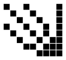
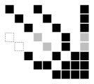
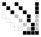
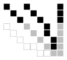
Figure 2: Illustration of Step 2 (row-reduction process) of Algorithm 1 for the tree in Figure 1. The matrix represents $[A\;|\;c]$. The black squares represent unchanged non-zero values of $A$ and the grey squares represent non-zero values that are updated at some iteration in Step 2. In the final matrix (far right), the values in the last column are the values assigned to the vector $C$ in Steps 1 and 2 above, while the remaining columns that form an upper triangular matrix are the values corresponding to the constructed $P$ matrix. The backward solve of Step 3 solves the linear system.

To illustrate the message-passing algorithm in the terminology of Gaussian elimination, we first need to divide the nodes $\{1,2,\dots,n\}$ in the forest into sets $L\{1\}$, $L\{2\},\dots,L\{T\}$, where $L\{1\}$ is an arbitrary node in the graph $G$ selected to be the “root” node, $L\{2\}$ is the set of all neighbours of the “root” node, $L\{3\}$ is the set of all neighbours of the nodes in $L\{2\}$ excluding parent nodes (nodes in $L\{1\!:\!2\}$), and so on until all nodes are assigned to a set (if the forest is made of disconnected trees, we will need to do this for each tree). An example of this process is depicted in Figure 1. Once these sets are initialized, we start with the nodes furthest from the root node(s) $L\{T\}$, and carry out the row operations of Gaussian elimination moving towards the root. Then we use backward substitution to solve the system $Ax=c$. We outline the full procedure in Algorithm 1 and illustrate the algorithm on a particular example in Figure 2.

5.3 Forest-Structured BCD Updates

To illustrate how being able to solve forest-structured linear systems in linear time can be used within BCD methods, consider the basic quadratic minimization problem

$$\mathop{\hbox{arg\,min}}_{x\in{\rm I\!R}^{n}}\frac{1}{2}x^{T}Ax-c^{T}x,$$

where we assume the matrix $A\in{\rm I\!R}^{n\times n}$ is positive-definite and sparse. By excluding terms not depending on the coordinates in the block, the optimal update for block $b$ is given by the solution to the linear system

$$A_{bb}x_{b}=\tilde{c},$$ (26)

where $A_{bb}\in{\rm I\!R}^{|b|\times|b|}$ is the submatrix of $A$ corresponding to block $b$, and $\tilde{c}=c_{b}-A_{b\bar{b}}x_{\bar{b}}$ is a vector with $\bar{b}$ defined as the complement of $b$ and $A_{b\bar{b}}\in{\rm I\!R}^{|b|\times|\bar{b}|}$ is the submatrix of $A$ with rows from $b$ and columns from $\bar{b}$. We note that in practice efficient BCD methods will typically track $Ax$ (to implement the iterations efficiently) so computing $\tilde{c}$ is efficient.

The graph obtained from the sub-matrix $A_{bb}$ is called the induced subgraph $G_{b}$ of the original graph $G$. Specifically, the nodes $V_{b}\in G_{b}$ are the coordinates in the set $b$, while the edges $E_{b}\in G_{b}$ are all edges $(i,j)\in E$ where $i,j\in V_{b}$ (edges between nodes in $b$). Even if the original problem is not a forest-structured graph, we can choose the block $b$ so that the induced subgraph $G_{b}$ is forest-structured. Using blocks constructed in this way, we can compute the optimal update (26) in linear time using message passing as described in the previous seciton.

For non-quadratic problems, the optimal update is not the solution of a linear system. Nevertheless, we can choose blocks so that the induced subgraph is forest-structured and use message-passing to efficiently compute matrix updates (which leads to a linear system involving $H_{b}$) or Newton updates (which leads to a linear system involving the sub-Hessian). We note that similar ideas have recently been explored by Srinivasan and Todorov (2015) for Newton methods. Their graphical Newton algorithm can solve the Newton system in $O(t^{3})$ times the size of $G$, where $t$ is the “treewidth” of the graph ($t=1$ and the graph size is at most linear for forests). However, the tree-width of $G$ is usually large while it is more reasonable to assume that we can find low-treewidth induced subgraphs $G_{b}$.

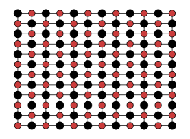
(a) Red-black, $|b|=n/2$.

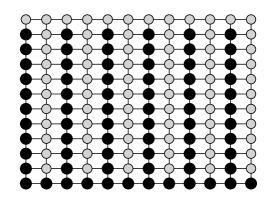
(b) Fixed block, $|b|=n/2$.

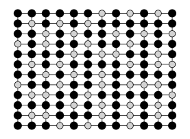
(c) Variable block, $|b|\approx 2n/3$.

Figure 3: Partitioning strategies for defining forest-structured blocks.

Whether or not message-passing is useful will depend on the sparsity pattern of $A$. For example, if $A$ is dense then we may only be able to choose forest-structured induced-subgraphs of size 2. On the other hand, if $A$ is diagonal then this would correspond to a disconnected graph, which is clearly a forest and would allow an optimal BCD update with a block size of $n$ (so we would solve a quadratic problem in 1 iteration). As an example between these extremes, consider a quadratic function with a lattice-structured non-zero pattern as in Figure 3. This graph is a bipartite graph (“two-colourable”), and a classic fixed partitioning strategy for problems with this common structure is to use a “red-black ordering” (see Figure 3a). Choosing this colouring makes the matrix $A_{bb}$ diagonal when we update the red nodes, allowing us to solve (26) in linear time (and similarly for the black nodes). So this colouring scheme allows an $O(n)$-time optimal BCD update with a block size of $n/2$, rather than the $O(n^{3})$-time required for the optimal update of an arbitrary block of size $n/2$.

Message passing allows us to go beyond the red-black colouring, and instead update any forest-structured block of size $\tau$ in linear time. For example, the partition given in Figure 3b also has blocks of size $n/2$, but these blocks include dependencies. Our experiments indicate that blocks that maintain dependencies, such as Figure 3b, make substantially more progress than using the red-black blocks or using small non-forest-structured blocks (though red-black blocks are very well-suited for parallelization).

Alternatively, we can consider variable blocks with forest-structured induced subgraphs, where the block size may vary at each iteration, but restricting to forests still leads to a linear-time update. As seen in Figure 3c, by allowing variable block sizes we can select a forest-structured block of size $|b|\approx 2n/3$ in one iteration (black nodes) while still maintaining a linear-time update. If we further sample different random forests or blocks at each iteration, then the convergence rate under this strategy is covered by the arbitrary sampling theory (Qu et al., 2015). Also note that the maximum of the gradient norms over all forests defines a valid norm, so our analysis of Gauss-Southwell can be applied to this case.

5.4 From Red-Black to Multi-Colourings

The adjacency matrix in the red-black example is called “consistently ordered” in the numerical linear algebra literature, meaning that the nodes can be partitioned into sets such that any two adjacent nodes belong to different sets (Young, 1971, Def. 5.3.2). A matrix being consistently-ordered is equivalent to the graph being “two-colourable” in the language of graph theory: each node can be assigned one of two colours, such that no adjacent nodes receive the same colour. We can generalize the red-black approach to arbitrary graphs by defining our blocks such that no two neighbours are in the same block. While for lattice-structured graphs we only need two blocks to do this, for general graphs we may need a larger number of blocks. This is called a multi-colouring in the numerical linear algebra literature (Harrar, 1993; Saad, 2003, §12.4), and may lead to blocks of different sizes. If a graph is $\nu$-colourable, then we can arrange the adjacency matrix such that it has $\nu$ diagonal blocks along its diagonal (the off-diagonal blocks may be dense). In relation to BCD methods, this means that $A_{bb}$ is diagonal for each block and we can update each of the $\nu$ blocks in linear time in the size of the block.

Finding the minimum number of “colours” (number of blocks) for a given graph is exactly the graph colouring problem, which is NP-hard (Garey and Johnson, 1979). However, there are various heuristics that quickly give a (potentially non-minimal) valid colouring of the nodes (for a survey of heuristic, meta-heuristic, and hybrid methods for graph colouring, see Baghel et al. (2013)). For example, in our experiments we used the following classic greedy algorithm (Welsh and Powell, 1967):

1. Proceed through the vertices of the graph in some order $i=1,2,\dots,n$.

2. For each vertex $i$, assign it the smallest positive integer (“colour”) such that it does not have the same colour as any of its neighbours among the vertices $\{1,2,\dots,i-1\}$.

We can use all vertices assigned to the same integer as our blocks in the algorithm, and if we apply this algorithm to a lattice-structured graph (using row- or column-ordering of the nodes) then we obtain the classic red-black colouring of the graph.

5.5 Partitioning into Forest-Structured Blocks

Instead of disconnected blocks, in this work we instead consider forest-structured blocks. The size of the largest possible forest is also related to the graph colouring problem (Esperet et al., 2015), and we can consider a slight variation on the second step of the greedy colouring algorithm to find a set of forest-structured blocks:

1. Proceed through the vertices of the graph in some order $i=1,2,\dots,n$.

2. For each vertex $i$, assign it the smallest positive integer (“forest”) such that the nodes assigned to that integer among the set $\{1,2,\dots,i\}$ form a forest.

If we apply this to a lattice-structured graph (in column-ordering), this generates a partition into two forest-structured graphs similar to the one in Figure 3b (only the bottom row is different). This procedure requires us to be able to test whether adding a node to a forest maintains the forest property, and we show how to do this efficiently in Appendix D.

In the case of lattice-structured graphs there is a natural ordering of the vertices, but for many graphs there is no natural ordering. In such cases we might simply consider a random ordering. Alternately, if we know the individual Lipschitz constants $L_{i}$, we could order by these values (with the largest $L_{i}$ going first so that they are likely assigned to the same block if possible). In our experiments we found that this ordering improved performance for an unstructured dataset, and performed similarly to using the natural ordering in a lattice-structured dataset.

5.6 Approximate Greedy Rules with Forest-Structured Blocks

Similar to the problems of the previous section, computing the Gauss-Southwell rule over forest-structured variable blocks is NP-hard, as we can reduce the 3-satisfiability problem to the problem of finding a maximum-weight forest (Garey and Johnson, 1979). However, we use a similar greedy method to approximate the greedy Gauss-Southwell rule over the set of trees:

1. Initialize $b_{k}$ with the node $i$ corresponding to the largest gradient, $|\nabla_{i}f(x^{k})|$.

2. Search for the node $i$ with the largest gradient that is not part of $b_{k}$ and that maintains that $b_{k}$ is a forest.

3. If such a node is found, add it to $b_{k}$ and go back to step 2. Otherwise, stop.

Although this procedure does not yield the exact solution in general, it is appealing since (i) the procedure is efficient as it is easy to test whether adding a node maintains the forest property (see Appendix D), (ii) it outputs a forest so that the subsequent update is linear-time, (iii) we are guaranteed that the coordinate corresponding to the variable with the largest gradient is included in $b_{k}$ (guaranteeing convergence), and (iv) we cannot add any additional node to the final forest and still maintain the forest property. A similar heuristic can be used to approximate the GSD rule under the restriction from Section 4.1 or to generate a forest randomly.

6 Manifold Identification

The previous section advocated the use of Newton updates over matrix updates, where feasible. We usually associate Newton updates with superlinear convergence as opposed to linear convergence. However, updating blocks of variables destroys the possibility for superlinear convergence even in settings where Newton’s method would achieve superlinear convergence. In this section, we consider non-smooth problems where in some settings an appropriate block selection strategy combined with Newton updates of the blocks does lead to superlinear convergence.

In paritcular, we consider optimization problems of the form

$$\mathop{\hbox{arg\,min}}_{x\in{\rm I\!R}^{n}}f(x)+\sum_{i=1}^{n}g_{i}(x_{i}),$$ (27)

where $\nabla f$ is Lipschitz-continuous and each $g_{i}$ only needs to be convex and lower semi-continuous (it may be non-smooth or infinite at some $x_{i}$). A classic example of a problem in this framework is optimization subject to non-negative constraints,

$$\mathop{\hbox{arg\,min}}_{x\geq 0}f(x),$$ (28)

where in this case $g_{i}$ is the indicator function on the non-negative orthant,

$$g_{i}(x_{i})=\begin{cases}0&\text{if }x_{i}\geq 0,\\ \infty&\text{if }x_{i}<0.\end{cases}$$

Another example that has received significant recent attention is the case of an L1-regularizer,

$$\mathop{\hbox{arg\,min}}_{x\in{\rm I\!R}^{n}}f(x)+\lambda\|x\|_{1},$$ (29)

where in this case $g_{i}=\lambda|x_{i}|$. Here, the L1-norm regularizer is used to encourage sparsity in the solution. A related problem is the group L1-regularization problem (7), where instead of being separable, $g$ is block-separable.

Proximal gradient methods have become one of the default strategies for solving problem (27), and a BCD variant of these methods has an update of the form

$$x^{k+1}=\hbox{prox}_{\alpha_{k}g_{b_{k}}}\left[x^{k}-\alpha_{k}U_{b_{k}}\nabla_{b_{k}}f(x^{k})\right],$$ (30)

where for any block $b$ and step-size $\alpha$ the proximal operator is defined by the separable optimization

$$\hbox{prox}_{\alpha g_{b}}[x]=\mathop{\hbox{arg\,min}}_{y\in\mathbb{R}^{n}}\frac{1}{2\alpha}\|y-x\|^{2}+\sum_{i\in b}g_{i}(y_{i}).$$

We note that all variables not in block $b$ stay at their existing values in the optimal solution to this problem. In the special case of non-negative constraints like (28) the update in (30) is given by

$$x_{i}^{k+1}=\left[x_{i}-\frac{1}{L}\nabla_{i}f(x^{k})\right]^{+},$$

where $[\beta]^{+}=\max\{0,\beta\}$ projects onto the non-negative orthant. For L1-regularization problems (29) the update reduces to an element-wise soft-thresholding step,

$$x_{i}^{k+\frac{1}{2}} =x^{k}-\frac{1}{L}\nabla_{i}f(x^{k}),$$ (31)

$$x_{i}^{k+1} ={\color[rgb]{0,0,0}\text{sgn}(x_{i}^{k+\frac{1}{2}})}\left[\left|x_{i}^{k+\frac{1}{2}}\right|-\frac{\lambda}{L}\right]^{+},$$

which we have written as a gradient update followed by the soft-threshold operator. Here, the signum function sgn$(x_{i})$ returns $1$ if $x_{i}$ is positive, returns -1 if it is negative, and can return any number between $-1$ and $1$ if $x_{i}$ is zero.

Most of the issues discussed in the previous sections for smooth BCD methods carry over in a straightforward way to this proximal setting; we can still consider fixed or variable blocks, there exist matrix and Newton updates, and we can still consider cyclic, random, or greedy selection rules. One subtle issue is that there are many generalizations of the Gauss-Southwell rule to the proximal setting (Nutini et al., 2015). However, the GS-$q$ rule defined by Tseng and Yun (2009b) seems to be the generalization of GS with the best theoretical properties. A GSL variant of this rule would take the form

$$b_{k}\in\mathop{\hbox{arg\,min}}_{b\in\mathcal{B}}\left\{\min_{d}\left\{\langle\nabla_{b}f(x^{k}),d\rangle+\frac{L_{b}}{2}\|d\|^{2}+\sum_{i\in b}g_{i}(x_{i}+d_{i})-\sum_{i\in b}g_{i}(x_{i})\right\}\right\},$$ (32)

where we assume that the gradient of $f$ is $L_{b}$-Lipschitz continuous with respect to block $b$. A generalization of the GS rule is obtained if we assume that the $L_{b}$ are equal across all blocks. We can similarly define a GSD-$q$ and GSQ-$q$ rule by using

$$b_{k}\in\mathop{\hbox{arg\,min}}_{b\in\mathcal{B}}\left\{\min_{d}\left\{\langle\nabla_{b}f(x^{k}),d\rangle+\frac{1}{2}\|d\|_{H_{b}}^{2}+\sum_{i\in b}g_{i}(x_{i}+d_{i})-\sum_{i\in b}g_{i}(x_{i})\right\}\right\},$$ (33)

where the gradient of block $b$ is $1-$Lipschitz continuous with respect to the quadratic norm defined by the matrix $H_{b}$ (GSD-$q$ would correspond to the special case where the $H_{b}$ are diagonal). Convergence of this method under standard assumptions follows existing arguments (Tseng and Yun, 2009a, b; Csiba and Richtárik, 2017).

It has been established that coordinate descent and BCD methods based on the update (30) for problem (27) obtain similar convergence rates to the case where we do not have a non-smooth term $g$ (Nesterov, 2012; Richtárik and Takáč, 2014; Nutini et al., 2015). The focus of this section is to show that the non-smoothness of $g$ can actually lead to a faster convergence rate.

This idea dates back at least 40 years to the work of Bertsekas (1976). For the case of non-negative constraints, he shows that the sparsity pattern of $x^{k}$ generated by the projected-gradient method matches the sparsity pattern of the solution $x^{*}$ for all sufficiently large $k$. Thus, after a finite number of iterations the projected-gradient method will “identify” the final set of non-zero variables. Once these values are identified, Bertsekas suggests that we can fix the zero-valued variables and apply an unconstrained Newton update to the set of non-zero variables to obtain superlinear convergence. Even without switching to a superlinearly-convergent method, the convergence rate of the projected-gradient method can be faster once the set of non-zeroes is identified since it is effectively optimizing in the lower-dimensional space corresponding to the non-zero variables.

This idea of identifying a smooth “manifold” containing the solution $x^{*}$ has been generalized to allow polyhedral constraints (Burke and Moré, 1988), general convex constraints (Wright, 1993), and even non-convex constraints (Hare and Lewis, 2004). Similar results exist in the proximal gradient setting. For example, it has been shown that the proximal gradient method identifies the sparsity pattern in the solution of L1-regularized problems after a finite number of iterations (Hare, 2011). The active-set identification property has also been shown for other algorithms like certain coordinate descent and stochastic gradient methods (Mifflin and Sagastizábal, 2002; Wright, 2012; Lee and Wright, 2012). Specifically, Wright shows that BCD also has this manifold identification property for separable $g$ (Wright, 2012), provided that the coordinates are chosen in an essentially-cyclic way (or provided that we can simultaneously choose to update all variables that do not lie on the manifold). Wright also shows that superlinear convergence is possible if we use a Newton update on the manifold, assuming the Newton update does not leave the manifold.

In the next subsection, we present a manifold identification result for proximal coordinate descent for general separable $g$. We follow a similar argument to Bertsekas (1976), which yields a simple proof that holds for many possible selection rules including greedy rules (which may not be essentially-cyclic). Further, our argument leads to bounds on the active-set complexity of the method, which is the number of iterations required to reach the manifold (Liang et al., 2017; Nutini et al., 2019). As examples, we consider problems (28) and (29), and show explicit bounds for the active-set complexity. We subsequently show how to generalize this argument to cases like block updates and Newton updates. The latter naturally leads to superlinear convergence of greedy BCD methods when using variable blocks of size larger than the dimension of the manifold.

6.1 Manifold Identification for Separable $g$

Assume the subdifferential of $g$ is nonempty for all $x\in\!\hbox{{ dom\;}}{(g)}$. By our separability assumption on $g$, the subdifferential of $g$ can be expressed as the concatenation of the individual subdifferential of each $g_{i}$, where the subdifferential of $g_{i}$ at any $x_{i}\in{\rm I\!R}$ is defined by

$$\partial g_{i}(x_{i})=\{v\in{\rm I\!R}:g_{i}(y)\geq g_{i}(x_{i})+v\cdot(y-x_{i}),\text{ for all $y\in\!\hbox{{ dom\;}}{(g_{i})}$}\}.$$

This implies that the subdifferential of each $g_{i}$ is just an interval on the real line. In particular, the interior of the subdifferential of each $g_{i}$ at a non-differentiable point $x_{i}$ can be written as an open interval,

$$\mathop{\hbox{int}}\partial g_{i}(x_{i})\equiv(l_{i},u_{i}),$$ (34)

where $l_{i}\in{\rm I\!R}\cup\{-\infty\}$ and $u_{i}\in{\rm I\!R}\cup\{\infty\}$ (the $\infty$ values occur if $x_{i}$ is at its lower or upper bound, respectively). The active-set at a solution $x^{*}$ for a separable $g$ is then defined by

$$\mathcal{Z}=\{i:\partial g_{i}(x_{i}^{*})\text{ is not a singleton}\}.$$

By (34), the set $\mathcal{Z}$ includes indices $i$ where $x_{i}^{*}$ is equal to the lower bound on $x_{i}$, is equal to the upper bound on $x_{i}$, or occurs at a non-smooth value of $g_{i}$. In our examples of non-negative constraints or L1-regularization, $\mathcal{Z}$ is the set of coordinates that are zero at the solution $x^{*}$. With this definition, we can formally define the manifold identification property.

Definition 4

The manifold identification property for problem (27) is satisfied if for all sufficiently large $k$, we have that $x_{i}^{k}=x_{i}^{*}$ for some solution $x^{*}$ for all $i\in\mathcal{Z}$.

In order to prove the manifold identification property for the proximal coordinate descent method, in addition to assuming that $\nabla f$ is $L$-Lipschitz continuous, we require two assumptions. Our first assumption is that the iterates of the algorithm converge to a solution $x^{*}$.

Assumption 1

The iterates of the proximal coordinate descent method converge to an optimal solution $x^{*}$ of problem (27), that is $x^{k}\to x^{*}$ as $k\to\infty$.

This assumption holds if $f$ is strongly-convex and if we use cyclic or greedy selection (see Appendix E), but will also hold under a variety of other scenarios. Our second assumption is a nondegeneracy condition on the solution $x^{*}$ that the algorithm converges to. Below we write the standard nondegeneracy condition from the literature for the special case of (27).

Assumption 2

We say that $x^{*}$ is a nondegenerate solution for problem  (27) if it holds that

$$\begin{cases}-\nabla_{i}f(x^{*})=\nabla_{i}g(x^{*}_{i})&\text{if $\partial g_{i}(x_{i}^{*})$ is a singleton ($g_{i}$ is smooth at $x_{i}^{*}$)}\\ -\nabla_{i}f(x^{*})\in\mathop{\hbox{int}}\partial g_{i}(x^{*}_{i})&\text{if $\partial g_{i}(x_{i}^{*})$ is not a singleton ($g_{i}$ is non-smooth at $x_{i}^{*}$)}.\end{cases}$$

This condition states that $-\nabla f(x^{*})$ must be in the “relative interior” (see Boyd and Vandenberghe, 2004, Section 2.1.3) of the subdifferential of $g$ at the solution $x^{*}$. In the case of the non-negative bound constrained problem (28), this requires that $\nabla_{i}f(x^{*})>0$ for all variables $i$ that are zero at the solution ($x_{i}^{*}=0$). For the L1-regularization problem (29), this requires that $|\nabla_{i}f(x^{*})|<\lambda$ for all variables $i$ that are zero at the solution.

There are three results that we require in order to prove the manifold identification property. The first result follows directly from Assumption 1 and establishes that for any $\beta>0$ there exists a finite iteration $\bar{k}$ such that the distance from the iterate $x^{k}$ to the solution $x^{*}$ for all iterations $k\geq\bar{k}$ is bounded above by $\beta$.

Lemma 5

Let Assumption 1 hold. For any $\beta$, there exists some minimum finite $\bar{k}$ such that $\|x^{k}-x^{*}\|\leq\beta$ for all $k\geq\bar{k}$.

The second result we require is that for any $i\in\mathcal{Z}$ such that $x_{i}^{k}\not=x_{i}^{*}$, eventually coordinate $i$ is selected at some finite iteration.

Lemma 6

Let Assumption 1 hold. If $x_{i}^{k}\not=x^{*}_{i}$ for some $i\in\mathcal{Z}$, then coordinate $i$ will be selected by the proximal coordinate descent method after a finite number of iterations.

Proof  For eventual contradiction, suppose we did not select such an $i$ after iteration $k^{\prime}$. Then for all $k\geq k^{\prime}$ we have that

$$|x_{i}^{k^{\prime}}-x_{i}^{*}|=|x_{i}^{k}-x_{i}^{*}|\leq\|x^{k}-x^{*}\|.$$ (35)

By Assumption 1 the right-hand side is converging to 0, so it will eventually be less than $|x_{i}^{k^{\prime}}-x^{*}_{i}|$ for some $k\geq k^{\prime}$, contradicting the inequality. Thus after a finite number of iterations we must have that $x_{i}^{k}\neq x_{i}^{k^{\prime}}$, which can only be achieved by selecting $i$.  

The third result we require is that once Lemma 5 is satisfied for some finite $\bar{k}$ and a particular $\beta>0$, then for any coordinate $i\in\mathcal{Z}$ selected at some iteration $k^{\prime}\geq\bar{k}$ by the proximal coordinate descent method, we have $x^{k^{\prime}}_{i}=x^{*}_{i}$. We prove that this happens for a value $\beta$ depending on a quantity $\delta$ defined by

$$\delta=\min_{i\in\mathcal{Z}}\left\{\min\{-\nabla_{i}f(x^{*})-l_{i},u_{i}+\nabla_{i}f(x^{*})\}\right\},$$ (36)

which is the minimum distance to the nearest boundary of the subdifferential (34) among indices $i\in\mathcal{Z}$.

Lemma 7

Consider problem (27), where $f$ is convex with $L$-Lipschitz continuous gradient and the $g_{i}$ are proper convex functions (not necessarily smooth). Let Assumptions 1 be satisfied and Assumption 2 be satisfied for the particular $x^{*}$ that the algorithm converges to. Then for the coordinate-wise proximal-gradient iteration (30) with a step-size of $1/L$, if $\|x^{k}-x^{*}\|\leq\delta/2L$ holds and $i\in\mathcal{Z}$ is selected at iteration $k$, then $x_{i}^{k+1}=x^{*}_{i}$.

Proof  We obtain this result by applying (Nutini et al., 2019, Lemma 1), but restricting the function to the coordinate being updated.  
With the above results we next have the manifold identification property.

Theorem 8

Consider problem  (27), where $f$ is convex with $L$-Lipschitz continuous gradient and the $g_{i}$ are proper convex functions. Let Assumptions 1 be satisfied and Assumption 2 be satisfied for the particular $x^{*}$ that the algorithm converges to. Then for the coordinate-wise proximal-gradient iteration (30) a step-size of $1/L$, there exists a finite $k$ such that $x_{i}^{k}=x_{i}^{*}$ for all $i\in\mathcal{Z}$.

Proof  Lemma 5 implies that the assumptions of Lemma 7 are eventually satisfied, and combining this with Lemma 6 we have the result.  

Both problems (28) and (29) satisfy the manifold identification result. By the definition of $\delta$ in (36), we have that $\delta=\min_{i\in\mathcal{Z}}\{\nabla_{i}f(x^{*})\}$ for problem (28). We note that if $\delta=0$, then we may approach the manifold through the interior of the domain and the manifold may never be identified (this is the purpose of the nondegeneracy condition). For problem (29), we have that $\delta=\lambda-\max_{i\in\mathcal{Z}}\{|\nabla_{i}f(x^{*})|\}$. From these results, we are able to define explicit bounds on the number of iterations required to reach the manifold, a new result that we explore in the next subsection.

Instead of using a step-size of $1/L$, it is more common to use a bigger step-size of $1/L_{i}$ within coordinate descent methods, where $L_{i}$ is the coordinate-wise Lipschitz constant. In this case, the results of Lemma 7 hold for $\beta=\delta/(L+L_{i})$. This is a larger region since $L_{i}\leq L$, so with this standard step-size the iterates can move onto the manifold from further away and we expect to identify the manifold earlier. The argument can also be modified to use other step-size selection methods, provided that we can write the algorithm in terms of a step-size $\alpha_{k}$ that is guaranteed to be bounded from below. While the above result considers single-coordinate updates, it can trivially be modified to show that BCD with larger block sizes (and gradient updates) have the manifold identification property. The only change is that once $\|x^{k}-x^{*}\|\leq\delta/2L$, we have that $x_{i}^{k+1}=x_{i}^{*}$ for all $i\in b_{k}\cap\mathcal{Z}$. Thus, BCD methods can simultaneously move many variables onto the optimal manifold.

6.2 Active-Set Complexity

The manifold identification property of the previous section could also be shown using the more sophisticated tools used in related works (Burke and Moré, 1988; Hare and Lewis, 2004). However, an appealing aspect of the simple argument above is that it can be combined with non-asymptotic convergence rates of the iterates to bound the number of iterations required to reach the manifold. This was first explored by Liang et al. (2017) and we call this the “active-set complexity” of the method. We have recently given tighter bounds than Liang et al. on the active-set complexity of proximal-gradient methods for strongly-convex objectives (Nutini et al., 2019). Here we use a similar analysis to bound the active-set complexity of BCD methods, which is complicated by the fact that not all coordinates are updated on each iteration.

We will consider the active-set complexity in the case where $f$ is strongly-convex and we use cyclic or greedy selection. This guarantees that

$$\|x^{k}-x^{*}\|\leq\left(1-\frac{1}{\kappa}\right)^{k}\gamma,$$ (37)

for some $\gamma\geq 0$ and some $\kappa\geq 1$ (see Appendix E, and we note that this type of rate also holds for a variety of other types of selection rules). By using that $(1-1/\kappa)^{k}\leq\exp(-k/\kappa)$, the linear convergence rate (37) implies the following result on how many iterations it will take to identify the active-set, and thus reach the manifold.

Theorem 9

Consider any method that achieves an iterate bound (37). For $\delta$ as defined in (36), we have $\|x^{\bar{k}}-x^{*}\|\leq\delta/2L$ after at most $\kappa\log(2L\gamma/\delta)$ iterations. Further, we will identify the active-set after an additional $t$ iterations, where $t$ is the number of additional iterations required to select all suboptimal $x_{i}$ with $i\in\mathcal{Z}$ as part of some block.

Proof  See Corollary 1 in Nutini et al. (2019) for bounding the time until we are “close” to the solution, in the sense that $\|x^{\bar{k}}-x^{*}\|\leq\delta/2L$. It then follows from applying Nutini et al. (2019, Lemma 1) that each time a suboptimal $x_{i}$ with $i\in\mathcal{Z}$ is selected that it will set $x_{i}^{k}=x_{i}^{*}$. Thus, by how $t$ is defined, we will identify the active-set $t$ iterations after we become “close” to the solution.  
The value of $t$ depends on the selection rule we use. If we use cyclic selection we will require at most $t=n$ additional iterations to select all suboptimal coordinates $i\in\mathcal{Z}$ and thus to reach the optimal manifold. To bound the active-set complexity for general rules like greedy rules, we cannot guarantee that all coordinates will be selected after $n$ iterations once we are close to the solution. In the case of non-negative constraints, the number of additional iterations depends on a quantity we will call $\epsilon$, which is the smallest non-zero variable $x_{i}^{\bar{k}}$ for $i\in\mathcal{Z}$ and $\bar{k}$ satisfying the first part of Theorem 9. It follows from (37) that we require at most $\kappa\log(\gamma/\epsilon)$ iterations beyond $\bar{k}$ to select all non-zero $i\in\mathcal{Z}$. Thus, the active-set complexity for greedy rules for problem (28) is bounded above by $\kappa(\log(2L\gamma/\delta)+\log(\gamma/\epsilon))$. Based on this bound, greedy rules (which yield a smaller $\kappa$) may identify the manifold more quickly than cyclic rules in cases where $\epsilon$ is large. However, if $\epsilon$ is very small then greedy rules may take a larger number of iterations to reach the manifold.

6.3 Proximal-Newton Updates and Superlinear Convergence

Once we have identified the optimal manifold, we can think about switching from using the proximal BCD method to using an unconstrained optimizer on the coordinates $i\not\in\mathcal{Z}$. The unconstrained optimizer can be a Newton update, and thus under the appropriate conditions can achieve superlinear convergence. However, a problem with such “2-phase” approaches is that we do not know the exact time at which we reach the optimal manifold. This can make the approach inefficient: if we start the second phase too early, then we sub-optimize over the wrong manifold, while if we start the second phase too late, then we waste iterations performing first-order updates when we should be using second-order updates. Wright proposes an interesting alternative where at each iteration we consider replacing the gradient proximal-BCD update with a Newton update on the current manifold (Wright, 2012). This has the advantage that the manifold can continue to be updated, and that Newton updates are possible as soon as the optimal manifold has been identified. However, note that the dimension of the current manifold might be larger than the block size and the dimension of the optimal manifold, so this approach can significantly increase the iteration cost for some problems.

Rather than “switching” to an unconstrained Newton update, we can alternately take advantage of the superlinear converge of proximal-Newton updates (Lee et al., 2012). For example, in this section we consider Newton proximal-BCD updates as in several recent works (Qu et al., 2016; Tappenden et al., 2016; Fountoulakis and Tappenden, 2018). For a block $b$ these updates have the form

$$x_{b}^{k+1}\in\mathop{\hbox{arg\,min}}_{y\in\mathbb{R}^{|b|}}\left\{\langle\nabla_{b}f(x_{b}^{k}),y-x_{b}^{k}\rangle+\frac{1}{2\alpha_{k}}\|y-x_{b}^{k}\|_{H_{b}^{k}}^{2}+\sum_{i\in b}g_{i}(y_{i})\right\},$$ (38)

where $H_{b}^{k}$ is the matrix corresponding to block $b$ at iteration $k$ (which can be the sub-Hessian $\nabla_{bb}^{2}f(x^{k})$). This is a generalization of the matrix update (5), and that update is obtained in the special case where the $g_{i}$ are constant. As before if we set $H_{b}^{k}=H_{b}$ for some fixed matrix $H_{b}$, then we can take $\alpha_{k}=1$ if block $b$ of $f$ is 1-Lipschitz continuous in the $H_{b}$-norm. Alternately, if we set $H_{b}^{k}=\nabla_{b_{k},b_{k}}^{2}f(x^{k})$ then we obtain a generalization of Newton’s method.

In the next section, we give a practical variant on proximal-Newton updates that also has the manifold identification property under standard assumptions. An advantage of this approach is that the block size typically restricts the computational complexity of the Newton update (which we discuss further in the next sections). Further, superlinear convergence is possible in the scenario where the coordinates $i\not\in\mathcal{Z}$ are chosen as part of the block $b_{k}$ for all sufficiently large $k$. However, note that this superlinear scenario only occurs in the special case where we use a greedy rule with variable blocks and where the size of the blocks is at least as large as the dimension of the optimal manifold. With variable blocks, the GS-$q$ and GSL-$q$ rules (32) or GSD-$q$ and GSQ-$q$ rules (33) will no longer select coordinates $i\in\mathcal{Z}$ since their optimal $d_{i}$ value is zero when close to the solution and on the manifold. Thus, these rules will only select $i\not\in\mathcal{Z}$ once the manifold has been identified. In contrast, we would not expect superlinear convergence for fixed blocks unless all $i\not\in\mathcal{Z}$ happen to be in the same partition. While we could show superlinear convergence of subsequences for random selection with variable blocks, the number of iterations between elements of the subsequence may be prohibitively large.

6.4 Practical Proximal-Newton Methods

A challenge with using the update (38) in general is that the optimization is non-quadratic (due to the $g_{i}$ terms) and non-separable (due to the $H_{b}^{k}$-norm). If we make the $H_{b}^{k}$ diagonal, then the objective is separable, but this destroys the potential for superlinear convergence. Fortunately, a variety of strategies exist in the literature to allow non-diagonal $H_{b}^{k}$.

For example, for bound constrained problems we can apply two-metric projection (TMP) methods, which use a modified $H_{b}^{k}$ and allow the computation of a (cheap) projection under the Euclidean norm (Gafni and Bertsekas, 1984). This method splits the coordinates into an “active-” set and a “working-” set, where the active-set $\mathcal{A}$ for non-negative constraints would be

$$\mathcal{A}=\{i~{}|~{}x_{i}<\epsilon,\nabla_{i}f(x)>0\},$$

for some small $\epsilon$ while the working-set $\mathcal{W}$ is the compliment of this set. So the active-set contains the coordinates corresponding to the variables that we expect to be zero while the working-set contains the coordinates corresponding to the variables that we expect to be unconstrained. The TMP method can subsequently use the update

$$x_{\mathcal{W}} \leftarrow\hbox{proj}_{C}\left(x_{\mathcal{W}}-\alpha H_{\mathcal{W}}^{-1}\nabla_{\mathcal{W}}f(x)\right)$$

$$x_{\mathcal{A}} \leftarrow\hbox{proj}_{C}\left(x_{\mathcal{A}}-\alpha\nabla_{\mathcal{A}}f(x)\right).$$

This method performs a gradient update on the active-set and a Newton update on the working-set. Gafni and Bertsekas (1984) show that this preserves many of the essential properties of projected-Newton methods like giving a descent direction, converging to a stationary point, and superlinear convergence if we identify the correct set of non-zero variables. Also note that for indices $i\in\mathcal{Z}$, this eventually only takes gradient steps so our analysis of the previous section applies (it identifies the manifold in a finite number of iterations). As opposed to solving the block-wise proximal-Newton update in (38), in our experiments we explored simply using the TMP update applied to the block and found that it gave nearly identical performance.

TMP methods have also been generalized to settings like L1-regularization (Schmidt, 2010) and they can essentially be used for any separable $g$ function. Another widely-used strategy is to inexactly solve (38) (Schmidt, 2010; Lee et al., 2012; Fountoulakis and Tappenden, 2018). This has the advantage that it can still be used in the group L1-regularization setting or other group-separable settings.

6.5 Optimal Updates for Quadratic $f$ and Piecewise-Linear $g$

Two of the most well-studied optimization problems in machine learning are the SVM and LASSO problems. The LASSO problem is given by an L1-regularized quadratic objective

$$\mathop{\hbox{arg\,min}}_{x}\frac{1}{2}\|Ax-b\|^{2}+\lambda\|x\|_{1},$$

while the dual of the (non-smooth) SVM problem has the form of a bound-constrained quadratic objective

$$\mathop{\hbox{arg\,min}}_{0\leq x\leq\gamma}\frac{1}{2}x^{T}Ax,$$

for some matrix $A$ (positive semi-definite in the SVM case), and regularization constants $\lambda$ and $\gamma$. In both cases we typically expect the solution to be sparse, and identifying the optimal manifold has been shown to improve practical performance of BCD methods (Joachims, 1999; De Santis et al., 2016).

Both problems have a set of $g_{i}$ that are piecewise-linear over their domain, implying that the they can be written as a maximum over univariate linear functions on the domain of each variable. Although we can still consider TMP or inexact proximal-Newton updates for these problems, this special structure actually allows us to compute the exact minimum with respect to a block (which is efficient when considering medium-sized blocks). Indeed, for SVM problems the idea of using exact updates in BCD methods dates back to the sequential minimal optimization (SMO) method (Platt, 1998), which uses exact updates for blocks of size 2. In this section we consider methods that work for blocks of arbitrary size.

While we could write the optimal update as a quadratic program, the special structure of the LASSO and SVM problems lends well to exact homotopy methods. These methods date back to Osborne et al. (2000); Osborne and Turlach (2011) who proposed an exact homotopy method that solves the LASSO problem for all values of $\lambda$. This type of approach was later popularized under the name “least angle regression” (LARS) (Efron et al., 2004). Since the solution path is piecewise-linear, given the output of a homotopy algorithm we can extract the exact solution for our given value of $\lambda$. Hastie et al. (2004) derive an analogous homotopy method for SVMs, while Rosset and Zhu (2007) derive a generic homotopy method for the case of piecewise-linear $g_{i}$ functions.

The cost of each iteration of a homotopy method on a problem with $|b|$ variables is $O(|b|^{2})$. It is known that the worst-case runtime of these homotopy methods can be exponential (Mairal and Yu, 2012). However, the problems where this arises are somewhat unstable, and in practice the solution is typically obtained after a linear number of iterations. This gives a runtime in practice of $O(|b|^{3})$, which does not allow enormous blocks, but does allow us to efficiently use block sizes in the hundreds or thousands. That being said, since these methods compute the exact block update, in the scenario where we previously had superlinear convergence, we now obtain finite convergence. That is, the algorithm will stop in a finite number of iterations with the exact solution provided that it has identified the optimal manifold, uses a greedy rule with variable blocks, and the block size is larger than the dimension of the manifold. This finite termination is also guaranteed under similar assumptions for TMP methods, and although TMP methods may make less progress per-iteration than exact updates, they may be a cheaper alternative to homotopy methods as the cost is explicitly restricted to $O(|b|^{3})$.

7 Numerical Experiments

We performed an extensive variety of experiments to evaluate the effects of the choices listed in the previous sections. In this section we include several of these results that highlight some key trends we observed, and in each subsection below we explicitly list the insights we obtained from the experiment. We considered five datasets that evaluate the methods in a variety of scenarios:

1. Least-squares with a sparse data matrix (10,000 variables).

2. Binary logistic regression with a sparse data matrix (10,000 variables).

3. 50-class logistic regression problem with a sparse data matrix (50,000 variables).

4. Lattice-structured quadratic objective as in Section 5 (2,400 variables).

5. Binary label propagation problem (sparse but unstructured quadratic) (1,900 variables).

We give the full details of these datasets in Appendix F where we have also included our full set of experiment results. Due to the sparsity present in these datasets, it is possible to implement the basic GS rule for a similar cost to random selection (by tracking the gradient element in a max-heap structure). We used the bounds in Appendix B to set the various Lipschitz constants ($L_{i}$, $L_{b}$, and $H_{b}$).

In our experiments we use the number of iterations as our measure of performance. This measure is far from perfect, especially when considering greedy methods, since it ignores the computational cost of each iteration. However, this measure of performance provides an implementation- and problem-independent measure of performance. We seek an implementation-independent measure of performance since the actual runtimes of different methods will vary wildly across applications. However, it is typically easy to estimate the per-iteration runtime when considering a new problem. Thus, we hope that our quantification of what can be gained from faster-converging methods gives guidance to readers about whether the faster-converging methods will lead to a substantial performance gain on their applications. We are careful to qualify all of our claims with warnings in cases where the iteration costs differ.

7.1 Greedy Rules with Gradient Updates

Our first experiment considers gradient updates with a step-size of $1/L_{b}$, and seeks to quantify the effect of using fixed blocks compared to variable blocks (Section 3.1) as well as the effect of using the new block GSL rule (Section 3.2). In particular, we compare selecting the block using Cyclic, Random, Lipschitz (sampling the elements of the block proportional to $L_{i}$), GS, and GSL rules. For each of these rules we implemented a fixed block (FB) and variable block (VB) variant. For VB using Cyclic selection, we split a random permutation of the coordinates into equal-sized blocks and updated these blocks in order (followed by using another random permutation). We also considered Perm with FB, where we use a fixed set of blocks and we go through a sequence of random permutations of these blocks. To approximate the seemingly-intractable GSL rule with VB, we used the GSD rule (Section 3.4) using the SIRT-style approximation (23) from Section 4.1. To construct the partition of the coordinates needed in the FB method, we sorted the coordinates according to their $L_{i}$ values then placed the largest $L_{i}$ values into the first block, the next set of largest in the second block, and so on. Since quite a few methods are being compared, we list the full set of methods used in this experiment (as well as the experiment of the next section) in Table 1.

		Blocking Strategy
		Fixed (FB)	Variable (VB)
Block Selection Rule	Cyclic $b=1,2,\dots,n/\tau,1,2,\dots$	Cyclic-FB:       sort $L_{i}$, group into equal sized       blocks, cycle through blocks in order	Cyclic-VB:       randomly permute $i$, group into equal       sized blocks, cycle through blocks in order,       repeat
	Random $b\in\{1,2,\dots,n/\tau\}$	Random-FB:       sort $L_{i}$, group into equal sized blocks,       select blocks uniformly at random	Random-VB:       select $\tau$ coordinates uniformly at random at       each iteration
	Lipschitz Sampling $p(b_{k}=b)=\frac{L_{b}}{\sum_{\hat{b}\in\mathcal{B}}L_{\hat{b}}}$	Lipschitz-FB:       sort $L_{i}$, group into equal sized blocks,       select blocks randomly according to       non-uniform distribution	Lipschitz-VB:       select $\tau$ coordinates randomly according to       non-uniform distribution, $p_{i}=L_{i}/\sum_{i=1}^{n}L_{i}$
	Gauss-Southwell (GS) $\displaystyle b_{k}\in\mathop{\hbox{arg\,max}}_{b\in\mathcal{B}}\|\nabla_{b}f(x^{k})\|$	GS-FB:       sort $L_{i}$, group into equal sized blocks,       select blocks using GS rule	GS-VB:       select the $\tau$ maximal coordinates according       to the single-coordinate GS rule
	Gauss-Southwell-Lipschitz (GSL) $\displaystyle b_{k}\in\mathop{\hbox{arg\,max}}_{b\in\mathcal{B}}\left\{\frac{\|\nabla_{b}f(x^{k})\|^{2}}{L_{b}}\right\}$	GSL-FB:       sort $L_{i}$, group into equal sized blocks,       select blocks using GSL rule	GSL-VB:       select the $\tau$ maximal coordinates according       to the GSD rule ($D_{b,i}=D_{i}$), use SIRT       to compute the $D_{i}$ (4.1)
	Gauss-Southwell-Diagonal (GSD) $\mathop{\hbox{arg\,max}}_{b\in\mathcal{B}}\left\{\sum_{i\in b}\frac{|\nabla_{i}f(x^{k})|^{2}}{D_{b,i}}\right\}$	GSD-FB:       sort $L_{i}$, group into equal sized blocks,       select blocks using GSD rule ($D_{b,i}=L_{i}$)	GSD-VB:       select the $\tau$ maximal coordinates according       to the GSD rule ($D_{b,i}=L_{i}$)
	Gauss-Southwell-Quadratic (GSQ) $\displaystyle b_{k}\in\mathop{\hbox{arg\,max}}_{b\in\mathcal{B}}\left\{\|\nabla_{b}f(x^{k})\|_{H_{b}^{-1}}\right\}$	GSQ-FB:       sort $L_{i}$, group into equal sized blocks,       select blocks using GSQ rule	GSQ-VB:       use approximation to GSQ rule (4.2)       and 10 iterations of IHT

Table 1: Summary of block selection rules and blocking strategies used in Figures 4 & 5.

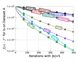
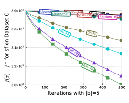
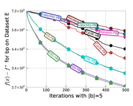
Figure 4: Comparison of cyclic, random and greedy block selection rules using either FB or VB with a gradient update on three different problems. We see that the greedy selection rules tend to make more progress than the cyclic or random selection rules. Further, the greedy VB variations can converge substantially faster than greedy FB, and the GSL rule can converge substantially faster than the classic GS rule. Details on the full set of methods used in this experiment are in Table 1.

We plot selected results for a block size of 5 in Figure 4, while experiments on all datasets and with other block sizes are given in Appendix F.2. Overall, we observed the following trends regarding the number of iterations:

• Greedy rules tend to make more progress per iteration than random and cyclic rules, particularly with small block sizes. This difference is sometimes enormous, and this suggests we should prefer greedy rules when the greedy rules can be implemented with a similar cost to cyclic or random selection.

• The variance of the performance between the rules becomes smaller as the block size increases. This is because the performance of all methods increases with the block size, and suggests that if we use very-large block sizes with gradient updates that we should prefer simple Cyclic or Random updates.

• VB can converge substantially faster than FB when using GS for certain problems. This agrees with the theory, because the FBs are a subset of the VBs so the progress bound for VBs always dominates FBs. Thus, we should prefer GS-VB for problems where this has a similar cost to GS-FB. We found this trend was reversed for random rules, where fixed blocks tended to perform better. We suspect this trend is due to the coupon collector problem: with random selection it takes FB fewer iterations than VB to select all variables at least once.

• GSL can converge substantially faster than the classic GS rule for certain problems (while the performance was always at least as good). In some cases the new block-GSL rule with FB even outperformed the GS rule with VB. Interestingly, the prior work evaluating the single-coordinate GSL rule only showed minor practical gains for GSL over GS (Nutini et al., 2015), while in the block case the performance gain was in some cases much larger.

In Appendix F.2 we repeat this experiment for the FB methods but using the approximation to $L_{b}$ discussed in Section 4.3 (see Figure 9). This sought to test whether this procedure, which may underestimate the true $L_{b}$ and thus use larger step-sizes, would improve performance. This experiment lead to some additional insights:

• Approximating $L_{b}$ was more effective as the block size increases. This makes sense, since with large block sizes there are more possible directions and we are unlikely to ever need to use a step-size as small as $1/L_{b}$ for the global $L_{b}$ (which increases with block size).

• Approximating $L_{b}$ is far more effective than using a loose bound. For small block sizes we have relatively-good bounds for all problems except Problem C. On this problem the Lipschitz approximation procedure was much more effective even for small block sizes.

• GSL sometimes performed worse than the classic GS rule when approximating $L_{b}$. This seems sensible, particularly early in the optimization, since the GS rule does not depend on the $L_{b}$ while the GSL rule can potentially be negatively affected by poor estimates of $L_{b}$. This suggests that, for example, we might want to consider methods that start out using the GS rule and gradually switch to using the GSL rule.

This experiment suggests that we should prefer to use an approximation to $L_{b}$ (or an explicit line-search) when using gradient updates unless we have a tight approximation to the true $L_{b}$ and we are using a small block size. We also performed experiments with different block partitioning strategies when using greedy rules with FB (see Figure 10). In those experiments, our sorting approach tended to outperform using random blocks or choosing the blocks to have similar average Lipschitz constants.

7.2 Greedy Rules with Matrix Updates

Our next experiment considers using matrix updates based on the matrices $H_{b}$ from Appendix B, and quantifies the effects of the GSQ and GSD rules introduced in Sections 3.3-3.4 as well the approximations to these introduced in Sections 4.1-4.2. In particular, for FB we consider the GS rule and the GSL rule (from the previous experiment), the GSD rule (using the diagonal matrices from Section 4.1 with $D_{b,i}=L_{i}$), and the GSQ rule (which is optimal for the three quadratic objectives). For VB we consider the GS rule from the previous experiment as well as the GSD rule (using $D_{b,i}=L_{i}$), and the GSQ rule using the approximation from Section 4.2 and 10 iterations of iterative hard thresholding. Other than switching to matrix updates and focusing on these greedy rules, we keep all other experimental factors the same.

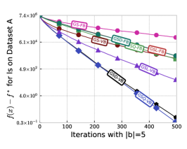
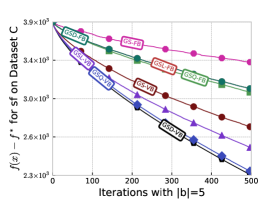
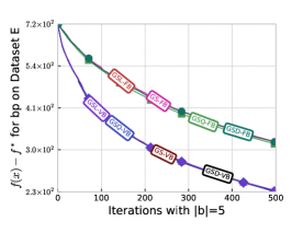
Figure 5: Comparison of different greedy block selection rules using either FB or VB with matrix updates on three different problems. For all methods considered, the VB variations consistently performed similar or better than the FB variations in terms of convergence rate. We see that even using the crude approximation for GSD with VB ($D_{b,i}=L_{i}$), it often outperforms GS-VB and GSL-VB. Details on the full set of methods used in this experiment are in Table 1.

We plot selected results of doing this experiment in Figure 5. These experiments showed the following interesting trends:

• There is a larger advantage to VB in terms of convergence rate with matrix updates. When using matrix updates, the basic GS-VB method converged faster than even the most effective GSQ-FB rule for smaller block sizes.

• With FB, there is little advantage to GSD/GSQ. Although the GSL rule consistently improved over the classic GS rule, we did not see any advantage to using the more-advanced GSD or GSQ rules when using FB.

• GSD can converge substantially faster than the classic GS rule with VB for certain problems (while the performance was always at least as good). Despite the use of a crude diagonal approximation, the GSD rule often outperformed the classic GS rule. The GSD-VB method (which uses $D_{{\color[rgb]{0,0,0}b},i}=L_{i}$) also consistently performed similar or better than the GSL-VB method (which uses a different diagonal scaling with a tighter bound), despite the GSL-VB having better performance when using gradient updates.

• GSQ converged slightly faster than GSD with VB and large blocks. Although the GSQ-VB rule performed the best across all experiments in terms of number of iterations, the difference was more noticeable for large block sizes. However, this did not offset its high cost in any experiment. We also experimented with OMP instead of IHT, and found it gave a small improvement, but the iterations were substantially more expensive.

Putting the above together, with matrix updates our experiments indicate that among greedy rules the GSD rule seems to provide good performance in all settings. We would only recommend using the GSQ rule in settings where we can use VB and where operations involving the objective $f$ are much more expensive than running an IHT or OMP method. We performed experiments with different block partition strategies for FB, but found that when using matrix updates the partitioning strategy did not make a big difference for cyclic, random, or greedy rules.

In Appendix F.3 we repeat this experiment for the non-quadratic objectives using the Newton direction and a backtracking line-search to set the step-size (see Figure 12), as discussed in Sections 4.4 and 4.6. For both datasets, the Newton updates resulted in faster convergence than the matrix updates. This indicates that we should prefer classic Newton updates over the more recent matrix updates for non-quadratic objectives where computing the sub-block of the Hessian is tractable.

7.3 Message-Passing Updates

We next seek to quantify the effect of using message-passing to efficiently implement exact updates for quadratic functions, as discussed in Section 5. For this experiment, we focused on the lattice-structured dataset D and the unstructured but sparse dataset E. These are both quadratic objectives with high treewidth, but that allow us to find large forest-structured induced subgraphs. We compared the following strategies to choose the block: greedily choosing the best general unstructured blocks using GS (General), cycling between blocks generated by the greedy graph colouring algorithm of Section 5.4 (Red Black), cycling between blocks generated by the greedy forest-partitioning algorithm of Section 5.5 (Tree Partitions), greedily choosing a tree using the algorithm of Section 5.6 (Greedy Tree), and growing a tree randomly using the same algorithm (Random Tree). For the lattice-structured Dataset D, the partitioning algorithms (for Red Black and Tree Partitions) proceed through the variables in order which generates partitions similar to those shown in Figure 3b. For the unstructured Dataset E, we apply the partitioning strategies of Section 5.5 using both a random ordering (Random) and by sorting the Lipschitz constants $L_{i}$ (Lipschitz). Since the cost of the exact update for tree-structured methods is $O(n)$, for the unstructured blocks we chose a block size of $b_{k}=n^{1/3}$ to make the costs comparable (since the exact solve is cubic in the block size for unstructured blocks). In Table 2, we list the full set of methods used in Figure 6.

		Blocking Strategy
Block Selection Rule	General	Select the best general unstructured block using the GS-VB rule from 1.
	Random Tree	Grow a tree randomly using the algorithm of Section 5.6.
	Greedy Tree	Greedily choose a tree using the algorithm of Section 5.6.
	Red Black	Cycle between blocks generated by the greedy graph colouring algorithm of Section 5.4. This requires choosing an ordering of the variables. For the lattice-structured data we used a colum-major ordering. For the unstructured data we considered two approaches: Random: Use a random order. Lipschitz: Proceed through the vertices by descending Lipschitz values.
	Tree Partitions	Cycle between blocks generated by the greedy forest-partitioning algorithm of Section 5.5. This requires choosing an ordering of the variables. For the lattice-structured data we used a colum-major ordering. For the unstructured data we considered two approaches: Random: Use a random order. Lipschitz: Proceed through the vertices by descending Lipschitz values.

Table 2: Summary of blocking strategies used in Figure 6. For the algorithms used for Red Black and Tree Partitions blocking strategies, we consider three variations of ordering strategies in Step 1.

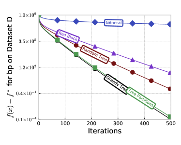
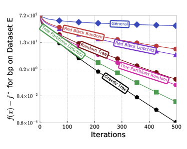
Figure 6: Comparison of different blocking strategies on two quadratic graph-structured problems when using optimal updates. While the Random Tree blocking strategy performed better than the Red Black method, overall the Greedy Tree and Tree Partitions strategies performed best on these structured problems. We note that cycling through the vertices according to descending Lipschitz values for Red Black and Tree Partitions gives us better results than cycling through the vertices in random order. Details on the full set of methods used in this experiment are in Table 2.

We plot selected results of doing this experiment in Figure 6. Here, we see that even the classic red-black ordering outperforms using general unstructured blocks (since general blocks must use such small block sizes). The tree-structured blocks perform even better, and in the unstructured setting our greedy approximation of the GS rule under variable blocks converges faster than the other strategies. However, our greedy tree partitioning method also performs well. For the lattice-structured data it converged at a similar rate to the greedy approximation, while for the unstructured data it converged faster than all methods except greedy (and performed better when sorting by the Lipschitz constants than using a random order).

7.4 Proximal Updates

Our final experiment demonstrates the manifold identification and superlinear/finite convergence properties of the greedy BCD method as discussed in Section 6 for a sparse non-negative constrained L1-regularized least-squares problem using Dataset A. In particular, we compare the performance of a projected gradient update with $L_{b}$ step-size, a projected Newton (PN) solver with line-search as discussed in Section 6.3 and the two-metric projection (TMP) update as discussed in Section 6.4 when using fixed (FB) and variable (VB) blocks of different sizes ($|b|\in\{5,50,100\}$). We use a regularization constant of $\lambda=50,000$ to encourage a high level of sparsity resulting in an optimal solution $x^{*}$ with 51 non-zero variables. In Figure 7 we indicate active-set identification with a star and show that all approaches eventually identify the active-set. We see that TMP converges at nearly the same speed as projected Newton for all block sizes (despite its lower iteration cost) and both converge faster than performing gradient updates. For a block size of 100, we get finite convergence using projected Newton and TMP updates. In Table 3, we list details for each method used in Figure 7.

			Blocking Strategy
		Update Formula	Fixed (FB)	Variable (VB)
Block Update Rule	Projected Gradient (PG)	$x_{b}^{k+1}=\left[x_{b}-\frac{1}{L_{b}}\nabla_{b}f(x^{k})\right]^{+}$	PG-FB:       sort $L_{i}$, group into equal sized blocks, select blocks using GSL-q rule	PG-VB:       select the $\tau$ maximal coordinates according to the GSD-q rule       with $D_{b,i}=L_{i}$
	Projected Newton (PN)	Solve quadratic program, see (38) (using line-search from Section 6.3)	PN-FB:       sort $L_{i}$, group into equal sized blocks, select blocks using GSL-q rule	PN-VB:       select the $\tau$ maximal coordinates       according to the GSD-q rule       with $D_{b,i}=L_{i}$
	Two-Metric Projection (TMP)	Solve linear system and project, see Section 6.4	TMP-FB:       sort $L_{i}$, group into equal sized blocks, select blocks using GSL-q rule	TMP-VB:       select the $\tau$ maximal coordinates       according to the GSD-q rule       with $D_{b,i}=L_{i}$

Table 3: Summary of block update rules used in Figure 7.

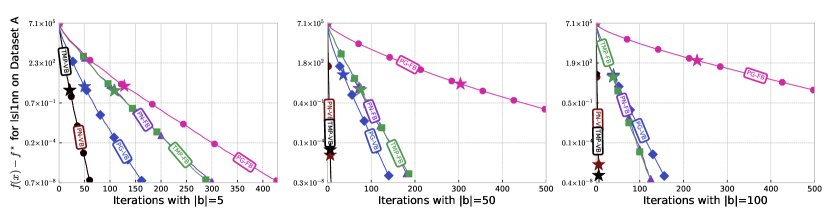
Figure 7: Comparison of different proximal updates when using greedy fixed and variable blocks of different sizes. The star on each curve indicates active-set identification. We see that TMP and projected Newton converge faster than using gradient updates, while TMP achieves a similar convergence speed as projected Newton despite having a lower iteration cost. Further, the VB variations consistently outperformed all the FB variations, except for the largest block size of 100, where TMP-FB and PN-FB beat PG-VB. Details for each method used in this experiment are in Table 3.

In Appendix F.4 we repeat this experiment for random block selection and show that for such a sparse problem multiple iterations are often required before progress is made due to the repetitive selection of variables that are already zero/active.

8 Discussion

An important issue that we have not discussed is how to choose the block size $\tau$. BCD tends to converge faster with larger blocks, but this must be balanced against the higher iteration cost of using larger blocks. In some cases the blocks are dictated by a certain problem structure such as group L1-regularization where the objective is block separable or multi-class logistic regression where updating a suitable block has the same cost as updating a single coordinate. As a practical recommendation, we suggest choosing the largest block size where we can still view the update as “inexpensive”. This is because it is typically easy to estimate iteration costs in practice while predicting the convergence rate in practice is more difficult. As an example, if the cost of the update is $O(\tau^{3})$ then blocks of size 5 might be preferred over blocks of size 1 while blocks of size 10000 could lead to an unnacceptably slow iteration cost.

In this work we focused on non-accelerated BCD methods. However, we expect that our conclusions are likely to also apply for accelerated BCD methods (Fercoq and Richtárik, 2015). We thus expect this work to be complimentary to recent work on accelerated greedy coordinate descent methods (Locatello et al., 2018; Lu et al., 2018). Similarly, while we focused on the setting of serial computation, we expect that our conclusions will give insight into developing more efficient parallel and distributed BCD methods (Richtárik and Takáč, 2016).

Although our experiments indicate that our choice of the diagonal matrices $D$ within the GSD rule provides a consistent improvement, this choice is clearly sub-optimal. A future direction is to find a generic strategy to construct better diagonal matrices, and work on ESO methods could potentially be adapted for doing this (Qu and Richtárik, 2016). This could be in the setting where we are given knowledge of the Lipschitz constants, but a more-interesting idea is to construct these matrices online as the algorithm runs.

The GSQ rule can be viewed as a greedy rule that incorporates more sophisticated second-order information than the simpler GS and GSL rules. In preliminary experiments, we also considered selection rules based on the cubic regularization bound. However, these did not seem to converge more quickly than the existing rules in our experiments, and it is not obvious how one could efficiently implement such second-order rules.

We focused on BCD methods that approximate the objective function at each step by globally bounding higher-order terms in a Taylor expansion. However, we would expect more progress if we could bound these locally in a suitably-larger neighbourhood of the current iteration. Alternately, note that bounding the Taylor expansion is not the only way to upper bound a function. For example, Khan (2012) discusses a variety of strategies for bounding the binary logistic regression loss and indeed proves that other bounds are tighter than the Taylor expansion (“Böhning”) bound that we use. It would be interesting to explore the convergence properties of BCD methods whose bounds do not come from a Taylor expansion.

While we focused on the case of trees, there are message-passing algorithms that allow graphs with cycles (Rose, 1970; Srinivasan and Todorov, 2015). The efficiency of these methods depends on the “treewidth” of the induced subgraph, where if the treewidth is small (as in trees) then the updates are efficient, and if the treewidth is large (as in fully-connected graphs) then these do not provide an advantage. Treewidth is related to the notion of “chordal” graphs (trees are special cases of chordal graphs) and chordal embeddings which have been exploited for matrix problems like covariance estimation (Dahl et al., 2008) and semidefinite programming (Sun et al., 2014; Vandenberghe and Andersen, 2015). Considering “treewidth 2” or “treewidth 3” blocks would give more progress than our tree-based updates, although it is NP-hard to compute the treewidth of a general graph (but it is easy to upper-bound this quantity by simply choosing a random elimination order).

As opposed to structural constraints like requiring the graph to be a tree, it is now known that message-passing algorithms can solve linear systems with other properties like diagonal dominance or “attractive” coefficients (Malioutov et al., 2006). There also exist specialized linear-time solvers for Laplacian matrices (Kyng and Sachdeva, 2016), and these can be used within BCD methods for certain structures. It would also be interesting to explore whether approximate message-passing algorithms which allow general graphs (Malioutov et al., 2006) can be used to improve optimization algorithms.

Acknowledgments

We would like to thank Dr. Warren Hare for fruitful conversations that helped with Section 6. We would also like to thank Francis Bach, Coralia Cartis, Aleksandar Dogandzic, Chen Greif, Ives Macedo, Anastasia Podosinnikova, Suvrit Sra, and the anonymous reviewers for valuable discussions and feedback. This work was supported by a Discovery Grant from the Natural Sciences and Engineering Research Council of Canada (NSERC). Julie Nutini and Issam Laradji are funded by UBC Four-Year Doctoral Fellowships (4YFs).

Appendix Appendix A Cost of Multi-Class Logistic Regression

The typical setting where we expect coordinate descent to outperform gradient descent is when the cost of one gradient descent iteration is similar to the cost of updating all variables via coordinate descent. It is well known that for the binary logistic regression objective, one of the most ubiquitous models in machine learning, coordinate descent with uniform random selection satisfies this property. We previously showed that this property is also satisfied for the GS rule in the case of logistic regression, provided that the data is sufficiently sparse (Nutini et al., 2015).

In this section we consider multi-class logistic regression. We first analyze the cost of gradient descent on this objective and how randomized coordinate descent is efficient for any sparsity level. Then we show that a high sparsity level is not sufficient for the GS rule to be efficient for this problem, but that it is efficient if we use a particular set of fixed blocks.

Appendix A.1 Cost of Gradient Descent

The likelihood for a single training example $i$ with features $a_{i}\in{\rm I\!R}^{d}$ and a label $b_{i}\in\{1,2,\dots,k\}$ is given by

$$p(b_{i}\;|\;a_{i},X)=\frac{\exp(x_{b_{i}}^{T}a_{i})}{\sum_{c=1}^{k}\exp(x_{c}^{T}a_{i})},$$

where $x_{c}$ is column $c$ of our matrix of parameters $X\in{\rm I\!R}^{d\times k}$ (so the number of parameters $n$ is $dk$). To maximize the likelihood over $m$ independent and identically-distributed training examples we minimize the negative log-likelihood,

$$f(X)=\sum_{i=1}^{m}\left[-x_{b_{i}}^{T}a_{i}+\log\left(\sum_{c=1}^{k}\exp(x_{c}^{T}a_{i})\right)\right],$$ (39)

which is a convex function. The partial derivative of this objective with respect to a particular $X_{jc}$ is given by

$$\frac{\partial}{\partial X_{jc}}f(X) =-\sum_{i=1}^{m}a_{ij}\left[I(b_{i}=c)-\frac{\exp(x_{c}^{T}a_{i})}{\sum_{c^{\prime}=1}^{k}\exp(x_{c^{\prime}}^{T}a_{i})}\right],$$ (40)

where $I$ is a $0/1$ indicator variable and $a_{ij}$ is feature $j$ for training example $i$. We use $A$ to denote a matrix where row $i$ is given by $a_{i}^{T}$. To compute the full gradient, the operations which depend on the size of the problem are:

1. Computing $x_{c}^{T}a_{i}$ for all values of $i$ and $c$.

2. Computing the sums $\sum_{c=1}^{k}\exp(x_{c}^{T}a_{i})$ for all values of $i$.

3. Computing the partial derivative sums (40) for all values of $j$ and $c$.

The first step is the result of the matrix multiplication $AX$, so if $A$ has $z$ non-zeroes then this has a cost of $O(zk)$ if we compute it using $k$ matrix-vector multiplications. The second step costs $O(mk)$, which under the reasonable assumption that $m\leq z$ (since each row usually has at least one non-zero) is also in $O(zk)$. The third step is the result of a matrix multiplication of the form $A^{T}R$ for a (dense) $m$ times $k$ matrix $R$ (whose elements have a constant-time cost to compute given the results of the first two steps), which also costs $O(zk)$ giving a final cost of $O(zk)$.

Appendix A.2 Cost of Randomized Coordinate Descent

Since there are $n=dk$ variables, we want our coordinate descent iterations to be $dk$-times faster than the gradient descent cost of $O(zk)$. Thus, we want to be able to implement coordinate descent iterations for a cost of $O(z/d)$ (noting that we always expect $z\geq d$ since otherwise we could remove some columns of $A$ that only have zeroes). The key to doing this for randomized coordinate descent is to track two quantities:

1. The values $x_{c}^{T}a_{i}$ for all $i$ and $c$.

2. The values $\sum_{c^{\prime}=1}^{k}\exp(x_{c^{\prime}}^{T}a_{i})$ for all $i$.

Given these values we can compute the partial derivative in $O(z/d)$ in expectation, because this is the expected number of non-zero values of $a_{ij}$ in the partial derivative sum (40) ($A$ has $z$ total non-zeroes and we are randomly choosing one of the $d$ columns). Further, after updating a particular $X_{jc}$ we can update the above quantities for the same cost:

1. We need to update $x_{c}^{T}a_{i}$ for the particular $c$ we chose for the examples $i$ where $a_{ij}$ is non-zero for the chosen value of $j$. This requires an $O(1)$ operation (subtract the old $x_{jc}a_{ij}$ and add the new value) for each non-zero element of column $j$ of $A$. Since $A$ has $z$ non-zeroes and $d$ columns, the expected number of non-zeroes is $z/d$ so this has a cost of $O(z/d)$.

2. We need to update $\sum_{c^{\prime}=1}^{k}\exp(x_{c^{\prime}}^{T}a_{i})$ for all $i$ where $a_{ij}$ is non-zero for our chosen $j$. Since we expect $z/d$ non-zero values of $a_{ij}$, the cost of this step is also $O(z/d)$.

Note that BCD is also efficient since if we update $\tau$ elements, the cost is $O(z\tau/d)$ by just applying the above logic $\tau$ times. In fact, the second step and computing the final partial derivative has some redundant computation if we update multiple $X_{jc}$ with the same $c$, so we might have a small performance gain in the block case.

Appendix A.3 Cost of Greedy Coordinate Descent (Arbitrary Blocks)

The cost of greedy coordinate descent is typically higher than randomized coordinate descent since we need to track all partial derivatives. However, consider the case where each row has at most $z_{r}$ non-zeroes and each column has at most $z_{c}$ non-zeroes. In this setting we previously showed that for binary logistic regression it is possible to track all partial derivatives for a cost of $O(z_{r}z_{c})$, and that we can track the maximum gradient value at the cost of an additional logarithmic factor (Nutini et al., 2015, Appendix A). Thus, greedy coordinate selection has a similar cost to uniform selection when the sparsity pattern makes $z_{r}z_{c}$ similar to $z/d$ (as in the case of a grid-structured dependency graph like Figure 3).

Unfortunately, having $z_{r}z_{c}$ similar to $z/d$ is not sufficient in the multi-class case. In particular, the cost of tracking all the partial derivatives after updating an $X_{jc}$ in the multi-class case can be broken down as follows:

1. We need to update $x_{c}^{T}a_{i}$ for the examples $i$ where $a_{ij}$ is non-zero. Since there are at most $z_{c}$ non-zero values of $a_{ij}$ over all $i$ the cost of this is $O(z_{c})$.

2. We need to update $\sum_{c=1}^{k}\exp(x_{c}^{T}a_{i})$ for all $i$ where $a_{ij}$ is non-zero. Since there are at most $z_{c}$ non-zero values of $a_{ij}$ the cost of this is $O(z_{c})$.

3. We need to update the partial derivatives $\partial f/\partial X_{jc}$ for all $j$ and $c$. Observe that each time we have $a_{ij}$ non-zero, we change the partial derivative with respect to all features $j^{\prime}$ that are non-zero in the example $i$ and we must update all classes $c^{\prime}$ for these examples. Thus, for the $O(z_{c})$ examples with a non-zero feature $j$ we need to update up to $O(z_{r})$ other features for that example and for each of these we need to update all $k$ classes. This gives a cost of $O(z_{r}z_{c}k)$.

So while in the binary case we needed $O(z_{r}z_{c})$ to be comparable to $O(z/d)$ for greedy coordinate descent to be efficient, in the multi-class case we now need $O(z_{r}z_{c}k)$ to be comparable to $O(z/d)$ in the multi-class case. This means that not only do we need a high degree of sparsity but we also need the number of classes $k$ to be small for greedy coordinate descent to be efficient for arbitrary blocks.

Appendix A.4 Cost of Greedy Coordinate Descent (Fixed Blocks)

Greedy rules are more expensive in the multi-class case because whenever we change an individual variable $X_{jc}$, it changes the partial derivative with respect to $X_{j^{\prime}c^{\prime}}$ for a set of $j^{\prime}$ values and for all $c^{\prime}$. However, we can improve the efficiency of greedy rules by using a special choice of fixed blocks that reduces the number of $j^{\prime}$ values. In particular, BCD is more efficient for the multi-class case if we put $X_{jc^{\prime}}$ for all $c^{\prime}$ into the same block. In other words, we ensure that each row of $X$ is part of the same block so that we apply BCD to rows rather than in an unstructured way. Below we consider the cost of updating the needed quantities after changing an entire row of $X_{jc}$ values:

1. Since we are updating $k$ elements, the cost of updating the $x_{c}^{T}a_{i}$ is $k$-times larger giving $O(z_{c}k)$ when we update a row.

2. Similarly, the cost of updating the sums $\sum_{c=1}^{k}\exp(x_{c}^{T}a_{i})$ is $k$-times larger also giving $O(z_{c}k)$.

3. Where we gain in computation is the cost of computing the changed values of the partial derivatives $\partial f/\partial X_{jc}$. As before, each time we have $a_{ij}$ non-zero for our particular row $j$, we change the partial derivative with respect to all other $j^{\prime}$ for this example and with respect to each class $c^{\prime}$ for these $j^{\prime}$. Thus, for the $O(z_{c})$ examples with a non-zero feature $j$ we need to update up to $O(z_{r})$ other features for that example and for each of these we need to update all $k$ classes. However, since $j$ is the same for each variable we update, we only have to do this once which gives us a cost of $O(z_{r}z_{c}k)$.

So the cost to update a row of the matrix $X$ is $O(z_{r}z_{c}k)$, which is the same cost as only updating a single element. Considering the case of updating individual rows, this gives us $d$ blocks so in order for BCD to be efficient it must be $d$-times faster than the gradient descent cost of $O(zk)$. Thus, we need a cost of $O(zk/d)$ per iteration. This is achieved if $O(z_{r}z_{c})$ to be similar to $O(z/d)$, which is the same condition we needed in the binary case.

Appendix Appendix B Blockwise Lipschitz Constants

In this section we show how to derive lower-bounds on the block-Lipschitz constants of the gradient and Hessian for several common problem settings. We will use that a twice-differentiable function has an $L$-Lipschitz continuous gradient if and only if the absolute eigenvalues of its Hessian are upper-bounded by $L$,

$$\|\nabla f(x)-\nabla f(y)\|\leq L\|x-y\|\iff\nabla^{2}f(x)\preceq LI.$$

This implies that when considering blockwise constants we have

$$\|\nabla_{b}f(x+U_{b}d)-\nabla_{b}f(x)\|\iff\nabla_{bb}^{2}f(x)\preceq L_{b}I,$$

for some $L_{b}\leq L$. Thus, bounding the blockwise eigenvalues of the Hessian bounds the blockwise Lipschitz constants of the gradient. We also use that this equivalence extends to the case of general quadratic norms,

$$\|\nabla_{b}f(x+U_{b}d)-\nabla_{b}f(x)\|_{H_{b}^{-1}}\leq\|d\|_{H_{b}}\iff\nabla_{bb}^{2}f(x)\preceq H_{b}.$$

Appendix B.1 Quadratic Functions

Convex quadratic functions have the form

$$f(x)=\frac{1}{2}x^{T}Ax+c^{T}x,$$

for a positive semi-definite matrix $A$ and vector $c$. For all $x$ the Hessian with respect to block $b$ is given by the sub-matrix of $A$,

$$\nabla_{bb}^{2}f(x)=A_{bb}.$$

Thus, we have that $L_{b}$ is given by the maximum eigenvalue of the submatrix, $L_{b}=\|A_{b}\|$ (the operator norm of the submatrix). In the special case where $b$ only contains a single element $i$, we have that $L_{i}$ is given by the absolute value of the diagonal element, $L_{i}=|A_{ii}|$. If we want to use a general quadratic norm we can simply take $H_{b}=A_{bb}$, which is cheaper to compute than the $L_{b}$ (since it does not require an eigenvalue calculation).

Appendix B.2 Least Squares

The least squares objective has the form

$$f(x)=\frac{1}{2}\|Ax-c\|^{2},$$

for a matrix $A$ and vector $c$. This is a special case of a quadratic function, where the Hessian is given by

$$\nabla^{2}f(x)=A^{T}A.$$

This gives us that $L_{b}=\|A_{b}\|^{2}$ (where $A_{b}$ is the matrix containing the columns $b$ of $A$). In the special case where the block has a single element $j$, observe that $L_{j}=\sum_{i=1}^{m}a_{ij}^{2}$ (sum of the squared values in column $j$) so we do not need to solve an eigenvalue problem. When using a quadratic norm we can take $H_{b}=A_{b}^{T}A_{b}$ which similarly does not require solving an eigenvalue problem.

Appendix B.3 Logistic Regression

The likelihood of a single example in a logistic regression model is given by

$$p(b_{i}\;|\;a_{i},x)=\frac{1}{1+\exp(-b_{i}x^{T}a_{i})},$$

where each $a_{i}\in{\rm I\!R}^{d}$ and $b_{i}\in\{-1,1\}$. To maximize the likelihood over $m$ examples (sampled independently) we minimize the negative log-likelihood,

$$f(x)=\sum_{i=1}^{m}\log(1+\exp(-b_{i}x^{T}a_{i})).$$

Using $A$ as a matrix where row $i$ is given by $a_{i}^{T}$ and defining $h_{i}(x)=p(b_{i}\;|\;a_{i},x)$, we have that

$$\nabla^{2}f(x) =\sum_{i=1}^{m}h_{i}(x)(1-h_{i}(x))a_{i}a_{i}^{T}$$

$$\preceq 0.25\sum_{i=1}^{m}a_{i}a_{i}^{T}$$

$$=0.25A^{T}A.$$

The generalized inequality above is the binary version of the bound of Böhning (1992). This bound can be derived by observing that $h_{i}(x)$ is in the range $(0,1)$, so the quantity $h_{i}(x)(1-h_{i}(x))$ has an upper bound of $0.25$. This result means that we can use $L_{b}=0.25\|A_{b}\|^{2}$ for block $b$, $L_{j}=0.25\sum_{i=1}^{m}a_{ij}^{2}$ for single-coordinate blocks, and $H_{b}=0.25A_{b}^{T}A_{b}$ if we are using a general quadratic norm (notice that computing $H_{b}$ is again cheaper than computing $L_{b}$).

Appendix B.4 Multi-Class Logistic Regression

The Hessian of the multi-class logistic regression objective (39) with respect to parameter vectors $x_{c}$ and $x_{c^{\prime}}$ can be written as

$$\frac{\partial^{2}}{\partial x_{c}\partial x_{c^{\prime}}}f(X)=\sum_{i=1}^{m}h_{i,c}(X)(I(c=c^{\prime})-h_{i,c^{\prime}}(X))a_{i}a_{i}^{T},$$

where similar to the binary logistic regression case we have defined $h_{i,c}=p(c\;|\;a_{i},X)$. This gives the full Hessian the form

$$\nabla^{2}f(X) =\sum_{i=1}^{m}H_{i}(X)\otimes a_{i}a_{i}^{T},$$

where we used $\otimes$ to denote the Kronecker product and where element $(c,c^{\prime})$ of the $k$ by $k$ matrix $H_{i}(X)$ is given by $h_{i,c}(X)(I(c=c^{\prime})-h_{i,c^{\prime}}(X))$. The bound of Böhning (1992) on this matrix is that

$$H_{i}(X)\preceq\frac{1}{2}\left(I-\frac{1}{k}11^{T}\right),$$

where $1$ is a vector of ones while recall that $k$ is the number of classes. Using this we have

$$\nabla^{2}f(X) \preceq\sum_{i=1}^{m}\frac{1}{2}\left(I-\frac{1}{k}11^{T}\right)\otimes a_{i}a_{i}^{T}$$

$$=\frac{1}{2}\left(I-\frac{1}{k}11^{T}\right)\otimes\sum_{i=1}^{m}a_{i}a_{i}^{T}$$

$$=\frac{1}{2}\left(I-\frac{1}{k}11^{T}\right)\otimes A^{T}A.$$

As before we can take submatrices of this expression as our $H_{b}$, and we can take eigenvalues of the submatrices as our $L_{b}$. However, due to the $1/k$ factor we can actually obtain tighter bounds for sub-matrices of the Hessian that do not involve at least two of the classes. In particular, consider a sub-Hessian involving the variables only associated with $k^{\prime}$ classes for $k^{\prime}<k$. In this case we can replace the $k$ by $k$ matrix $(I-(1/k)11^{T})$ with the $k^{\prime}$ by $k^{\prime}$ matrix $(I-(1/(k^{\prime}+1))11^{T})$. The “$+1$” added to $k^{\prime}$ in the second term effectively groups all the other classes (whose variables are fixed) into a single class (the “$+1$” is included in Böhning’s original paper as they fixe $x_{k}=0$ and defines $k$ to be one smaller than the number of classes). This means (for example) that we can take $L_{j}=0.25\sum_{i=1}^{m}a_{ij}^{2}$ as in the binary case rather than the slightly-larger diagonal element $0.5(1-1/k)\sum_{i=1}^{m}a_{ij}^{2}$ in the matrix above.

Appendix Appendix C Derivation of GSD Rule

In this section we derive a progress bound for twice-differentiable convex functions when we choose and update the block $b_{k}$ according to the GSD rule with $D_{b,i}=L_{i}\tau$ (where $\tau$ is the maximum block size). We start by using the Taylor series representation of $f(x^{k+1})$ in terms of $f(x^{k})$ and some $z$ between $x^{k+1}$ and $x^{k}$ (keeping in mind that these only differ along coordinates in $b_{k}$),

$$f(x^{k+1}) =f(x^{k})+\langle\nabla f(x^{k}),x^{k+1}-x^{k}\rangle+\frac{1}{2}(x^{k+1}-x^{k})^{T}\nabla_{b_{k}b_{k}}^{2}f(z)(x^{k+1}-x^{k})$$

$$\leq f(x^{k})+\langle\nabla f(x^{k}),x^{k+1}-x^{k}\rangle+\frac{|b_{k}|}{2}\sum_{i\in b_{k}}\nabla_{ii}^{2}f(z)(x_{i}^{k+1}-x_{i}^{k})^{2}$$

$$\leq f(x^{k})+\langle\nabla f(x^{k}),x^{k+1}-x^{k}\rangle+\frac{\tau}{2}\sum_{i\in b_{k}}\nabla_{ii}^{2}f(z)(x_{i}^{k+1}-x_{i}^{k})^{2}$$

$$\leq f(x^{k})+\langle\nabla f(x^{k}),x^{k+1}-x^{k}\rangle+\frac{\tau}{2}\sum_{i\in b_{k}}L_{i}(x_{i}^{k+1}-x_{i}^{k})^{2},$$

where the first inequality follows from convexity of $f$ which implies that $\nabla_{b_{k}b_{k}}^{2}f(x^{k})$ is positive semi-definite and by Lemma 1 of Nesterov’s coordinate descent paper (Nesterov, 2012). The second inequality follows from the definition of $\tau$ and the third follows from the definition of $L_{i}$. Now using our choice of $D_{b,i}=L_{i}\tau$ in the update we have for $i\in b_{k}$ that

$$x_{i}^{k+1}=x_{i}^{k}-\frac{1}{L_{i}\tau}\nabla_{i}f(x^{k}),$$

which yields

$$f(x^{k+1}) \leq f(x^{k})-\frac{1}{2\tau}\sum_{i\in b_{k}}\frac{|\nabla_{i}f(x^{k})|^{2}}{L_{i}}$$

$$=f(x^{k})-\frac{1}{2}\max_{b}\sum_{i\in b}\frac{|\nabla_{i}f(x^{k})|^{2}}{L_{i}\tau}$$

$$=f(x^{k})-\|\nabla f(x^{k})\|_{\mathcal{B}}^{2}.$$

The first equality uses that we are selecting $b_{k}$ using the GSD rule with $D_{b,i}={L_{i}\tau}$ and the second inequality follows from the definition of of the mixed norm $\|\cdot\|_{\mathcal{B}}$ from Section 3.5 with $H_{b}=D_{b}$. This progress bound implies that the convergence rate results in that section also hold.

Appendix Appendix D Efficiently Testing the Forest Property

In this section we give a method to test whether adding a node to an existing forest maintains the forest property. In this setting our input is an undirected graph $G$ and a set of nodes $b$ whose induced subgraph $G_{b}$ forms a forest (has no cycles). Given a node $i$, we want to test whether adding $i$ to $b$ will maintain that the induced subgraph is acyclic. In this section we show how to do this in $O(p)$, where $p$ is the degree of the node $i$.

The method is based on the following observations:

• If the new node $i$ introduces a cycle, then it must be part of the cycle. This follows because $G_{b}$ is assumed to be acyclic, so no cycles can exist that do not involve $i$.

• If $i$ introduces a cycle, we can arbitrarily choose $i$ to be the start and end point of the cycle.

• If the new node $i$ has 1 or fewer neighbours in $b$, then it does not introduce a cycle. With no neighbours it clearly can not be part of a cycle. With one neighbour, we would have to traverse its one edge more than once to have it start and end a path.

• If the new node $i$ has at least 2 neighbours in $b$ that are part of the same tree, then $i$ introduces a cycle. Specifically, we can construct a cycle as follows: we start at node $i$, go to one of its neighbours, follow a path through the tree to another one of its neighbours in the same tree (such a path exists because trees are connected by definition), and then return to node $i$.

• If the new node $i$ has at least 2 neighbours in $b$ but they are all in different trees, then $i$ does not introduce a cycle. This is similar to the case where $i$ has only one edge: any path that starts and ends at node $i$ would have to traverse one of its edges more than once (because the disjoint trees are not connected to each other).

The above cases suggest that to determine whether adding node $i$ to the forest $b$ maintains the forest property, we only need to test whether node $i$ is connected to two nodes that are part of the same tree in the existing forest. We can do this in $O(p)$ using the following data structures:

1. For each of the $n$ nodes, a list of the adjacent nodes in $G$.

2. A set of $n$ labels in $\{0,1,2,\dots,t\}$, where $t$ is the number of trees in the existing forest. This number is set to $0$ for nodes that are not in $b$, is set to $1$ for nodes in the first tree, is set to $2$ for nodes in the second tree, and so on.

Note that there is no ordering to the labels $\{1,2,\dots,t\}$, each tree is just assigned an arbitrary number that we will use to determine if nodes are in the same tree. We can find all neighbours of node $i$ in $O(p)$ using the adjacency list, and we can count the number of neighbours in each tree in $O(p)$ using the tree numbers. If this count is at least $2$ for any tree then the node introduces a cycle, and otherwise it does not.

In the algorithms of Section 5.5 and 5.6, we also need to update the data structures after adding a node $i$ to $b$ that maintains the forest property. For this update we need to consider three scenarios:

• If the node $i$ has one neighbour in $b$, we assign it the label of its neighbour.

• If the node $i$ has no neighbours in $b$, we assign it the label $(t+1)$ since it forms a new tree.

• If the node $i$ has multiple neighbours in $b$, we need to merge all the trees it is connected to.

The first two steps cost $O(1)$, but a naive implementation of the third step would cost $O(n)$ since we could need to re-label almost all of the nodes. Fortunately, we can reduce the cost of this merge step to $O(p)$. This requires a relaxation of the condition that the labels represent disjoint trees. Instead, we only require that nodes with the same label are part of the same tree. This allows multiple labels to be associated with each tree, but using an extra data structure we can still determine if two labels are part of the same tree:

1. A list of $t$ numbers, where element $j$ gives the minimum node number in the tree that $j$ is part of.

Thus, given the labels of two nodes we can determine whether they are part of the same tree in $O(1)$ by checking whether their minimum node numbers agree. Given this data structure, the merge step is simple: we arbitrarily assign the new node $i$ to the tree of one of its neighbours, we find the minimum node number among the $p$ trees that need to be merged, and then we use this as the minimum node number for all $p$ trees. This reduces the cost to $O(p)$.

Giving that we can efficiently test the forest property in $O(p)$ for a node with $p$ neighbours, it follows that the total cost of the greedy algorithm from Section 5.6 is $O(n\log n+|E|)$ given the gradient vector and adjacency lists. The $O(n\log n)$ factor comes from sorting the gradient values, and the sum of the $p$ values is $2|E|$. If this cost is prohibitive, one could simply restrict the number of nodes that we consider adding to the forest to reduce this time.

Appendix Appendix E Functions Bound Iterates under Strong-Convexity

Defining $F(x)$ as $F(x)=f(x)+g(x)$ in the “smooth plus separable non-smooth” setting of (27), existing works on cyclic (Beck and Tetruashvili, 2013) and greedy selection (Nutini et al., 2015) of $i_{k}$ within proximal coordinate descent methods imply that

$$F(x^{k})-F(x^{*})\leq\rho^{k}[F(x^{0})-F(x^{*})],$$ (41)

for some $\rho<1$ when $f$ is strongly-convex. Note that strong-convexity of $f$ implies strong-convexity of $F$, so we have that

$$F(y)\geq F(x)+\langle s,y-x\rangle+\frac{\mu}{2}\|y-x\|^{2},$$

where $\mu$ is the strong-convexity constant of $f$ and $s$ is any subgradient of $F$ at $x$. Taking $y=x^{k}$ and $x=x^{*}$ we obtain that

$$F(x^{k})\geq F(x^{*})+\frac{\mu}{2}\|x^{k}-x^{*}\|^{2},$$ (42)

which uses that $0$ is in the sub-differential of $F$ at $x^{*}$. Thus we have that

$$\|x^{k}-x^{*}\|^{2}\leq\frac{2}{\mu}[F(x^{k})-F(x^{*})]\leq\frac{2}{\mu}\rho^{k}[F(x^{0})-F(x^{*})],$$

which is the type of convergence rate we assume in Section 6.2 with $\gamma=\frac{2}{\mu}[F(x^{0})-F(x^{*})]$.

Appendix Appendix F Full Experimental Results

In this section we first provide details on the datasets, and then we present our complete set of experimental results.

Appendix F.1 Datasets

We considered these five datasets:

1. A least squares problem with a data matrix $A\in{\rm I\!R}^{m\times n}$ and target $b\in{\rm I\!R}^{m}$,

   $$\mathop{\hbox{arg\,min}}_{x\in{\rm I\!R}^{n}}\frac{1}{2}\|Ax-b\|^{2}.$$

   We set $A$ to be an $m$ by $n$ matrix with entries sampled from a $\mathcal{N}(0,1)$ distribution (with $m=1000$ and $n=10000$). We then added 1 to each entry (to induce a dependency between columns), multiplied each column by a sample from $\mathcal{N}(0,1)$ multiplied by ten (to induce different Lipschitz constants across the coordinates), and only kept each entry of $A$ non-zero with probability $10\log(m)/m$. We set $b=Ax+e$, where the entries of $e$ were drawn from a $\mathcal{N}(0,1)$ distribution while we set 90% of $x$ to zero and drew the remaining values from a $\mathcal{N}(0,1)$ distribution.

2. A binary logistic regression problem of the form

   $$\mathop{\hbox{arg\,min}}_{x\in{\rm I\!R}^{n}}\sum_{i=1}^{n}\log(1+\exp(-b_{i}x^{T}a_{i})).$$

   We use the data matrix $A$ from the previous dataset (setting row $i$ of $A$ to $a_{i}^{T}$), and $b_{i}$ to be the sign of $x^{T}a_{i}$ with the $x$ used to generate the previous dataset. We then flip the sign of each entry in $b$ with probability $0.1$ to make the dataset non-separable.

3. A multi-class logistic regression problem of the form

   $$\mathop{\hbox{arg\,min}}_{x\in{\rm I\!R}^{d\times k}}\sum_{i=1}^{m}\left[-x_{b_{i}}^{T}a_{i}+\log\left(\sum_{c=1}^{k}\exp(x_{c}^{T}a_{i})\right)\right],$$

   see (39). We generate a $1000$ by $1000$ matrix $A$ as in the previous two cases. To generate the $b_{i}\in\{1,2,\dots,k\}$ (with $k=50$), we compute $AX+E$ where the elements of the matrices $X\in{\rm I\!R}^{d\times k}$ and $E\in{\rm I\!R}^{m\times k}$ are sampled from a standard normal distribution. We then compute the maximum index in each row of that matrix as the class labels.

4. A label propagation problem of the form

   $$\min_{x_{i}\in S^{\prime}}\frac{1}{2}\sum_{i=1}^{n}\sum_{j=1}^{n}w_{ij}(x_{i}-x_{j})^{2},$$

   where $x$ is our label vector, $S$ is the set of labels that we do know (these $x_{i}$ are set to a sample from a normal distribution with a variance of $100$), $S^{\prime}$ is the set of labels that we do not know, and $w_{ij}\geq 0$ are the weights assigned to each $x_{i}$ describing how strongly we want the labels $x_{i}$ and $x_{j}$ to be similar. We set the non-zero pattern of the $w_{ij}$ so that the graph forms a 50 by 50 lattice-structure (setting the non-zero values to $10000$). We labeled 100 points, leading to a problem with 2400 variables but where each variable has at most 4 neighbours in the graph.

5. Another label propagation problem for semi-supervised learning in the ‘two moons’ dataset (Zhou et al., 2003), which is a binary label propagation problem ($x_{i}\in[-1,1]$). We generate $2000$ samples from this dataset, randomly label 100 points in the data, and connect each node to its five nearest neighbours (using $w_{ij}=1$). This results in a very sparse but unstructured graph.

Appendix F.2 Greedy Rules with Gradients Updates

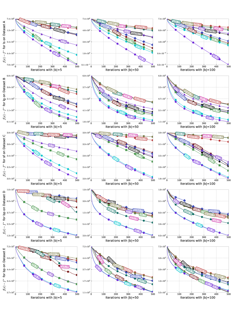
Figure 8: Comparison of different random and greedy block selection rules on five different problems (rows) with three different blocks (columns) when using gradient updates.

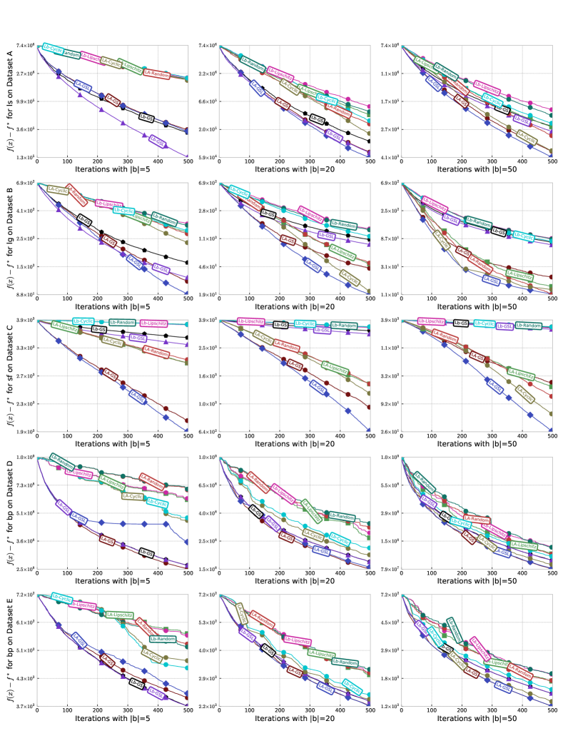
Figure 9: Comparison of different random and greedy block selection rules with gradient updates and fixed blocks, using two different strategies to estimate $L_{b}$.

In Figure 8 we show the performance of the different methods from Section 7.1 on all five datasets with three different block sizes. In Figure 9 we repeat the experiment but focusing only on the FB methods that do not incorporate the Lipschitz constant. For each FB method, we plot the performance using our upper bounds on $L_{b}$ as the step-size (Lb) and using the Lipschitz approximation procedure from Section 4.3 (LA). Here we see the LA methods improves performance when using large block sizes and in cases where the global $L_{b}$ bound is not tight. Interestingly, the cyclic and random methods seem to perform as well as greedy when using LA and a large block size (we expect this would only be true for FB).

Our third experiment also focused on the FB methods, but considered different ways to partition the variables into fixed blocks. We considered three approaches:

1. Order: we partition the variables based on their numerical order (which is similar to using a random order for dataset except Dataset D, where this method groups variables that adjacent in the lattice).

2. Avg: we compute the coordinate-wise Lipschitz constants $L_{i}$, and place the largest $L_{i}$ with the smallest $L_{i}$ values so that the average $L_{i}$ values are similar across the blocks.

3. Sort: we sort the $L_{i}$ values and place the largest values together (and the smallest values together).

We compared many variations on cyclic/random/greedy rules with gradient or matrix updates. In the case of greedy rules with gradient updates, we found that the Sort method tended to perform the best while the Order method tended to perform the worst (see Figure 10). When using matrix updates or when using cyclic/randomized rules, we found that no partitioning strategy dominated other strategies.

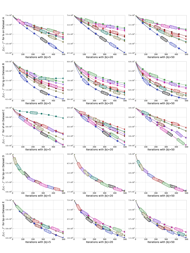
Figure 10: Comparison of different random and greedy block selection rules with gradient updates and fixed blocks, using three different ways to partition the variables into blocks.

Appendix F.3 Greedy Rules with Matrix and Newton Updates

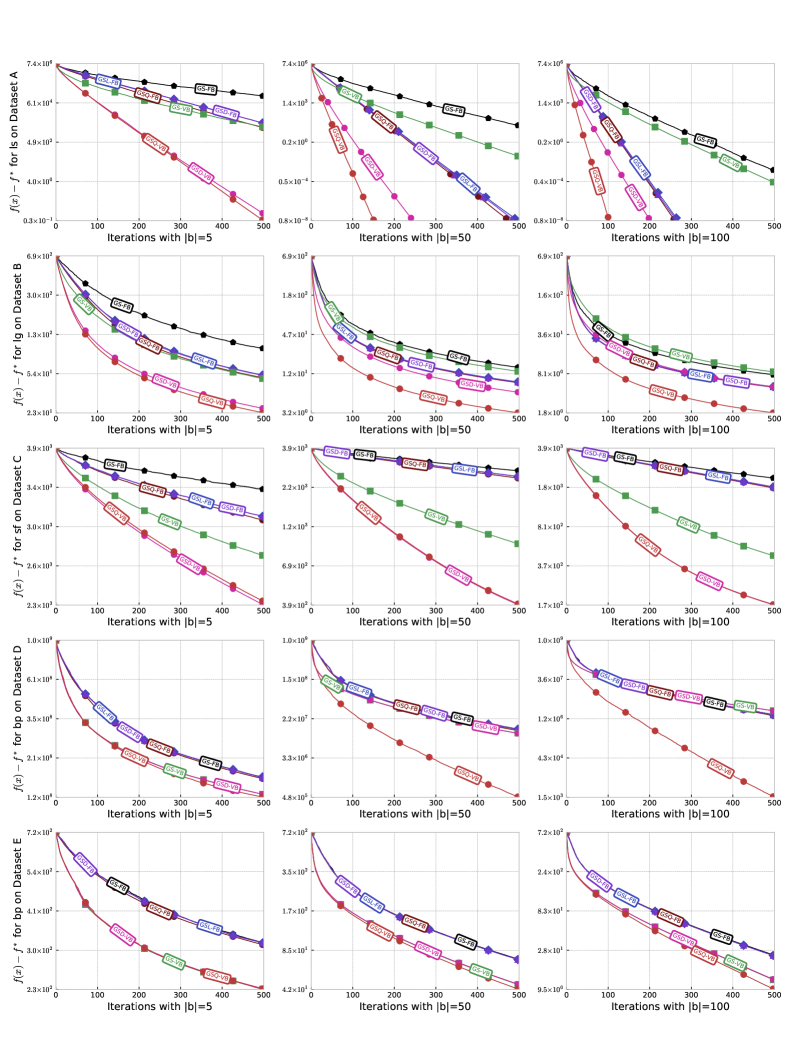
Figure 11: Comparison of different greedy block selection rules when using matrix updates.

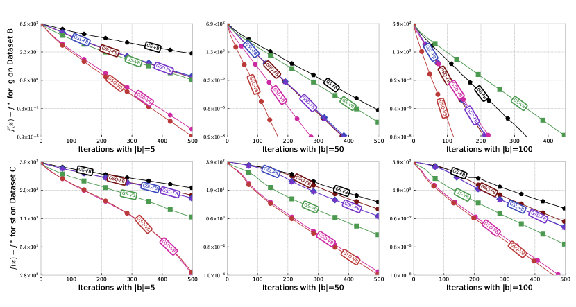
Figure 12: Comparison of different greedy block selection rules when using Newton updates and a line-search.

In Figure 11 we show the performance of the different methods from Section 7.2 on all five datasets with three different block sizes. In Figure 12 we repeat this experiment on the two non-quadratic problems, using the Newton direction and a line-search rather than matrix updates. We see that using Newton’s method significantly improves performance over matrix updates.

Appendix F.4 Proximal Updates using Random Selection

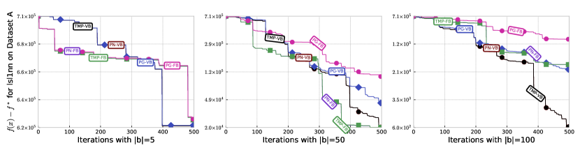
Figure 13: Comparison of different updates when using random fixed and variable blocks of different sizes on a non-smooth problem.

In Figure 7 we compare the performance of a projected gradient update with $L_{b}$ step-size, a projected Newton (PN) solver with line-search and the two-metric projection (TMP) update when using greedy selected fixed (FB) and variable (VB) blocks of different sizes ($|b|={5,50,100}$). In Figure 13 we repeat this experiment using randomly selected blocks. We see that for such a sparse problem the random block selection rules suffer from selecting variables that are already zero/active, as seen by the step-like nature of the results.

References

- Amaral et al. (2022) V. Amaral, R. Andreani, E. Birgin, D. Marcondes, and J. Martínez. On complexity and convergence of high-order coordinate descent algorithms for smooth nonconvex box-constrained minimization. Journal of Global Optimization, pages 1–35, 2022.
- Baghel et al. (2013) M. Baghel, S. Agrawal, and S. Silakari. Recent trends and developments in graph coloring. International Conference on Frontiers of Intelligent Computing: Theory and Applications, 2013.
- Bakin (1999) S. Bakin. Adaptive regression and model selection in data mining problems. PhD thesis, Australian National University, Canberra, Australia, 1999.
- Beck and Tetruashvili (2013) A. Beck and L. Tetruashvili. On the convergence of block coordinate descent type methods. SIAM J. Optim., 23(4):2037–2060, 2013.
- Bertsekas (1976) D. P. Bertsekas. On the Goldstein-Levitin-Polyak gradient projection method. IEEE Transactions on Automatic Control, 21(2):174–184, 1976.
- Bertsekas (2016) D. P. Bertsekas. Nonlinear Programming. Athena Scientific, 3rd edition, 2016.
- Bickson (2009) D. Bickson. Gaussian Belief Propagation: Theory and Application. PhD thesis, The Hebrew University of Jerusalem, Jerusalem, Israel, 2009.
- Blumensath and Davies (2009) T. Blumensath and M. E. Davies. Iterative hard thresholding for compressed sensing. Appl. Comput. Harmon. Anal., 27(3):265–274, 2009.
- Bo and Sminchisescu (2008) L. Bo and C. Sminchisescu. Greedy block coordinate descent for large scale gaussian process regression. Conference on Uncertainty in Artificial Intelligence, 2008.
- Böhning (1992) D. Böhning. Multinomial logistic regression algorithm. Ann. Inst. Stat. Math., 44(1):197–200, 1992.
- Boyd and Vandenberghe (2004) S. Boyd and L. Vandenberghe. Convex Optimization. Cambridge University Press, 2004.
- Burke and Moré (1988) J. V. Burke and J. J. Moré. On the identification of active constraints. SIAM J. Numer. Anal., 25(5):1197–1211, 1988.
- Chang and Lin (2011) C.-C. Chang and C.-J. Lin. LIBSVM: A library for support vector machines. ACM Trans. Intell. Syst. Technol., 2(3):27:1–27:27, 2011.
- Chen et al. (2012) B. Chen, S. He, Z. Li, and S. Zhang. Maximum block improvement and polynomial optimization. SIAM J. Optim., 22(1):87–107, 2012.
- Csiba and Richtárik (2017) D. Csiba and P. Richtárik. Global convergence of arbitrary-block gradient methods for generalized Polyak-ojasiewicz functions. arXiv:1709.03014, 2017.
- Csiba and Richtárik (2018) D. Csiba and P. Richtárik. Importance sampling for minibatches. The Journal of Machine Learning Research, 19(1):962–982, 2018.
- Csiba et al. (2015) D. Csiba, Z. Qu, and P. Richtárik. Stochastic dual coordinate ascent with adaptive probabilities. International Conference on Machine Learning, 2015.
- Dahl et al. (2008) J. Dahl, L. Vandenberghe, and V. Roychowdhury. Covariance selection for nonchordal graphs via chordal embedding. Optim. Methods Softw., 23(4):501–520, 2008.
- De Santis et al. (2016) M. De Santis, S. Lucidi, and F. Rinaldi. A fast active set block coordinate descent algorithm for -regularized least squares. SIAM J. Optim., 26(1):781–809, 2016.
- Dembo et al. (1982) R. S. Dembo, S. C. Eisenstat, and T. Steihaug. Inexact Newton methods. SIAM J. Numer. Anal., 19(2):400–408, 1982.
- Dennis and Moré (1974) J. E. Dennis and J. J. Moré. A characterization of superlinear convergence and its application to quasi-Newton methods. Math. Comput., 28(126):549–560, 1974.
- Dhillon et al. (2011) I. S. Dhillon, P. K. Ravikumar, and A. Tewari. Nearest neighbor based greedy coordinate descent. Advances in Neural Information Processing Systems, 2011.
- Efron et al. (2004) B. Efron, T. Hastie, I. Johnstone, and R. Tibshirani. Least angle regression. Ann. Stat., 32(2):407–451, 2004.
- Ene and Nguyen (2015) A. Ene and H. L. Nguyen. Random coordinate descent methods for minimizing decomposable submodular functions. International Conference on Machine Learning, 2015.
- Esperet et al. (2015) L. Esperet, L. Lemoine, and F. Maffray. Equitable partition of graphs into induced forests. Discrete Math., 338:1481–1483, 2015.
- Fang et al. (2020) H. Fang, Z. Fan, Y. Sun, and M. Friedlander. Greed meets sparsity: Understanding and improving greedy coordinate descent for sparse optimization. International Conference on Artificial Intelligence and Statistics, 2020.
- Fang et al. (2021) H. Fang, G. Fang, T. Yu, and P. Li. Efficient greedy coordinate descent via variable partitioning. Uncertainty in Artificial Intelligence, 2021.
- Fercoq and Richtárik (2015) O. Fercoq and P. Richtárik. Accelerated, parallel and proximal coordinate descent. SIAM J. Optim., 25(4):1997–2023, 2015.
- Fountoulakis and Tappenden (2018) K. Fountoulakis and R. Tappenden. A flexible coordinate descent method. Computational Optimization and Applications, 70(2):351–394, 2018.
- Fountoulakis et al. (2016) K. Fountoulakis, F. Roosta-Khorasani, J. Shun, X. Cheng, and M. W. Mahoney. Exploiting optimization for local graph clustering. arXiv:1602.01886, 2016.
- Fu (1998) W. J. Fu. Penalized regressions: the bridge versus the lasso. J. Comput. Graph. Stat., 7(3):397–416, 1998.
- Gafni and Bertsekas (1984) E. M. Gafni and D. P. Bertsekas. Two-metric projection methods for constrained optimization. SIAM J. Control Optim., 22(6):936–964, 1984.
- Garey and Johnson (1979) M. R. Garey and D. S. Johnson. Computers and Intractability: A Guide to the Theory of NP-Completeness. W. H. Freeman & Co., New York, USA, 1979.
- Glasmachers and Dogan (2013) T. Glasmachers and U. Dogan. Accelerated coordinate descent with adaptive coordinate frequencies. Asian Conference on Machine Learning, 2013.
- Gregor and Fessler (2015) J. Gregor and J. A. Fessler. Comparison of SIRT and SQS for regularized weighted least squares image reconstruction. IEEE Trans. Comput. Imaging, 1(1):44–55, 2015.
- Hare (2011) W. L. Hare. Identifying active manifolds in regularization problems. In H. H. Bauschke, R. S. Burachik, P. L. Combettes, V. Elser, D. R. Luke, and H. Wolkowicz, editors, Fixed-Point Algorithms for Inverse Problems in Science and Engineering, pages 261–271. Springer New York, New York, NY, 2011.
- Hare and Lewis (2004) W. L. Hare and A. S. Lewis. Identifying active constraints via partial smoothness and prox-regularity. J. Convex Analysis, 11(2):251–266, 2004.
- Harrar (1993) D. L. Harrar. Orderings, multicoloring, and consistently ordered matrices. SIAM J. Matrix Anal. Appl., 14(1):259–278, 1993.
- Hastie et al. (2004) T. Hastie, S. Rosset, R. Tibshirani, and J. Zhu. The entire regularization path for the support vector machine. J. Mach. Learn. Res., 5:1391–1415, 2004.
- Hocking (1976) R. R. Hocking. A biometrics invited paper. The analysis and selection of variables in linear regression. Biometrics, 32(1):1–49, 1976.
- Horn et al. (2018) D. Horn, A. Demircioğlu, B. Bischl, T. Glasmachers, and C. Weihs. A comparative study on large scale kernelized support vector machines. Adv. Data Anal. Classi., 12(4):867–883, 2018.
- Hsieh et al. (2013) C.-J. Hsieh, M. A. Sustik, I. S. Dhillon, P. Ravikumar, and R. Poldrack. BIG & QUIC: Sparse inverse covariance estimation for a million variables. Advances in Neural Information Processing Systems, 2013.
- Jegelka et al. (2013) S. Jegelka, F. Bach, and S. Sra. Reflection methods for user-friendly submodular optimization. Advances in Neural Information Processing Systems, 2013.
- Joachims (1999) T. Joachims. Making large-scale SVM learning practical. In B. Schölkopf, C. J. C. Burges, and A. J. Smola, editors, Advances in Kernel Methods - Support Vector Learning, pages 169–184. MIT Press, 1999.
- Karimi et al. (2016) H. Karimi, J. Nutini, and M. Schmidt. Linear convergence of gradient and proximal-gradient methods under the Polyak-ojasiewicz condition. European Conference on Machine Learning, 2016.
- Karimireddy et al. (2019) S. P. Karimireddy, A. Koloskova, S. U. Stich, and M. Jaggi. Efficient greedy coordinate descent for composite problems. International Conference on Artificial Intelligence and Statistics, 2019.
- Khan (2012) M. E. Khan. Variational Learning for Latent Gaussian Model of Discrete Data. PhD thesis, The University of British Columbia, Vancouver, Canada, 2012.
- Kyng and Sachdeva (2016) R. Kyng and S. Sachdeva. Approximate Gaussian elimination for Laplacians - fast, sparse, and simple. Foundations of Computer Science, 2016.
- Lee and Wright (2019) C.-P. Lee and S. J. Wright. Random permutations fix a worst case for cyclic coordinate descent. IMA Journal of Numerical Analysis, 39(3):1246–1275, 2019.
- Lee et al. (2012) J. D. Lee, Y. Sun, and M. A. Saunders. Proximal Newton-type methods for convex optimization. Advances in Neural Information Processing Systems, 2012.
- Lee and Wright (2012) S. Lee and S. J. Wright. Manifold identification in dual averaging for regularized stochastic online learning. J. Mach. Learn. Res., 13(Jun):1705–1744, 2012.
- Lei et al. (2016) Q. Lei, K. Zhong, and I. S. Dhillon. Coordinate-wise power method. Advances in Neural Information Processing Systems, 2016.
- Li et al. (2015) Z. Li, A. Uschmajew, and S. Zhang. On convergence of the maximum block improvement method. SIAM J. Optim., 25(1):210–233, 2015.
- Liang et al. (2017) J. Liang, J. Fadili, and G. Peyré. Activity identification and local linear convergence of forward–backward-type methods. SIAM J. Optim., 27(1):408–437, 2017.
- Locatello et al. (2018) F. Locatello, A. Raj, S. P. Karimireddy, G. Rätsch, B. Schölkopf, S. U. Stich, and M. Jaggi. On matching pursuit and coordinate descent. International Conference on Machine Learning, 2018.
- Lopes et al. (2019) R. Lopes, S. A. Santos, and P. J. S. Silva. Accelerating block coordinate descent methods with identification strategies. Comput. Optim. Appl., 72(3):609–640, 2019.
- Lu et al. (2018) H. Lu, R. M. Freund, and V. Mirrokni. Accelerating greedy coordinate descent methods. International Conference on Machine Learning, 2018.
- Mairal and Yu (2012) J. Mairal and B. Yu. Complexity analysis of the lasso regularization path. International Conference on Machine Learning, 2012.
- Malioutov et al. (2006) D. M. Malioutov, J. K. Johnson, and A. S. Willsky. Walk-sums and belief propagation in Gaussian graphical models. J. Mach. Learn. Res., 7(Oct):2031–2064, 2006.
- Megiddo (1979) N. Megiddo. Combinatorial optimization with rational objective functions. Math. Oper. Res., 4(4):414–424, 1979.
- Meier et al. (2008) L. Meier, S. Van De Geer, and P. Bühlmann. The group lasso for logistic regression. J. R. Stat. Soc. Series B Stat. Methodol., 70(1):53–71, 2008.
- Meshi et al. (2012) O. Meshi, T. Jaakkola, and A. Globerson. Convergence rate analysis of MAP coordinate minimization algorithms. Advances in Neural Information Processing Systems, 2012.
- Mifflin and Sagastizábal (2002) R. Mifflin and C. Sagastizábal. Proximal points are on the fast track. J. Convex Anal., 9(2):563–579, 2002.
- Mutny et al. (2020) M. Mutny, M. Derezinski, and A. Krause. Convergence analysis of block coordinate algorithms with determinantal sampling. International Conference on Artificial Intelligence and Statistics, 2020.
- Namkoong et al. (2017) H. Namkoong, A. Sinha, S. Yadlowsky, and J. C. Duchi. Adaptive sampling probabilities for non-smooth optimization. International Conference on Machine Learning, 2017.
- Needell and Tropp (2014) D. Needell and J. A. Tropp. Paved with good intentions: Analysis of a randomized block Kaczmarz method. Linear Algebra Appl., 441:199–221, 2014.
- Nesterov (2004) Y. Nesterov. Introductory Lectures on Convex Optimization: A Basic Course. Kluwer Academic Publishers, Dordrecht, The Netherlands, 2004.
- Nesterov (2012) Y. Nesterov. Efficiency of coordinate descent methods on huge-scale optimization problems. SIAM J. Optim., 22(2):341–362, 2012.
- Nesterov and Polyak (2006) Y. Nesterov and B. T. Polyak. Cubic regularization of Newton method and its global performance. Math. Program., pages 177–205, 2006.
- Nocedal and Wright (1999) J. Nocedal and S. J. Wright. Numerical Optimization. Springer, 1999.
- Nutini et al. (2015) J. Nutini, M. Schmidt, I. H. Laradji, M. Friedlander, and H. Koepke. Coordinate descent converges faster with the Gauss-Southwell rule than random selection. International Conference on Machine Learning, 2015.
- Nutini et al. (2019) J. Nutini, M. Schmidt, and W. Hare. “Active-set complexity” of proximal gradient: How long does it take to find the sparsity pattern? Optim. Lett., 13(4):645–655, 2019.
- Ortega and Rheinboldt (1970) J. M. Ortega and W. C. Rheinboldt. Iterative Solution of Nonlinear Equations in Several Variables. New York: Acedemic Press, 1970.
- Osborne and Turlach (2011) M. R. Osborne and B. A. Turlach. A homotopy algorithm for the quantile regression lasso and related piecewise linear problems. J. Comput. Graph. Stat., 20(4):972–987, 2011.
- Osborne et al. (2000) M. R. Osborne, B. Presnell, and B. A. Turlach. A new approach to variable selection in least squares problems. IMA J. Numer. Anal., 20(3):389–403, 2000.
- Parter (1961) S. Parter. The use of linear graphs in Gauss elimination. SIAM Rev., 3(2):119–130, 1961.
- Pati et al. (1993) Y. C. Pati, R. Rezaiifar, and P. S. Krishnaprasad. Orthogonal matching pursuit: Recursive function approximation with applications to wavelet decomposition. In Proceedings of the 27th Annual Asilomar Conference Signals, Systems and Computers, pages 40–44. IEEE, 1993.
- Perekrestenko et al. (2017) D. Perekrestenko, V. Cevher, and M. Jaggi. Faster coordinate descent via adaptive importance sampling. International Conference on Artificial Intelligence and Statistics, 2017.
- Pilanci and Wainwright (2017) M. Pilanci and M. J. Wainwright. Newton sketch: A linear-time optimization algorithm with linear-quadratic convergence. SIAM J. Optim., 27(1):205–245, 2017.
- Platt (1998) J. C. Platt. Sequential minimal optimization: A fast algorithm for training support vector machines. Technical report, Microsoft Research, 1998.
- Polyak (1963) B. T. Polyak. Gradient methods for minimizing functionals (in Russian). Zh. Vychisl. Mat. Mat. Fiz., pages 643–653, 1963.
- Qin et al. (2013) Z. Qin, K. Scheinberg, and D. Goldfarb. Efficient block-coordinate descent algorithms for Group Lasso. Mathematical Programming Computation, 5:143–169, 2013.
- Qu and Richtárik (2016) Z. Qu and P. Richtárik. Coordinate descent with arbitrary sampling I: Algorithms and complexity. Optim. Methods Softw., 31(5):829–857, 2016.
- Qu and Richtárik (2016) Z. Qu and P. Richtárik. Coordinate descent with arbitrary sampling II: Expected separable overapproximation. Optim. Methods Softw., 31(5):858–884, 2016.
- Qu et al. (2015) Z. Qu, P. Richtárik, and T. Zhang. Randomized dual coordinate ascent with arbitrary sampling. Advances in Neural Information Processing Systems, 2015.
- Qu et al. (2016) Z. Qu, P. Richtárik, M. Takáč, and O. Fercoq. SDNA: Stochastic dual coordinate ascent for empirical risk minimization. International Conference on Machine Learning, 2016.
- Richtárik and Takáč (2016) P. Richtárik and M. Takáč. Parallel coordinate descent methods for big data optimization. Math. Prog., 156(1-2):433–484, 2016.
- Richtárik and Takáč (2014) P. Richtárik and M. Takáč. Iteration complexity of randomized block-coordinate descent methods for minimizing a composite function. Math. Program., 144:1–38, 2014.
- Richtárik and Takáč (2016) P. Richtárik and M. Takáč. On optimal probabilities in stochastic coordinate descent methods. Optimization Letters, 10(6):1233–1243, 2016.
- Rockafellar (1976) R. T. Rockafellar. Monotone operators and the proximal point algorithm. SIAM J. Control Optim., 14(5):877–898, 1976.
- Rodomanov and Kropotov (2020) A. Rodomanov and D. Kropotov. A randomized coordinate descent method with volume sampling. SIAM Journal on Optimization, 30(3):1878–1904, 2020.
- Rose (1970) D. J. Rose. Triangulated graphs and the elimination process. J. Math. Anal. Appl., 32(3):597–609, 1970.
- Rosset and Zhu (2007) S. Rosset and J. Zhu. Piecewise linear regularized solution paths. Ann. Stat., 35(3):1012–1030, 2007.
- Saad (2003) Y. Saad. Iterative Methods for Sparse Linear Systems. SIAM, 2003.
- Sardy et al. (2000) S. Sardy, A. G. Bruce, and P. Tseng. Block coordinate relaxation methods for nonparametric wavelet denoising. J. Comput. Graph. Stat., 9(2):361–379, 2000.
- Scheinberg and Rish (2009) K. Scheinberg and I. Rish. SINCO-a greedy coordinate ascent method for sparse inverse covariance selection problem. Optimization Online preprint, 2009.
- Scherrer et al. (2012) C. Scherrer, A. Tewari, M. Halappanavar, and D. J. Haglin. Feature clustering for accelerating parallel coordinate descent. Advances in Neural Information Processing Systems, 2012.
- Schmidt (2010) M. Schmidt. Graphical Model Structure Learning with -Regularization. PhD thesis, The University of British Columbia, Vancouver, Canada, 2010.
- Shental et al. (2008) O. Shental, P. H. Siegel, J. K. Wolf, D. Bickson, and D. Dolev. Gaussian belief propagation solver for systems of linear equations. In IEEE International Symposium on Information Theory, 2008.
- Song et al. (2017) C.-B. Song, S. Cui, Y. Jiang, and S.-T. Xia. Accelerated stochastic greedy coordinate descent by soft thresholding projection onto simplex. Advances in Neural Information Processing Systems, 2017.
- Sontag and Jaakkola (2009) D. Sontag and T. Jaakkola. Tree block coordinate descent for MAP in graphical models. In Proceedings of the 12th International Conference on Artificial Intelligence and Statistics, pages 544–551, Clearwater Beach, USA, 2009.
- Srinivasan and Todorov (2015) A. Srinivasan and E. Todorov. Graphical Newton. arXiv:1508.00952, 2015.
- Stich et al. (2017) S. U. Stich, A. Raj, and M. Jaggi. Approximate steepest coordinate descent. International Conference on Machine Learning, 2017.
- Sun et al. (2014) Y. Sun, M. S. Andersen, and L. Vandenberghe. Decomposition in conic optimization with partially separable structure. SIAM J. Optim., 24(2):873–897, 2014.
- Tappenden et al. (2016) R. Tappenden, P. Richtárik, and J. Gondzio. Inexact coordinate descent: Complexity and preconditioning. J. Optim. Theory Appl., pages 144–176, 2016.
- Thoppe et al. (2014) G. Thoppe, V. S. Borkar, and D. Garg. Greedy block coordinate descent (GBCD) method for high dimensional quadratic programs. arXiv:1404.6635, 2014.
- Tseng and Yun (2009a) P. Tseng and S. Yun. A coordinate gradient descent method for nonsmooth separable minimization. Math. Program., 117:387–423, 2009a.
- Tseng and Yun (2009b) P. Tseng and S. Yun. Block-coordinate gradient descent method for linearly constrained nonsmooth separable optimization. J. Optim. Theory Appl., pages 513–535, 2009b.
- Vandenberghe and Andersen (2015) L. Vandenberghe and M. S. Andersen. Chordal graphs and semidefinite optimization. Found. Trends Optim., 1(4):241–433, 2015.
- Welsh and Powell (1967) D. J. A. Welsh and M. B. Powell. An upper bound for the chromatic number of a graph and its application to timetabling problems. The Computer Journal, 10(1):85–86, 1967.
- Wright (1993) S. J. Wright. Identifiable surfaces in constrained optimization. SIAM J. Control Optim., 31(4):1063–1079, 1993.
- Wright (2012) S. J. Wright. Accelerated block-coordinate relaxation for regularized optimization. SIAM J. Optim., 22(1):159–186, 2012.
- Xu and Yin (2013) Y. Xu and W. Yin. A block coordinate descent method for regularized multiconvex optimization with applications to nonnegative tensor factorization and completion. SIAM J. Imaging Sci, 6(3):1758–1789, 2013.
- You et al. (2016) Y. You, X. Lian, J. Liu, H.-F. Yu, I. S. Dhillon, J. Demmel, and C.-J. Hsieh. Asynchronous parallel greedy coordinate descent. Advances in Neural Information Processing Systems, 2016.
- Young (1971) D. M. Young. Iterative Solution of Large Linear Systems. New York: Academic Press, 1971.
- Yu et al. (2012) H.-F. Yu, C.-J. Hsieh, S. Si, and I. S. Dhillon. Scalable coordinate descent approaches to parallel matrix factorization for recommender systems. International Conference on Data Mining, 2012.
- Zhou et al. (2003) D. Zhou, O. Bousquet, T. N. Lal, J. Weston, and B. Schölkopf. Learning with local and global consistency. Advances in Neural Information Processing Systems, 2003.