Abstract: This paper solves the two-dimensional Dirichlet problem for the Monge-Ampère equation by a strong meshless collocation technique that uses a polynomial trial space and collocation in the domain and on the boundary. Convergence rates may be up to exponential, depending on the smoothness of the true solution, and this is demonstrated numerically and proven theoretically, applying a sufficiently fine collocation discretization. A much more thorough investigation of meshless methods for fully nonlinear problems is in preparation.
 

AMS Classification: 35J36, 65D99, 65N12, 65N35
 

Keywords: Collocation, fully nonlinear PDE, Monge–Ampère, nonlinear optimizer, MATLAB implementation, convergence, error analysis, error estimates.

1 Introduction

The Dirichlet problem for the Monge-Ampère equation on a bounded domain ${\Omega}\subset\mathbb{R}^{d}$ consists in finding a smooth function $u$ on $\overline{\Omega}$ such that the equations

$$\begin{array}[]{rcl}u_{xx}u_{yy}-u_{xy}^{2}&=&g\hbox{ in }\overline{\Omega}\\ u&=&f\hbox{ in }\partial\Omega\end{array}$$ (1)

hold, where the functions $f$ and $g$ are given on the boundary $\partial\Omega$ and on $\overline{\Omega}$, respectively. The goal of this contribution is to show how simply meshless methods in strong form can be applied and their convergence be proven for this most important special case of a fully nonlinear second-order partial differential equation, thoroughly investigated in Böhmer/Schaback [5]. Concerning simplicity, the meshless method proposed here is strongly superior to the complicated approaches for difference methods in Oberman [18] and finite elements. The first method including convergence is published in Böhmer [2], based upon smooth finite elements of Davydov and Saeed [8, 9]. See also Brenner et al. [7] and Feng/Neilan [11] for a method to solve the Monge-Ampère equations via finite elements and a $C^{0}$ penalty method or a vanishing moment method.

To explain the connection to the general situation, the equation is rewritten as

$$\begin{array}[]{rcll}Fu&=&g&\hbox{ in }\overline{\Omega}\\ u&=&f&\hbox{ in }\Gamma:=\partial\Omega\end{array}$$

with the nonlinear map $F\;:\;u\mapsto u_{xx}u_{yy}-u_{xy}^{2}$. which is defined as a mapping

$$F\;:\;C^{2}(\overline{\Omega})\to C(\overline{\Omega}).$$ (2)

Fully nonlinear problems are those where second-order derivatives arise nonlinearly in $F$. Existence and regularity results from the literature are collected in [3], Theorems 2.79-2.82.

Under appropriate assumptions, there is a unique solution $u^{*}\in C^{2}(\overline{\Omega})$. Then the connection to linear elliptic problems is made by the linearization at $u^{*}$, namely

$$F^{\prime}(u^{*})(v)=u^{*}_{xx}v_{yy}+v_{xx}u^{*}_{yy}-2u^{*}_{xy}v_{xy}.$$

By the cited background literature collected in [3], this $F^{\prime}(u^{*})$ defines an elliptic operator for a convex locally unique solution $u^{*}$. There also is a variation of a maximum principle, and $F^{\prime}(u^{*})$ is boundedly invertible.

2 Strong Meshfree Discretizations

These techniques discretize PDE problems using

1. a trial space that should approximate the true solution $u^{*}$ well, and

2. sets of test points on which the differential operator and the boundary conditions are directly sampled,

3. forming a nonlinear system of collocation equations that is possibly overdetermined, and finally

4. applying a nonlinear optimizer to minimize residuals of the system.

In contrast to finite element methods, there is no connection between the test and the trial side via a triangularization, and there is no numerical integration. Consistency is guaranteed by choosing a sufficiently rich trial space, and stability requires to choose sufficiently many well-posed collocation points. The details concerning these choices are nontrivial and will not be explained here, see e.g. [19, 4, 20] for a comprehensive convergence analysis.

To present a simple example that works for the Monge-Ampère equation, we confine the domain $\Omega$ to be the unit square $[-1,+1]^{2}$ and use polynomial trial functions

$$u^{C}(x,y):=\displaystyle{\sum_{m=0}^{M}\sum_{n=0}^{M-m}c_{mn}x^{m}y^{n}}$$ (3)

of total degree at most $M$ that will approximate smooth solutions well. The coefficients are collected into a triangular matrix $C$. Other parametrized trial spaces could serve the same purpose, but the trial functions should be smooth and derivatives up to second order should be available at low computational cost.

On the test side, we take $K_{D}$ points $z_{i}^{D}:=(x_{i}^{D},y_{i}^{D}),\;1\leq i\leq K_{D}$ in the closure of the domain for approximation of the differential operator, and additionally $K_{B}$ points $z_{i}^{B}:=(x_{i}^{B},y_{i}^{B}),\;1\leq i\leq K_{B}$ on the boundary, forming point sets $Z^{D}$ and $Z^{B}$. These sets may have a nonempty intersection on the boundary.

The strong meshless discretization then sets up a nonlinear system

$$\begin{array}[]{rcl}u^{C}_{xx}(z_{i}^{D})u^{C}_{yy}(z_{i}^{D})-u^{C}_{xy}(z_{i}^{D})^{2}&=&g(z_{i}^{D}),\;1\leq i\leq K_{D}\\ u^{C}(z_{j}^{B})&=&f(z_{j}^{B}),\;1\leq i\leq K_{B}\end{array}$$

for the coefficient matrix $C$. There is no linearization done here. Linearization is left to the solver.

Brute-force numerical methods can then apply either a nonlinear equation solver to the system or a nonlinear optimizer to the residuals. Because oversampling will often be necessary to guarantee stability [19, 4, 20], the latter situation is preferable. This paper uses the nonlinear least-squares minimizer nlsqnonlin of MATLAB on the residuals of the above nonlinear system. No matter how the nonlinear solver works, the possibility of multiple local solutions requires good initial startup parameters. If none are known from external arguments, a standard technique is to apply repeated calculations using larger and larger trial spaces, starting from the optimal solution of the previous step. In parallel, the test discretizations should be refined from step to step. See Fasshauer’s book [10] for a comprehensive account of meshless methods using MATLAB.

A similar meshless algorithm, but without a convergence analysis, and with different trial functions, was proposed by Zhiyong Liu and collaborators [16, 17, 14], based on Kansa’s unsymmetric collocation. Finite differences and multigrid methods were applied by various authors [1, 12, 13, 15], but these techniques are further away from this work because they are not meshless and much more difficult to implement.

Readers may jump to Section 4 for MATLAB implementation details, and to Section 5 for the theoretical error analysis. We shall present the numerical results next, and finally add a summary and an outlook.

3 Numerical Results

The example of this paper uses the true solution

$$u^{*}(x,y)=\exp((x^{2}+y^{2})/2)$$ (4)

to generate the appropriate functions $f$ and $g$ in (1).

If the truncated Taylor expansion of the true solution is used as a starting approximation, Figure 1 shows the exponential decay of the error as a function of the total degree $M$ in (3).

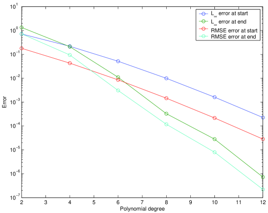
Figure 1: Errors as functions of degree

Here, RMSE stands for the root-mean-square error. If we start with the constant approximation 1 at degree zero and use the best coefficients for degree $M$ to start at degree $M+2$, we get Figure 2.

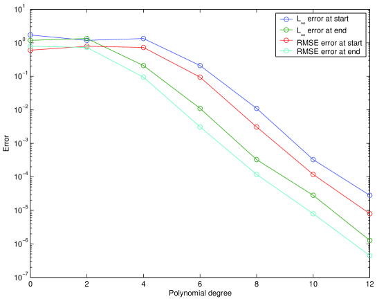
Figure 2: Errors as functions of degree

We add figures for the final $M=12$ calculation, starting from the optimal $M=10$ result.

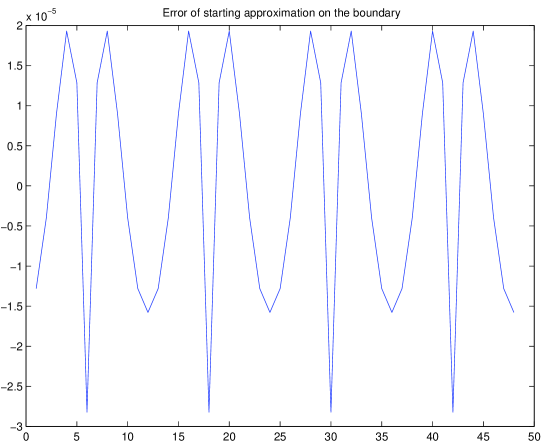
Figure 3: Starting error on the boundary

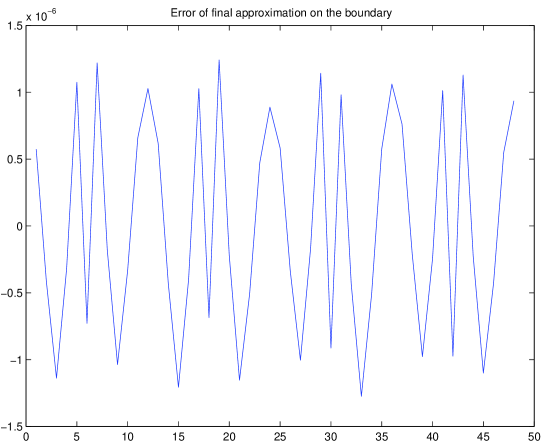
Figure 4: Final error on the boundary

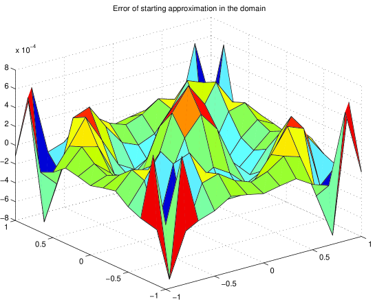
Figure 5: Starting error in the PDE

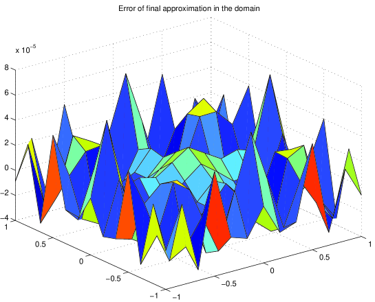
Figure 6: Final error in the PDE

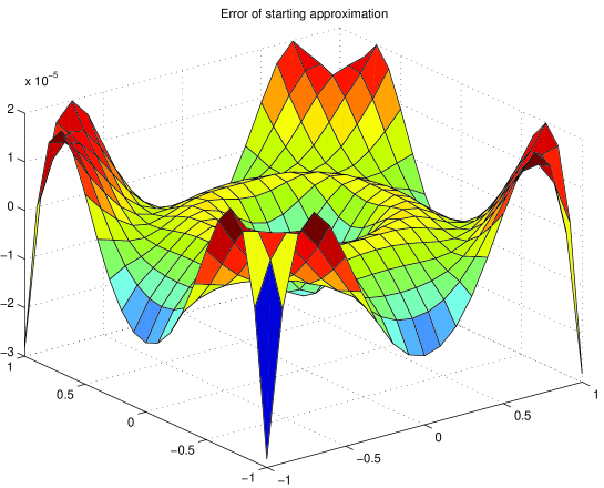
Figure 7: Starting error wrt. the solution

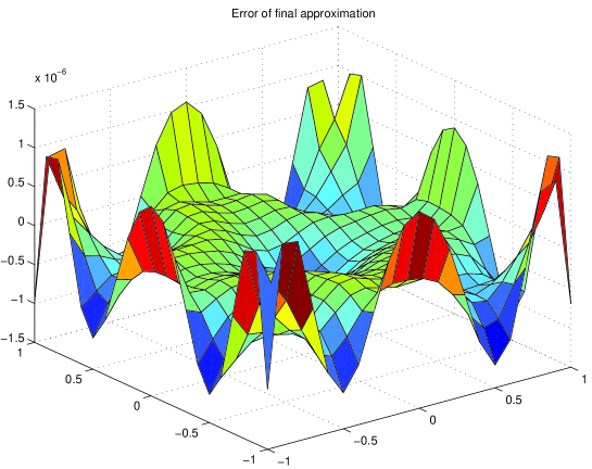
Figure 8: Final error wrt. the solution

The results are rather promising and justify a more general analysis to be provided in [5].

4 MATLAB Implementation Details

The unknown coefficients are stored in a triangular matrix $C$. At each point $p_{i}=(x_{i},y_{i})$ we pre–calculate the triangular Vandermonde matrix $Pu_{i}$ with entries $x_{i}^{m}\cdot y_{i}^{n}$ for $0\leq m+n\leq M$. Since the coefficient matrix $C$ has the same shape, we can take the elementwise product of $C$ and $Pu_{i}$, i.e. we form $C.*Pu_{i}$ in MATLAB notation. Applying the sum function of MATLAB then yields $\hbox{\tt sum}(\hbox{\tt sum}(C.*Pu_{i}))=u^{C}(x_{i},y_{i})$. If $(x_{i},y_{i})$ is a boundary point, we form

$$f_{i}(C):=f(x_{i},y_{i})-u^{C}(x_{i},y_{i})=f(x_{i},y_{i})-\hbox{\tt sum}(\hbox{\tt sum}(C.*Pu_{i}))$$

and add $f_{i}(C)^{2}$ later into the minimization via the MATLAB function nsqnonlin. This cares for boundary value discretization.

For PDE discretization, we work similarly. In particular, the second derivatives

$$\begin{array}[]{rcl}u_{xx}(x,y)&=&\displaystyle{\sum_{m=2}^{M}\sum_{n=0}^{M-m}c_{mn}m(m-1)x^{m-2}y^{n}},\\ u_{xy}(x,y)&=&\displaystyle{\sum_{m=1}^{M}\sum_{n=1}^{M-m}c_{mn}mnx^{m-1}y^{n-1}},\\ u_{yy}(x,y)&=&\displaystyle{\sum_{m=0}^{M}\sum_{n=2}^{M-m}c_{mn}n(n-1)x^{m}y^{n-2}}\\ \end{array}$$

are assembled at each point $(x_{i},y_{i})$ into triangular matrices $P_{xx}u_{i},\,P_{xy}u_{i},\,P_{yy}u_{i}$ with the above entries, and we get

$$\begin{array}[]{rcl}u_{xx}(x_{i},y_{i})(C)&=&\hbox{\tt sum}(\hbox{\tt sum}(C.*P_{xx}u_{i})),\\ u_{xy}(x_{i},y_{i})(C)&=&\hbox{\tt sum}(\hbox{\tt sum}(C.*P_{xy}u_{i})),\\ u_{yy}(x_{i},y_{i})(C)&=&\hbox{\tt sum}(\hbox{\tt sum}(C.*P_{yy}u_{i}))\\ \end{array}$$

as matrix-valued functions of the coefficient matrix $C$. If $(x_{i},y_{i})$ is a point where we want the discretized PDE to be satisfied, we define

$$\begin{array}[]{rcl}f_{i}(C)&:=&u_{xx}^{C}(x_{i},y_{i})u_{yy}^{C}(x_{i},y_{i})-u_{xy}^{C}(x_{i},y_{i})^{2}-g(x_{i},y_{i})\\ &=&\hbox{\tt sum}(\hbox{\tt sum}(C.*P_{xx}u_{i})).*\hbox{\tt sum}(\hbox{\tt sum}(C.*P_{yy}u_{i}))\\ &&-(\hbox{\tt sum}(\hbox{\tt sum}(C.*P_{xy}u_{i}))).{{}^{\wedge}}2-g(x_{i},y_{i})\end{array}$$

and add $f_{i}(C)^{2}$ into the minimization via nsqnonlin. This cares for the collocation of the nonlinear differential equation.

The total optimization problem then minimizes the sum of all these $f_{i}(C)^{2}$ with respect to the coefficient matrix $C$, using nlsqnonlin of MATLAB.

An additional simplification turned triangular matrices into vectors. Furthermore, the spatial discretization was changed with the polynomial degree. For $M>0$ we used regular data with spacing $h=2/M$, with $h=1$ for $M=0$. Choosing finer spatial discretizations does not improve the results. To give boundary values more weight, we multiplied the boundary $f_{i}(C)$ with 10 throughout.

5 Error Analysis

Since the paper [4] reduces the convergence analysis to the linearized strongly elliptic problem under the above circumstances, we only need to deal with the trial functions (3) used for solving a standard elliptic problem. Provided that sufficiently large sets of test points are chosen for each $M$, the paper [20] shows that the convergence rate is the one that arises when approximating the strong data of the solution, i.e. the second derivatives of the solution by such polynomials. Thus the convergence rate for the special case (4) is exponential, as can be either taken from Bernstein-type theorems in Approximation Theory or directly proven via the exponentially convergent Taylor expansion. The numerical results of Section 3 confirm this.

It is much more difficult to assess how many test points are sufficient for uniform stability. Considering Theorem 5.1 and (5.3) of [20], it suffices to prove conditions on the points that allow to bound $\|u^{C}\|_{\infty}$ uniformly in terms of the maximum or sum of the three discrete seminorms

$$\begin{array}[]{rcl}\|u^{C}\|_{0}&:=&\displaystyle{\max_{z_{i}^{B}\in Z^{B}}|u^{C}(z_{i}^{B})|}\\ \|u^{C}\|_{xx}&:=&\displaystyle{\max_{z_{i}^{D}\in Z^{D}}|u^{C}_{xx}(z_{i}^{D})|}\\ \|u^{C}\|_{yy}&:=&\displaystyle{\max_{z_{i}^{D}\in Z^{D}}|u^{C}_{yy}(z_{i}^{D})|}\\ \end{array}$$

for arbitrary trial functions $u^{C}$ of the form (3). Note that this is independent of PDEs. It is a problem of Approximation Theory. We can ignore the mixed derivatives and the factors depending on $u^{*}$ here, because uniform strong ellipticity allows to go over to the pure second derivatives, at the expense of uniformly bounded factors depending on $u^{*}$.

Using the standard machinery for proofs of stability inequalities, as nicely summarized in Chapter 3 of [21], we start with fill distances $h_{B}$ and $h_{D}$ for the points on the boundary and the domain, respectively, and deal with the boundary first. As a warm-up, consider the upper and lower boundary lines, i.e. two lines of length 2 parallel to the $x$ axis. There, each $u^{C}$ is a univariate polynomial $p$ of degree at most $M$, and we rewrite it as one on $[-1,+1]$. Now we know by Markov’s inequality that

$$\|p^{\prime}\|_{\infty,[-1,+1]}\leq M^{2}\|p\|_{\infty,[-1,+1]}.$$

For each point $x$ on the boundary lines there is a sample point $x_{i}$ at distance at most $h_{B}$, and thus

$$|p(x)|\leq|p(x_{i})|+h_{B}M^{2}\|p\|_{\infty,[-1,+1]}$$

proving $\|p\|_{\infty}\leq 2\max_{x_{i}}|p(x_{i})|$ on those boundary lines, if we have $h_{B}M^{2}\leq 1/2$. This proves

$$\|u^{C}\|_{\infty,\Gamma}\leq 2\max_{z_{i}^{B}\in Z_{B}}|u^{C}(z_{i}^{B})|$$

as soon as

$$h_{B}\leq\frac{1}{2}M^{-2}.$$

Note that Approximation Theory tells us that we can replace the exponent two by one, if ${\cal O}(M)$ points on the boundary are distributed in Chebyshev style.

The case with derivatives and interior points is not directly covered by the standard theory. From [6] we know that there is a well–posedness inequality

$$\|u\|_{\infty,\overline{\Omega}}\leq\|u\|_{\infty,\Gamma}+C\|\Delta u\|_{\infty,\overline{\Omega}}$$ (5)

for uniformly elliptic problems, and this can be applied to trial functions. We already have the first term on the right–hand side under control and only have to deal with the second term. Since all $\Delta u^{C}$ are polynomials as well as $u^{C}$, we can use the standard logic as in Chapter 3 of [21] to get a bound of the form

$$\|\Delta u^{C}\|_{\infty,\Omega}\leq 2\max_{z_{i}^{D}\in Z_{D}}|\Delta u^{C}(z_{i}^{D})|\leq 2\|u^{C}\|_{xx}+2\|u^{C}\|_{yy}$$

if $h_{D}\leq CM^{-2}$. Now the theory in [19, 4, 20] implies

Theorem 1

The strong meshless collocation method for solving the Monge-Ampère equation by trial functions (3) via sampling on test points with fill distances $h_{B}$ and $h_{D}$ on the boundary and the domain is uniformly stable if the fill distances behave like ${\cal O}(M^{-2})$. Furthermore, the convergence for $M\to\infty$ is exponential if the test points are chosen to guarantee uniform stability via sufficient oversampling. $\Box$

6 Summary and Outlook

By a specific example, it was demonstrated theoretically and numerically that a strong meshless discretization of the Monge-Ampère equation works successfully. This will generalize to subdomains of $[-1,+1]^{2}$ with Lipschitz boundaries on which bivariate polynomials are still polynomials. The domains should have a uniform interior cone condition.

Likewise, other trial spaces can be used. If the true solution is less smooth, convergence rates will then be confined to how well second derivatives of trial functions approximate second derivatives of the true solution. To guarantee stability for sufficient oversampling, the trial spaces must allow that the results of the previous section can be applied,

A much more thorough investigation of meshless methods for fully nonlinear problems is in preparation [5].

References

- [1] J.-D. Benamou, B.D. Froese, and A.M. Oberman. Two numerical methods for the elliptic Monge-Ampère equation. ESAIM: Mathematical Modelling and Numerical Analysis, 44(4):737–758, 2010.
- [2] K. Böhmer. On finite element methods for fully nonlinear elliptic equations of second order. SIAM J. Numer. Anal., 3:1212–1249, 2008.
- [3] K. Böhmer. Numerical Methods for Nonlinear Elliptic Differential Equations, a Synopsis. Oxford University Press, Oxford, 2010.
- [4] K. Böhmer and R. Schaback. A nonlinear discretization theory. Journal of Computational and Applied Mathematics, 254:204–219, 2013.
- [5] K. Böhmer and R. Schaback. Nonlinear discretization theory applied to meshfree methods and the Monge-Ampère equation. Fachbereich Mathematik und Informatik, Philipps–Universität Marburg, in preparation, 2016.
- [6] D. Braess. Finite Elements. Theory, Fast Solvers and Applications in Solid Mechanics. Cambridge University Press, 2001. Second edition.
- [7] S.C. Brenner, T. Gudi, M. Neilan, and L.Y. Sung. C0 penalty methods for the fully nonlinear Monge-Ampère equation. Mathematics of Computation, 80:1979 – 1995, 2011.
- [8] O. Davydov. Smooth finite elements and stable splitting. Fachbereich Mathematik und Informatik, Philipps–Universität Marburg, 2007.
- [9] O. Davydov and A. Saeed. Numerical solution of fully nonlinear elliptic equations by Böhmer’s method. J. Comp.Appl.Math., 254:43–54, 2013.
- [10] G. Fasshauer and M. McCourt. Kernel-based Approximation Methods using MATLAB, volume 19 of Interdisciplinary Mathematical Sciences. World Scientific, Singapore, 2015.
- [11] X. Feng and M. Neilan. Mixed finite element methods for the fully nonlinear Monge-Ampère equation based on the vanishing moment method. SIAM Journal on Numerical Analysis, 47:1226 – 1250, 2009.
- [12] B.D. Froese and A.M. Oberman. Convergent finite difference solvers for viscosity solutions of the elliptic Monge-Ampère equation in dimensions two and higher. SIAM Journal on Numerical Analysis, 49(4):1692–1714, 2011.
- [13] B.D. Froese and A.M. Oberman. Convergent filtered schemes for the Monge–Ampère partial differential equation. SIAM Journal on Numerical Analysis, 51(1):423–444, 2013.
- [14] Q. Li and Z.Y. Liu. Solving the 2-D elliptic Monge-Ampère equation by a Kansa’s method. Acta Mathematicae Applicatae Sinica, English Series, 33(2):269–276, Apr 2017.
- [15] J. Liu, B.D. Froese, A.M. Oberman, and M.Q. Xiao. A multigrid scheme for 3D Monge-Ampère equations. International Journal of Computer Mathematics, 94(9):1850–1866, 2017.
- [16] Z.Y. Liu and Y. He. Cascadic meshfree method for the elliptic Monge-Ampère equation. Engineering Analysis with Boundary Elements, 37(7):990 – 996, 2013.
- [17] Z.Y. Liu and Y. He. An iterative meshfree method for the elliptic Monge-Ampère equation in 2D. Numerical Methods for Partial Differential Equations, 30(5):1507–1517, 2014.
- [18] A. Oberman. Wide stencil finite difference schemes for the elliptic Monge-Ampère equations and functions of the eigenvalues of the Hessian. Discrete Contin. Dyn. Syst. Ser B 10(1), pages 221–238, 2008.
- [19] R. Schaback. Unsymmetric meshless methods for operator equations. Numerische Mathematik, 114:629–651, 2010.
- [20] R. Schaback. All well–posed problems have uniformly stable and convergent discretizations. Numerische Mathematik, 132:597–630, 2015.
- [21] H. Wendland. Scattered Data Approximation. Cambridge University Press, 2005.