Measuring the mass distribution in stellar systems

Abstract

One of the fundamental tasks of dynamical astronomy is to infer the distribution of mass in a stellar system from a snapshot of the positions and velocities of its stars. The usual approach to this task (e.g., Schwarzschild’s method) involves fitting parametrized forms of the gravitational potential and the phase-space distribution to the data. We review the practical and conceptual difficulties with this approach and describe a novel statistical method for determining the mass distribution that does not require determining the phase-space distribution of the stars. We show that this new estimator out-performs other distribution-free estimators for the harmonic and Kepler potentials.

1 Introduction

The determination of the mass distribution in stellar systems has led to some of the most important discoveries in astronomy. Examples include Kapteyn’s (1922) measurement of the local density in the Galactic disc; Zwicky’s (1933) discovery that the dark mass in the Coma cluster of galaxies is several hundred times larger than the mass in stars; measurements of the mass distribution in low-luminosity dwarf galaxies which show them also to be dominated by dark matter (e.g., Aaronson, 1983; McConnachie, 2012); and the determination of the mass of the central black hole in our Galaxy from the kinematics of the nuclear star cluster (e.g., Chakrabarty & Saha, 2001; Feldmeier-Krause et al., 2017). The scope and power of such measurements will grow in the near future, when the Gaia spacecraft provides accurate positions and velocities for $\sim 10^{9}$ stars in the Galaxy.

In this paper we examine an idealized formulation of this task. A set of $N$ test particles orbit in a gravitational potential $\Phi(\textbf{{x}}|\,\bm{\mu})$, where $\bm{\mu}=(\mu_{1},\mu_{2},\ldots)$ is a list of parameters that determine the analytic form of the potential. We call these mass parameters since the mass distribution follows directly from the potential via Poisson’s equation $\nabla^{2}\Phi=4\pi G\rho$. The system is assumed to be in a steady state, that is, the particles are distributed randomly in orbital phase. We know the positions and velocities of the particles at some instant, $\{\textbf{{x}}_{n},\textbf{{v}}_{n}\},$, $n=1,\ldots,N$. What can we infer about the mass parameters $\bm{\mu}$?

Perhaps the simplest astronomical example of this problem is to estimate the force law in the solar system from a snapshot of the positions and velocities of the eight planets. Bovy et al. (2010) use this example to motivate a wide-ranging discussion of the application of Bayesian methods to dynamical inference.

The idealized problem we examine here has only limited relevance to real astronomical systems, for several reasons. In most systems only two of the three spatial coordinates are known because the distance along the line of sight cannot be determined, and only one of the three velocity components is known because the proper motions are undetectably small. In addition, the survey region is often smaller than the system, so only a subset of the stars is measured. Finally, the measurement uncertainties in the velocities are often substantial. We shall not discuss these important practical issues, in order to focus on the simplest version of the task of mass determination, which is already complicated enough.

The test particles sample a distribution function (hereafter df) $F(\textbf{{x}},\textbf{{v}})$, defined such that $F(\textbf{{x}},\textbf{{v}})\,d\textbf{{x}}d\textbf{{v}}$ is the probability that a given particle is found in the small phase-space volume $d\textbf{{x}}d\textbf{{v}}$. Thus $\int F(\textbf{{x}},\textbf{{v}})\,d\textbf{{x}}d\textbf{{v}}=1$. Since the system is in a steady state, $F(\textbf{{x}},\textbf{{v}})$ can only depend on the integrals of motion in the potential $\Phi(\textbf{{x}}|\,\bm{\mu})$ (Jeans’s theorem). Otherwise $F$ is arbitrary so long as it is non-negative. Thus, the observations are consistent with a given set of mass parameters $\bm{\mu}$ if and only if the inferred density of the test particles is constant and non-negative on phase-space surfaces on which the integrals of motion are fixed.

For simplicity we assume that motion in the potential $\Phi(\textbf{{x}}|\,\bm{\mu})$ is integrable. Then if the phase space has $D$ degrees of freedom ($2D$ dimensions) there exist $D$ action-angle pairs $(\textbf{{j}},\bm{\theta})$ that form canonical momenta and coordinates for each particle. The relation between the Cartesian coordinates $(\textbf{{x}},\textbf{{v}})$ and the actions and angles is given by the functions $\textbf{{j}}=\textbf{{J}}(\textbf{{x}},\textbf{{v}}|\,\bm{\mu})$ and $\bm{\theta}=\mathbf{\Theta}(\textbf{{x}},\textbf{{v}}|\,\bm{\mu})$. Since the actions are integrals of motion, we can write the df as $F(\textbf{{j}})$ with $\int F(\textbf{{j}})\,{\rm d}\textbf{{j}}{\rm d}\bm{\theta}=(2\pi)^{D}\!\int F(\textbf{{j}})\,{\rm d}\textbf{{j}}=1$.

1.1 Schwarzschild’s method

The usual approach to estimating the mass parameters $\bm{\mu}$ starts by assuming that the df depends on a set of parameters $\bm{\lambda}=(\lambda_{1},\lambda_{2},\ldots,\lambda_{L})$, and then infers both $\bm{\mu}$ and $\bm{\lambda}$ from the data. Since we are not interested in the properties of the df (for the purposes of this paper), $\{\lambda_{l}\}$ are called nuisance parameters. In practice the df is assumed to have the form

$$F(\textbf{{j}}|\,\bm{\lambda})=\sum_{l=1}^{L}\lambda_{l}\,\psi_{l}(\textbf{{j}}),$$ (1)

where $\{\psi_{l}(\textbf{{j}})\}$ is a set of basis functions in action space and $\{\lambda_{l}\}$ is a set of weights subject to the constraint that $F(\textbf{{j}}|\,\bm{\lambda})$ cannot be negative. In the simplest and most widely used variant, Schwarzschild’s method, the basis functions are individual orbits,

$$\psi_{l}(\textbf{{j}})=\delta(\textbf{{j}}-\textbf{{j}}_{l}),$$ (2)

where $\{\textbf{{j}}_{l}\}$ is an orbit ‘library’ that covers the action space as well as possible. Most users of Schwarzschild’s method then maximize the likelihood of the data over the parameters $\bm{\mu}$ and $\bm{\lambda}$. This approach raises a number of concerns:

1. The dimensionality of $\bm{\lambda}$ is generally far larger than the dimensionality of $\bm{\mu}$. Thus the data are being used mainly to determine nuisance parameters rather than the mass distribution.

2. The number of nuisance parameters describing the df, $L$, is likely to be comparable to, or even exceed, the number of particles $N$. In this case maximum likelihood can give inconsistent results; in other words, when $N\sim L$ the maximum-likelihood estimate $\hat{\bm{\mu}}$ may not converge to the correct value $\bm{\mu}$ as $N\to\infty$ (e.g., Neyman & Scott, 1948; Lancaster, 2000).

3. An alternative is to use Bayesian rather than maximum-likelihood methods. The Bayesian approach is to marginalize over all of the nuisance parameters $\bm{\lambda}$ using some suitable priors. Thus the posterior probability of the mass parameters $\bm{\mu}$ is

   $$p(\bm{\mu}|\,\{\textbf{{x}}_{n},\textbf{{v}}_{n}\})=C\,\mbox{Pr}\,(\bm{\mu})\int{\rm d}\bm{\lambda}\,\mbox{Pr}\,(\bm{\lambda})\prod_{n=1}^{N}F[\textbf{{J}}(\textbf{{x}}_{n},\textbf{{v}}_{n}|\,\bm{\mu})|\,\bm{\lambda}].$$ (3)

   Here $\mbox{Pr}\,(\bm{\mu})$ and $\mbox{Pr}\,(\bm{\lambda})$ are the prior probabilities of the parameters, and $C$ is a normalization constant defined such that $\int{\rm d}\bm{\mu}\,p(\bm{\mu}|\,\{\textbf{{x}}_{n},\textbf{{v}}_{n}\})=1$. Magorrian (2006) argues that in Schwarzschild’s method the prior $\mbox{Pr}\,(\bm{\lambda})$ should be independent of the partition of phase space (the choice of the orbit library) and this requires that the priors are infinitely divisible. The uniform and Jeffreys priors, $\mbox{Pr}\,(\lambda)\propto\mbox{\,const}$ and $1/\lambda$ respectively, do not have this property, but Magorrian describes how to find priors that do. Unfortunately, even with infinitely divisible priors the results depend on the choice of prior. Moreover this approach is far more computationally expensive than maximum likelihood.

4. It is straightforward to generalize the Bayesian Schwarzschild’s method to account for observational errors in the positions and velocities. Magorrian’s (2014) paradox arises when the orbit library is much larger than the number of particles. Then as the observational errors shrink to zero the mass parameters become less and less accurate, and in the limit where there are no errors there are no posterior constraints on the mass parameters. The reason is that the region of phase space corresponding to the orbit $\textbf{{j}}_{l}$ always has either zero or one particle in it, whatever the mass parameters may be.

Schwarzschild’s method has successfully passed many tests on mock data, so it remains unclear whether these conceptual concerns affect the many important results that have been derived from real data using this approach.

1.2 Distribution-free methods

By ‘distribution-free’ we mean, loosely, that the estimate of the mass parameters does not rely on assumptions about the df of the system. The simplest example of a distribution-free method is the virial theorem: if there is a single mass parameter $\mu$ and the potential is $\Phi(\textbf{{x}}|\,\mu)$, then an estimator of the mass, $\hat{\mu}$, is given implicitly by

$$\sum_{n=1}^{N}v_{n}^{2}=\sum_{n=1}^{N}\textbf{{x}}\cdot\mathbf{\nabla}\Phi(\textbf{{x}}|\,\hat{\mu})|_{\textbf{{x}}=\textbf{{x}}_{n}}.$$ (4)

For example, in the harmonic potential $\Phi(x|\omega)=\textstyle{\frac{1}{2}}\omega^{2}x^{2}$ the virial-theorem estimator takes the form

$$\hat{\omega}=\left(\frac{\sum_{n}v_{n}^{2}}{\sum_{n}x_{n}^{2}}\right)^{1/2}.$$ (5)

The variance in $\hat{\omega}$ for $N\gg 1$ is

$$\sigma^{2}=\frac{\omega^{2}}{2N}\frac{\langle j^{2}\rangle}{\langle j\rangle^{2}},$$ (6)

where $\langle\cdot\rangle$ denotes an average over phase space and $j$ is the action (eq. 33). For the Kepler potential $\Phi(\textbf{{x}}|\mu)=-\mu/r$,

$$\hat{\mu}=\frac{\sum_{n=1}^{N}v_{n}^{2}}{\phantom{\big{|}}\sum_{n=1}^{N}|\textbf{{x}}_{n}|^{-1}}.$$ (7)

Unfortunately virial-theorem estimators have several undesirable properties (e.g., Bahcall & Tremaine, 1981; Beloborodov & Levin, 2004):

1. The estimator is generally biased, that is, $\langle\hat{\mu}\rangle_{\theta}\not=\mu$ where $\langle\cdot\rangle_{\theta}$ denotes an average over the angles corresponding to the true mass. The bias is typically $\sim\mu/N$.

2. The estimator cannot be applied to systems in which there is more than one mass parameter.

3. The estimator is inefficient. For example, if the particles in a harmonic potential have a wide range of actions, the sums in both the numerator and denominator of equation (5) are usually dominated by the particles with the largest or smallest action, depending on the df. A more formal argument is that the ratio $\langle j^{2}\rangle/\langle j\rangle^{2}$ in the expression (6) for the variance always exceeds unity by the Cauchy–Schwarz inequality, and can be much larger than unity if a wide range of actions is present. Thus the kinematic information in most of the particles is diluted.

4. The estimator can be inconsistent, that is, it may not converge in probability to the correct value of $\mu$ as $N\to\infty$. In a harmonic potential, this problem arises when the number density of particles satisfies $dn\propto j^{-b}dj$ as $j\to\infty$ with $1<b\leq 3$. Then $\langle j^{2}\rangle$ diverges and the sums in (5) are dominated by a few particles with the largest actions, no matter how many particles are present. A similar problem occurs in the Kepler potential when the number density of particles in semimajor axis satisfies $dn\propto a^{-c}da$ as $a\to 0$ with $0\leq c<1$.

A second distribution-free method is orbital roulette (Beloborodov & Levin, 2004), which constrains $\bm{\mu}$ by requiring that the distribution of angles $\mathbf{\Theta}(\textbf{{x}}_{n},\textbf{{v}}_{n}|\bm{\mu})$ must be consistent with a uniform distribution. However this requirement is a method for hypothesis testing rather than parameter estimation, that is, it does not specify the distribution of angles that would obtain if the mass parameter were different from the one assumed. Applying hypothesis testing to a parameter-estimation problem such as this one can be misleading or inefficient. For example:

1. One version of roulette described by Beloborodov & Levin (2004) is the ‘mean orbital phase’ estimator. For any trial value of the mass parameter, $\mu_{t}$, the corresponding angle variable $\theta_{t}$ (chosen so $\theta_{t}=0$ at periapsis) is folded and rescaled to a new variable

   $$g_{t}=\frac{1}{\pi}\left\{\begin{array}[]{ll}\theta_{t},&0\leq\theta_{t}\leq\pi,\\ 2\pi-\theta_{t},&\pi<\theta_{t}<2\pi.\end{array}\right.$$ (8)

   The mean phase is then computed as

   $$\overline{g}_{t}\equiv\frac{1}{N}\sum_{n=1}^{N}g_{t,n}.$$ (9)

   If the trial mass $\mu_{t}$ equals the true mass $\mu$, then $\langle\,\overline{g}_{t}\rangle_{\theta}=\textstyle{\frac{1}{2}}$, where $\langle\cdot\rangle_{\theta}$ denotes the average over the angle variable $\theta$ corresponding to the true mass. The estimated mass $\hat{\mu}$ is the mass at which $\overline{g}_{t}=\textstyle{\frac{1}{2}}$ and its standard deviation $\sigma$ is defined such that over the domain $\hat{\mu}\pm\sigma$ the range of $\overline{g}_{t}$ is $\textstyle{\frac{1}{2}}\pm(12N)^{-1/2}$. Beloborodov & Levin (2004) show that this estimator works well for the Kepler potential, but when applied to the harmonic potential it fails dramatically, since the first of equations (36) below shows that $\langle\,\overline{g}_{t}\rangle_{\theta}=\textstyle{\frac{1}{2}}$ for all values of the trial frequency $\omega_{t}$. Thus the mean orbital phase estimator is useless in this case.

2. Other versions of roulette are based on statistics such as the Kolmogorov–Smirnov or Anderson–Darling tests of uniformity. The K-S statistic $D=\max_{g}|F_{N}(g)-g|$ where $F_{N}(g)$ is the cumulative distribution of the trial phases $\{g_{t,n}\}$; and if $D>D_{90}(N)$ (where for example $D_{90}(100)=0.1208$), then the uniform hypothesis can be rejected at the 90 per cent level. Beloborodov & Levin (2004) argue that if $D>D_{90}(N)$ for all trial masses less than $\mu_{\mathrm{min}}$ or greater than $\mu_{\mathrm{max}}$, then the true mass parameter lies in the interval $(\mu_{\mathrm{min}},\mu_{\mathrm{max}})$ at the 90 per cent confidence level. However, in this approach (i) there will be no acceptable mass parameter in a significant fraction of cases; (ii) in some cases the minimum value of the KS statistic over all trial masses will be only slightly less than $D_{90}(N)$, so $\mu_{\mathrm{min}}$ and $\mu_{\mathrm{max}}$ we be very close, leading to unrealistically small error bars.

In the following sections we describe a distribution-free mass estimator for an arbitrary integrable potential $\Phi(\textbf{{x}}|\,\bm{\mu})$. We call this the ‘generating-function’ estimator since it is based on the infinitesimal generating function that relates action-angle variables at nearby values of the mass parameters. The generating-function estimator is derived using an iterative approach: we assume a trial value $\bm{\mu}_{t}$ for the mass parameters, derive an estimator $\hat{\bm{\mu}}$, then replace $\bm{\mu}_{t}$ by $\hat{\bm{\mu}}$ and iterate to convergence. In the potentials we have examined, our estimator is consistent, that is, for all dfs the estimator $\hat{\bm{\mu}}$ converges in probability to the true mass parameters $\bm{\mu}$ as $N\to\infty$. The estimator is also unbiased in the following sense: if the trial mass parameter is equal to the true value $\mu$, then $\langle\hat{\bm{\mu}}\rangle_{\theta}$ is also equal to $\bm{\mu}$, for any sample size $N$. Here $\langle\cdot\rangle_{\theta}$ denotes an average over the angle variables corresponding to the true mass parameter.

The estimator is derived in §2 and its applications to the harmonic and Kepler potentials are described in §§3 and 4.

2 A distribution-free estimator based on generating functions

For simplicity the derivation in this section is for systems with a single degree of freedom and a single mass parameter. More general derivations for several degrees of freedom and mass parameters are given in the Appendix.

We have a set of $N$ particles with positions and velocities $\{x_{n},v_{n}\}$, $n=1,\ldots,N$. We choose a trial mass parameter $\mu_{t}$ that is (hopefully) close to the true but unknown mass parameter $\mu$, with $\Delta\mu\equiv\mu-\mu_{t}$. We compute the actions and angles of the particles in the potential corresponding to the trial mass parameter, and call these $\{j_{t,n},\theta_{t,n}\}$. We now seek a function $P(j_{t},\theta_{t},\mu_{t})$ that yields an estimator $\hat{\mu}$ of the true mass $\mu$ through the following formula:

$$\hat{\mu}=\mu_{t}+\frac{1}{N}\sum_{n=1}^{N}P(j_{t,n},\theta_{t,n},\mu_{t}).$$ (10)

We require that the estimator is unbiased to $\mbox{O}(\Delta\mu)$, by which we mean the following. Suppose that the $N$ particles have a common action $j$ and a uniform probability distribution in the angle $\theta$, both variables being defined in the potential corresponding to the true mass parameter $\mu$. Denoting the average over this distribution of angles by $\langle\cdot\rangle_{\theta}$, we require that

$$\langle P(j_{t},\theta_{t},\mu)\rangle_{\theta}=\mu-\mu_{t}+\mbox{O}(\Delta\mu)^{2}.$$ (11)

The transformation between $(x,v)$ and $(j,\theta)$ or $(j_{t},\theta_{t})$ is canonical so the transformation from $(j,\theta)$ to $(j_{t},\theta_{t})$ is canonical as well. Therefore it can be described by a mixed-variable generating function $S(j,\theta_{t},\mu_{t},\Delta\mu)=j\theta_{t}+s(j,\theta_{t},\mu_{t},\Delta\mu)$ with $s(j,\theta_{t},\mu_{t},\Delta\mu)=\mbox{O}(\Delta\mu)$ and

$$j_{t} =\partial_{2}S(j,\theta_{t},\mu_{t},\Delta\mu)=j+\partial_{2}s(j,\theta_{t},\mu_{t},\Delta\mu),$$

$$\theta =\partial_{1}S(j,\theta_{t},\mu_{t},\Delta\mu)=\theta_{t}+\partial_{1}s(j,\theta_{t},\mu_{t},\Delta\mu).$$ (12)

Here and throughout we use the notation $\partial_{n}f$ to denote the partial derivative of $f$ with respect to its $n$th argument. The action-angle variables for mass parameter $\mu_{t}$ can then be written in terms of those for mass parameter $\mu$ as

$$j_{t} =j+\partial_{2}s(j,\theta,\mu_{t},\Delta\mu)+\mbox{O}(\Delta\mu)^{2},$$

$$\theta_{t} =\theta-\partial_{1}s(j,\theta,\mu_{t},\Delta\mu)+\mbox{O}(\Delta\mu)^{2}.$$ (13)

We can now write

$$P(j_{t},\theta_{t},\mu_{t})=P+(\partial_{1}P)(\partial_{2}s)-(\partial_{2}P)(\partial_{1}s)+\mbox{O}(\Delta\mu)^{2};$$ (14)

in this formula the arguments of all functions on the right are $(j,\theta,\mu_{t})$ or $(j,\theta,\mu_{t},\Delta\mu)$. The condition (11) now reads

$$\langle P\rangle_{\theta}+\langle(\partial_{1}P)(\partial_{2}s)-(\partial_{2}P)(\partial_{1}s)\rangle_{\theta}=\Delta\mu+\mbox{O}(\Delta\mu)^{2};$$ (15)

To make the dependence on $\Delta\mu$ on the left side explicit, we expand the generating function $s(j,\theta_{t},\mu_{t},\Delta\mu)$ as a power series in $\Delta\mu$,

$$s(j,\theta_{t},\mu_{t},\Delta\mu)=\Delta\mu\,s_{1}(j,\theta_{t},\mu_{t})+\mbox{O}(\Delta\mu)^{2}.$$ (16)

Then equation (15) becomes

$$\langle P\rangle_{\theta}+\Delta\mu\langle(\partial_{1}P)(\partial_{2}s_{1})-(\partial_{2}P)(\partial_{1}s_{1})\rangle_{\theta}=\Delta\mu+\mbox{O}(\Delta\mu)^{2};$$ (17)

here the arguments of all functions are $(j,\theta,\mu_{t})$. Since $s_{1}$ is periodic in the angle variable – this follows from equation (30) below – we may integrate the last term on the left side by parts. Then (17) can be rewritten as

$$\langle P\rangle_{\theta}=0,\qquad\partial_{1}\langle P(\partial_{2}s_{1})\rangle_{\theta}=1$$ (18)

or

$$\langle P\rangle_{\theta}=0,\qquad\langle P(\partial_{2}s_{1})\rangle_{\theta}=j-j_{\star}$$ (19)

where $j_{\star}$ is an integration constant and the arguments of $P$ and $s_{1}$ are $(j,\theta,\mu_{t})$. These requirements can be satisfied if we choose

$$P(j,\theta,\mu_{t})=P_{\star}(j,\theta,\mu_{t})\equiv\frac{(j-j_{\star})\,\partial_{2}s_{1}(j,\theta,\mu_{t})}{\langle[\partial_{2}s_{1}(j,\theta,\mu_{t})]^{2}\rangle_{\theta}};$$ (20)

we call these generating-function estimators. Other functions can satisfy the constraints (19) but $P_{\star}$ is optimal in a sense that we now describe.

If the trial mass is fixed and equal to the true mass, then the variance in the estimator $\hat{\mu}$ is

$$\sigma^{2} \equiv\big{\langle}(\hat{\mu}-\langle\hat{\mu}\rangle_{\theta})^{2}\big{\rangle}_{\theta}=\langle\hat{\mu}^{2}\rangle_{\theta}-\langle\hat{\mu}\rangle_{\theta}^{2}$$

$$=\frac{1}{N^{2}}\sum_{n=1}^{N}\left[\langle P^{2}(j_{n},\theta,\mu)\rangle_{\theta}-\langle P(j_{n},\theta,\mu)\rangle_{\theta}^{2}\right].$$ (21)

Now $\langle P\rangle_{\theta}=0$ by (18), so

$$\sigma^{2}=\frac{1}{N^{2}}\sum_{n=1}^{N}\langle P^{2}(j_{n},\theta,\mu)\rangle_{\theta}.$$ (22)

Now write $P=P_{\star}+\Delta P$. Then $\langle P^{2}\rangle_{\theta}=\langle P_{\star}^{2}\rangle_{\theta}+2(j-j_{\star})\langle(\Delta P)(\partial_{2}s_{1})\rangle_{\theta}/\langle(\partial_{2}s_{1})^{2}\rangle_{\theta}+\langle\Delta P^{2}\rangle_{\theta}$. The second of equations (19) requires $\langle(\Delta P)(\partial_{2}s_{1})\rangle_{\theta}=0$. Therefore $\langle P^{2}\rangle_{\theta}=\langle P_{\star}^{2}\rangle_{\theta}+\langle\Delta P^{2}\rangle_{\theta}$; this means that $P_{\star}$ has the smallest variance among all estimators with a given value of the integration constant $j_{\star}$. For this reason we adopt the estimator $P_{\star}$ in preference to any other estimators that satisfy equations (19). The variance is then

$$\sigma^{2}=\frac{1}{N^{2}}\sum_{n=1}^{N}\frac{(j_{n}-j_{\star})^{2}}{\langle[\partial_{2}s_{1}(j_{n},\theta,\mu)]^{2}\rangle_{\theta}}.$$ (23)

The estimator is distribution-free in the sense that we have made no assumptions about the df $F(\textbf{{j}})$ in deriving it. We have no general proof that the estimator is always consistent, but we show below that the GF0 estimator is consistent for the harmonic and Kepler potentials.

We are free to choose the constant $j_{\star}$. The simplest approach is to set $j_{\star}=0$, and an estimator based on this choice will be called a GF0 estimator. A potentially more powerful approach is to choose $j_{\star}$ to minimize the variance $\sigma^{2}$. From equations (20) and (23) this condition implies

$$j_{\star}=j_{\rm min}\equiv\frac{\sum_{n}j_{n}/\langle[\partial_{2}s_{1}(j,\theta,\mu_{t})]^{2}\rangle_{\theta}}{\sum_{n}1/\langle[\partial_{2}s_{1}(j,\theta,\mu_{t})]^{2}\rangle_{\theta}}.$$ (24)

An estimator based on this choice for $j_{\star}$ will be called a GF1 estimator. Of course, initially we do not know the true actions and angles so we must use an iterative procedure to determine $j_{\mathrm{min}}$. An approach that works well in our experiments is to (i) determine an estimate $\hat{\mu}$ for the mass parameter using $j_{\star}=0$; (ii) use this estimate to compute actions and angles, and insert these in equation (24) to determine $j_{\rm min}$; (iii) use $j_{\star}=j_{\rm min}$ to derive an improved estimate $\hat{\mu}$.

The formula (10) that determines the estimated mass $\hat{\mu}$ in terms of the trial mass $\mu_{t}$ can be iterated to convergence, which occurs when $\hat{\mu}=\mu_{t}$ or

$$\sum_{n=1}^{N}P(j_{\hat{\mu},n},\theta_{\hat{\mu},n},\hat{\mu})=0.$$ (25)

This is a non-linear equation for $\hat{\mu}$ and it may have more than one solution. We have no general procedure for choosing the correct solution but show how to do so for the harmonic and Kepler potentials in §§3 and 4 respectively. Note that:

1. The generating-function estimators are unbiased only for a fixed value of the trial mass, so some bias is introduced when the estimator (25) is used. In our experiments this bias is always small compared to the standard deviation of the estimator (see Figures 1 and 3).

2. The formula (23) for the variance is valid for a fixed value of the trial mass, and if we iterate to convergence using (25) the variance in $\hat{\mu}$ will generally be larger.

2.1 The generating function

To implement this method we need the first-order generating function $s_{1}(j,\theta_{t})$ for the canonical transformation between $(j,\theta)$ and $(j_{t},\theta_{t})$ (eq. 16). We assume that the Hamiltonian has the usual form $H(x,v|\mu)=\textstyle{\frac{1}{2}}v^{2}+\Phi(x|\mu)$. Then in the trial action-angle variables we have

$$H(j_{t}|\mu_{t})=H(j|\mu)+\Phi(x|\mu_{t})-\Phi(x|\mu).$$ (26)

Using equations (13) and working to first order in $\Delta\mu=\mu-\mu_{t}$,

$$\frac{\partial H}{\partial\mu}-\frac{\partial H}{\partial j}\frac{\partial s_{1}}{\partial\theta}=\frac{\partial\Phi}{\partial\mu}.$$ (27)

Any function $g(j,\theta,\mu)$ can be split into angle-averaged and oscillating parts,

$$\langle g\rangle_{\theta}=\frac{1}{2\pi}\int_{0}^{2\pi}d\theta\,g(j,\theta,\mu),\qquad\{g\}_{\theta}\equiv g-\langle g\rangle_{\theta}.$$ (28)

Equation (27) can be re-arranged as

$$\frac{\partial H}{\partial\mu}-\left\langle\frac{\partial\Phi}{\partial\mu}\right\rangle_{\theta}=\left\{\frac{\partial\Phi}{\partial\mu}\right\}_{\theta}+\frac{\partial H}{\partial j}\frac{\partial s_{1}}{\partial\theta}.$$ (29)

The terms on the left side are independent of angle, and the terms on the right average to zero. Therefore the left and right sides must both be zero, and we have

$$\frac{\partial H}{\partial\mu}=\left\langle\frac{\partial\Phi}{\partial\mu}\right\rangle_{\theta},\quad s_{1}(j,\theta,\mu)=-\left(\frac{\partial H}{\partial j}\right)^{-1}\int^{\theta}{\rm d}\theta\,\left\{\frac{\partial\Phi}{\partial\mu}\right\}_{\theta}.$$ (30)

The second equation implies that $s_{1}(j,\theta)$ is a periodic function of $\theta$, a result we used in deriving (20).

3 The harmonic potential

We now apply the generating-function estimator to particles orbiting in the one-dimensional harmonic potential,

$$\Phi(x|\,\omega)=\textstyle{\frac{1}{2}}\omega^{2}x^{2}.$$ (31)

Here the mass parameter is $\omega$, the oscillator frequency. The Hamiltonian is

$$H(x,v|\,\omega)=\textstyle{\frac{1}{2}}v^{2}+\textstyle{\frac{1}{2}}\omega^{2}x^{2}.$$ (32)

The solution of the equations of motion is

$$x=\sqrt{\frac{2j}{\omega}}\cos\theta,\quad v=\sqrt{2j\omega}\sin\theta;$$ (33)

here $(j,\theta)$ are the action-angle variables for frequency $\omega$ and in these variables the Hamiltonian is

$$H(j|\omega)=\omega j.$$ (34)

Suppose that the true value of the frequency is $\omega$ and $\omega_{t}$ is a trial approximation to $\omega$. We denote the action and angle corresponding to $\omega_{t}$ by $j_{t}$ and $\theta_{t}$. The relation between the action-angle pairs $(j,\theta)$ and $(j_{t},\theta_{t})$ is found by solving

$$x=\sqrt{\frac{2j}{\omega}}\cos\theta=\sqrt{\frac{2j_{t}}{\omega_{t}}}\cos\theta_{t},\ \ v=\sqrt{2j\omega}\sin\theta=\sqrt{2j_{t}\omega_{t}}\sin\theta_{t},$$ (35)

which yields

$$\theta=\tan^{-1}\frac{\omega_{t}}{\omega}\tan\theta_{t},\quad j=j_{t}\left(\frac{\omega}{\omega_{t}}\cos^{2}\theta_{t}+\frac{\omega_{t}}{\omega}\sin^{2}\theta_{t}\right).$$ (36)

The generating function (16) for this transformation is

$$s(j,\theta_{t},\omega_{t},\Delta\omega)=j\tan^{-1}\frac{\omega_{t}}{\omega_{t}+\Delta\omega}\tan\theta_{t}-j\theta_{t},$$ (37)

where $\Delta\omega=\omega-\omega_{t}$. Expanding as a power series in $\Delta\omega$, we have $s(j,\theta_{t},\omega_{t},\Delta\omega)=\Delta\omega s_{1}(j,\theta_{t},\omega_{t})+\mbox{O}(\Delta\omega)^{2}$ where

$$s_{1}(j,\theta,\omega)=-\frac{j}{\omega}\sin\theta\cos\theta.$$ (38)

This result can also be derived from equation (30). From equation (31) $\partial\Phi(x|\omega)/\partial\omega=\omega x^{2}$ and from equation (33)

$$\left\langle\frac{\partial\Phi}{\partial\omega}\right\rangle_{\theta}=\langle 2j\cos^{2}\theta\rangle_{\theta}=j,\quad\left\{\frac{\partial\Phi}{\partial\omega}\right\}_{\theta}=j(2\cos^{2}\theta-1).$$ (39)

Equation (34) yields $\partial H/\partial j=\omega$ so

$$s_{1}(j,\theta,\omega)=-\frac{j}{\omega}\int^{\theta}{\rm d}\theta\,(2\cos^{2}\theta-1)=-\frac{j}{\omega}\sin\theta\cos\theta,$$ (40)

consistent with (38).

To derive the generating-function estimator of the frequency we need the result

$$\langle[\partial_{2}s_{1}(j,\theta,\omega)]^{2}\rangle_{\theta}=\frac{j^{2}}{2\omega^{2}}.$$ (41)

From equation (20) we then have

$$P_{\star}(j,\theta,\omega)=-2\omega\,\frac{j-j_{\star}}{j}\cos 2\theta.$$ (42)

The estimator (10) is then

$$\hat{\omega}=\omega_{t}\bigg{[}1-\frac{2}{N}\sum_{n=1}^{N}\left(1-\frac{j_{\star}}{j_{t,n}}\right)\cos 2\theta_{t,n}\bigg{]}.$$ (43)

We may choose either $j_{\star}=0$ for simplicity, which yields the GF0 estimator for the harmonic potential, or (eq. 24)

$$j_{\star}=j_{\rm min}=\frac{\sum_{n}j_{t,n}^{-1}}{\sum_{n}j_{t,n}^{-2}}$$ (44)

which yields the minimum-variance or GF1 estimator.

The variance in $\hat{\omega}$ at a fixed value of the trial frequency can be determined from equation (23): If the trial frequency $\omega_{t}$ is equal to the true frequency $\omega$ then

$$\sigma^{2}=\frac{2\omega^{2}}{N^{2}}\sum_{n=1}^{N}\left(1-\frac{j_{\star}}{j_{n}}\right)^{2}.$$ (45)

When $j_{\star}=0$, $\sigma^{2}=2\omega^{2}/N$. Since $\sigma^{2}$ is finite and declines as $N^{-1}$ the GF0 estimator is consistent, and by the central-limit theorem the distribution of estimates $\hat{\omega}$ is Gaussian for large $N$.

For the minimum-variance estimator GF1, $j_{\star}$ is given by equation (44) and the variance is

$$\sigma^{2}=\frac{2\omega^{2}}{N}\left(1-\frac{\langle j^{-1}\rangle^{2}}{\langle j^{-2}\rangle}\right).$$ (46)

We now iterate this procedure, replacing the trial frequency $\omega_{t}$ by $\hat{\omega}$, re-evaluating the angles $\theta_{n}$, and repeating the process. We have converged when $\hat{\omega}=\omega_{t}$, which requires

$$\sum_{n=1}^{N}\left(1-\frac{j_{\star}}{j_{\hat{\omega},n}}\right)\cos 2\theta_{\hat{\omega},n}=0$$ (47)

or

$$\sum_{n=1}^{N}\frac{(\hat{\omega}^{2}x_{n}^{2}+v_{n}^{2}-2\hat{\omega}j_{\star})(\hat{\omega}^{2}x_{n}^{2}-v_{n}^{2})}{(\hat{\omega}^{2}x_{n}^{2}+v_{n}^{2})^{2}}=0.$$ (48)

When $j_{\star}=0$ the estimator (48) simplifies to

$$\sum_{n=1}^{N}\frac{\hat{\omega}^{2}x_{n}^{2}-v_{n}^{2}}{\hat{\omega}^{2}x_{n}^{2}+v_{n}^{2}}=0.$$ (49)

The left side approaches $-N$ as $\hat{\omega}\to 0$ and approaches $+N$ as $\hat{\omega}\to\infty$ and is monotonic in $\hat{\omega}$. Therefore (49) has one and only one solution for $\hat{\omega}$. When $j_{\star}\not=0$ the asymptotic behavior of the left side is the same; thus there is at least one solution in the range $0<\hat{\omega}<\infty$ but there may be more than one solution. To determine which one to use in practice, we first find the unique solution $\hat{\omega}_{0}$ with $j_{\star}=0$ from (49), then find all the solutions with the given value of $j_{\star}$ from (48) and choose the one that is closest to $\hat{\omega}_{0}$.

For the harmonic potential, but not in general, the variance in $\hat{\omega}$ at a fixed value of the trial frequency is the same as the variance in $\hat{\omega}$ as determined by iterating to convergence.

3.1 A maximum-likelihood estimator

The harmonic potential is one of the few for which a calculation of the likelihood can be carried out analytically without assumptions about the df, and this result can be compared with the GF estimators derived above.

Let $F(x,v)=F(j)$ be the df, defined in §1 and normalized so $\int F(j)djd\theta=2\pi\int F(j)dj\-=1$. Then the probability that a particle lies in the small phase-space volume $dxdv$ is $F(j)dxdv\-=F(\textstyle{\frac{1}{2}}v^{2}/\omega+\textstyle{\frac{1}{2}}\omega x^{2})dxdv$. Now let $z\equiv shov/x$ and ask for the probability density of $z$:

$$p(z) =\int dxdvF(\textstyle{\frac{1}{2}}v^{2}/\omega+\textstyle{\frac{1}{2}}\omega x^{2})\delta(z-v/x)$$

$$=\int dx\,xF(\textstyle{\frac{1}{2}}x^{2}z^{2}/\omega+\textstyle{\frac{1}{2}}\omega x^{2})$$

$$=\frac{2\omega}{z^{2}+\omega^{2}}\int F(j)dj=\frac{\omega}{\pi(z^{2}+\omega^{2})}.$$ (50)

Given a data set $\{z_{n}\}$, the log-likelihood is then (cf. Magorrian, 2014)

$$\log L=\mbox{const}+N\log\omega-\sum_{n=1}^{N}\log({z_{n}}^{2}+\omega^{2}).:$$ (51)

The maximum-likelihood estimate of the frequency, $\hat{\omega}$, is given by the solution of $\partial\log L/\partial\omega=0$, which is

$$\sum_{n=1}^{N}\frac{\hat{\omega}^{2}-{z_{n}}^{2}}{\hat{\omega}^{2}+{z_{n}}^{2}}=0\quad\mbox{or}\quad\sum_{n=1}^{N}\frac{\hat{\omega}^{2}x_{n}^{2}-v_{n}^{2}}{\hat{\omega}^{2}x_{n}^{2}+v_{n}^{2}}=0.$$ (52)

The variance is given by

$$\frac{1}{\sigma^{2}}=-\left\langle\frac{\partial^{2}\log L}{\partial\omega^{2}}\right\rangle_{z}=-\frac{N}{2\omega^{2}};$$ (53)

here $\langle\cdot\rangle_{z}$ denotes the average over the probability density (50).

Despite its simplicity, this method is of limited usefulness for two reasons. First, the derivation works only for a limited set of potentials of the form $\Phi(x)=c|x|^{\alpha}$, and cannot be generalized to arbitrary one-dimensional systems or to three-dimensional systems such as the Kepler potential. Second, by fitting only the distribution of $z=v/x$ the method ignores the distribution of actions, which also helps to constrain the frequency $\omega$ – for example, at the correct frequency there should be no correlation between the actions and angles (Beloborodov & Levin, 2004).

The estimator (52) and its variance (53) are identical to those of the GF0 method, equations (49) and (45) with $j_{\star}=0$. Thus for the harmonic potential, the GF0 estimator is equivalent to maximizing the likelihood of the data set $\{z_{n}\}$.

3.2 Numerical tests

To explore the performance of various estimators for the frequency $\omega$ of a harmonic potential, we generate 5000 realizations of the positions and velocities $\{x_{n},v_{n}\}$ of $N$ particles orbiting in the potential (31) with frequency $\omega=1$. The particles are distributed uniformly random in phase, and randomly in the amplitude $A\equiv\sqrt{2j/\omega}$ (eq. 33) with probability density

$$dp\propto A^{-\gamma}\,d\log A,\qquad A_{\rm min}<A<A_{\rm max}$$ (54)

and zero otherwise.

We compare four estimators: (i) the virial theorem (eq. 5); (ii) the maximum-likelihood estimator (52), which for the harmonic potential is equivalent to the GF0 estimator with $j_{\star}=0$ (eq. 49); (iii) orbital roulette, using the Anderson–Darling test for uniformity of the orbital phases (Beloborodov & Levin, 2004); (iv) the minimum-variance GF1 estimator (eqs. 44 and 48).

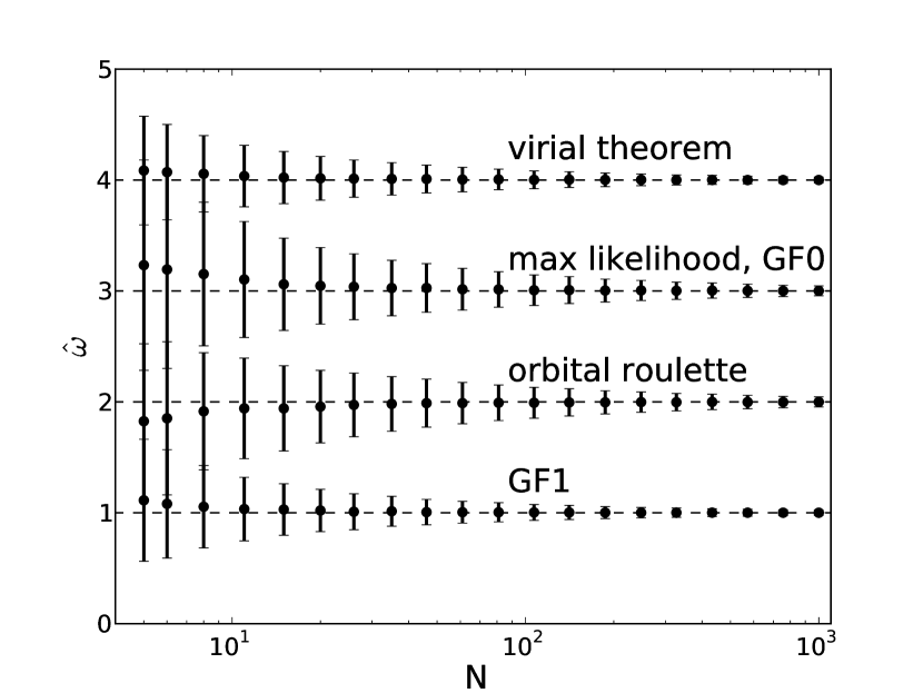
Figure 1: Performance of four estimators for $N$ particles orbiting in a harmonic potential. From top to bottom, the estimators are the virial theorem (eq. 5), the maximum-likelihood estimator (52), orbital roulette, and the minimum-variance GF1 estimator (eqs. 44 and 48). The mean estimate for the frequency $\omega$ and the standard deviation are determined for 5000 realizations and shown by the filled circles and error bars. The true frequency is $\omega=1$, and the distribution of amplitudes is given by equation (54) with $\gamma=0$ and $A_{\rm max}/A_{\rm min}=3$. To minimize confusion, the results for the different estimators have been displaced by integer offsets on the vertical axis.

The mean and standard deviation of the estimators $\hat{\omega}$ are shown in Figure 1 over the range $N=5$–1000, for a distribution of amplitudes having $\gamma=0$ and $A_{\rm max}/A_{\rm min}=3$. All four estimators exhibit modest bias for small $N$, but are consistent in the sense that the bias and standard deviation approach zero as the sample size $N\to\infty$. At $N=1000$, the standard deviations in $\hat{\omega}$, ordered by increasing magnitude, are: GF1, 0.023; then virial theorem, 0.026, then GF0, maximum likelihood, and orbital roulette tied at 0.045 (for all methods except roulette, these results can be derived analytically; see equations 6, 45, 46, and 53).

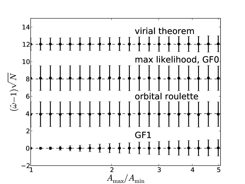
Figure 2: Performance of the same four estimators as in Figure 1 for $N=100$ particles orbiting in a harmonic potential with $\omega=1$. The distribution of amplitudes is given by equation (54) with $\gamma=0$ and varying $A_{\rm max}/A_{\rm min}$ (horizontal axis). To minimize confusion, the results for the different estimators have been displaced by integer offsets on the vertical axis. We plot $(\hat{\omega}-1)\surd{N}$, which is independent of $N$ for $N\gg 1$.

Figure 2 shows the performance of the estimators for fixed sample size $N=100$, $\gamma=0$, and a range of values for $A_{\mathrm{max}}/A_{\mathrm{min}}$. Rather than plotting $\hat{\omega}$ as in Figure 1, we plot $(\hat{\omega}-1)\surd{N}$, which is independent of sample size. The behavior of the maximum-likelihood and orbital-roulette estimators is independent of the distribution of amplitudes $A$ since they depend on the data only through the ratio $z=v/x$ (eq. 51) or $\theta$ (eq. 35) whose distributions are independent of the amplitude (this independence holds only for the harmonic potential, not for most others). In this figure, the standard deviation of the generating-function estimator GF1 is always the smallest of the four estimators. It is remarkable that the estimator GF1 performs so much better than the others when $A_{\mathrm{max}}/A_{\rm min}\sim 1$.

4 The Kepler potential

The Hamiltonian for the Kepler potential is

$$H(\textbf{{x}},\textbf{{v}}|\mu)=\textstyle{\frac{1}{2}}v^{2}+\Phi(r|\mu)=\textstyle{\frac{1}{2}}v^{2}-\frac{\mu}{r}$$ (55)

where $r=|\textbf{{x}}|$, $\mu=GM$, $G$ is the gravitational constant, and we loosely refer to $\mu$ as the mass of the central body.

An orbit is described by its semimajor axis $a$, eccentricity $e$, inclination $i$ relative to some $x$-$y$ reference plane, longitude of node $\Omega$, argument of periapsis $\omega$, and mean anomaly $\ell$. The specific angular momentum is $L=|\textbf{{x}}\times\textbf{{v}}|=[\mu a(1-e^{2})]^{1/2}$ and the $z$-component of the specific angular momentum is $L_{z}=L\cos i$. A suitable set of action-angle variables is

j $$=(j_{1},j_{2},j_{3})=\sqrt{\mu a}\Big{(}1-\sqrt{1-e^{2}},\sqrt{1-e^{2}},\sqrt{1-e^{2}}\cos i\Big{)}$$

$$=\Big{(}\sqrt{\mu a}\Big{[}1-\sqrt{1-e^{2}}\Big{]},L,L_{z}\Big{)},$$

$$\bm{\theta} =(\theta_{1},\theta_{2},\theta_{3})=(\ell,\ell+\omega,\Omega);$$ (56)

$j_{1}$ is called the radial action since it vanishes for circular orbits. In these variables the Hamiltonian is $H=-\textstyle{\frac{1}{2}}\mu^{2}/(j_{1}+j_{2})^{2}$. We shall also use the eccentric anomaly $u$, given by Kepler’s equation $\ell=u-e\sin u$.

Since the orientation of the orbit does not help to constrain the mass $\mu$, we can ignore the angles $\theta_{2}$ and $\theta_{3}$ and the action $L_{z}$. Moreover the angular momentum $L=|\textbf{{x}}\times\textbf{{v}}|$ is independent of the mass $\mu$ for fixed position and velocity $(\textbf{{x}},\textbf{{v}})$. Therefore the mass-dependent dynamics has only one degree of freedom and is described by the action $j_{1}$ and its conjugate angle $\theta_{1}$. For brevity we now drop the subscript so $j_{1}\to j$ and $\theta_{1}\to\theta=\ell$.

We have $\partial\Phi/\partial\mu=-1/r$, $r=a(1-e\cos u)$, and $d\ell=(1-e\cos u)du$ so

$$\left\langle\frac{\partial\Phi}{\partial\mu}\right\rangle_{\theta}=-\int_{0}^{2\pi}\frac{d\ell}{2\pi}\frac{1}{a(1-e\cos u)}=-\frac{1}{a},$$ (57)

and

$$\left\{\frac{\partial\Phi}{\partial\mu}\right\}_{\theta}=-\frac{1}{r}+\frac{1}{a}=-\frac{e\cos u}{a(1-e\cos u)}.$$ (58)

Then equation (30) yields the generating function

$$s_{1}(j,\theta,\mu)=\frac{(j+L)^{3}}{\mu^{2}}\int^{u}du(1-e\cos u)\left\{\frac{\partial\Phi}{\partial\mu}\right\}_{\theta}=\sqrt{\frac{a}{\mu}}e\sin u,$$ (59)

and the results

$$\partial_{2}s_{1}(j,\theta,\mu) =\sqrt{\frac{a}{\mu}}\frac{e\cos u}{1-e\cos u},$$

$$\langle[\partial_{2}s_{1}(j,\theta,\mu)]^{2}\rangle_{\theta} =\frac{a}{\mu}\left[(1-e^{2})^{-1/2}-1\right].$$ (60)

In these formulae $u$, $e$, and $a$ should be regarded as functions of the action $j=(\mu a)^{1/2}[1-(1-e^{2})^{1/2}]$, the angle $\theta=\ell=u-e\sin u$, and the angular momentum $L=[\mu a(1-e^{2})]^{1/2}$. From equations (10) and (20), the generating-function estimator of the mass is given by

$$\frac{\hat{\mu}}{\mu_{t}}=1+\frac{1}{N}\sum_{n=1}^{N}\left(1-\frac{j_{\star}}{j_{t,n}}\right)\frac{e_{t,n}(1-e_{t,n}^{2})^{1/2}\cos u_{t,n}}{1-e_{t,n}\cos u_{t,n}},$$ (61)

The estimator can be re-written in terms of observable quantities, the radius $r$, speed $v$, and radial and tangential velocities $v_{r}$ and $v_{\perp}=(v^{2}-v_{r}^{2})^{1/2}$. In making this conversion two useful identities are

$$v^{2}r=\mu(1+e\cos u),\qquad v_{r}^{2}r=\mu\frac{e^{2}\sin^{2}u}{1-e\cos u}.$$ (62)

We find

$$\frac{\hat{\mu}}{\mu_{t}}=1+\frac{1}{N}\sum_{n=1}^{N}\left(1-\frac{j_{\star}}{j_{t,n}}\right)\frac{(v_{n}^{2}r_{n}-\mu_{t})v_{\perp,n}r_{n}^{1/2}}{\mu_{t}(2\mu_{t}-v_{n}^{2}r_{n})^{1/2}}.$$ (63)

where

$$j_{t,n}=\left(\frac{r_{n}}{2\mu_{t}-v_{n}^{2}r_{n}}\right)^{1/2}\big{[}\mu_{t}-(2\mu_{t}-v_{n}^{2}r_{n})^{1/2}v_{\perp,n}r_{n}^{1/2}\big{]}.$$ (64)

The quantities within the square roots are positive so long as $2\mu_{t}\geq v_{n}^{2}r_{n}$, which holds so long as the particle is in a bound orbit at the trial mass.

The variance of the estimator $\hat{\mu}$ can be determined from equation (21) or (61). If the trial mass equals the true mass, the variance at a fixed value of the trial mass is

$$\sigma^{2} =\big{\langle}(\hat{\mu}-\langle\hat{\mu}\rangle_{\theta})^{2}\big{\rangle}_{\theta}$$

$$=\frac{\mu^{2}}{N^{2}}\sum_{n=1}^{N}\left(1-\frac{j_{\star}}{j_{n}}\right)^{2}(1-e^{2}_{n})^{1/2}\big{[}1-(1-e_{n}^{2})^{1/2}\big{]}.$$ (65)

When $j_{\star}=0$, the variance is bounded above by $\mu^{2}/(4N)$, which implies that the estimator is consistent, and by the central-limit theorem the distribution of estimates $\hat{\mu}$ is Gaussian for large $N$.

The variance is minimized when we choose

$$j_{\star} =j_{\mathrm{min}}=\mu^{1/2}\frac{\sum_{n}(1-e_{n}^{2})^{1/2}a_{n}^{-1/2}}{\sum_{n}(1-e_{n}^{2})^{1/2}a_{n}^{-1}\big{[}1-(1-e_{n}^{2})^{1/2}\big{]}^{-1}}$$ (66)

$$=\frac{\sum_{n}(2\mu-v_{n}^{2}r_{n})v_{\perp,n}}{\sum_{n}(2\mu-v_{n}^{2}r_{n})^{3/2}v_{\perp,n}\big{[}\mu r_{n}^{1/2}-(2\mu-v_{n}^{2}r_{n})^{1/2}v_{\perp,n}r_{n}\big{]}^{-1}}.$$

The estimate has converged when $\hat{\mu}=\mu_{t}$, which occurs when

$$\sum_{n=1}^{N}\left(1-\frac{j_{\star}}{j_{\hat{\mu},n}}\right)\frac{(v_{n}^{2}r_{n}-\hat{\mu})v_{\perp,n}r_{n}^{1/2}}{(2\hat{\mu}-v_{n}^{2}r_{n})^{1/2}}=0.$$ (67)

When $j_{\star}=0$ the estimator (67) simplifies to

$$\sum_{n=1}^{N}\frac{(v_{n}^{2}r_{n}-\hat{\mu})v_{\perp,n}r_{n}^{1/2}}{(2\hat{\mu}-v_{n}^{2}r_{n})^{1/2}}=0,$$ (68)

and we denote the estimator based on this formula as GF0. We denote the minimum-variance estimator based on equations (67) and (66) as GF1. Note that the generating-function estimators are unbiased, and their variance is given by (65), only for a fixed value of the trial mass. When iterated to convergence there will generally be a small non-zero bias, and the variance will be larger.

The smallest allowed mass is $\hat{\mu}_{\rm min}=\textstyle{\frac{1}{2}}v^{2}_{m}r_{m}$ where $m$ is the index corresponding to the smallest of $\{v_{n}^{2}r_{n}\}$. As $\hat{\mu}\to\hat{\mu}_{\rm min}$ from above, the left side of (68) approaches $2^{-3/2}v_{m}^{2}v_{\perp,m}r_{m}^{3/2}(\hat{\mu}-\hat{\mu}_{\rm min})^{-1/2}\to+\infty$. As $\hat{\mu}\to\infty$, the left side approaches $-2^{-1/2}{\hat{\mu}}^{1/2}\sum_{n}v_{\perp,n}r_{n}^{1/2}\to-\infty$. Moreover the left side is a monotonically decreasing function of $\hat{\mu}$. Therefore (68) has one and only one solution for $\hat{\mu}$.

When $j_{\star}\not=0$ there may be more than one solution to (67). To determine which one to use, we first find the unique solution $\hat{\mu}_{0}$ with $j_{\star}=0$, then find all the solutions with the chosen value of $j_{\star}$ and choose the one that is closest to $\hat{\mu}_{0}$.

These results are derived from the action-angle variables (56). Other sets of action-angle variables yield different estimators. For example, if we choose Delaunay elements

j $$=\sqrt{\mu a}\Big{(}1,\sqrt{1-e^{2}},\sqrt{1-e^{2}}\cos i\Big{)}=(\sqrt{\mu a},L,L_{z}),$$

$$\bm{\theta} =(\ell,\omega,\Omega),$$ (69)

the estimator analogous to (68) is

$$\sum_{n=1}^{N}\frac{(v_{n}^{2}r_{n}-\hat{\mu})v_{\perp,n}r_{n}^{1/2}}{(2\hat{\mu}-v_{n}^{2}r_{n})^{1/2}\big{[}\hat{\mu}-v_{\perp,n}r_{n}^{1/2}(2\hat{\mu}-v_{n}^{2}r_{n})^{1/2}\big{]}}=0.$$ (70)

In general this performs less well than (68). For example, if the estimated mass is correct and the orbits are circular, then $\hat{\mu}=\mu$ and $v_{n}^{2}r_{n}=v_{\perp,n}^{2}r_{n}=\mu$, so both the numerator and denominator in each term of (70) vanish.

4.1 Numerical tests

Our tests are similar to those in §3.2 for the harmonic potential. We generate 5000 realizations of the positions and velocities $\{\textbf{{x}}_{n},\textbf{{v}}_{n}\}$ of $N$ particles orbiting in a point-mass potential with unit mass, $\mu=1$. The particles are distributed uniformly random in phase, and randomly in the semimajor axis $a$ with probability density

$$dp\propto a^{-\gamma}\,d\log a,\qquad a_{\rm min}<a<a_{\rm max},$$ (71)

and zero otherwise. We have conducted tests with a variety of eccentricity distributions. We compare several estimators:

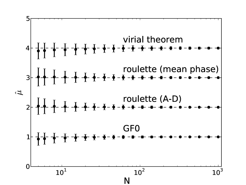
Figure 3: Performance of estimators for $N$ particles orbiting in a Kepler potential with mass $\mu=1$. The squared eccentricities are distributed uniformly random between 0 and 1. From top to bottom, the estimators are the virial theorem (eq. 7), orbital roulette using the mean phase, orbital roulette using the Anderson–Darling test, and the simple generating-function estimator GF0 ($j_{\star}=0$; eq. 68). The mean estimate for the mass and the standard deviation in $\hat{\mu}$ are determined for 5000 realizations and shown by the filled circles and error bars. The distribution of semimajor axes is given by equation (71) with $\gamma=0$ and $a_{\rm max}/a_{\rm min}=3$. To minimize confusion, the results for the different estimators have been displaced by integer offsets on the vertical axis.

1. the virial theorem (eq. 7);

2. orbital roulette, using both the mean-phase test and the Anderson–Darling test as described by Beloborodov & Levin (2004);

3. the simple generating-function estimator GF0 ($j_{\star}=0$, eq. 68) and the minimum-variance estimator GF1 ($j_{\star}=j_{\rm min}$, eqs. 67 and 66);

4. if the particles have a known eccentricity $e$ then two unbiased estimators of the mass are

   $$\hat{\mu} =\frac{1}{N(1-\textstyle{\frac{1}{2}}e^{2})}\sum_{n=1}^{N}v_{n}^{2}r_{n},$$ (72)

   $$\hat{\mu} =\frac{2}{Ne^{2}}\sum_{n=1}^{N}v_{r,n}^{2}r_{n},$$ (73)

   These estimators are not useful in practice since the eccentricities are not known, but they provide a useful benchmark for assessing the performance of other estimators (see, e.g., An & Evans, 2011).

The mean and standard deviation of the virial-theorem and orbital-roulette estimators, and of the generating-function estimator GF0 are shown in Figure 3 over the range $N=5$–1000, for a distribution of semimajor axes having $\gamma=0$ and $a_{\rm max}/a_{\rm min}=3$. In these simulations the squared eccentricity is distributed uniformly random between 0 and 1, corresponding to a df that is constant on an energy surface in canonical phase space. At $N=1000$ the standard deviations in $\hat{\mu}$, ordered by increasing magnitude, are: GF0, 0.013; orbital roulette using the Anderson–Darling test, 0.018; orbital roulette using the mean phase, 0.022; and virial theorem, 0.031. Thus the performance of GF0 is substantially better than the other estimators. Note that the GF0 estimator is independent of the distribution of semimajor axes in the sample, and its superior performance holds for a wide range of possible semimajor axis distributions.

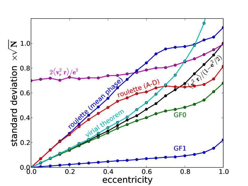
Figure 4: Performance of estimators $\hat{\mu}$ for 100 particles orbiting in a Kepler potential, all with the same eccentricity (horizontal axis). The standard deviation of $\hat{\mu}$, multiplied by $\sqrt{100}$ to provide a quantity independent of the number of particles, is plotted on the vertical axis for each of the following: virial theorem (eq. 7, cyan line); estimator based on the mean of $v^{2}r$ (eq. 72, black line); estimator based on the mean of $v_{r}^{2}r$ (eq. 73, magenta line); orbital roulette using the mean phase (blue line); orbital roulette using the Anderson–Darling test (red line); the generating-function estimator GF0 ($j_{\star}=0$; eq. 68, green line); and the generating-function estimator GF1 ($j_{\star}=j_{\mathrm{min}}$, blue line). The standard deviation is measured from 5000 realizations. The true mass is $\mu=1$, and the distribution of semimajor axes is given by equation (71) with $\gamma=0$ and $a_{\rm max}/a_{\rm min}=3$. The results plotted near $e=0$ and $e=1$ are for $e=0.0001$ and $e=0.9999$.

The minimum-variance estimator GF1 does not perform significantly better than GF0 in these simulations. The reason can be traced to equation (66) for $j_{\mathrm{min}}$. In these simulations we have assumed that the probability distribution of the squared eccentricity is uniform, $dp=de^{2}$. Then for a given semimajor axis, the mean of the denominator in the expression for $j_{\mathrm{min}}$ is proportional to $\int_{0}^{1}de\,e(1-e^{2})^{1/2}[1-(1-e^{2})^{1/2}]^{-1}$, which diverges logarithmically at its lower limit. Thus in any large sample $j_{\mathrm{min}}$ will be small, so the estimator GF1 will perform similarly to GF0. On the other hand, for a sample of particles with fixed non-zero eccentricity GF1 performs remarkably well. This is illustrated in Figure 4, which shows the normalized standard deviation (i.e., the standard deviation times $\surd N$) of several mass estimators as a function of the eccentricity. GF1 is much more accurate than any of its competitors.

A final test, motivated by Bovy et al. (2010), is to ask how well the generating-function estimators would predict the solar mass, given a snapshot of the positions and velocities of the eight planets in the solar system. Given the current semimajor axes and eccentricities of the planets, sampling the positions and velocities at a random time and applying the estimator GF0 yields the correct solar mass with a fractional standard deviation of 2.1 per cent. Using the positions and velocities on 2009 April 1 (taken from Table 1 of Bovy et al. 2010) yields $\hat{\mu}/(GM_{\odot})=1.028$. Thus, GF0 provides mass estimates accurate to within about 3 per cent in this case, even though it is given only 8 data points and no prior information on the eccentricity or semimajor axis distributions.

5 Discussion

These results offer encouraging evidence of the power of these estimators, but unanswered questions remain.

Can the generating-function estimators be derived from a maximum-likelihood approach? A possible signpost is that the GF0 estimator in a harmonic potential yields the maximum likelihood of the frequency $\omega$ for the data set $\{v_{n}/x_{n}\}$, the unique combination of positions and velocities that has the same dimension as $\omega$ (see discussion at the end of §3.1). However, no analogous result is known for most other potentials, including the Kepler potential.

What is the relation of the generating-function approach to Bayesian estimates of the posterior distribution of the mass parameters given the data (e.g., Bovy et al., 2010)?

We have shown that the generating-function estimators perform better than other distribution-free estimators such as the virial theorem or orbital roulette when applied to the harmonic or Kepler potentials. We have also shown that they avoid the conceptual difficulties associated with methods that estimate the distribution function simultaneously with the mass parameters, such as Schwarzschild’s method. We have not, however, directly compared the efficiency of the latter methods to the efficiency of generating-function estimators when applied to the same data.

In practical problems of mass estimation in astrophysics, the data are often available only over a subset of the volume occupied by the stellar system, either because of the limited field of view of the survey or because of crowding near the core or background contamination in the outskirts. How can generating-function estimators be modified to account for both incomplete phase-space sampling and observational errors?

A difficult problem arises when not all of the phase-space coordinates are known, typically because the distance along the line of sight cannot be determined accurately, and the proper motions are too small to be detectable. Can the generating-function estimators be generalized to the case where only some of the six phase-space coordinates of the particle are known?

6 Summary

We have described a novel method based on generating functions for estimating the mass parameters of a gravitational potential, given that we have positions and velocities for a set of test particles orbiting in the potential in a steady state (i.e., with random phases). The method we describe is (i) distribution-free, in the sense that it requires no prior assumptions about the distribution of the particles in action space; (ii) iterative, in the sense that it produces an estimate $\hat{\mu}$ for the mass given a trial value $\mu_{t}$, (iii) unbiased, in the sense of equation (11). In practice we iterate the estimate until $\hat{\mu}=\mu_{t}$ (eq. 25). We have demonstrated that this estimator is more powerful than other distribution-free estimators in the harmonic and Kepler potentials.

These results point the way towards more efficient and reliable mass estimators that could have broad applications in astrophysical dynamics.

Appendix A Estimators for systems with multiple mass parameters and multiple degrees of freedom

A.1 Generalization to several mass parameters

The results of §2 can be generalized to systems with $M>1$ mass parameters $\bm{\mu}=(\mu_{1},\ldots,\mu_{M})$ and one degree of freedom. The true but unknown mass parameters are described by the vector $\bm{\mu}$, and we choose a trial vector $\bm{\mu}_{t}$ that is close to $\bm{\mu}$, with $\Delta\bm{\mu}\equiv\bm{\mu}-\bm{\mu}_{t}$. The estimator of $\bm{\mu}$ is (cf. eq. 10)

$$\hat{\bm{\mu}}=\bm{\mu}_{t}+\frac{1}{N}\sum_{n=1}^{N}\textbf{{P}}(j_{t,n},\theta_{t,n},\bm{\mu}_{t})$$ (74)

and we require that the estimator is consistent and unbiased up to errors of $\mbox{O}(|\Delta\bm{\mu}|^{2})$. The analog to the generating function in equation (16) is

$$s(j,\theta_{t},\bm{\mu}_{t},\Delta\bm{\mu})=\sum_{\alpha=1}^{M}\Delta\mu_{\alpha}s_{\alpha}(j,\theta_{t},\bm{\mu}_{t})+\mbox{O}(\Delta\mu)^{2},$$ (75)

and the condition on a component of the vector P analogous to (17) is

$$\langle P_{\alpha}\rangle_{\theta}+\sum_{\beta=1}^{M}\Delta\mu_{\beta}\langle(\partial_{1}P_{\alpha})(\partial_{2}s_{\beta})-(\partial_{2}P_{\alpha})(\partial_{1}s_{\beta})\rangle_{\theta}$$

$$=\Delta\mu_{\alpha}+\mbox{O}(\Delta\mu)^{2};$$ (76)

in this equation the arguments of all functions are $(j,\theta,\bm{\mu}_{t})$. Let

$$P_{\alpha}(j,\theta,\bm{\mu})=\sum_{\gamma=1}^{M}c_{\alpha\gamma}(j,\bm{\mu})\partial_{2}s_{\gamma}(j,\theta,\bm{\mu});$$ (77)

then $\langle P_{\alpha}\rangle_{\theta}=0$ and equation (76) simplifies to

$$\sum_{\gamma=1}^{M}\frac{\partial}{\partial j}c_{\alpha\gamma}(j,\bm{\mu})S_{\gamma\beta}(j,\bm{\mu})=\delta_{\alpha\beta}$$ (78)

where

$$S_{\gamma\beta}(j,\bm{\mu})=\langle\partial_{2}s_{\gamma}\,\partial_{2}s_{\beta}\rangle_{\theta}.$$ (79)

Now let $\textbf{{S}}^{-1}$ denote the inverse of the $M\times M$ matrix S with components $S_{\alpha\gamma}$. If we set $c_{\alpha\gamma}=(j-j_{\star})\,S^{-1}_{\alpha\gamma}$ then equation (79) is satisfied, and a suitable estimator is given by (74) with

$$P_{\alpha}=(j-j_{\star})\sum_{\gamma=1}^{M}S^{-1}_{\alpha\gamma}\,\partial_{2}s_{\gamma}(j,\theta,\bm{\mu}).$$ (80)

A.2 Generalization to several degrees of freedom

Now suppose that there is a single mass parameter $\mu$ and $D>1$ degrees of freedom, so the actions and angles become $D$-dimensional vectors $(\textbf{{j}},\bm{\theta})$. The analog to equation (17) is

$$\langle P\rangle_{\theta}+\Delta\mu\sum_{k=1}^{D}\left\langle\frac{\partial P}{\partial j_{k}}\frac{\partial s_{1}}{\partial\theta_{k}}-\frac{\partial P}{\partial\theta_{k}}\frac{\partial s_{1}}{\partial j_{k}}\right\rangle_{\!\bm{\theta}}=\Delta\mu+\mbox{O}(\Delta\mu)^{2};$$ (81)

here the average $\langle\cdot\rangle_{\bm{\theta}}$ is over all of the $D$ angles. Let us write

$$P(\textbf{{j}},\bm{\theta},\mu)=\sum_{i}q_{i}(\textbf{{j}},\bm{\theta},\mu)\,\partial s_{1}(\textbf{{j}},\bm{\theta},\mu)/\partial\theta_{i}.$$ (82)

Then equation (81) requires

$$\sum_{k,i=1}^{D}\frac{\partial}{\partial j_{k}}T_{ki}(\textbf{{j}},\mu)q_{i}(\textbf{{j}},\mu)=1,\ \ \mbox{where}\ \ T_{ki}(\textbf{{j}},\mu)=\left\langle\frac{\partial s_{1}}{\partial\theta_{k}}\frac{\partial s_{1}}{\partial\theta_{i}}\right\rangle_{\!\bm{\theta}}.$$ (83)

This condition is satisfied if

$$q_{i}(\textbf{{j}},\mu)=\sum_{m=1}^{D}T^{-1}_{im}\alpha_{m}(j_{m}-j_{m}^{\star})\quad\mbox{where}\quad\sum_{m=1}^{D}\alpha_{m}=1.$$ (84)

where $\textbf{{T}}^{-1}$ is the inverse of the matrix T and $\textbf{{j}}^{\star}\}$ is a constant vector.

A.3 Generalization to several mass parameters and degrees of freedom

It is straightforward to generalize the preceding results to systems with $M>1$ mass parameters and $D>1$ degrees of freedom. The analogs to equations (74)–(76) are

$$\hat{\bm{\mu}}=\bm{\mu}_{t}+\frac{1}{N}\sum_{n=1}^{N}\textbf{{P}}(\textbf{{j}}_{t,n},\bm{\theta}_{t,n},\bm{\mu}_{t});$$ (85)

$$s(\textbf{{j}},\bm{\theta}_{t},\bm{\mu}_{t},\Delta\bm{\mu})=\sum_{\alpha=1}^{M}\Delta\mu_{\alpha}s_{\alpha}(\textbf{{j}},\bm{\theta}_{t},\bm{\mu}_{t})+\mbox{O}(\Delta\mu)^{2},$$ (86)

$$\langle P_{\alpha}\rangle_{\theta}+\sum_{\beta=1}^{M}\Delta\mu_{\beta}\sum_{k=1}^{D}\left\langle\frac{\partial P_{\alpha}}{\partial j_{k}}\frac{\partial s_{\beta}}{\partial\theta_{k}}-\frac{\partial P_{\alpha}}{\partial\theta_{k}}\frac{\partial s_{\beta}}{\partial j_{k}}\right\rangle_{\bm{\theta}}$$

$$=\Delta\mu_{\alpha}+\mbox{O}(\Delta\mu)^{2}.$$ (87)

Here $P_{\alpha}$ is a component of an $M$-dimensional vector $\textbf{{P}}(\textbf{{j}},\bm{\theta},\bm{\mu})$. We choose this to have the form

$$P_{\alpha}(\textbf{{j}},\bm{\theta},\bm{\mu})=\sum_{\gamma=1}^{M}\sum_{i=1}^{D}Q_{\alpha i\gamma}(\textbf{{j}},\bm{\theta},\bm{\mu})\frac{\partial s_{\gamma}(\textbf{{j}},\bm{\theta},\bm{\mu})}{\partial\theta_{i}}.$$ (88)

The condition (87) becomes

$$\sum_{\gamma=1}^{M}\sum_{i,k=1}^{D}\frac{\partial}{\partial j_{k}}Q_{\alpha i\gamma}(\textbf{{j}},\bm{\theta},\bm{\mu})U_{i\gamma k\beta}(\textbf{{j}},\bm{\theta},\bm{\mu})=\delta_{\alpha\beta}$$ (89)

where

$$U_{i\gamma k\beta}\equiv\left\langle\frac{\partial s_{\gamma}}{\partial\theta_{i}}\frac{\partial s_{\beta}}{\partial\theta_{k}}\right\rangle_{\bm{\theta}}.$$ (90)

Now introduce a multi-index $\mathfrak{i}$ where each $\mathfrak{i}$ corresponds to a 2-tuple $(i,\gamma)$. Similarly the indices $\mathfrak{k}$ and $\mathfrak{m}$ correspond to the pairs $(k,\beta)$ and $(m,\alpha)$ respectively. Then equation (90) can be rewritten

$$\sum_{k=1}^{D}\frac{\partial}{\partial j_{k}}\sum_{\mathfrak{i}\leq(D,M)}Q_{\alpha\mathfrak{i}}(\textbf{{j}},\bm{\theta},\bm{\mu})U_{\mathfrak{ik}}(\textbf{{j}},\bm{\theta},\bm{\mu})=\delta_{\alpha\beta}.$$ (91)

If we set

$$Q_{\alpha\mathfrak{i}}(\textbf{{j}},\bm{\theta},\bm{\mu})\equiv\sum_{m=1}^{D}\alpha_{m}(j_{m}-j^{\star}_{m})U^{-1}_{\mathfrak{mi}}(\textbf{{j}},\bm{\theta},\bm{\mu})\ \ \mbox{where}\ \ \sum_{m=1}^{D}\alpha_{m}=1,$$ (92)

then the left side of equation (91) becomes

$$\sum_{k,m=1}^{D}\frac{\partial}{\partial j_{k}}\alpha_{m}(j_{m}-j^{\star}_{m})\sum_{\mathfrak{i}\leq(D,M)}^{DM}U^{-1}_{\mathfrak{mi}}((\textbf{{j}},\bm{\theta},\bm{\mu})U_{\mathfrak{ik}}(\textbf{{j}},\bm{\theta},\bm{\mu})$$

$$=\sum_{k,m=1}^{D}\frac{\partial}{\partial j_{k}}\alpha_{m}(j_{m}-j^{\star}_{m})\delta_{\alpha\beta}\delta_{mk}=\delta_{\alpha\beta}$$ (93)

so condition (91) is satisfied.

References

• Aaronson (1983) Aaronson, M. 1983, ApJ, 266, L11
• An & Evans (2011) An, J. H., & Evans, N. W. 2011, MNRAS, 413, 1744
• Bahcall & Tremaine (1981) Bahcall, J. N., & Tremaine, S. 1981, ApJ, 244, 805
• Beloborodov & Levin (2004) Beloborodov, A. M., & Levin, Y. 2004, ApJ, 613, 224
• Bovy et al. (2010) Bovy, J., Murray, I., & Hogg, D. W. 2010, ApJ, 711, 1157
• Chakrabarty & Saha (2001) Chakrabarty, D., & Saha, P. 2001, AJ, 122, 232
• Feldmeier-Krause et al. (2017) Feldmeier-Krause, A., Zhu, L., Neumayer, N., et al. 2017, MNRAS, 466, 4040
• Kapteyn (1922) Kapteyn, J. C. 1922, ApJ, 55, 302
• Lancaster (2000) Lancaster, T. 2000, J. Econometrics, 95, 391
• Magorrian (2006) Magorrian, J. 2006, MNRAS, 373, 425
• Magorrian (2014) Magorrian, J. 2014, MNRAS, 437, 2230
• McConnachie (2012) McConnachie, A. W. 2012, AJ, 144, 4
• Neyman & Scott (1948) Neyman, J., & Scott, E. L. 1948, Econometrica 16, 1
• Zwicky (1933) Zwicky, F. 1933, Helvetica Physica Acta, 6, 110