Theory of type-II superconductivity in ferromagnetic metals with triplet pairing

Abstract

The superconducting state in uranium compounds UGe₂, URhGe and UCoGe is formed at temperatures far below the Curie temperature pointing on nonconventional nature of superconductivity in these materials - namely the superconductivity with triplet pairing. The emergence of superconductivity is accompanied by the slight magnetization expulsion typical for the type-II superconductors. Following classic Abrikosov paper I develop the theory of type-II superconductivity in application to two-band ferromagnetic metal with equal spin triplet pairing.

Key words: ferromagnetism, superconductivity

I Introduction

The investigations of interplay between superconductivity and magnetism have long story. Usually ferromagnetic ordering suppresses the superconducting state because the exchange field exceeds the paramagnetic limit field and aligns the electron spins directed oppositely in Cooper pairs. Nevertheless, singlet superconductivity can coexist with ferromagnetism when the critical temperature of the transition to the superconducting state is greater than the Curie temperature, as is the case with ternary compounds investigated in the 1980s (for review see Maple1995 ). The coexistence occurs in a form crypto-ferromagnetic superconducting state characterized by appearance a periodic magnetic structure with period larger than the interatomic distance, but smaller than the superconducting coherence length, which weakens the depairing effect of the exchange field.

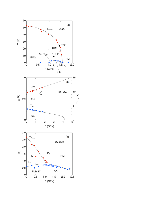
Figure 1: (Color online) Temperature-pressure phase diagram of UGe2, URhGe, and UCoGe. Notations FM, SC and PM have been used for ferromagnetic, superconducting and paramagnetic phases correspondingly, TCP is the tricritical point, CEP is the critical end point. Aoki2014

The superconductivity in the more recently discovered uranium compounds UGe₂, URhGe and UCoGe Saxena01 ; Aoki01 ; Huy07 exhibits quite different properties (see the experimental Aoki2014 and theoretical reviews Mineev2016 and references therein). Here the superconducting states exist at temperatures far below the Curie temperature Fig.1 and in the magnetic fields strongly exceeding the paramagnetic limit indicating that we deal with the triplet pairing. The general form of superconducting order parameters in these orthorhombic compounds is found in the paper Mineev2002 . Similar to the superfluid ³He the pairing interaction is caused by the magnetic fluctuations. The theory based on this mechanism and on the symmetry considerations allows explain many specific properties of these materials Mineev2016 .

Quite recently there was proposed the phenomenological description of the phase diagram of UCoGe Raghu2016 ; Mineev2017 where the ferromagnetism is suppressed by pressure whereas the superconductivity arising at small pressures inside of the ferromagnetic state continues to exist at high pressures in the paramagnetic state Fig.1c. The theory was developed as if it would be in the neutral superfluid. This approach is justified by the smallness of the internal magnetic field interacting with the electron charges that slightly changes the critical temperature of transition to the superconducting state. The effects caused by the screening supercurrents has been taken into account only qualitatively Mineev2017 . This has allowed to explain the significant difference between the transition from the ferromagnetic to the ferromagnetic superconducting state and the transition from the superconducting to the ferromagnetic superconducting state. However, the developed theory was not completely consistent.

All the aforementioned superconductors are related to the type-II superconducting materials Dao2011 . The internal magnetic fields in all of them exceed the corresponding lower critical fields $H_{c1}$ Aoki2014 ; Deguchi2010 ; Paulsen2012 ; Hykel2014 . Hence, at temperature decrease the phase transition from the ferromagnetic to the ferromagnetic superconducting state occurs to the mixed state characterized by the emergence of Abrikosov vortices. Accordingly, the proper theory of this phase transition must be formulated in frame Ginzburg-Landau-Abrikosov theory of type-II superconductivity Abrikosov1957 . In the application to ferromagnetic conventional superconductors with singlet pairing such approach has been developed first in the papers Blount1979 ; Kuper1980 . The corresponding theory for the nonmagnetic superconductors with equal spin triplet pairing in absence of spin-orbital coupling has been presented in the paper Agterberg2009 .

Here, I develop the Abrikosov theory of type-II superconductivity for equal spin pairing triplet superconducting state in two band ferromagnetic metal. First, I describe the phase transition from ferromagnetic to superconducting ferromagnetic state that occurs in all three uranium compounds (see Fig.1). Then I consider the solution for isolated vortex in such type superconductors and the transition from the Meissner to the mixed superconducting state which is realized in UCoGe. In my derivation I use the pedagogic presentation of classic Abrikosov theory performed by N.B.Kopnin Kopnin2002 .

II Model

The triplet-pairing superconducting state order parameter in two-band (spin-up, spin-down) ferromagnet is given by the complex spin-vector Mineev2016 ; Book

$${\bf d}({\bf k},{\bf r})=~{}~{}~{}~{}~{}~{}~{}~{}~{}~{}~{}~{}~{}~{}~{}~{}~{}~{}~{}~{}~{}~{}~{}~{}~{}~{}~{}$$ (1)

$$\frac{1}{2}\left[-\Delta^{\uparrow}({\bf k},{\bf r})(\hat{x}+i\hat{y})+\Delta^{\downarrow}({\bf k},{\bf r})(\hat{x}-i\hat{y})\right]+\Delta^{0}({\bf k},{\bf r})\hat{z},$$

where $\Delta_{\uparrow}({\bf k},{\bf r})$, $\Delta_{\downarrow}({\bf r},{\bf k},{\bf r})$, $\Delta_{0}({\bf k},{\bf r})$ are the amplitudes of spin-up, spin-down and zero-spin of superconducting order parameter depending on the Cooper pair centre of gravity coordinate ${\bf r}$ and the common direction of momentum ${\bf k}$ of pairing electrons. In the orthorhombic ferromagnets with easy axis along $\hat{z}$ direction there are only two superconducting states A and B with different critical temperature Mineev2002 . We will work with equal spin pairing B-state with the order parameter

$$\Delta_{B}^{\uparrow}({\bf k},{\bf r})=\hat{k}_{z}\eta_{1}({\bf r}),$$

$$\Delta_{B}^{\downarrow}({\bf k},{\bf r})=\hat{k}_{z}\eta_{2}({\bf r}).$$ (2)

The Ginzburg-Landau free energy functional is

$$F=\int dV\left\{\alpha M^{2}+\beta M^{4}+D_{ij}\nabla_{i}M\nabla_{j}M\right.$$

$$+\left.\alpha_{1}(|\eta_{1}|^{2}+|\eta_{2}|^{2})+\gamma_{1}({\bf B}\hat{z})(|\eta_{1}|^{2}-|\eta_{2}|^{2})+\gamma_{2}(\eta_{1}\eta_{2}^{\star}+\eta_{1}^{\star}\eta_{2})+\beta_{1}(|\eta_{1}|^{4}+|\eta_{2}|^{4})+\beta_{2}|\eta_{1}|^{2}|\eta_{2}|^{2}\right.$$

$$\left.+K_{1ij}(D_{i}\eta_{1})^{\star}D_{j}\eta_{1}+K_{2ij}(D_{i}\eta_{2})^{\star}D_{j}\eta_{2}+\frac{\bf B^{2}}{8\pi}-{\bf B}{\bf M}\right\},$$ (3)

where $M$ is the density of magnetic moment component along the easy axis, ${\bf B}=curl{\bf A}$ is the magnetic induction,

$$\alpha=\alpha_{0}(T-T^{\prime}_{c}),~{}~{}~{}~{}~{}\alpha_{1}=\alpha_{10}(T-T_{sc0}),$$ (4)

$T_{c}^{\prime}(P)$ is the pressure dependent ”Curie temperature” ( see Blount1979 ) and $T_{sc0}(P)$ is the formal critical temperature of superconducting transition in the single band (say just spin-up) case. ${\bf D}=-i\hbar\nabla-\frac{2e}{c}{\bf A}$ is the long derivative. In a single domain ferromagnet in the absence of external field $H=0$ or at the external field directed along the axis of spontaneous magnetization $\hat{z}$ the order parameter components are the $z$-coordinate independent and the long derivatives are

$$D_{x}=-i\hbar\frac{\partial}{\partial x},~{}~{}D_{y}=-i\hbar\frac{\partial}{\partial y}-\frac{2e}{c}A_{y}.$$ (5)

For the superconducting state (2) the gradient terms have the following form

$$K_{1xx}(D_{x}\eta_{1})^{\star}D_{x}\eta_{1}+K_{1yy}(D_{y}\eta_{1})^{\star}D_{y}\eta_{1}+(1~{}\to~{}2).$$

The upper critical field problem in two band superconductor with different stiffness constants $K_{1xx}$ and $K_{1yy}$ can be solved only numerically or by means of variation approach used in the paper by Zhitomirsky and Dao Dao2004 . With purpose to develop the analytic treatment we neglect the orthorhombicity puting $K_{1xx}=K_{1yy}=K_{1}$, $K_{2xx}=K_{2yy}=K_{2}$ and also $D_{xx}=D_{yy}=D$.

An analytic solution can be found also for the equal spin pairing A-state

$$\Delta^{\uparrow}({\bf k},{\bf r})=\hat{k}_{x}\eta_{1}({\bf r}),$$

$$\Delta^{\downarrow}({\bf k},{\bf r})=\hat{k}_{x}\eta_{2}({\bf r}).$$ (6)

discussed in the papers Raghu2016 ; Mineev2017 . Then, however, due to the gradient mixing terms like $(D_{x}\eta_{1x})^{\star}D_{y}\eta_{1y}$ the order parameter (6) acquires (seeMineev2016 ) more general form

$$\Delta^{\uparrow}({\bf k},{\bf r})=\hat{k}_{x}\eta_{1x}({\bf r})+i\hat{k}_{y}\eta_{1y}({\bf r}),$$ (7)

$$\Delta^{\downarrow}({\bf k},{\bf r})=\hat{k}_{x}\eta_{2x}({\bf r})+i\hat{k}_{y}\eta_{2y}({\bf r}).$$ (8)

Thus, instead two GL equations for the superconducting order parameters one has to solve four of them. The linear equations for $\eta_{1x},\eta_{1y},\eta_{2x},\eta_{2y}$ can be solved making use the generalization on two band case the problem of the upper critical field in uniaxial superconductor with two-component order parameter under magnetic field directed along four-fold axis (see Book ). This, however, leads to very cumbersome equations and we prefer to work with the state given by Eq.(2) and the free energy functional

$$F=\int dV\left\{\alpha M^{2}+\beta M^{4}+D(\nabla_{x}M)^{2}+D(\nabla_{y}M)^{2}+\right.$$

$$+\left.\alpha_{1}(|\eta_{1}|^{2}+|\eta_{2}|^{2})+\gamma_{1}({\bf B}\hat{z})(|\eta_{1}|^{2}-|\eta_{2}|^{2})+\gamma_{2}(\eta_{1}\eta_{2}^{\star}+\eta_{1}^{\star}\eta_{2})+\beta_{1}(|\eta_{1}|^{4}+|\eta_{2}|^{4})+\beta_{2}|\eta_{1}|^{2}|\eta_{2}|^{2}\right.$$

$$\left.+K_{1}[(D_{x}\eta_{1})^{\star}D_{x}\eta_{1}+(D_{y}\eta_{1})^{\star}D_{y}\eta_{1}]+K_{2}[(D_{x}\eta_{2})^{\star}D_{x}\eta_{2}+(D_{y}\eta_{2})^{\star}D_{y}\eta_{2}]+\frac{\bf B^{2}}{8\pi}-{\bf B}{\bf M}\right\}.$$ (9)

III Transition from ferromagnetic to superconducting ferromagnetic state

In URhGe and UCoGe below phase transition in ferromagnetic state the magnetic moment acquires the finite value, the magnetic induction is $B=4\pi M$ and a superconducting ordering is absent

$$M^{2}=(M_{0}(T))^{2}=-\frac{\alpha_{0}(T-T_{c}(P))}{2\beta},~{}~{}~{}\eta_{1}=\eta_{2}=0,$$ (10)

where the Curie temperature is

$$T_{c}=T_{c}^{\prime}+\frac{2\pi}{\alpha_{0}}.$$ (11)

In presence of an external field $H=B-4\pi M$ parallel to spontaneous magnetization the magnetic moment is determined by the equation

$$2\alpha M_{0}+4\beta M_{0}^{3}=H.$$ (12)

At arbitrary temperatures below the Curie temperature, one can work with the GL formula for $M_{0}$ only qualitatively. Instead, it is possible to use the known experimental values of magnetization $M_{0}(H,T)$ The same is true for UGe₂ where the superconductivity arises below the first order phase transition to ferromagnetic state Fig.1.

At the subsequent phase transition the superconducting order parameter amplitudes $\eta_{1},\eta_{2}$ appear. They are determined by the Ginzburg-Landau equations obtained by variation of Eq.(9) in respect to $\eta_{1},\eta_{2}$

$$(\alpha_{1}+\gamma_{1}B)\eta_{1}-K_{1}\left[\frac{\partial^{2}}{\partial x^{2}}+\left(\frac{\partial}{\partial y}-\frac{2ieB}{\hbar c}x\right)^{2}\right]\eta_{1}+\gamma_{2}\eta_{2}+2\beta_{1}|\eta_{1}|^{2}\eta_{1}+\beta_{2}\eta_{1}|\eta_{2}|^{2}=0,$$ (13)

$$\gamma_{2}\eta_{1}+(\alpha_{1}-\gamma_{1}B)\eta_{2}-K_{2}\left[\frac{\partial^{2}}{\partial x^{2}}+\left(\frac{\partial}{\partial y}-\frac{2ieB}{\hbar c}x\right)^{2}\right]\eta_{2}+2\beta_{1}|\eta_{2}|^{2}\eta_{2}+\beta_{2}|\eta_{1}|^{2}\eta_{2}=0.$$ (14)

III.1 Upper critical field

The transition to the superconducting state occurs at $B_{c2}(T)$ which is the eigen value of the corresponding linear equations

$$(\alpha_{1}+\gamma_{1}B_{c2})\eta_{10}-K_{1}\left[\frac{\partial^{2}}{\partial x^{2}}+\left(\frac{\partial^{2}}{\partial y}-\frac{2ieB_{c2}}{\hbar c}x\right)^{2}\right]\eta_{10}+\gamma_{2}\eta_{20}=0,$$ (15)

$$\gamma_{2}\eta_{10}+(\alpha_{1}-\gamma_{1}B_{c2})\eta_{20}-K_{2}\left[\frac{\partial^{2}}{\partial x^{2}}+\left(\frac{\partial^{2}}{\partial y}-\frac{2ieB_{c2}}{\hbar c}x\right)^{2}\right]\eta_{20}=0.$$ (16)

The solution of this system for the lowest eigen value is

$$\eta_{i0}=C_{i}\exp\left[-\frac{\pi B_{c2}}{\Phi_{0}}\left(x-\frac{q\Phi_{0}}{2\pi B_{c2}}\right)^{2}\right],~{}~{}~{}~{}~{}~{}i=1,2,$$ (17)

where $\Phi_{0}=\frac{\pi\hbar c}{e}$ is the magnetic flux quantum. Substitution of solutions back to equations yields the system of linear equations for coefficients $C_{1},C_{2}$. The equality of the determinant of this system to zero yields the equation for the $B_{c2}(T)$

$$\left(\frac{2\pi B_{c2}}{\Phi_{0}}\right)^{2}+\left(\frac{\alpha_{1}+\gamma_{1}B_{c2}}{K_{2}}-\frac{\alpha_{1}-\gamma_{1}B_{c2}}{K_{1}}\right)\frac{2\pi B_{c2}}{\Phi_{0}}+\frac{\alpha_{1}^{2}-(\gamma_{1}B_{c2})^{2}-\gamma_{2}^{2}}{K_{1}K_{2}}=0.$$ (18)

It contains the terms $\alpha_{1}\pm\gamma_{1}B_{c2}=\alpha_{10}(T-T_{sc0}\pm\gamma_{1}B_{c2}/\alpha_{10})$ corresponding to the shifts of critical temperature in spin-up and spin-down bands. In a magnetic (nonunitary) superconducting state the shift of $T_{sc0}$ is much smaller than the temperature $T_{sc0}$ (seeBook ):

$$\frac{\gamma_{1}B_{c2}}{\alpha_{10}}\approx\frac{\mu_{B}B_{c2}}{\varepsilon_{F}}T_{sc0},$$ (19)

where $\mu_{B}$ is the Bohr magneton and $\varepsilon_{F}$ is the Fermi energy. In neglect these terms

$$B_{c2}(T)=\frac{\Phi_{0}}{2\pi}\left\{-\frac{\alpha_{1}}{2K_{2}}-\frac{\alpha_{1}}{2K_{1}}+\left[\left(\frac{\alpha_{1}}{2K_{2}}-\frac{\alpha_{1}}{2K_{1}}\right)^{2}+\frac{\gamma_{2}^{2}}{K_{1}K_{2}}\right]^{1/2}\right\}.$$ (20)

In the absence of external field the ferromagnet volume is filled by the domains with opposite magnetization orientation and the equation

$$B_{c2}(T_{sc})=4\pi M_{0}(T_{sc}).$$ (21)

determines the critical temperature $T_{sc}$ of transition to the superconducting state. When the external field increases the parallel to the field domains are expanded, the antiparallel domains are shrunk and the critical temperature does not change till $H=4\pi M_{0}$ Hardy2005 . When the external field exceeds $4\pi M_{0}$ the multi-domain ferromagnetic structure is suppressed. We will develop theory for phase transition to superconducting state in single ferromagnetic domain with magnetization parallel to the external field where the upper critical field at temperatures below $T_{sc}$ is determined by equation

$$H_{c2}(T)=B_{c2}(T)-4\pi M_{0}(T),$$ (22)

that near the critical temperature is

$$H_{c2}(T)=\frac{\partial(B_{c2}(T)-4\pi M_{0}(T))}{\partial T}|_{T=T_{sc}}(T-T_{sc}).$$ (23)

One must remember, however, that the actual upper critical field in multi-domain specimen at given temperature $T<T_{sc}$ is shifted up on $4\pi M$ in respect to this value (see Fig.2).

I will not write the explicit formula for $T_{sc}$ and for $\frac{\partial B_{c2}(T)}{\partial T}\left|{}_{T=T_{sc}}\right.$. They are quite cumbersome even in negligence of temperature and field dependence of magnetization $M_{0}$. A reader can easily obtain them.

III.2 Vortex lattice

The solution (17) is centered at $x=\hbar cq/2eB_{c2}=q\Phi_{0}/2\pi B_{c2}$. The full solution is a linear combination of these solutions for different $q$. One can construct a periodic solution of the form

$$\eta_{i0}=\sum_{n}C_{i,n}\exp\left[iqny-\frac{\pi B_{c2}}{\Phi_{0}}\left(x-\frac{qn\Phi_{0}}{2\pi B_{c2}}\right)^{2}\right],~{}~{}~{}~{}~{}~{}i=1,2.$$ (24)

It is periodic in $y$ with period $Y_{0}=2\pi/q$. It would be periodic in $x$ as well if the coefficients satisfy the periodicity condition $C_{i,n+p}=C_{i,n}$, where $p$ is an integer. Then,

$$\eta_{i0}\left(x+\frac{p\hbar cq}{2eB_{c2}},y\right)=e^{ipqy}\eta_{i0}(x,y)$$ (25)

The simplest case is realized when all the coefficients $C_{i,n}=C_{i}$ are $n$-independent. The array forms a rectangular lattice.

The modulus of these distributions are double periodic with periods

$$X_{0}=\frac{\hbar cq}{2eB_{c2}},~{}~{}~{}~{}Y_{0}=\frac{2\pi}{q}.$$

The unit cell area of rectangular lattice is

$$X_{0}Y_{0}=\frac{\Phi_{0}}{B_{c2}}=2\pi\xi^{2},$$ (26)

which corresponds to exactly one flux quantum per unit cell. If $q$ is chosen in such a way that $X_{0}=Y_{0}$, we obtain a square lattice.

III.3 Magnetization decrease below transition to the superconducting ferromagnetic state

At magnetic field $H$ slightly below $H_{c2}(T)$ there is the screening of magnetization by superconducting currents. This case the superconducting order parameter amplitudes and the ferromagnetic moment acquire the small correction

$$\eta_{1}=\eta_{10}+\tilde{\eta}_{1},~{}~{}~{}~{}\eta_{2}=\eta_{20}+\tilde{\eta}_{2},~{}~{}~{}~{}~{}{\bf M}=M_{0}\hat{z}+m({\bf r})\hat{z}.$$ (27)

The same is true for the vector-potential which is

$${\bf A}={\bf A}_{0}+{\bf A}_{1},~{}~{}~{}~{}{\bf A}_{0}=(0,B_{c2}x,0),~{}~{}~{}~{}{\bf A}_{1}=(0,(H+4\pi M_{0}-B_{c2})x,0)+\delta{\bf A}({\bf r}).$$ (28)

The corresponding magnetic induction is

$${\bf B}=curl{\bf A}==(H+4\pi M_{0})\hat{z}+\delta B({\bf r})\hat{z}.$$ (29)

It is important to note that in the ferromagnetic superconducting mixed state the specimen magnetization is not equal to $M=M_{0}+m({\bf r})$ but

$${\cal M}=\frac{\langle(B-H)\rangle}{4\pi}=M_{0}+\frac{\langle\delta B({\bf r})\rangle}{4\pi}.$$ (30)

where $\langle(\dots)\rangle=S^{-1}\int dxdy(\dots)$ is the space average over the surface perpendicular to spontaneous magnetization.

By variation of the functional Eq.(9) in respect to the vector potential we obtain the Maxwell equation

$$\frac{c}{4\pi}curl[\delta{\bf B}-4\pi{\bf m}+4\pi\hat{z}\gamma_{1}(|\eta_{10}|^{2}-|\eta_{20}|^{2})]={\bf j}=-\frac{2ie}{\hbar c}K_{1}\left[\eta_{10}^{\star}(\nabla-\frac{2ie}{\hbar c}{\bf A}_{0})\eta_{10}-\eta_{10}(\nabla+\frac{2ie}{\hbar c}{\bf A}_{0})\eta_{10}^{\star}\right]+(1\to 2)$$ (31)

or

$$\frac{c}{4\pi}\frac{\partial[\delta B-4\pi m+4\pi\gamma_{1}(|\eta_{10}|^{2}-|\eta_{20}|^{2})]}{\partial y}=j_{x}=-\frac{2e}{\hbar}\left\{K_{1}\left(i\eta_{10}^{\star}\frac{\partial\eta_{10}}{\partial x}-i\eta_{10}\frac{\partial\eta_{10}^{\star}}{\partial x}\right)+(1\to 2)\right\},$$ (32)

$$-\frac{c}{4\pi}\frac{\partial[\delta B-4\pi m+4\pi\gamma_{1}(|\eta_{10}|^{2}-|\eta_{20}|^{2})]}{\partial x}=j_{y}=-\frac{2e}{\hbar}\left\{K_{1}\left(\eta_{10}^{\star}(i\frac{\partial}{\partial x}+\frac{2\pi B_{c2}}{\Phi_{0}})\eta_{10}-\eta_{10}(i\frac{\partial}{\partial x}-\frac{2\pi B_{c2}}{\Phi_{0}})\eta_{10}^{\star}\right)+(1\to 2)\right\}.$$ (33)

With help of relation

$$\frac{\partial\eta_{i0}}{\partial x}=\left(-i\frac{\partial}{\partial y}-\frac{2\pi B_{c2}}{\Phi_{0}}\right)\eta_{i0}$$

one can rewrite the Maxwell equations as

$$\frac{\partial[\delta B-4\pi m+4\pi\gamma_{1}(|\eta_{10}|^{2}-|\eta_{20}|^{2})]}{\partial y}=-4\pi\frac{2\pi}{\Phi_{0}}\left(K_{1}\frac{\partial|\eta_{10}|^{2}}{\partial y}+K_{2}\frac{\partial|\eta_{20}|^{2}}{\partial y}\right),$$ (34)

$$\frac{\partial[\delta B-4\pi m+4\pi\gamma_{1}(|\eta_{10}|^{2}-|\eta_{20}|^{2})]}{\partial x}=-4\pi\frac{2\pi}{\Phi_{0}}\left(K_{1}\frac{\partial|\eta_{10}|^{2}}{\partial x}+K_{2}\frac{\partial|\eta_{20}|^{2}}{\partial x}\right).$$ (35)

Hence,

$$\delta B=-4\pi\frac{2\pi}{\Phi_{0}}\left(K_{1}|\eta_{10}|^{2}+K_{2}|\eta_{20}|^{2}\right)+4\pi m-4\pi\gamma_{1}(|\eta_{10}|^{2}-|\eta_{20}|^{2}).$$ (36)

Now, let us find $m({\bf r})$. Below $T_{sc}$ the magnetization is determined from the equation

$$2\alpha M+4\beta M^{3}-2D\Delta M-B=0,$$ (37)

obtained by the variation of the functional Eq.(9) in respect to $M$. Here $\Delta$ is the 2D Laplacean. Hence, the correction to magnetization $m=M-M_{0}$ is determined by the equation

$$(2\alpha+12\beta M_{0}^{2}-2D\Delta)m=\delta B$$ (38)

which, taking into account Eq.(36), can be rewritten as

$$(2\tilde{\alpha}+12\beta M^{2}-2D\Delta)m=-4\pi\frac{2\pi}{\Phi_{0}}\left(K_{1}|\eta_{10}|^{2}+K_{2}|\eta_{20}|^{2}\right)-4\pi\gamma_{1}(|\eta_{10}|^{2}-|\eta_{20}|^{2}),$$ (39)

where $\tilde{\alpha}=\alpha_{0}(T-T_{c})=\alpha_{0}(T-T_{c}^{\prime}-2\pi/\alpha_{0})$. The magnetic coherence length is much shorter than the size of vortex lattice cell

$$\xi_{m}=\frac{\sqrt{D}}{\sqrt{\tilde{\alpha}+6\beta M^{2}}}<<\xi.$$

Hence,

$$m({\bf r})=-\frac{\frac{(2\pi)^{2}}{\Phi_{0}}\left(K_{1}|\eta_{10}|^{2}+K_{2}|\eta_{20}|^{2}\right)+2\pi\gamma_{1}(|\eta_{10}|^{2}-|\eta_{20}|^{2})}{\tilde{\alpha}+6\beta M_{0}^{2}}.$$ (40)

According to Eq.(30) the magnetization decrease below transition to the superconducting state is

$${\cal M}-M_{0}=\frac{\langle\delta B({\bf r})\rangle}{4\pi}=-\left\langle\frac{2\pi}{\Phi_{0}}\left(K_{1}|\eta_{10}({\bf r})|^{2}+K_{2}|\eta_{20}({\bf r})|^{2}\right)-m({\bf r})+\gamma_{1}(|\eta_{10}|^{2}-|\eta_{20}|^{2})\right\rangle.$$ (41)

In absence of an external field this space average $\propto(T_{sc}-T)$. It can be calculated substituting the functions $\eta_{10},\eta_{20}$ in the GL functional and then finding its stationary solutions in respect of constant $C_{1}$ and $C_{2}$ at $B=4\pi M_{0}$. For phase transition in an external field one can express this average through the difference $H_{c2}-H$ like it was done in the classic Abrikosov paper Abrikosov1957 .

To find the average we are searching for let us write the GL equations (13), (14) in the matrix form

$$\left(\begin{array}[]{c}\alpha_{1}+\gamma_{1}B-K_{1}(\nabla-\frac{2ie}{\hbar c}{\bf A})^{2};~{}~{}~{}\gamma_{2}\\ \gamma_{2};~{}~{}~{}\alpha_{1}-\gamma_{1}B-K_{2}(\nabla-\frac{2ie}{\hbar c}{\bf A})^{2}\end{array}\right)\left(\begin{array}[]{c}\eta_{1}\\ \eta_{2}\end{array}\right)+\left(\begin{array}[]{c}(2\beta_{1}|\eta_{1}|^{2}+\beta_{2}|\eta_{2}|^{2})\eta_{1}\\ (2\beta_{1}|\eta_{2}|^{2}+\beta_{2}|\eta_{1}|^{2})\eta_{2}\end{array}\right)=\left(\begin{array}[]{c}0\\ 0\end{array}\right).$$ (42)

Using the corresponding linear equations (15),(16) one can obtain the equations for the small corrections

$$\left(\begin{array}[]{c}\alpha_{1}+\gamma_{1}B_{c2}-K_{1}(\nabla-\frac{2ie}{\hbar c}{\bf A}_{0})^{2};~{}~{}~{}\gamma_{2}\\ \gamma_{2};~{}~{}~{}\alpha_{1}-\gamma_{1}B_{c2}-K_{2}(\nabla-\frac{2ie}{\hbar c}{\bf A}_{0})^{2}\end{array}\right)\left(\begin{array}[]{c}\tilde{\eta}_{1}\\ \tilde{\eta}_{2}\end{array}\right)-\frac{2ie}{\hbar c}\left(\begin{array}[]{c}K_{1}{\bf A}_{1}(\nabla-\frac{2ie}{\hbar c}{\bf A}_{0})\eta_{10}+K_{1}(\nabla-\frac{2ie}{\hbar c}{\bf A}_{0}){\bf A}_{1}\eta_{10}\\ K_{2}{\bf A}_{1}(\nabla-\frac{2ie}{\hbar c}{\bf A}_{0})\eta_{20}+K_{2}(\nabla-\frac{2ie}{\hbar c}{\bf A}_{0}){\bf A}_{1}\eta_{20}\end{array}\right)$$ (49)

$$+\gamma_{1}(H-H_{c2}+\delta B)\left(\begin{array}[]{c}\eta_{10}\\ -\eta_{20}\end{array}\right)+\left(\begin{array}[]{c}(2\beta_{1}|\eta_{10}|^{2}+\beta_{2}|\eta_{20}|^{2})\eta_{10}\\ (2\beta_{10}|\eta_{20}|^{2}+\beta_{2}|\eta_{1}|^{2})\eta_{20}\end{array}\right)=\left(\begin{array}[]{c}0\\ 0\end{array}\right)$$ (56)

Let us multiply this column from the left on the line $(\eta_{10}^{\star},~{}\eta_{20}^{\star})$ and integrate the obtained product over the surface perpendicular to spontaneous magnetization $\langle()\rangle=S^{-1}\int dxdy()$. Then after integrating by parts we find that the integral from the first term in the product is equal to zero and the other terms are collected into the following expression

$$\left\langle-\frac{1}{c}({\bf j}{\bf A}_{1})+\gamma_{1}(H-H_{c2}+\delta B)(|\eta_{10}|^{2}-|\eta_{20}|^{2})+2\beta_{1}(|\eta_{10}|^{4}+|\eta_{20}|^{4})+2\beta_{2}|\eta_{10}|^{2}|\eta_{20}|^{2}\right\rangle=0.$$ (57)

The current density is ${\bf j}=\frac{c}{4\pi}curl(\delta{\bf B}-4\pi{\bf m}+4\pi\hat{z}\gamma_{1}(|\eta_{10}|^{2}-|\eta_{20}|^{2}))$. Integrating the first term by parts we obtain

$$\left\langle-\frac{1}{4\pi}(\delta B-4\pi m)(H-H_{c2}+\delta B)+2\beta_{1}(|\eta_{10}|^{4}+|\eta_{20}|^{4})+2\beta_{2}|\eta_{10}|^{2}|\eta_{20}|^{2}\right\rangle=0,$$ (58)

and using (36)

$$\left\langle\frac{2\pi}{\Phi_{0}}\left(K_{1}|\eta_{10}|^{2}+K_{2}|\eta_{20}|^{2}+\gamma_{1}(|\eta_{10}|^{2}-|\eta_{20}|^{2})\right)(H-H_{c2}+\delta B)\right.$$

$$\left.+2\beta_{1}(|\eta_{10}|^{4}+|\eta_{20}|^{4})+2\beta_{2}|\eta_{10}|^{2}|\eta_{20}|^{2}\right\rangle=0.$$ (59)

For the more compact presentation I introduce the following notations for the coordinate dependent combinations

$$C_{2}({\bf r})=\frac{2\pi}{\Phi_{0}}\left(K_{1}|\eta_{10}|^{2}+K_{2}|\eta_{20}|^{2}\right)+\gamma_{1}(|\eta_{10}|^{2}-|\eta_{20}|^{2}),$$ (60)

$$C_{4}({\bf r})=2\beta_{1}(|\eta_{10}|^{4}+|\eta_{20}|^{4})+2\beta_{2}|\eta_{10}|^{2}|\eta_{20}|^{2}$$ (61)

and rewrite (59) as

$$\langle C_{2}({\bf r})\rangle(H-H_{c2})+\langle C_{2}({\bf r})\delta B({\bf r})\rangle+\langle C_{4}({\bf r})\rangle=0.$$ (62)

Hence, below the upper critical field the magnetization decrease is

$${\cal M}-M_{0}=\frac{\langle\delta B({\bf r})\rangle}{4\pi}=-\langle C_{2}({\bf r})-m({\bf r})\rangle=-\frac{\langle C_{2}({\bf r})\rangle\langle C_{2}({\bf r})-m({\bf r})\rangle}{\langle C_{2}({\bf r})\delta B({\bf r})\rangle+\langle C_{4}({\bf r})\rangle}(H_{c2}-H).$$ (63)

The pre-factor $\frac{\langle C_{2}({\bf r})\rangle\langle C_{2}({\bf r})-m({\bf r})\rangle}{\langle C_{2}({\bf r})\delta B({\bf r})\rangle+\langle C_{4}({\bf r})\rangle}$ in the right hand side of this equation plays the role of the generalized Abrikosov combination

$$\frac{1}{4\pi\beta_{A}(2\kappa^{2}-1)},$$ (64)

where $\kappa$ is the Ginzburg-Landau parameter, and $\beta_{A}$ is the Abrikosov constant. In one band superconductor, where the type (17) solution of the linear GL equation is $\eta_{0}({\bf r})$, this constant

$$\beta_{A}=\frac{\langle|\eta_{0}({\bf r})|^{4}\rangle}{(\langle|\eta_{0}({\bf r})|^{2}\rangle)^{2}}$$

is just the number independent from the material properties. In two band case the universality is lost. Taking in mind the Eqs.(36) and (40)

$$\delta B({\bf r})=-4\pi\left[C_{2}({\bf r})-m({\bf r})\right],$$ (65)

$$m({\bf r})=-\frac{2\pi C_{2}({\bf r})}{\tilde{\alpha}+6\beta M_{0}^{2}}$$ (66)

we see that the pre-factor in Eq.(63) is expressed through the averages of $|\eta_{10}({\bf r})|^{2}$, $|\eta_{20}({\bf r})|^{2}$ and squares of them. The explicit calculation of it can be performed only after determination of constant $C_{1}$ and $C_{2}$ as stationary values of the GL functional taken at functions Eq.(17).

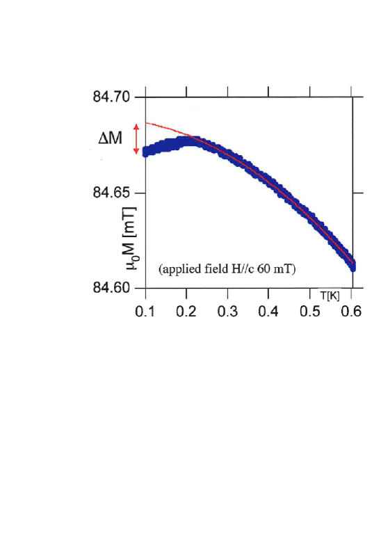
Figure 3: (Color online) The change of static magnetization in URhGe in a constant applied field of 0.06 T Huxley2004 .

The magnetic moment decrease in the ferromagnetic superconducting mixed state is registered experimentally in URhGe Aoki01 and in UCoGe Paulsen2012 ; Hykel2014 . The temperature dependence of magnetization in URhGe is shown in Fig.3.

IV Transition from superconducting to superconducting ferromagnetic state

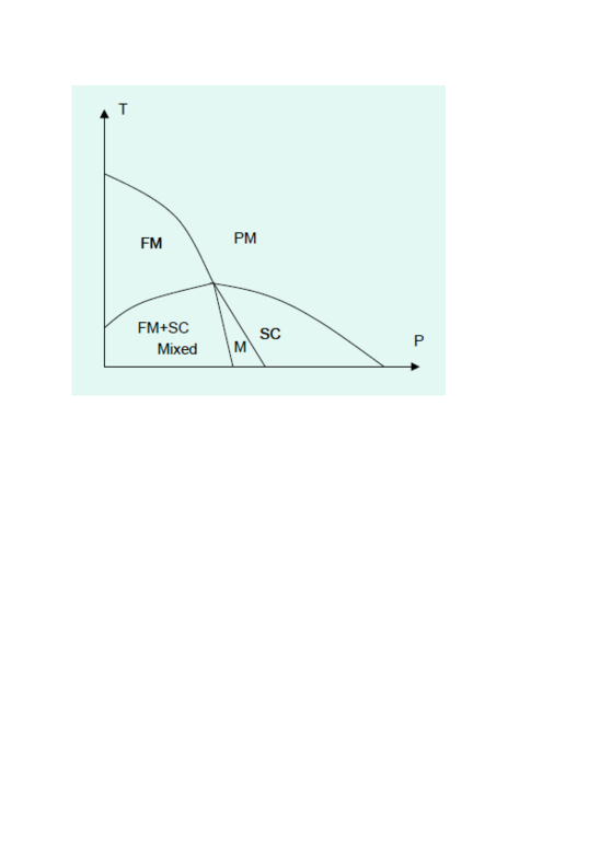
Figure 4: Schematic temperature-pressure phase diagram of UCoGe. Notations FM, SC and PM used for ferromagnetic, superconducting and paramagnetic phases correspondingly. M is the Meissner state divided from the the mixed ferromagnetic superconducting states by the line of $H_{c1}$ Mineev2017 .

In previous chapter we discussed the phase transition from the ferromagnetic state to ferromagnetic superconducting mixed state taking place in all uranium ferromagnets at temperature decrease in zero field (Fig.1) and also in an external field parallel to the spontaneous magnetization. This case the superconducting order parameter forms the vortex lattice where vortices are closely packed together: the distance between them is of the order of the coherence length $\xi(T)$. Another situation is realized in UCoGe (Fig.1c). At pressures larger 1 GPa the Curie temperature falls below the superconducting critical temperature and the phase transition occurs to nonmagnetic superconducting state. The pressure decrease transforms this state into ferromagnetic superconducting state. Theoretically the phase transformation from normal to superconducting state and the subsequent transition to superconducting ferromagnet state in neutral superfluid with triplet pairing have been described in Ref.8,9. There was also predicted Raghu2016 the direct first-order phase transition between the normal and superconducting ferromagnet state. It occurs in some pressures interval when the temperatures of transition to ferromagnetic and superconducting state are closed each other (see Appendix). So long the magnetization is small enough it does not penetrate inside the bulk of material being screened by the surface supercurrents. At pressure decrease the magnetization free superconducting state passes into the ferromagnetic superconducting mixed state. This transformation is complete analog of transition between the Meissner and the mixed superconducting state Mineev2017 (see Fig.4). The ferromagnetic magnetization increasing with pressure decrease penetrates to the superconducting volume in form of quantized vortices. This is happen when it reaches the value of the lower critical field $M_{c1}=H_{c1}/4\pi$ in this material. In the type-II ferromagnetic superconductors $H_{c1}\ll H_{c2}$ and at $M$ slightly above $M_{c1}$ the distance between vortices

$$r_{0}\approx\xi\sqrt{\frac{H_{c2}}{4\pi M_{c1}}}$$ (67)

is large in comparison with coherence length. Thus, it is reasonable to study the field and the order parameter distributions around an isolated vortex.

IV.1 Single vortex

An isolated vortex in an uniaxial metal that I discuss is axially symmetric. It has a phase which changes by $2\pi$ after rotation around its axis directed along the spontaneous magnetization $M_{0}\hat{z}$. When the coefficient $\gamma_{2}=-|\gamma_{2}|$ is negative the phase difference between the superconducting order parameters is absent Mineev2017 and I put it equal to the azimuthal angle $\varphi$ in the cylindrical frame $(r,\varphi,z)$. Thus, I will look for a solution of GL equations (13), (14) in the form

$$\eta_{1}=f_{1}(r)e^{i\varphi},~{}~{}~{}~{}~{}\eta_{2}=f_{2}(r)e^{i\varphi}.$$ (68)

The vector potential has only a $\varphi$-component: ${\bf A}=(0,A_{\varphi},0)$, and the gauge invariant vector potential is

$${\bf Q}=(0,A_{\varphi}-\frac{\hbar c}{2er},0).$$ (69)

The GL equations are

$$(\alpha_{1}+\gamma_{1}B)f_{1}-K_{1}\left[\frac{\partial^{2}}{\partial r^{2}}+\frac{1}{r}\frac{\partial}{\partial r}-\frac{4e^{2}Q^{2}}{\hbar^{2}c^{2}}\right]f_{1}+\gamma_{2}f_{2}+2\beta_{1}f_{1}^{3}+\beta_{2}f_{1}f_{2}^{2}=0,$$ (70)

$$(\alpha_{1}-\gamma_{1}B)f_{2}-K_{2}\left[\frac{\partial^{2}}{\partial r^{2}}+\frac{1}{r}\frac{\partial}{\partial r}-\frac{4e^{2}Q^{2}}{\hbar^{2}c^{2}}\right]f_{2}+\gamma_{2}f_{1}+2\beta_{1}f_{2}^{3}+\beta_{2}f_{2}f_{1}^{2}=0$$ (71)

The field distribution around a single vortex is determined by the Maxwell equation derived from the stationary condition of the GL functional with respect of vector potential

$$curl~{}curl{\bf A}-4\pi curl{\bf M}+4\pi\gamma_{1}curl\hat{z}(f_{1}^{2}-f_{2}^{2})+\frac{2(4\pi e)^{2}}{\pi(\hbar c)^{2}}(K_{1}f_{1}^{2}+K_{2}f_{2}^{2}){\bf Q}=0$$ (72)

For $r\neq 0$ it is

$$curl~{}curl{\bf Q}-4\pi curl{\bf M}+4\pi\gamma_{1}curl\hat{z}(f_{1}^{2}-f_{2}^{2})+\frac{2(4\pi e)^{2}}{\pi(\hbar c)^{2}}(K_{1}f_{1}^{2}+K_{2}f_{2}^{2}){\bf Q}=0$$ (73)

or

$$\frac{\partial}{\partial r}\frac{1}{r}\frac{\partial rQ}{\partial r}-\frac{2(4\pi e)^{2}}{\pi(\hbar c)^{2}}(K_{1}f_{1}^{2}+K_{2}f_{2}^{2}){Q}=4\pi\frac{\partial(M-\gamma_{1}(f_{1}^{2}-f_{2}^{2}))}{\partial r}$$ (74)

The magnetization is determined from the equation

$$2\alpha M+4\beta M^{3}-2D\Delta M-B=0,$$ (75)

obtained by the variation of the functional Eq.(9) in respect to $M$. The induction is $B=curl_{z}{\bf A}$. Thus, omitting the gradient term $D\Delta M$ which can be thrown out by the same reason as in Eq.(40), we come to the equation

$$2\alpha M+4\beta M^{3}=B=\frac{1}{r}\frac{\partial rQ}{\partial r},$$ (76)

which is valid at $r\neq 0$.

The equations (70), (71), (74) and (76) present the full system of equations determining the space distribution of the $f_{1}(r),~{}f_{2}(r),M(r)$, and $Q(r)$ around single vortex in the ferromagnetic superconductor. The solution of this system can be found only numerically. However, a qualitative description is still possible.

The general solution of Eq.(74)

$$Q(r)=Q_{h}(r)+Q_{i}(r)$$ (77)

consists of the sum of a solution of homogeneous equation and a particular solution of the inhomogeneous equation.

At distances larger than the London penetration depth from the vortex axis

$$r>\lambda=\frac{\sqrt{\pi}\hbar c}{4\pi e\sqrt{2(K_{1}f_{10}^{2}+K_{2}f_{20}^{2})}}$$

the functions $f_{1}(r)\approx f_{10},~{}f_{2}(r)\approx f_{20},M(r)\approx M_{0}$ are almost constant and

$$Q_{h}(r)=-\frac{\Phi_{0}}{2\pi\lambda}{\cal K}_{1}\left(\frac{r}{\lambda}\right),$$ (78)

where the function ${\cal K}_{1}(z)$ is the Macdonald function of first order. It decreases exponentially for large $z$:

$${\cal K}_{1}(z)=\sqrt{\frac{2}{\pi z}}\exp(-z).$$

The constant magnetization $M_{0}$ is determined from the Eq.(63) with $B=0$. The corresponding solution of inhomogeneous Eq.(74) is

$$Q_{i}=4\pi\lambda^{2}\frac{\partial(M_{0}-\gamma_{1}(f_{10}^{2}-f_{20}^{2}))}{\partial r}=0.$$ (79)

The induction $B=curl_{z}({\bf Q}_{h}+{\bf Q}_{i})$ is exponentially small. The constants $f_{10},~{}f_{20}$ are found from the equations (70), (71) at $Q(r)=0$.

The solution of equations (70), (71) at the small $r<\xi\approx\sqrt{K_{1,2}/|\alpha_{1}|}$ is $f_{1}\propto r/\xi,~{}~{}~{}f_{2}\propto r/\xi$. The induction $B=curl_{z}({\bf Q}_{h}+{\bf Q}_{i})=B_{0}$, where the constant $B_{0}$ must be found as the limiting value of the numerical solution of equations in intermediate region $\xi<r<\lambda$, $Q=2\pi rM$ and magnetization is determined by equation

$$2\alpha M+4\beta M^{3}=B_{0}.$$ (80)

The crucial difference with vortex solution for ordinary type-II superconductors is the behavior of the order parameters in the intermediate distance interval $\xi<r<\lambda$. Here, all the functions $f_{1}(r),~{}f_{2}(r),~{}M(r),~{}B(r)=curl_{z}{\bf A}$ are gradually changed (see Fig.5).

IV.2 Lower critical field

The free energy of single vortex is the difference between the energy Eq.(9) at stationary vortex solution and the energy without vortex, that is at stationary constant $\eta_{1},~{}\eta_{2},M_{0},B=0$,

$$E_{v}=\int dV\left\{\alpha M^{2}({\bf r})+\beta M^{4}({\bf r})+\alpha_{1}(|\eta_{1}({\bf r})|^{2}+|\eta_{2}({\bf r})|^{2})+\gamma_{1}B({\bf r})(|\eta_{1}({\bf r})|^{2}-|\eta_{2}({\bf r})|^{2})\right.$$

$$+\left.\gamma_{2}(\eta_{1}({\bf r})\eta_{2}^{\star}({\bf r})+\eta_{1}^{\star}({\bf r})\eta_{2}({\bf r}))+\beta_{1}(|\eta_{1}({\bf r})|^{4}+|\eta_{2}({\bf r})|^{4})+\beta_{2}|\eta_{1}({\bf r})|^{2}|\eta_{2}({\bf r})|^{2}\right.$$

$$\left.+K_{1}[(D_{x}\eta_{1}({\bf r}))^{\star}D_{x}\eta_{1}({\bf r})+(D_{y}\eta_{1}({\bf r}))^{\star}D_{y}\eta_{1}({\bf r})]+K_{2}[(D_{x}\eta_{2}({\bf r}))^{\star}D_{x}\eta_{2}({\bf r})+(D_{y}\eta_{2}({\bf r}))^{\star}D_{y}\eta_{2}({\bf r})]+\frac{{\bf B}^{2}}{8\pi}-{\bf B}{\bf M}\right\}$$

$$-\int dV\left\{\alpha M_{0}^{2}+\beta M_{0}^{4}+\alpha_{1}(|\eta_{1}|^{2}+|\eta_{2}|^{2})+\gamma_{2}(\eta_{1}\eta_{2}^{\star}+\eta_{1}^{\star}\eta_{2})+\beta_{1}(|\eta_{1}|^{4}+|\eta_{2}|^{4})+\beta_{2}|\eta_{1}|^{2}|\eta_{2}|^{2}\right\}$$ (81)

The corresponding expression for the conventional single band type-II superconductor is obtained if we put $M=0,\\ \eta_{1}=\eta_{2}$. This case the kinetic energy term contains $K_{1}(4e^{2}/c^{2})Q^{2}|\eta_{1}|^{2}$. Since $Q\propto 1/r$ for $\xi\ll r\ll\lambda$, this gives a logarithmically large contribution at distances $r\sim\lambda$. Because modulus of the vortex order parameter $|\eta_{1}({\bf r})|=|\eta_{1}|=const$ everywhere at $r>\xi$ from the vortex axis the other terms add nothing to the vortex energy. As result the energy of a single-quantum Abrikosov vortex is

$$E_{vA}=\frac{\Phi_{0}^{2}}{(4\pi\lambda)^{2}}\ln\left(\frac{\lambda}{\xi}\right).$$

In ferromagnetic two-band superconductor with triplet pairing the situation is different. In the interval of distances $\xi<r<\lambda$ all the order parameters $f_{1}(r),~{}f_{2}(r),~{}M(r)$ do not coincide with its values in the vortex absence. Hence, the vortex energy does not have the usual logarithmic form. It can be calculated only numerically making use the solution of Eqs.(70), (71), (74) and (76).

The free energy of a unit volume of a superconductor with set of single-quantum vortices is obtained by multiplication of the vortex energy on the density of vortices $n=\langle B\rangle/\Phi_{0}$, where $\langle B\rangle$ is the induction space average. Magnetization begins penetrate in the bulk of superconductor when loss of energy due to vortices appearance will be compensated by gain of the energy due to disappearance of work on pushing out of magnetization from volume of superconductor

$$\frac{\langle B\rangle}{\Phi_{0}}E_{v}-M\langle B\rangle<0.$$ (82)

Thus, in UCoGe, at pressure decrease the magnetization reaches the lower critical value

$$M_{c1}(P,T)=\frac{E_{v}}{\Phi_{0}},$$ (83)

and the transition from the Meissner to the superconducting mixed state occurs. In the presence of external field parallel to the domain magnetization this formula acquires the following form

$$(H+4\pi M)_{c1}=\frac{4\pi}{\Phi_{0}}E_{v}.$$ (84)

V Conclusion

I have developed the theory of type-II superconductivity in two band ferromagnetic metals with triplet pairing. The obtained results near the upper critical field are in qualitative correspondence with the results of classic Abrikosov theory for type-II superconductivity in single band metals with singlet pairing. However, the magnetization decrease below the transition to the superconducting ferromagnetic state is not expressed through the universal ratio known in the Abrikosov theory. The essential distinction also presents the coordinate dependence of the order parameters and the magnetic field around isolated quantized vortex that leads to the different magnitude in vortex line energy in comparison with its value in conventional superconductors.

The theory is applicable to the description of superconducting state arising deeply inside the ferromagnetic state in UGe₂, URhGe, UCoGe. The particular attention is devoted to the transition from the Meissner to the superconducting mixed state specific for UCoGe.

The presented approach can be also applied to the description of type-II superconductivity in two band nonmagnetic metals either with singlet or with triplet pairing.

Appendix A

The direct first order transition from normal to superconducting ferromagnetic state in neutral Fermi liquid has been predicted by Cheung and Raghu Raghu2016 by means the numerical calculations. An attempt to confirm this by analytical treatment undertaken in Ref.9 is incorrect. The proper qualitative argumentation in support of conclusion Ref.8 is as follows. Taking electron charge equal to zero $e=0$ or, in other words, the London penetration depth equal to infinity we come from the present model to the neutral Fermi liquid model discussed in Ref.8,9. This case according to the Eq.(72) the magnetic induction is

$$B=4\pi M-4\pi\gamma_{1}(f_{1}^{2}-f_{2}^{2}).$$ (85)

In absence of gradient terms the free energy density of the ferromagnetic superconductor in respect to the free energy density in the normal state is

$$F=\alpha_{0}(T-T_{c})M^{2}+\beta M^{4}+\alpha_{1}(\eta_{1}^{2}+\eta_{2}^{2})+4\pi\gamma_{1}M(\eta_{1}^{2}-\eta_{2}^{2})-2|\gamma_{2}|\eta_{1}\eta_{2}+\beta_{1}(\eta_{1}^{4}+\eta_{2}^{4})+\beta_{2}\eta_{1}^{2}\eta_{2}^{2}-2\pi[\gamma_{1}(\eta_{1}^{2}-\eta_{2}^{2}]^{2}.$$ (86)

In the normal state $\eta_{1}=\eta_{2}=M=0$ and $F=0$. However, due to the linear in $M$ term $4\pi\gamma_{1}M(\eta_{1}^{2}-\eta_{2}^{2})$ one can find that the state with $F=0$ can be realized also at nonzero order parameter values $\eta_{1}\neq 0,~{}\eta_{2}\neq 0,~{}M\neq 0$. These two states are divided by the phase transition of the first order. Indeed, as this was shown in Ref.8, the first order type transition occurs near the intersection the line $\alpha(T,P)=0$ with the line $\alpha_{1}(T,P)=0$ . The width of pressures interval where the first order transition occurs is in fact negligibly small. This is due to the smallness of $\gamma_{1}$ coefficient already pointed out in the main text (see Eq.(19)). Here,

$$\frac{\gamma_{1}M}{\alpha_{10}}\approx\frac{\mu_{B}M}{\varepsilon_{F}}T_{sc0}\ll T_{sc0},$$ (87)

where $\mu_{B}$ is the Bohr magneton and $\varepsilon_{F}$ is the Fermi energy Book . Thus, the corresponding term is practically insignificant.

In charged Fermi liquid the direct transition from the normal to the superconducting ferromagnetic state will be apparently of the second order because the appearance of a finite magnetization accompanied by work on pushing out of the magnetic induction from the superconducting volume.

Figure 2: (Color online) Schematic upper critical field $H_{c2}(T)$ temperature dependence: for single domain - lower (blue) curve and for multi-domain specimen - upper (red) curve.

Figure 5: Schematic coordinate dependences around an isolated vortex of $f_{1}(r)$ and $f_{2}(r)$ superconducting order parameter amplitudes which grow up linearly at $r<\xi$ and tend to constants at $r>\lambda$. $B(r)$ is the magnetic induction decreasing with distance from the vortex axis and tending to zero at $r>\lambda$.

References

• (1) M.B.Maple, Physica b 215, 110 (1995).
• (2) S. S. Saxena, P. Agarval, K. Ahilan, F. M. Grosche, R. K. W. Hasselwimmer, M. J. Steiner, E. Pugh, I. R. Walker, S. R. Julian, P. Monthoux, G. G. Lonzarich, A. Huxley, I. Sheikin, D. Braithwaite and J. Flouquet, Nature 406, 587 (2000).
• (3) D. Aoki, A. Huxley, E. Ressouche, D. Braithwaite, J. Flouquet, J.-P. Brison, E. Lhotel and C. Paulsen, Nature 413, 613 (2001).
• (4) N. T. Huy, A. Gasparini, D. E. de Nijs, Y. Huang, J. C. P. Klaasse, T. Gortenmulder, A. de Visser, A. Hamann, T. Gorlach, and H. v. Lohneysen, Phys. Rev. Lett. 99, 067006, (2007).
• (5) D. Aoki and J. Flouquet, J. Phys. Soc. Jpn. 83, 061011 (2014).
• (6) V. P. Mineev, Usp. Fizich. Nauk 187, 129 (2017) [ Phys. Usp. 60, 121 (2017)].
• (7) V. P. Mineev, Phys. Rev. B 66, 134504 (2002).
• (8) A. K.C. Cheung and S. Raghu, Phys. Rev. B 93, 134516 (2016).
• (9) V. P. Mineev, Phys. Rev. B 95, 104501 (2017).
• (10) V.H.Dao, S.Burdin, and A.Buzdin, Phys.Rev. 84, 134503 (2011).
• (11) K. Deguchi, E. Osaki, S. Ban, N. Tamura, Y. Simura, T. Sakakibara, I. Satoh, and N. K. Sato, J. Phys. Soc. Jpn. 79, 083708 (2010).
• (12) C. Paulsen, D. J. Hykel, K. Hasselbach, and D. Aoki, Phys. Rev. Lett. 109 237001 (2012).
• (13) D. J. Hykel, C. Paulsen, D. Aoki, J. R. Kirtley, and K. Hasselbach, Phys. Rev. B 90, 184501 (2014).
• (14) A.A.Abrikosov, Zh.Eksp.Teor.Fiz. 32, 1442 (1957) [Sov.Phys.JETP 5, 1174 (1957)].
• (15) E.I.Blount and C.M.Varma, Phys. Rev.Lett. 42, 1079 (1979).
• (16) C.G.Kuper, M.Revzen, and A.Ron, Phys. Rev.Lett. 44, 1545 (1980).
• (17) S.B.Chung, D.F.Agterberg and Eun-A Kim, New Journal og Physics 11, 085004 (2011).
• (18) N.B.Kopnin. J. Low. Temp.Phys. 129, 219 (2002).
• (19) V. P. Mineev and K. V. Samokhin, ”Introduction to Unconventional Superconductivity”, Gordon and Breach Science Publishers, 1999.
• (20) M. E. Zhitomirsky and V.-H. Dao, Phys. Rev. B 69, 054508 (2004).
• (21) F.Hardy, and A.D.Huxley, Phys. Rev. Lett. 94, 247006 (2005).
• (22) A.D.Huxley, CMMP Conference, Warwick 2004.
Refer to caption