Dynamic phase transition of the Blume-Capel model in an oscillating magnetic field

Abstract

We employ numerical simulations and finite-size scaling techniques to investigate the properties of the dynamic phase transition that is encountered in the Blume-Capel model subjected to a periodically oscillating magnetic field. We mainly focus on the study of the two-dimensional system for various values of the crystal-field coupling in the second-order transition regime. Our results indicate that the present non-equilibrium phase transition belongs to the universality class of the equilibrium Ising model and allow us to construct a dynamic phase diagram, in analogy to the equilibrium case, at least for the range of parameters considered. Finally, we present some complementary results for the three-dimensional model, where again the obtained estimates for the critical exponents fall into the universality class of the corresponding three-dimensional equilibrium Ising ferromagnet.

I Introduction

Although our understanding of equilibrium critical phenomena has developed to a point where well-established theories and results are available for a wide variety of systems, far less is known for the physical mechanisms underlying the non-equilibrium phase transitions of many-body interacting systems. In this respect, theoretical but also experimental studies deserve a particular attention in order to provide further insight on the universality and scaling principles of this type of phenomena. We know today that when a ferromagnetic system, below its Curie temperature, is exposed to a time-dependent oscillating magnetic field, it may exhibit a fascinating dynamic magnetic behavior, which cannot be directly obtained via its corresponding equilibrium part Tome . In a typical ferromagnetic system being subjected to an oscillating magnetic field, there occurs a competition between the time scales of the applied field period and the meta-stable lifetime, $\tau$, of the system. When the period of the external field is selected to be smaller than $\tau$, the time-dependent magnetization tends to oscillate around a non-zero value, which corresponds to the dynamically ordered phase. In this region, the time-dependent magnetization is not capable to follow the external field instantaneously. However, for larger values of the period of the external field, the system is given enough time to indeed follow the external field. Hence, in this case the time-dependent magnetization oscillates around its zero value, indicating a dynamically disordered phase. When the period of the external field becomes comparable to $\tau$, a dynamic phase transition takes place between the dynamically ordered and disordered phases.

Up to now, there have been several theoretical Lo ; Zimmer ; Acharyya1 ; Chakrabarti ; Acharyya2 ; Acharyya3 ; Buendia1 ; Buendia2 ; Jang1 ; Jang2 ; Shi ; Punya ; Riego ; Keskin1 ; Keskin2 ; Robb1 ; Deviren ; Yuksel1 ; Yuksel2 ; Vatansever1 and experimental He ; Robb ; Suen ; Berger ; Riego1 studies regarding dynamic phase transitions, as well as the hysteresis properties of different types of magnetic materials. These works indicate that, in addition to the temperature, both the amplitude and the period of the time-dependent magnetic field play a key role in dynamical critical phenomena. On the other hand and to the best of our knowledge, there exist only few studies focusing on the critical exponents and universality aspects of spin models driven by a time-dependent oscillating magnetic field Sides1 ; Sides2 ; Korniss ; Buendia3 ; Park ; Tauscher ; Vatansever2 . In particular, by means of Monte Carlo simulations and finite-size scaling analysis, it has been suggested that the critical exponents of the two-dimensional (2D) kinetic Ising model are compatible to those of the corresponding 2D equilibrium Ising model Korniss ; Sides1 ; Sides2 . In another relevant work Buendia3 , Buendía and Rikvold used soft Glauber dynamics to estimate the critical exponents of the same system, providing strong evidence that the characteristics of the phase transition are universal with respect to the choice of the stochastic dynamics. The above results have been corroborated by a numerical study of the triangular-lattice Ising model Vatansever2 , where the obtained critical exponents were found to be consistent within errors to those of the equilibrium Ising counterpart. Furthermore, the universality features of the 3D kinetic Ising model have been clarified by Park and Pleimling Park : the critical exponents of 3D kinetic Ising model are in good agreement to those of the corresponding equilibrium 3D case. Last but not least, the role of surfaces at non-equilibrium phase transitions has been elucidated in Ref. Park2 where the non-equilibrium surface exponents were found not to coincide with those of the equilibrium critical surface and even more recently the fluctuations in a square-lattice ferromagnetic model driven by a slowly oscillating field with a constant bias have been studied in Ref. Buendia4 . This latter work, provided us with the ubiquitous reminder that the equivalence of the dynamic phase transition to an equilibrium phase transition is limited to the critical region near the critical period and zero bias.

It is evident from the above discussion that most of the numerical work performed to clarify the universality classes of dynamic phase transitions has been devoted to the kinetic spin-$1/2$ Ising type of models. Still, there is another suitable candidate model where the above predictions may be tested: the so-called Blume-Capel model Capel ; Blume . The Blume-Capel model is defined by a spin-1 Ising Hamiltonian with a single-ion uniaxial crystal-field anisotropy (or simpler crystal-field coupling) $\Delta$ Capel ; Blume [see also Eq. (1) below]. The fact that this model has been very widely studied in statistical and condensed-matter physics is explained not only by its relative simplicity and the fundamental theoretical interest arising from the richness of its phase diagram, but also by a number of different physical realizations of variants of the model Lawrie ; Selke . From the theoretical point of view, in order to have a better understanding of the equilibrium phase transition characteristics, the model and its variants have been intensively studied by making use of different methods, such as renormalization-group calculations Berker1 ; Branco ; Snowman , Monte Carlo simulations Jain ; Falicov ; Silva ; Malakis1 ; Malakis2 ; Malakis3 ; Fytas1 ; Kwak ; Zierenberg , and mean-field theory approaches Boccara ; Hoston ; Zahraouy .

Despite intensive investigations devoted to the determination of the time-dependent magnetic-field effects on the dynamic phase transition nature of the spin-1 Blume-Capel model Buendia1 ; Keskin1 ; Keskin2 ; Deviren ; ShiWei ; Acharyya4 , critical exponents and universality properties of the model have not been elucidated. To fill this gap, we present in this paper the first study of universality of the spin-1 square-lattice Blume-Capel model in the neighborhood of a dynamic phase transition under the presence of a time-dependent magnetic field. The aim of our study is threefold: Firstly, we would like to check how the critical exponents of the kinetic spin-1 Blume-Capel model, estimated at various values of $\Delta$ in the second-order transition regime, compare to those of the corresponding equilibrium Ising model. Secondly, we target at constructing a dynamic phase diagram in the related plane for the range of $\Delta$-values considered. In a nutshell, our results indicate that the dynamic phase transition of the present kinetic system belongs to the universality class of the equilibrium Ising model. Some complementary results obtained for the 3D version of this spin-1 kinetic model, presented at the end of this paper, provide additional support in favor of this claim. Furthermore, the obtained dynamic phase diagram is found to be qualitatively similar to the equilibrium phase diagram constructed in the crystal-field – temperature plane Silva ; Malakis2 ; Zierenberg . Last but not least, the data given in this study qualitatively support the previously published studies, where general dynamic phase transition features of the same system have been investigated via mean-field Keskin1 ; Keskin2 and effective-field Deviren theory treatments.

The outline of the remainder parts of the paper is as follows: In Sec. II we introduce the model and the details our simulation protocol. In Sec. III we define the relevant observables that will facilitate our finite-size scaling analysis for the characterization of the universality principles of this dynamic phase transition. The numerical results and discussion for the 2D and 3D model are presented in Secs. IV and Sec. V, respectively. Finally, Sec. VI contains a summary of our conclusions.

II Model and Simulation Details

We consider the square-lattice Blume-Capel model under the existence of a time-dependent oscillating magnetic field. The Hamiltonian of the system reads as

$$\mathcal{H}=-J\sum_{\langle xy\rangle}\sigma_{x}\sigma_{y}+\Delta\sum_{x}\sigma_{x}^{2}-h(t)\sum_{x}\sigma_{x},$$ (1)

where the spin variable $\sigma_{x}$ takes on the values $-1$, $0$, or $+1$, $\langle xy\rangle$ indicates summation over nearest neighbors, and $J>0$ is the ferromagnetic exchange interaction. $\Delta$ denotes the crystal-field coupling and controls the density of vacancies ($\sigma_{x}=0$). For $\Delta\rightarrow-\infty$ vacancies are suppressed and the model becomes equivalent to the Ising model. The term $h(t)$ corresponds to a spatially uniform periodically oscillating magnetic field, and, following the prescription of Refs. Korniss ; Buendia3 ; Park , we assume that all lattice sites are exposed to a square-wave magnetic field with amplitude $h_{0}$ and half period $t_{1/2}$.

The phase diagram of the equilibrium Blume-Capel model in the crystal-field – temperature plane consists of a boundary that separates the ferromagnetic from the paramagnetic phase. The ferromagnetic phase is characterized by an ordered alignment of $\pm 1$ spins. The paramagnetic phase, on the other hand, can be either a completely disordered arrangement at high temperature or a $\pm 1$-spin gas in a $0$-spin dominated environment for low temperatures and high crystal fields. At high temperatures and low crystal fields, the ferromagnetic-paramagnetic transition is a continuous phase transition in the Ising universality class, whereas at low temperatures and high crystal fields the transition is of first-order character Capel ; Blume . The model is thus a classic and paradigmatic example of a system with a tricritical point $[\Delta_{\rm t},T_{\rm t}]$ Lawrie , where the two segments of the phase boundary meet. A most recent reproduction of the phase diagram of the model can be found in Ref. Zierenberg , and an accurate estimation of the location of the tricritical point has been given in Ref. Kwak : $[\Delta_{\rm t},T_{\rm t}]=[1.9660(1),0.6080(1)]$. However, for the needs of the current work we restricted our analysis in the second-order transition regime of the model $\Delta<\Delta_{\rm t}$. In particular, we studied the system at the following crystal-field values: $\Delta=0$, $0.5$, $1$, $1.5$, and $\Delta=1.75$.

In numerical grounds, we performed Monte Carlo simulations on square lattices with periodic boundary conditions using the single-site update Metropolis algorithm Metropolis ; Binder ; Newman . This approach, together with the alternative option of stochastic Glauber dynamics Glauber:63 , consists the standard recipe in kinetic Monte Carlo simulations, as was also noted in Ref. Buendia3 . In fact, very recently, the surface phase diagram of the 3D kinetic Ising model in an oscillating magnetic field has been studied within the framework of both Glauber and Metropolis dynamics and it was been shown that the results remain qualitatively unchanged when using different single-spin flip dynamics Tauscher .

In our simulations, $N=L\times L$ defines the total number of spins and $L$ the linear dimension of the lattice, taking values within the range $L=32-256$. For each pair of ($L$, $\Delta$)-parameters we performed several independent long runs, tailored for the value of $\Delta$ under study, using the following protocol: the first $10^{3}$ periods of the external field have been discarded during the thermalization process and numerical data were collected and analyzed during the following $10^{4}$ periods of the field. We note that the time unit in our simulations is one Monte Carlo step per site (MCSS) and that error bars have been estimated using the jackknife method Newman . To set the temperature scale we fixed units by choosing $J=1$ and $k_{\rm B}=1$, where $k_{\rm B}$ is the Boltzmann constant. Appropriate choices of the magnetic-field strength, $h_{0}=0.2$, and the temperature, $T(\Delta)=0.8T_{\rm c}(\Delta)$, ensured that the system is in the multi-droplet regime Park . Here, $T_{\rm c}(\Delta)$ denotes the set of critical temperatures of the equilibrium square-lattice Blume-Capel model, as estimated in Ref. Malakis2 and also given in Tab. 1 below. Finally, for the application of finite-size scaling on the numerical data, we restricted ourselves to data with $L\geq L_{\rm min}$. As usual, to determine an acceptable $L_{\rm min}$ we employed the standard $\chi^{2}$-test of goodness of fit Press . Specifically, the $p$-value of our $\chi^{2}$-test is the probability of finding an $\chi^{2}$ value which is even larger than the one actually found from our data. We considered a fit as being fair only if $10\%<p<90\%$.

A similar prescription was also followed for the study of the 3D version of the model and the details of this implementation will be given later on, in the beginning of Sec. V.

III Observables

In order to determine the universality aspects of the kinetic Blume-Capel model, we shall consider the half-period dependencies of various thermodynamic observables. The main quantity of interest is the period-averaged magnetization

$$Q=\frac{1}{2t_{1/2}}\oint M(t)dt,$$ (2)

where the integration is performed over one cycle of the oscillating field. Given that for finite systems in the dynamically ordered phase the probability density of $Q$ becomes bimodal, one has to measure the average norm of $Q$ in order to capture symmetry breaking, so that $\langle|Q|\rangle$ defines the dynamic order parameter of the system. In the above Eq. (2), $M(t)$ is the time-dependent magnetization per site

$$M(t)=\frac{1}{N}\sum_{x=1}^{N}\sigma_{x}(t).$$ (3)

To characterize and quantify the transition using finite-size scaling arguments we must also define quantities analogous to the susceptibility in equilibrium systems. The scaled variance of the dynamic order parameter

$$\chi_{L}^{Q}=N\left[\langle Q^{2}\rangle_{L}-\langle|Q|\rangle^{2}_{L}\right],$$ (4)

has been suggested as a proxy for the non-equilibrium susceptibility, also theoretically justified via fluctuation-dissipation relations Robb1 . Similarly, one may also measure the scaled variance of the period-averaged energy

$$\chi_{L}^{E}=N\left[\langle E^{2}\rangle_{L}-\langle E\rangle^{2}_{L}\right],$$ (5)

so that $\chi_{L}^{E}$ can be considered as the relevant heat capacity of the dynamic system. Here $E$ denotes the cycle-averaged energy corresponding to the cooperative part of the Hamiltonian (1)

$$E=\frac{1}{2t_{1/2}N}\oint\left[-J\sum_{\langle xy\rangle}\sigma_{x}\sigma_{y}+\Delta\sum_{x}\sigma_{x}^{2}\right]dt.$$ (6)

A few comments are in order at this point with respect to the use of the above Eqs. (5) and (6), where we focus only on the cooperative part of the energy in order to calculate the time-averaged energy over a full cycle of the external field and its corresponding variance. Conceptually, the role of the time-averaged energy originating from an oscillating magnetic field (namely, the time-dependent Zeeman term) can be better understood with the help of the dynamic correlation function. In spin systems driven by a time-dependent external field there may be some dynamic correlations between the time-dependent magnetic field and the time-dependent magnetization, which strongly depend on the chosen temperature, including other parameters as well. In order to explain this point in detail, let us define the dynamic correlation function $G=\langle M(t)h(t)\rangle-\langle M(t)\rangle\langle h(t)\rangle$, where $\langle\cdots\rangle$ denotes the time-average over a full cycle of the external field Acharyya95 . Since $\langle h(t)\rangle=0$, we are allowed to simplify as $G=\langle M(t)h(t)\rangle$. We know that in the relatively strong ferromagnetic phase the spin-spin interactions are dominant against the field energy. Therefore, the spins do not tend to respond to the varying magnetic field for fixed system parameters. In other words, the corresponding dynamic correlation function is almost zero in this region. In the regions, except from the strongly ferromagnetic and paramagnetic phases, the relevant term may have a non-zero value, however the energy term coming from this type of a behavior does not effect the true dynamic phase transition point Acharyya2 .

Finally, with the help of the dynamic order parameter $Q$ we may define the corresponding fourth-order Binder cumulant Sides1 ; Sides2

$$U_{L}=1-\frac{\langle|Q|^{4}\rangle_{L}}{3\langle|Q|^{2}\rangle_{L}^{2}},$$ (7)

which provides us with an alternative estimation of the critical point, giving at the same time a flavor of universality at its intersection point Binder81 .

IV Results and discussion

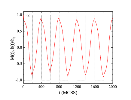
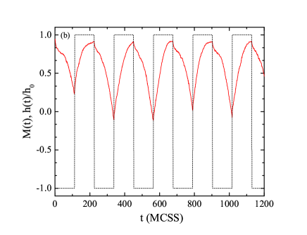
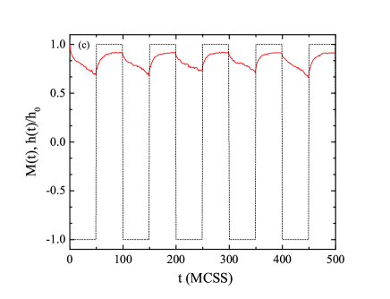
Figure 1: (Color online) Time series of the magnetization (red solid curves) of the $\Delta=1$ kinetic spin-1 Blume-Capel model under the presence of a square-wave magnetic field (black dashed lines) for $L=128$ and three values of the half period of the external field: (a) $t_{1/2}=200$ MCSS, corresponding to a dynamically disordered phase, (b) $t_{1/2}=113$ MCSS, close to the dynamic phase transition, and (c) $t_{1/2}=50$ MCSS, corresponding to a dynamically ordered phase. Note that for the sake of clarity the ratio $h(t)/h_{0}$ is displayed.

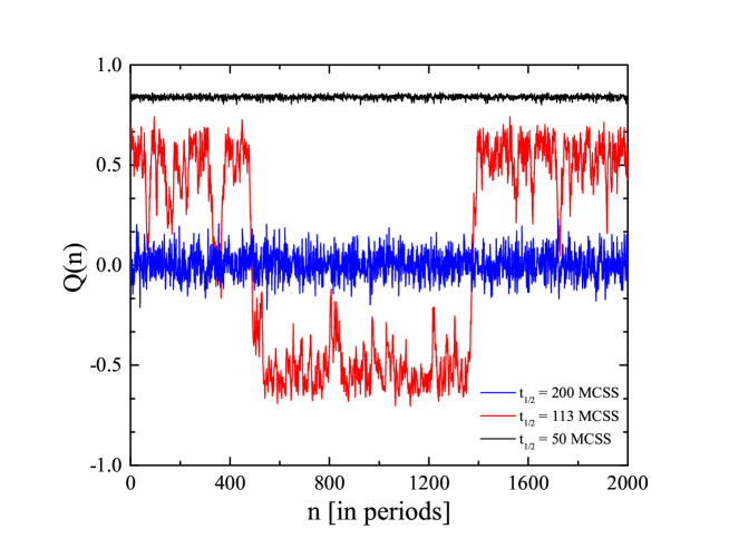
Figure 2: (Color online) Period dependencies of the dynamic order parameter of the $\Delta=1$ kinetic spin-1 Blume-Capel model for $L=128$. Results are shown for three characteristic cases of the half period of the external field: $t_{1/2}=200$ MCSS (blue line), $t_{1/2}=113$ MCSS (red line), and $t_{1/2}=50$ MCSS (black line). The strongly fluctuating trace (red line) corresponds to the vicinity of the dynamic phase transition, given that $t_{1/2}\approx t_{1/2}^{\rm c}=112.3\pm 1.3$, as will be shown below.

It may be useful at this point to shortly describe the mechanism underlying the dynamical ordering that takes place in kinetic ferromagnets, as exemplified in Figs. 1 and 2 for the case of the $\Delta=1$ Blume-Capel model and a system size of $L=128$. In particular, Fig. 1 presents the time evolution of the magnetization and Fig. 2 the period dependencies of the dynamic order parameter $Q$. Several comments are in order at this point: For slowly varying fields, Fig. 1(a), the magnetization follows the field, switching every half period. In this region, as expected, $Q\approx 0$, as also shown by the blue line in Fig. 2. On the other hand, for rapidly varying fields, Fig. 1(c), the magnetization does not have enough time to switch during a single half period and remains nearly constant for many successive field cycles, as also illustrated by the black line in Fig. 2. In other words, whereas in the dynamically disordered phase the ferromagnet is able to reverse its magnetization before the field changes again, in the dynamically ordered phase this is not possible and therefore the time-dependent magnetization oscillates around a finite value. The competition between the magnetic field and the meta-stable state is captured by the half-period parameter $t_{1/2}$ (or by the normalized parameter $\Theta=t_{1/2}/\tau$, with $\tau$ being the meta-stable lifetime Park ). Obviously, $t_{1/2}$ plays the role of the temperature in the corresponding equilibrium system. Now, the transition between the two regimes is characterized by strong fluctuations in $Q$, see panel (b) in Fig. 1 and the evolution of the red line in Fig. 2. This behavior is indicative of a dynamic phase transition and occurs for values of the half period close to the critical one $t_{1/2}^{\rm c}$ (otherwise stated when $t_{1/2}\approx\tau$, so that $\Theta\approx 1$). Of course, since the value $t_{1/2}=113$ MCSS used for this illustration is slightly above $t^{\rm c}_{1/2}$ for the case $\Delta=1$, see Tab. 1, the observed behavior includes as well some non-vanishing finite-size effects.

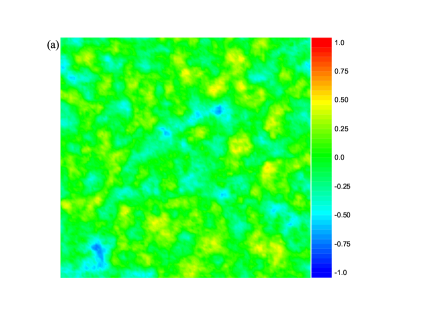
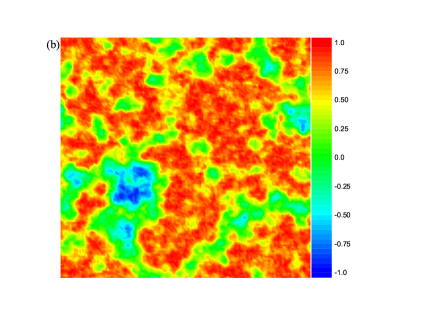
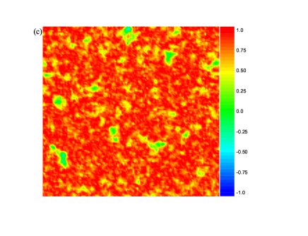
Figure 3: (Color online) Configurations of the local dynamic order parameter $\{Q_{x}\}$ of the $\Delta=1.75$ kinetic spin-1 Blume-Capel model for $L=128$. The “snapshots” of $\{Q_{x}\}$ for each regime are the set of local period-averaged spins during some representative period. Three panels are shown: (a) $t_{1/2}=100$ MCSS $>t_{1/2}^{\rm c}$ - dynamically disordered phase, (b) $t_{1/2}=43$ MCSS $\approx t_{1/2}^{\rm c}$ - near the dynamic phase transition, and (c) $t_{1/2}=20$ MCSS $<t_{1/2}^{\rm c}$ - dynamically ordered phase.

To illustrate the spatial aspects of the transition scenario described above in Figs. 1 and 2, we also show configurations of the local order parameter $\{Q_{x}\}$ in Fig. 3 for the case of the $\Delta=1.75$ Blume-Capel model and a system of linear size $L=128$. When the period of the external field is selected to be bigger than the relaxation time of the system, above $t_{1/2}^{\rm c}$, see panel (a), the system follows the field in every half period, with some phase lag, and $Q_{x}\approx 0$ at all sites $x$. In other words the system lies in the dynamically disordered phase. On the other hand, below $t_{1/2}^{\rm c}$, see panel (c), the majority of spins spend most of their time in the $+1$ state, i.e., in the meta-stable phase during the first half period, and in the stable equilibrium phase during the second half period, except for equilibrium fluctuations. Thus most of the $Q_{x}\approx+1$. The system is now in the dynamically ordered phase. Near $t_{1/2}^{\rm c}$ and the expected dynamic phase transition, there are large clusters of both $+1$ and $-1$ states, within a sea of $0$-state spins, as clearly illustrated in panel (b) of Fig. 3.

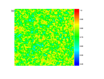
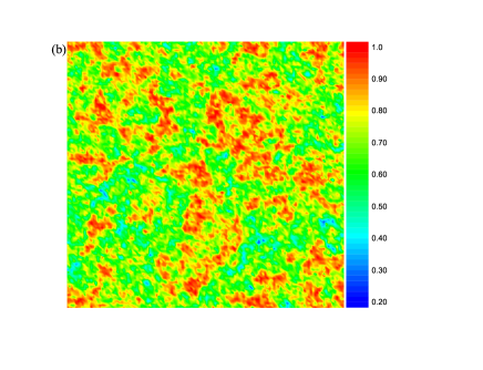
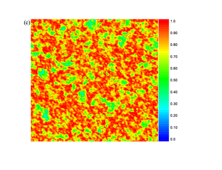
Figure 4: (Color online) In full analogy to Fig. 3 we show snapshots of the period-averaged quadrupole moment conjugate to the crystal-field coupling $\Delta$. The simulation parameters are exactly the same as those used in Fig. 3 for all three panels (a) - (c).

However, the value of the local order parameter $\{Q_{x}\}$ does not distinguish between random distributions of $\sigma_{x}=\pm 1$ and and regions of $\sigma_{x}=0$. To bring out this distinction, we present in Fig. 4 similar snapshots of the dynamic quadrupole moment over a full cycle of the external field, $O=\frac{1}{2t_{1/2}}\oint q(t)dt$, where $q(t)=\frac{1}{N}\sum_{x=1}^{N}\sigma_{x}^{2}$. The simulation parameters are exactly the same to those used in Fig. 3 for all three panels (a) - (c). Of course, the dynamic quadrupole moment is always one for the kinetic spin-1/2 Ising model, because $\sigma_{x}=\pm 1$ in this case. In the spin-1 Blume-Capel model the density of the ($\sigma_{x}=0$) vacancies is controlled by the the crystal-field coupling $\Delta$ and, thus, the value of the dynamic quadrupole moment changes depending on $\Delta$. When the value of $\Delta$ increases, starting from its Ising limit $(\Delta\rightarrow-\infty)$, the number of vacancies increases as well in the system, so that the dynamic quadrupole moment tends to decrease from its maximum value. In Fig. 4, except from the regions with red color indicating the $+1$ state, the regions enclosed by finite values exemplify the role played by the the crystal-field coupling on the system.

To further explore the nature of the dynamic phase transition, we performed a finite-size scaling analysis of the simulation data obtained for various values of the crystal-field coupling $\Delta$, as outlined above. Previous studies in the field indicated that although scaling laws and finite-size scaling are tools that have been designed for the study of equilibrium phase transitions, they can be successfully applied as well to far from equilibrium systems, like the current kinetic spin-1 Blume-Capel model Sides1 ; Sides2 ; Korniss ; Buendia3 ; Park .

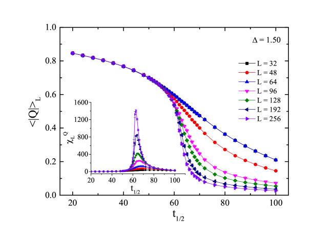
Figure 5: (Color online) Half-period dependency of the dynamic order parameter of the kinetic spin-1 $\Delta=1.5$ Blume-Capel model for a wide range of system sizes studied. The inset represents the corresponding half-period dependency of the corresponding dynamic susceptibility $\chi_{L}^{Q}$.

As an illustrative example for the case $\Delta=1.5$, we present in Fig. 5 the finite-size behavior of the dynamic order parameter (main panel) and the corresponding dynamic susceptibility (inset) for a wide range of system sizes studied. The main panel clearly shows that this dynamic order parameter goes from a finite value to zero values at the half period increases, showing a sharp change around the value of the half period that can be mapped to the corresponding peak in the plot of the dynamic susceptibility. The height and the location of the maximum in $\chi_{L}^{Q}$ change with system size and we may define as suitable pseudo-critical half periods these point locations, denoted hereafter as $t_{1/2}^{\ast}$. The corresponding maxima may be similarly defined as $(\chi^{Q}_{L})^{\ast}$. Moreover, the absence of finite-size effects below the critical point is a clear signature of a divergent length scale. Of course, similar plots may be prepared for all the other values of $\Delta$ studied, providing us with suitable pseudo-critical points and susceptibility maxima that will allow us to perform finite-size scaling.

Table 1: Summary of estimates for the critical half period $t_{1/2}^{\rm c}$, the critical exponent $\nu$, and the magnetic exponent ratio $\gamma/\nu$ of the spin-1 kinetic Blume-Capel model for various values of the crystal-field coupling $\Delta$, as illustrated. The second column lists the critical temperatures of the equilibrium Blume-Capel model, as estimated in Ref. Malakis2 .

$\Delta$	$T_{\rm c}$ Malakis2	$t_{1/2}^{\rm c}$	$\nu$	$\gamma/\nu$
0.00	$1.693(3)$	$206.4\pm 1.2$	1.05(8)	1.74(3)
0.50	$1.564(3)$	$166.6\pm 1.1$	1.01(7)	1.75(1)
1.00	$1.398(2)$	$112.3\pm 1.3$	1.03(9)	1.75(2)
1.50	$1.151(1)$	$61.0\pm 0.3$	0.98(6)	1.76(1)
1.75	$0.958(1)$	$43.1\pm 0.2$	1.02(6)	1.76(2)

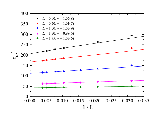
Figure 6: (Color online) Estimation of the critical half period $t_{1/2}^{\rm c}$ and the correlation-length’s exponent $\nu$ of the kinetic spin-1 Blume-Capel model for all values of $\Delta$ considered. The solid lines are fits of form (8).

The shift behavior of the peak locations $t_{1/2}^{\ast}$ is plotted in Fig. 6 as a function of $1/L$ for all the values of the crystal-field coupling considered. The solid lines are fits of the usual shift form Fisher ; Privman ; Binder92

$$t_{1/2}^{\ast}=t_{1/2}^{\rm c}+bL^{-1/\nu},$$ (8)

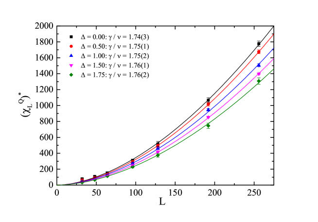
Figure 7: (Color online) Finite-size scaling analysis of the maxima $(\chi_{L}^{Q})^{\ast}$ of the kinetic spin-1 Blume-Capel model for all values of $\Delta$ considered. The solid lines are fits of the form (9).

where $t_{1/2}^{\rm c}$ defines the critical half period of the system and is a function of $\Delta$ and $\nu$ is the critical exponent of the correlation length. The obtained values for the critical half period are given at the third column of Tab. 1. The relevant values for the critical exponent $\nu$ are given in the panel of Fig. 6 but are also listed in the fourth column Tab. 1. These values suggest that the critical exponent $\nu$ of the kinetic Blume-Capel model is compatible, up to a very good accuracy, to the value $\nu=1$ of the 2D equilibrium Ising model, thus providing a first strong element of universality. Subsequently, in Fig. 7 we present the finite-size scaling analysis behavior of the peaks of the dynamic susceptibility and the solid lines are fits of the form Ferrenberg

$$(\chi^{Q}_{L})^{\ast}\sim L^{\gamma/\nu}.$$ (9)

The results for the magnetic exponent ratio $\gamma/\nu$ are given in the panel and also in the fifth column of Tab. 1. Again, these values for all $\Delta$-cases studied in the present work are in good agreement with the expected Ising value $\gamma/\nu=1.75$, reinforcing the scenario of universality for the kinetic Blume-Capel model.

In addition to $\gamma/\nu$, further evidence may be provided via the alternative magnetic exponent ratio, namely $\beta/\nu$, obtained from the scaling behavior of the dynamic order parameter at the critical point via

$$(\langle|Q|\rangle_{L})^{\ast}\sim L^{-\beta/\nu}.$$ (10)

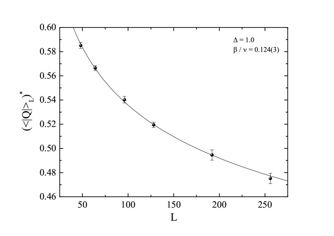
Figure 8: Finite-size scaling analysis of the dynamic order parameter estimated at the critical half period, $(\langle|Q|\rangle_{L})^{\ast}$, of the 2D kinetic spin-1 Blume-Capel model at $\Delta=1$. The solid line is a power-law fit of the form (10).

One characteristic example of this expected scaling behavior for the kinetic spin-1 Blume-Capel model is shown in Fig. 8 for $\Delta=1$. A power-law fit of the form (10) gives an estimate $0.124(3)$ for $\beta/\nu$, in good agreement with the Ising value $1/8=0.125$. Let us note here that similar results have been obtained in our fitting attempts for all the other $\Delta$-values studied in this work.

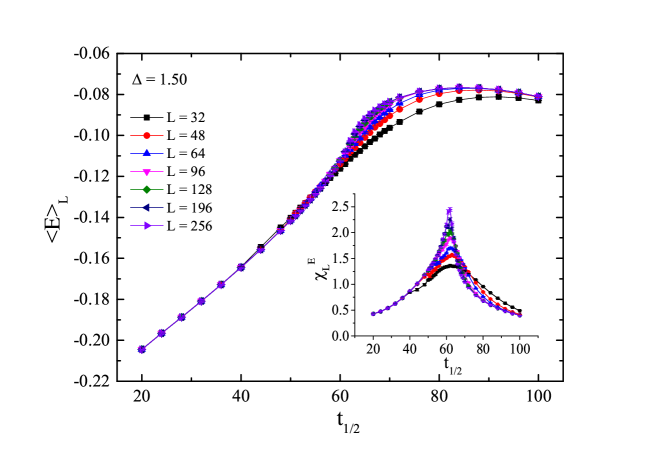
Figure 9: (Color online) Half-period dependency of the energy of the kinetic spin-1 $\Delta=1.5$ Blume-Capel model for a wide range of system sizes studied. The inset illustrates the half-period dependency of the corresponding heat capacity $\chi_{L}^{E}$.

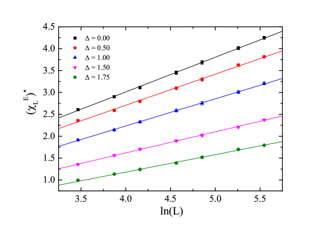
Figure 10: (Color online) Illustration of the logarithmic scaling behavior of the maxima of the heat capacity, $(\chi_{L}^{E})^{\ast}$, for all values of $\Delta$ considered in this work. The solid lines are fits of the form (11).

As mentioned in Sec. III, we also measured the energy and its corresponding scaled variance, the heat capacity (5). Both quantities are shown in the main panel and the corresponding inset of Fig. 9, respectively. Ideally, we would like to observe the logarithmic scaling behavior of the maxima of the heat capacity $(\chi_{L}^{E})^{\ast}$. Indeed, as it is shown in Fig. 10, the data for the maxima of the heat capacity show a clear logarithmic divergence of the form Ferdinand

$$(\chi^{E}_{L})^{\ast}\propto c_{1}+c_{2}\ln{(L)},$$ (11)

as expected for a 2D Ising ferromagnet.

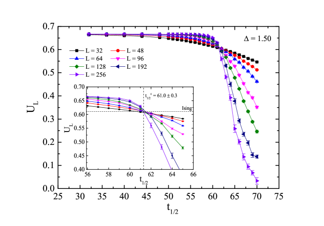
Figure 11: (Color online) Half-period dependency of the fourth-order Binder cumulant $U_{L}$ of the kinetic spin-1 $\Delta=1.5$ Blume-Capel model for a wide range of system sizes studied. The inset displays an enhancement of the intersection area.

A final verification of the equilibrium Ising universality class comes form the study of the Binder cumulant, as defined above for the case of the dynamic order parameter, see Eq. (7). In Fig. 11 we plot the fourth-order cumulant $U_{L}$ for the case $\Delta=1.5$ for the various system sizes considered in this work. The inset is a mere enlargement of the intersection area. The vertical dashed line marks the critical half-period value of the system $t_{1/2}^{\rm c}=61.0\pm 0.3$, as estimated in Fig. 6, and the horizontal dotted line marks the universal value $U^{\ast}=0.6106924(16)$ of the 2D equilibrium Ising model Salas , which is consistent to the crossing point of our numerical data. Certainly, the crossing point is expected to depend on the lattice size $L$ (as it also shown in the figure) and the term universal is valid for given lattice shapes, boundary conditions, and isotropic interactions. For a detailed discussion on this topic we refer the reader to Refs. Selke_2 ; Selke_3 . Still, the scope of the current Fig. 11 is to show qualitatively another instance of the Ising universality. Similar plots and conclusions hold also for the other values of $\Delta$ studied, but are omitted for brevity. As a note, we remind the reader that an alternative way to estimate the critical exponent $\nu$ comes from the scaling behavior of the derivative of the Binder cumulant at the corresponding crossing points, via $\left(\partial U_{L}/\partial t_{1/2}\right)\propto L^{1/\nu}$, an approach that demands quite accurate data at the area of the crossing points for a safe estimation of derivatives Binder .

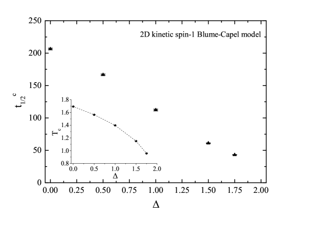
Figure 12: Dynamic $\Delta-t_{1/2}^{\rm c}$ phase boundary of the kinetic spin-1 square-lattice Blume-Capel model. For the sake of completeness we provide in the inset a part of the phase diagram of the equilibrium counterpart in the $(\Delta-T_{\rm c})$ plane using the results of Ref. Malakis2 that were used in the present work. The dotted line is a simple guide to the eye.

We complete our analysis on the 2D model, by presenting in Fig. 12 an illustrative formulation of a dynamic phase diagram for the kinetic spin-1 Blume-Capel model at the $(\Delta-t_{1/2}^{\rm c})$ plane, using the values for the critical half period shown in Tab. 1. We also include a complementary inset with the corresponding equilibrium counterpart in the $(\Delta-T_{\rm c})$ plane using the results of Ref. Malakis2 for the regime of continuous transitions. As it can be seen from the main panel of Fig. 12, the values of $t_{1/2}^{\rm c}$ decrease almost linearly with increasing $\Delta$. We are not currently sure if this is due to the particular selection of the chosen temperatures, $0.8T_{\rm c}(\Delta)$, or it may be a general result for any temperature well below $T_{\rm c}$. Further simulations are needed to clarify this point, that are however out of the scope of the current study.

V On the dynamic phase transition of the 3D Blume-Capel model

In this Section we present some complementary results on the dynamic phase transition of the kinetic spin-1 3D Blume-Capel model, as defined above in Eq. (1), but with the spins living on the simple cubic lattice. In this case $N=L\times L\times L$, where $L\in\{8,16,24,32,48,64\}$. The analysis below is presented for a single value of the crystal-field coupling in the second-order transition regime of the phase diagram, namely for $\Delta=0.655$. For this value of $\Delta$, the critical temperature of the model has been very accurately determined by Hasenbusch to be $T_{\rm c}=2.579169$ Hasenbusch . Our Monte Carlo simulations followed the protocol defined above in Sec. II for the case of the square-lattice model, using now $h_{0}=0.6$ and $T=0.8T_{\rm c}$ as appropriate choices for the magnetic-field strength and the temperature, respectively.

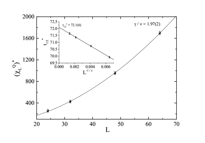
Figure 13: Finite-size scaling analysis of the maxima $(\chi_{L}^{Q})^{\ast}$ (main panel) and shift behavior of the corresponding pseudo-critical half periods $t_{1/2}^{\ast}$ (inset) of the 3D kinetic spin-1 Blume-Capel model.

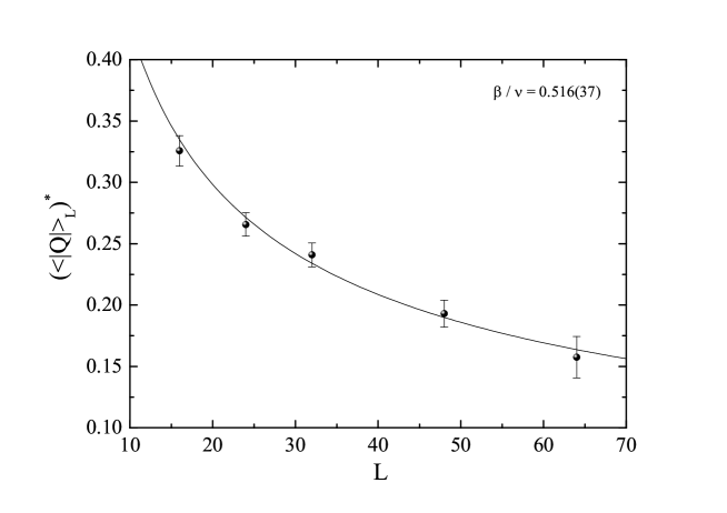
Figure 14: Finite-size scaling analysis of the dynamic order parameter estimated at the critical half period, $(\langle|Q|\rangle_{L})^{\ast}$, of the 3D kinetic spin-1 Blume-Capel model. The solid line is a power-law fit of the form (10).

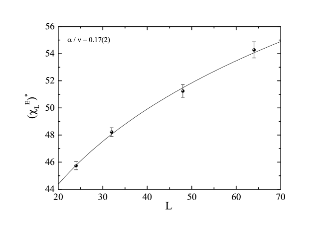
Figure 15: Finite-size scaling analysis of the maxima $(\chi_{L}^{E})^{\ast}$ of the 3D kinetic spin-1 Blume-Capel model The solid line is a power-law fit of the form (12).

We summarize our results in Figs. 13 - 15 below. In particular, in the main panel of Fig. 13 we present the finite-size scaling behavior of the maxima $(\chi_{L}^{Q})^{\ast}$. The solid line in is a fit of the form (9) providing us with the estimate $\gamma/\nu=1.97(2)$ which is in very good agreement to the Ising value $1.96370(2)$ of the equilibrium 3D Ising ferromagnet Kos . In the corresponding inset we illustrate the shift behavior of the pseudo-critical half periods $t_{1/2}^{\ast}$ as a function of $L^{-1/\nu}$, where $\nu$ has been fixed to the Ising value $0.629971$ Kos . The numerical data are well described by a linear extrapolation to the $L\rightarrow\infty$ limit, see also Eq. (8), indicating that the critical exponent $\nu$ of the kinetic version of the 3D Blume-Capel model shares the value of its equilibrium counterpart. The critical half period is also estimated to be $t_{1/2}^{\rm c}=72.1\pm 0.6$ for the particular case of $\Delta$ studied here, as also indicated in the inset.

Figure 14 illustrates the scaling behavior of the dynamic order parameter of the 3D kinetic spin-1 Blume-Capel model at the above estimated critical half period, $(\langle|Q|\rangle_{L})^{\ast}$. Similarly to the 2D model, the solid line is a power-law fit of the form (10), providing the estimate $\beta/\nu=0.516(37)$ for the magnetic exponent ratio that should be compared to the value $0.518149(6)$ of the 3D Ising model Kos . Again, the agreement is beyond any (numerical) doubt.

Finally we discuss the scaling behavior of the heat capacity (5). In Fig. 15 we present the size evolution of the maxima of the heat capacity $(\chi_{L}^{E})^{\ast}$ of the 3D kinetic spin-1 Blume-Capel model. The solid line is a power-law fit of the form Privman

$$(\chi^{E}_{L})^{\ast}\sim L^{\alpha/\nu},$$ (12)

and the obtained estimate for the critical exponent ratio $\alpha/\nu=0.17(2)$ nicely compares to the equilibrium value $\alpha/\nu=0.17475(2)$ of the 3D Ising ferromagnet Kos , thus supporting the conclusion of an earlier work by Park and Pleimling on the 3D kinetic Ising model Park .

VI Summary

In the present work we investigated the dynamical response of the 2D Blume-Capel model exposed to a square-wave oscillating external field. Using Monte Carlo simulations and finite-size scaling techniques we studied the system at various values of the crystal-field coupling within the second-order transition regime. Our results for the critical exponent $\nu$, the magnetic exponent ratios $\gamma/\nu$ and $\beta/\nu$, the universal Binder cumulant, as well as the observed logarithmic divergence of the heat capacity, indicate that the present non-equilibrium phase transition belongs to the universality class of the equilibrium Ising model. Furthermore, with the numerical data at hand, we have been able to construct a 2D dynamic phase diagram for the range of parameters considered, in analogy to the equilibrium case. Additional evidence in favor of this universality scenario between the dynamic phase transition and its equilibrium counterpart was given via a supplemental study of the 3D Blume-Capel model.

To conclude, the results presented in the current paper, together with existing ones for the 2D and 3D kinetic Ising models Korniss ; Sides1 ; Sides2 ; Buendia3 ; Park ; Tauscher ; Vatansever2 establish a clear universality between the equilibrium and dynamic phase transitions of Ising type of spin models. They also provide additional credit to the symmetry arguments put forward by Grinstein et al. Grinstein a few decades ago, underlying the role of symmetries in non-equilibrium critical phenomena.

- (1) T. Tomé and M.J. de Oliveira, Phys. Rev. A 41, 4251 (1990).
- (2) W.S. Lo and R.A. Pelcovits, Phys. Rev. A 42, 7471 (1990).
- (3) M.F. Zimmer, Phys. Rev. E 47, 3950 (1993).
- (4) M. Acharyya and B.K. Chakrabarti, Phys. Rev. B 52, 6550 (1995).
- (5) B.K. Chakrabarti and M. Acharyya, Rev. Mod. Phys. 71, 847 (1999).
- (6) M. Acharyya, Phys. Rev. E 56, 1234 (1997).
- (7) M. Acharyya, Phys. Rev. E 69, 027105 (2004).
- (8) G.M. Buendía and E. Machado, Phys. Rev. E 58, 1260 (1998).
- (9) G.M. Buendía and E. Machado, Phys. Rev. B 61, 14686 (2000).
- (10) H. Jang, M.J. Grimson, and C.K. Hall, Phys. Rev. E 68, 046115 (2003).
- (11) H. Jang, M.J. Grimson, and C.K. Hall, Phys. Rev. B 67, 094411 (2003).
- (12) X. Shi, G. Wei, and L. Li, Phys. Lett. A 372, 5922 (2008).
- (13) A. Punya, R. Yimnirun, P. Laoratanakul, and Y. Laosiritaworn, Physica B 405, 3482 (2010).
- (14) P. Riego and A. Berger, Phys. Rev. E 91, 062141 (2015).
- (15) M. Keskin, O. Canko, and U. Temizer, Phys. Rev. E 72, 036125 (2005).
- (16) M. Keskin, O. Canko, and Ü. Temizer, J. Exp. Theor. Phys. 104, 936 (2007).
- (17) D.T. Robb, P.A. Rikvold, A. Berger, and M.A. Novotny, Phys. Rev. E 76, 021124 (2007).
- (18) B. Deviren and M. Keskin, J. Magn. Magn. Mater. 324, 1051 (2012).
- (19) Y. Yüksel, E. Vatansever, and H. Polat, J. Phys.: Condens. Matter 24, 436004 (2012).
- (20) Y. Yüksel, E. Vatansever, U. Akinci, and H. Polat, Phys. Rev. E 85, 051123 (2012).
- (21) E. Vatansever, Phys. Lett. A 381, 1535 (2017).
- (22) Y.-L. He and G.-C. Wang, Phys. Rev. Lett. 70, 2336 (1993).
- (23) D.T. Robb, Y.H. Xu, O. Hellwig, J. McCord, A. Berger, M.A. Novotny, and P.A. Rikvold, Phys. Rev. B 78, 134422 (2008).
- (24) J.-S. Suen and J.L. Erskine, Phys. Rev. Lett. 78, 3567 (1997).
- (25) A. Berger, O. Idigoras, and P. Vavassori, Phys. Rev. Lett. 111, 190602 (2013).
- (26) P. Riego, P. Vavassori, and A. Berger, Phys. Rev. Lett. 118, 117202 (2017).
- (27) S.W. Sides, P.A. Rikvold, and M.A. Novotny, Phys. Rev. Lett. 81, 834 (1998).
- (28) S.W. Sides, P.A. Rikvold, and M.A. Novotny, Phys. Rev. E 59, 2710 (1999).
- (29) G. Korniss, C.J. White, P.A. Rikvold, and M.A. Novotny, Phys. Rev. E 63, 016120 (2000).
- (30) G.M. Buendía and P.A. Rikvold, Phys. Rev. E 78, 051108 (2008).
- (31) H. Park and M. Pleimling, Phys. Rev. E 87, 032145 (2013).
- (32) K. Tauscher and M. Pleimling, Phys. Rev. E 89, 022121 (2014).
- (33) E. Vatansever, arXiv:1706.03351.
- (34) H. Park and M. Pleimling Phys. Rev. Lett. 109, 175703 (2012).
- (35) G.M. Buendía and P.A. Rikvold, Phys. Rev. B 96, 134306 (2017).
- (36) H.W. Capel, Physica (Amsterdam) 32, 966 (1966).
- (37) M. Blume, Phys. Rev. 141, 517 (1966).
- (38) I.D. Lawrie and S. Sarbach, in: C. Domb, J.L. Lebowitz (Eds.), Phase Transitions and Critical Phenomena, Vol. 9 (Academic Press, London, 1984).
- (39) W. Selke and J. Oitmaa, J. Phys.: Condens. Matter 22, 076004 (2010).
- (40) A.N. Berker and M. Wortis, Phys. Rev. B 14, 4946 (1976).
- (41) N.S. Branco and B.M. Boechat, Phys. Rev. B 56, 11673 (1997).
- (42) D.P. Snowman, Phys. Rev. E 79, 041126 (2009).
- (43) A.K. Jain and D.P. Landau, Phys. Rev. B 22, 445 (1980).
- (44) A. Falicov and A.N. Berker, Phys. Rev. Lett. 74, 426 (1995).
- (45) C.J. Silva, A.A. Caparica, and J.A. Plascak, Phys. Rev. E 73, 036702 (2006).
- (46) A. Malakis, A.N. Berker, I.A. Hadjiagapiou, and N.G. Fytas, Phys. Rev. E 79, 011125 (2009).
- (47) A. Malakis, A.N. Berker, I.A. Hadjiagapiou, N.G. Fytas, and T. Papakonstantinou, Phys. Rev. E 81, 041113 (2010).
- (48) A. Malakis, A.N. Berker, N.G. Fytas, and T. Papakonstantinou, Phys. Rev. E 85, 061106 (2012).
- (49) N.G. Fytas and W. Selke, Eur. Phys. J. B 86, 365 (2013).
- (50) W. Kwak, J. Jeong, J. Lee, and D.-H. Kim, Phys. Rev. E 92, 022134 (2015).
- (51) J. Zierenberg, N.G. Fytas, M. Weigel, W. Janke, and A. Malakis, Eur. Phys. J. Special Topics 226, 789 (2017).
- (52) N. Boccara, A. Elkenz, and M. Saber, J. Phys.: Condens. Matter 1, 5721 (1989).
- (53) W. Hoston and A.N. Berker, Phys. Rev. Lett. 67, 1027 (1991).
- (54) H. Ez-Zahraouy and A. Kassaou-Ou-Ali, Phys. Rev. B 69, 064415 (2004).
- (55) X. Shi and G. Wei, Phys. Scr. 89, 075805 (2014).
- (56) M. Acharyya and A. Halder, J. Magn. Magn. Mater. 426, 53 (2017).
- (57) N. Metropolis, A.W. Rosenbluth, M.N. Rosenbluth, A.H. Teller, and E. Teller, J. Chem. Phys. 21, 1087 (1953).
- (58) D.P. Landau and K. Binder, A Guide to Monte Carlo Simulations in Statistical Physics (Cambridge University Press, Cambridge, U.K., 2000).
- (59) M.E.J. Newman and G.T. Barkema, Monte Carlo Methods in Statistical Physics (Oxford University Press, New York, 1999).
- (60) R.J. Glauber, J. Math. Phys. 4 , 294 (1963).
- (61) W.H. Press, S.A. Teukolsky, W.T. Vetterling, and B.P. Flannery, Numerical Recipes in C, 2nd ed. (Cambridge University Press, Cambridge, 1992).
- (62) M. Acharyya and B.K. Chakrabarti, Phys. Rev. B 52, 6550 (1995).
- (63) K. Binder, Z. Phys. B: Condens. Matter 43, 119 (1981); Phys. Rev. Lett. 47, 693 (1981).
- (64) M.E. Fisher, Critical Phenomena, edited by M.S. Green (Academic, London, 1971).
- (65) V. Privman, Finite Size Scaling and Numerical Simulation of Statistical Systems (World Scientific, Singapore, 1990).
- (66) K. Binder, Computational Methods in Field Theory, edited by C.B. Lang and H. Gausterer (Springer, Berlin, 1992).
- (67) A.M. Ferrenberg and D.P. Landau, Phys. Rev. B 44, 5081 (1991).
- (68) A.E. Ferdinand and M.E. Fisher, Phys. Rev. 185, 832 (1969).
- (69) J. Salas and A.D. Sokal, J. Stat. Phys. 98, 551 (2000).
- (70) W. Selke, J. Stat. Mech. P04008 (2007).
- (71) W. Selke and L.N. Shchur, Phys. Rev. E 80, 042104 (2009).
- (72) M. Hasenbusch, Phys. Rev. B 82, 174434 (2010).
- (73) F. Kos, D. Poland, D. Simmons-Duffin, and A. Vichi, J. High Energy Phys. 08 (2016) 036.
- (74) G. Grinstein, C. Jayaprakash, and Y. He, Phys. Rev. Lett. 55, 2527 (1985).