Black Shells, Dirac’s Field and the species problem

Abstract

We describe a thermal atmosphere around a black hole as vacuum excitations near to gravitational radius of a contracting thin black shell, i.e., in terms of properties of the physical vacuum of fields around a thin shell of mass $M$ collapsing from infinity to the Schwarzschild radius according to an external stationary observer.

A natural explanation is introduced for the necessary cutoff using the equations of motion of the shells.

We make a thermodynamic description of a fermionic field near the gravitational radius. Then a solution to the species problem for two fields, scalar one and spinor one, is proposed.

Finally we get the Bekenstein-Hawking entropy as entanglement entropy of a thermal atmosphere, independent from number of fields.

Keywords: Brick wall, black holes, holographic principle.

I Introduction

Thermodynamics describes the current behavior of physical systems with a high amount of particles. This conduct is well-structured along the statistical physics basis. On the other hand, it is well known that a black hole has got analogical properties towards the standard thermodynamics. This black holes thermodynamic relies on some physical guidelines according to the no-hair theorem and the cosmic sensorship hypotesis. So that, the black holes thermodynamics laws and the generalized second law of thermodynamics, compose a general framework where the entropy has a very important meaning BJ ; HS

$$S_{BH}=\frac{k_{B}c^{3}A}{4\pi\hbar G},$$

where $S_{BH}$ belongs to the Bekenstein-Hawking entropy and $A=A_{H}$ is the horizon area.

Bekenstein and Hawking showed that the entropy was equal to a quarter of a black hole event horizon area.

Hawking showed that black holes have thermal radiation with temperature produced by

$$T_{H}=\frac{\hbar\kappa_{0}}{2\pi k_{B}c},$$

where $\kappa_{0}$, is the surface gravity on the black hole horizon. In accordance with the aforementioned, the thermal radiation emitted by a black hole is called Hawking radiation which has got a specific temperature known as Hawking temperature HS .

Within the scientific community, there is the strong conviction that the $S_{BH}$ has explanation in context of quantum gravity. So like the standard thermodynamics has explanation in statistical physics. If Boltzmann is right

$$S=\ln\left|\Omega\right|,$$

where, the entropy is equal to the quantity of microstates of system $\Omega$. This group of microstates is related to the degrees of freedom accessible in a black hole. Such microscopic description seems to require a quantum gravity theory. However, in this paper we show for an external observer that it is not necessary to know details of quantum gravity to calculate $S_{BH}$.

An additional question arises in black hole studies: can this kind of systems have a loss of information? According to Hawking’s statements: If a black hole is product of gravitational collapse, the quantum fields evolution, do not keep the unitarity due the black hole evaporation process. This fact suggests that a loss of information can be a place in the black hole evaporation process.

In this context, there are several explanations for $S_{BH}$ of black holes. For instance, Gibbons and Hawking approximation, where the entropy is associated with the spacetime topology GG . In the brick wall model of ’thooft, the entropy is associated to statistical entropy of a warm quantum field close to the horizon tG . Another candidate for this explanation of $S_{BH}$, is the entanglement entropy. Entanglement entropy is related to the modes and the hide correlations of external observer when they are close to the event horizon AJ .

Along the research of the entanglement entropy, Fursaev identifies the following matters FD

1. The entropy $S$ depends on the cutoff $\epsilon$. Therefore, there must be some natural explanation why it should be adjusted for $S=S_{BH}$.

2. In general $S$, receives contributions from all quantum fields in the nature. It depends on the whole amount of field an their spins. The effective number $N$ of basic quantum fields is on the order $300$ MS . However, $S_{BH}$ does not such dependence.

The interpretation of entanglement state is related with the brick wall model of ’thooft. We take this model as black shell, that is, a thin spherical shell which contracts from the infinity to the Schwarzschild radius. This shows that thermal atmosphere arises from the excitations of the fundamental state of Boulware. Moreover an exactly localization of these excitations is given the Hartle-Hawking state. FD .

This study is organized as following: first, we review the cinematic of Shell, the motion equation and we compares the solution proposed by Israel IW2 , Arenas- Castro JR and Akhmedov-Godazgar-Popov AE . Also their consequences are analyzed.

A second part, is dedicated to find the proper altitude above the horizon, $\alpha$ and we calculate the thermodynamics properties for a fermionic field ($s=1/2$) close to the Shell.

Finally, the last part is about the species problem for entanglement entropy. The total entropy for scalar and fermionic fields is equal to

$$S_{\mbox{F}}+S_{\mbox{B}}=S_{BH}.$$

This result suggest, that the $S_{B}$ is independent to number of quantum fields, their spins and internal interactions JT ; CY .

II What is a Black Shell?

The sight of an external observer in a far asymtotic region, includes a thin spherical shell of dust of mass $M$ which has gravitational contraction from infinity to the Schwarzschild radius $r_{s}=2M$. In the external region of the thin Shell, the spacetime is Schwarzschild like PF

So that, we have that the shell’s surface is a hypersurface spacelike $\Sigma\subset\mathcal{M}$which superficial stress-energy tensor is PF ; PE ; IW ; CS ; IW2 ; JF ; KJ ; CRR ; BI ; GO

$$S^{ab}=\sigma u^{a}u^{b},$$ (1)

where $\sigma$ is the matter-energy density over the shell.

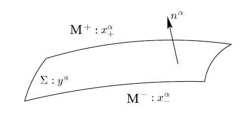
II.1 Kinematics of hypersurfaces

We have a $(3+1)$ manifold where there is a hypersurface $\Sigma$, with the condition $\Sigma\subset\mathcal{M}$ and $\Sigma$ can be either timelike, spacelike, or null. A specific hypersurface $\Sigma$ can be selected, when we restrict the coordinates $x^{\alpha}\in\mathcal{M}$ as

$$\Phi\left(x^{\alpha}\right)=0$$ (2)

and parametric equations as

$$x^{\alpha}=x^{\alpha}(y^{a}),\,\,\,x^{\alpha}\in\mathcal{M},\,\,\,y^{a}\in\Sigma\,\,\,\mbox{and}\,\,\,\Sigma\subset\mathcal{M},$$ (3)

where $y^{a}$ is intrinsic coordinates of $\Sigma$.

Additional, $\Sigma$ is characterized for a normal vector $n_{\alpha}$. This vector is unitary and is

$$n^{\alpha}n_{\alpha} =\epsilon$$

$$=-1,\,\,\,\mbox{If $\Sigma$ is spacelike.}$$

$$=1,\,\,\,\mbox{If $\Sigma$ is timelike.}$$ (4)

where

$$n_{\alpha}=\frac{\epsilon\partial_{\alpha}\Phi}{\sqrt{g^{\mu\nu}\partial_{\mu}\Phi\partial_{\nu}\Phi}}.$$ (5)

II.2 First fundamental form: induced metric

The induced metric is obtained when movements are limited on the hypersurface $\Sigma$. Such metric is

$$ds^{2}_{\Sigma}=h_{ab}dy^{a}dy^{b},\,\,\,h_{ab}=g_{\alpha\beta}e^{\alpha}_{a}e^{\beta}_{b},$$ (6)

where $h_{ab}$ is known as the induced metric or first fundamental form and tangent vectors to the integral curves in $\Sigma$ are

$$e^{\alpha}_{a}=\frac{\partial x^{\alpha}}{\partial y^{a}}.$$ (7)

II.3 Second fundamental form: extrinsic curvature

The intrinsic curvature of manifold $\mathcal{M}$ is determined for Riemann tensor, $R^{\alpha}_{\beta\gamma\delta}$

$$R^{\alpha}_{\beta\gamma\delta}=\frac{\partial\Gamma^{\alpha}_{\delta\beta}}{\partial x^{\gamma}}+\frac{\partial\Gamma^{\alpha}_{\gamma\beta}}{\partial x^{\delta}}+\Gamma^{\alpha}_{\gamma\sigma}\Gamma^{\sigma}_{\delta\beta}-\Gamma^{\alpha}_{\sigma\delta}\Gamma^{\sigma}_{\delta\beta}.$$ (8)

The extrinsic curvature or second fundamental form $K_{ab}$, defines how is curved $\Sigma$ hypersurface related to $\mathcal{M}$, it is embedded. So, $K_{ab}$ is related with normal derivative of metric tensor $g_{\alpha\beta}$

$$K_{ab}=\frac{1}{2}\left[\mathcal{L}_{n}g_{\mu\nu}\right]e^{\alpha}_{a}e^{\beta}_{b}=n_{\alpha;\beta}e^{\alpha}_{a}e^{\beta}_{b},$$ (9)

II.4 Formalism of Darmois-Israel

Being the hypersurface $\Sigma$, it divides spacetime in two regions $M^{+}$ and $M^{-}$, such that $g^{+}_{\alpha\beta}\in M^{+}$ and $g^{-}_{\alpha\beta}\in M^{-}$

Figure 1: Two regions of spacetime that joined in a common boundary. The Figure is take from PE .

II.5 The first condition of junction

The first condition of junction states: the induced metric in both sides of $\Sigma$ is the same one. We can take it, as the continuity of first fundamental form

$$\left[h_{ab}\right]=h_{ab}^{+}|_{\Sigma}-h_{ab}^{-}|_{\Sigma}=0.$$ (10)

II.6 Second condition of junction

This condition declares that the extrinsic curvature is the same in both sides of hypersurface $\Sigma$. This can be interpreted as the continuity of the second fundamental form

$$\left[K_{ab}\right]=K_{ab}^{+}|_{\Sigma}-K_{ab}^{-}|_{\Sigma}=0.$$ (11)

Both conditions are independent of global coordinates $x^{\alpha}$. Whether the second condition is broken, the spacetime is singular in $\Sigma$ and this is associated to presence of matter in the hypersurface as

$$S_{ab}=-\frac{\epsilon}{8\pi}\left(\left[K_{ab}\right]-\left[K\right]h_{ab}\right),\,\,\,K\equiv h^{ab}K_{ab}=n^{\alpha}_{;\alpha}.$$ (12)

Thus, the stress-energy tensor is correlated to the jump in extrinsic curvature from side of $\Sigma$ to other side. The stress-energy tensor on the hypersurface is defined as PE

$$T^{\alpha\beta}_{\Sigma}=\delta(l)S^{ab}e^{\alpha}_{\,a}e^{\beta}_{\,b}.$$ (13)

III The Shell Black in gravitational contraction

For a external observer in asymptotic far region, the sight correspond to a thin Shell which contracts close to the gravitational radius. Consequently, the spacetime around of this thin Shell, is symmetrically spherical and static

$$ds^{2}_{+}=-f(r)dt^{2}+\frac{1}{f(r)}dr^{2}+r^{2}d\theta^{2}+r^{2}\sin^{2}\theta d\phi^{2},$$ (14)

$$f(r)=1-\frac{2M}{r}$$

and inside of Shell, we have got Minkowski-like spacetime

$$ds^{2}_{-}=-dt^{2}+dr^{2}+r^{2}d\theta^{2}+r^{2}\sin^{2}\theta d\phi^{2}.$$ (15)

Figure 2: A thin Shell which is in a contraction close to the gravitational radius.

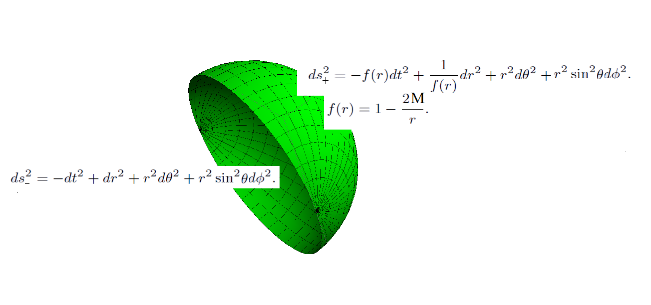
III.1 Internal solution $M^{-}$, $u^{\alpha}_{-}$, $n^{-}_{\alpha}$

The internal solution is flat, so we can choose the coordinates of $M^{-}$ as

$$t=\bar{T}(\tau),\,\,\,r=R(\tau),$$ (16)

thus, we have that (15) could be rewritten in terms of (16) as

$$ds^{2}_{-}=-\left[\dot{\bar{T}}^{2}(\tau)-\dot{R}^{2}(\tau)\right]d\tau^{2}+R^{2}(\tau)d\Omega^{2}.$$ (17)

On other hand, if we can choose the global coordinates as $x^{\alpha}_{-}=\left(\bar{T}(\tau),R(\tau),\theta,\phi,\right)$ and induced coordinates on $\Sigma$ as $y^{a}=\left(\tau,\theta,\phi\right)$, then, we find that 4-velocity is

$$u^{\alpha}_{-}=e^{\alpha}_{\tau}=\frac{\partial x^{\alpha}_{-}}{\partial\tau}=\left(\dot{\bar{T}}(\tau),\dot{R}(\tau),0,0\right).$$ (18)

Besides, we have the orthogonality conditions $n^{-}_{\alpha}u^{\alpha}_{-}=0$ and normalization conditions $n^{-}_{\alpha}n^{\alpha}_{-}=1$

$$n^{-}_{\alpha}=\left(-\dot{R}(\tau),\dot{\bar{T}}(\tau),0,0\right).$$ (19)

III.2 External solution $M^{+}$, $u^{\alpha}_{+}$, $n^{+}_{\alpha}$

The external solution is a Schwarzschild spacetime. Thus, we can choose the coordinates of $M^{+}$ as

$$t=T(\tau),\,\,\,r=R(\tau)\,\,\,\mbox{and}\,\,\,f(r)=F(R)=1-\frac{2M}{R}.$$ (20)

So, we have that (14) can be rewritten as

$$ds^{2}_{+}=-\left[FT(\tau)^{2}-\frac{\dot{R}^{2}(\tau)}{F}\right]d\tau^{2}+R^{2}(\tau)d\Omega^{2},$$ (21)

furthermore, the global coordinates are $x^{\alpha}_{+}=\left(T(\tau),R(\tau),\theta,\phi,\right)$ and induced coordinates are $y^{a}=\left(\tau,\theta,\phi\right)$. Then, the 4-velocity is

$$u^{\alpha}_{+}=e^{\alpha}_{\tau}=\frac{\partial x^{\alpha}_{+}}{\partial\tau}=\left(\dot{T}(\tau),\dot{R}(\tau),0,0\right).$$ (22)

As a result, we have the orthogonality conditions again $n^{+}_{\alpha}u^{\alpha}_{+}=0$ and normalization conditions $n^{+}_{\alpha}n^{\alpha}_{+}=1$

$$n^{+}_{\alpha}=\left(-\dot{R}(\tau),\dot{T}(\tau),0,0\right)$$ (23)

III.3 Shell motion equation

The Shell motion equation is obtained from (12)

$$\frac{dR}{d\tau}=\sqrt{\left[\frac{M}{\mu}+\frac{\mu}{2R}\right]^{2}-1},$$ (24)

Whether we define a new constant $a$ as the ratio between gravitational mass $M$ and rest mass $\mu$ of Shell, then we get

$$a=\frac{M}{\mu},\,\,\,\,\frac{dR}{d\tau}=\sqrt{\left[a+\frac{M}{2aR}\right]^{2}-1}.$$ (25)

Such parameter $a$ has got kinetic energy contribution and gravitational energy potential of particles of Shell. Israel defines $\mu$ is the nucleonic mass of particles of Shell, and also he affirms that the mass gravitational contains all energy forms: kinetic, gravitational and internal interaction among these particles (For this study is null) IW2 .

III.4 Conditions of Shell motion equation

It is possible to set up some conditions on kinematic of Shell from (25).That’s because for this equation the root cannot be negative, so, we have that

$$\left[a+\frac{\mu}{2aR}\right]^{2}-1\geq 0.$$

And, if we consider the upper limit $R=R_{\mbox{max}}$, we have IW2

$$R_{max}=\frac{M}{2a(1-a)}$$ (26)

At this point, is very import to take the conditions proposed by Israel about Shell motion equation. these are the following IW2

1. If the positive binding energy is $a=\cos\alpha<1$ and it is $E=(1-a)\mu<1$. Consequently Shell contracts from resting state with a finity radius $\dot{R}|_{R_{\mbox{max}}}=0$.

2. If $a=\cosh\alpha>1$, we obtain a negative binding energy. Thus, the Shell is impelled from infinity with initial velocity null $\dot{R}|_{R\longrightarrow\infty}=0$.

3. When $a=1$, the binding energy is zero, thus the internal pressure in the Shell also in zero. Thus, the Shell is a thin spherical layer of dust and this goes down from rest the resting state at $\dot{R}|_{R\longrightarrow\infty}=0$.

4. In particular case that $a\longrightarrow\infty$ then $\mu\longrightarrow a$ and therefore $M=a\mu$, the result is a Shell made of photons.

III.5 Israel’s solution to Shell motion equation

Being the Shell motion equation already established (25) there is an interest in studying the their case in the previous section. For this reason Israel presents the following set of solutions of the Shell motion equation IW2

$$r(\lambda)=M\left(\lambda^{2}-\frac{1}{4}\right),$$ (27)

$$t(\lambda)=M\left(\frac{2}{3}\lambda^{3}+\frac{5}{2}\lambda\right)+2M\ln\left|\frac{\lambda-3/2}{\lambda+3/2}\right|+C,$$ (28)

where $\lambda$ in (27) and (28) is a free parameter to the solution of (25), and $C$ is a constant that depends on the initial conditions in the kinematic of Shell. Is possible eliminate $\lambda$ in (27) and (28), so we obtain

$$t(r)=-M\left[\frac{2}{3}\left(\frac{r}{M}+\frac{1}{4}\right)^{3/2}+\frac{5}{2}\left(\frac{r}{M}+\frac{1}{4}\right)^{1/2}\right]+2M\ln\left|\frac{\sqrt{\frac{r}{M}+\frac{1}{4}}+3/2}{\sqrt{\frac{r}{M}+\frac{1}{4}}-3/2}\right|+C.$$ (29)

III.6 Arenas-Castro solution to Shell motion equation

Arenas-Castro JR presents an approximate solution to the Shell motion equation (25). Given the relation between the coordinate time $t$ and proper time $\tau$ LL as

$$d\tau=\sqrt{f(R)}dt,$$ (30)

where we assume the conditions of case 3, so we write the Shell motion equation as

$$\frac{1}{\sqrt{f(R)}}\frac{dR}{dt}=-\sqrt{\left[1+\frac{M}{2R}\right]^{2}-1},\,\,\,f(R)=1-\frac{2M}{R}.$$

$$\frac{dR}{d\tau}=-\sqrt{\left(1-\frac{2M}{R}\right)\left(\frac{M}{4R}+1\right)\frac{M}{R}}.$$ (31)

we define a function $g(R)$ as

$$g(R)=\sqrt{\left(1-\frac{2M}{R}\right)\left(\frac{M}{4R}+1\right)\frac{M}{R}}.$$ (32)

Then, for $g(R)$ defined in (32) another function $p(R)$ can be approximated to as

$$p(R)\approx K\left(\frac{M}{R}\right)\left(1-\frac{2M}{R}\right),\,\,\,K\approx 3.$$ (33)

In the Figure 3, we can note the behavior of $g(R)$ and $p(R)$. We choose $K$ under the following condition

$$\frac{dg(R)}{dr}|_{R=R_{max}}=0$$

Figure 3: The behavior of $g(R)$ and $p(R)$.

So, we can rewrite the Shell motion equation as

$$\frac{dR}{dt}=-K\left(\frac{M}{R}\right)\left(1-\frac{2M}{R}\right).$$ (34)

The integration of (34) is

$$\int^{r}_{r_{0}}\frac{dR}{\left(\frac{M}{R}\right)\left(1-\frac{2M}{R}\right)}=-3\int^{t_{s}}_{t_{0}}dt,$$

$$\frac{-6M(t_{s}-t_{0})-4M(r-r_{0})+(r^{2}-r_{0}^{2})}{8M^{2}}=\ln\left|\frac{r-2M}{r_{0}-2M}\right|,$$ (35)

where $r_{s}=2M$ is the Schwarzschild radius, $\Delta t=t_{s}-t_{0}$ and $\bar{\tau}=\frac{4}{3}M$. Then, the equation (35) reduces to

$$r-r_{s}=(r_{0}-r_{s})e^{-\frac{\Delta t}{\bar{\tau}}}e^{-\left[\frac{(r-r_{0})}{r_{s}}+\frac{(r^{2}-r_{0}^{2})}{2r_{s}^{2}}\right]}.$$ (36)

It is possible define a new function $\bar{F}$ in the equation (36)

$$\bar{F}=e^{-\left[\frac{(r-r_{0})}{r_{s}}+\frac{(r^{2}-r_{0}^{2})}{2r_{s}^{2}}\right]},$$ (37)

the function $\bar{F}$ is expanded in a Taylor series as $e^{x}=\sum_{n=0}^{\infty}\frac{x^{n}}{n!}$ and it has an approximation to Zero order. Thus, $\bar{F}\approx 1$ and (36) reduces to

$$r(t)=r_{s}+\underbrace{(r_{0}-r_{s})}_{\Delta r}e^{-\frac{\Delta t}{\bar{\tau}}}=r_{s}+\Delta re^{-\frac{\Delta t}{\bar{\tau}}}.$$ (38)

We rewrite the equation (38) as

$$t(r)=\bar{\tau}\ln\left|\frac{r_{0}-r_{s}}{r-r_{s}}\right|,\,\,\,\bar{\tau}=\frac{4}{3}M$$ (39)

III.7 Akhmedov-Godazgar-Popov solution to the Shell motion equation

Recently, Akhmedov-Godazgar-Popov AE presented a new Shell motion equation. In this paper, this equation is interpreted as a new condition of the Shell evolution, additional to Israel’s conditions. As a result, the movement of Shell has these stages

• The Shell is remained fixed at some $r(t)=r_{0}$ by an additional force (see Figure 4).

• This phase is a highly tuned stage of collapse if one wishes to respect spherical symmetry.

• The final phase describes stage where the Shell collapses.

Figure 4: The movement of Shell that is seen by an external observer in a asymptotic far region. The Figure is taken from AE .

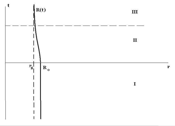
Akhmedov-Godazgar-Popov obtained the Shell motion equation from the first condition of junction, (10). Thus, they found that

$$\dot{\bar{T}}^{2}-\dot{R}^{2}=F\dot{T}^{2}-\frac{\dot{R}^{2}}{F}.$$ (40)

Nevertheless, the normal vectors $n_{\alpha}^{+}$ and $n_{\alpha}^{-}$ to $\Sigma$ are defined in (19) and (23). This vectors obey the orthonormalization condition (4). So, we can take equation (40) write and find

$$\dot{\bar{T}}^{2}-\dot{R}^{2}=F\dot{T}^{2}-\frac{\dot{R}^{2}}{F}=1.$$ (41)

In the light of this, Akhmedov-Godazgar-Popov discovered a new Shell motion equation which was

$$\left(\frac{dt_{-}}{d\tau}\right)^{2}-\left(\frac{dR}{d\tau}\right)^{2}=\left(1-\frac{2M}{R}\right)\left(\frac{dt_{+}}{d\tau}\right)^{2}-\frac{1}{\left(1-\frac{2M}{R}\right)}\left(\frac{dR}{d\tau}\right)^{2}=1,$$

$$\left(1-\frac{2M}{R}\right)\left(\frac{dt_{+}}{d\tau}\right)^{2}-\frac{1}{\left(1-\frac{2M}{R}\right)}\left(\frac{dR}{d\tau}\right)^{2}=1.$$ (42)

To determine solution for the new Shell motion equation, they proposed the following set of conditions on Shell motion

1. The Shell velocity measured by comovil observer when $\frac{dR}{d\tau}\neq 0$ is not null, non zero, around the gravitational radius.

2. Also, the relation between the coordinate times $t_{+}$ and $t_{-}$ is

   $$dt_{-}=\sqrt{f(r_{s})}dt_{+},\,\,\,f(r_{s})=1-\frac{2M}{r_{s}},\,\,\,\mbox{when}\,\,\,t_{+}\leq 0,$$ (43)

   then, this quantity diverges when

   $$\lim_{t_{+}\to\infty}\frac{dt_{+}}{d\tau}=\infty.$$ (44)

3. Additionally $\left|R-r_{s}\right|\ll r_{s}$.

On the condition that right handside in comparison to the left handside is neglect in the new Shell motion equation, (42),then it’s found that

$$\left(1-\frac{2M}{R}\right)\left(\frac{dt_{+}}{d\tau}\right)^{2}-\frac{1}{\left(1-\frac{2M}{R}\right)}\left(\frac{dR}{d\tau}\right)^{2}\approx 0.$$ (45)

The integration of (45) is

$$-\int^{t_{s}}_{t_{0}}dt_{+}=\int^{r}_{r_{0}}\frac{1}{1-\frac{2M}{R}}dR$$

$$-(t_{s}-t_{0})=r-r_{0}+2M\ln\left|\frac{r-2M}{r_{0}-2M}\right|$$ (46)

after short simplification, they found

$$r-2M=(r_{0}-2M)e^{-(r-r_{0})/2M}e^{-\Delta t/2M},\,\,\,\Delta t=t_{s}-t_{0}.$$ (47)

Once again, we can specify a new function $\bar{F}=e^{-(r-r_{0})/2M}\approx 1$. Then, the solution to the Shell motion is

$$r(t)=r_{s}+\Delta re^{-\Delta t/2M},\,\,\,r_{s}=2M.$$ (48)

We rewrite the equation (48) as

$$t(r)=r_{s}\ln\left|\frac{r_{0}-r_{s}}{r-r_{s}}\right|.$$ (49)

III.8 Comparison between the solutions to the Shell motion equation

In this section, the comparison among the several solutions that we review previously, is presented. The solutions already taken into account have been considered as the solutions for the Shell motion equation, according to an external observer’s sight.

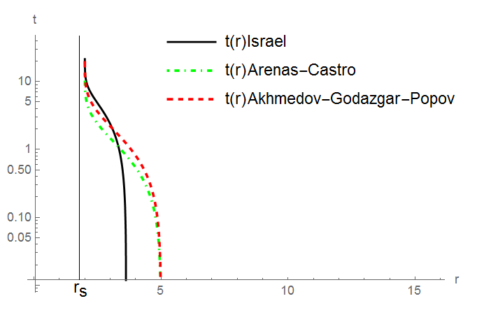
In the Figure 5, we can note this solutions comparison. The $t$ and $x$ axes are in cartesian coordinates. When the Shell is close to Schwarzschild radius, all solutions converge to same behavior.

Figure 5: Comparison of several solutions of the Shell motion equation close to Schwarzschild radius. The axes are in cartesian coordinates.

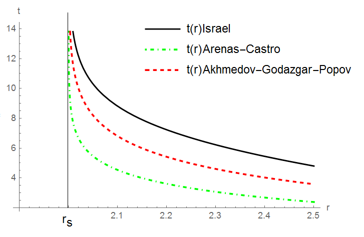
Once more, in the Figure 6 the behavior of the solutions studied is shown, where the $t$ axis is in logarithmic scale AE . In addition, we can see the same behavior for the solutions analyzed, when the Shell is close to horizon.

Figure 6: Comparison of the several solutions of the Shell motion equation close to Schwarzschild radius. The $t$ axis is in logarithmic scale AE .

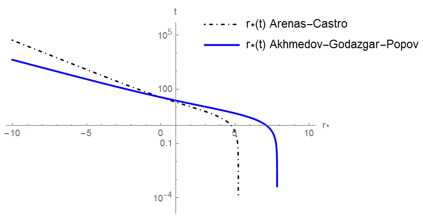
Moreover, the Arenas-Castro (38) and Akhmedov-Godazgar-Popov (48) solutions can rewritten in turtle coordinates WR , $r^{*}=r+2M\ln\left|\frac{r}{2M}-1\right|$. So we find that (38) reduces to

$$r^{*}_{\mbox{Arenas-Castro}}(t)=r^{*}_{0}-\frac{3}{2}t+\left(r_{s}-r_{0}\right)\left[1-e^{-t/\bar{\tau}}\right],\,\,\,r^{*}_{0}=r_{0}+r_{s}\ln\left|\frac{r_{0}}{r_{s}}-1\right|\,\,\,\mbox{y}\,\,\,\bar{\tau}=\frac{4}{3}M$$ (50)

and also (48)

$$r^{*}_{\mbox{Akhmedov-Godazgar-Popov}}(t)=r^{*}_{0}-t+\left(r_{s}-r_{0}\right)\left[1-e^{-t/\bar{2M}}\right],\,\,\,r^{*}_{0}=r_{0}+r_{s}\ln\left|\frac{r_{0}}{r_{s}}-1\right|.$$ (51)

In the Figure 7, we observe the Arenas-Castro and Akhmedov-Godazgar-Popov solutions in turtle coordinates. This graph allows us to see that $\Sigma$ is timelike hypersurface , which turns to be null hypersurface, when $r^{*}_{i}(t)\longrightarrow r_{s}$ AE

Figure 7: The Arenas-Castro and Akhmedov-Godazgar-Popov solutions in turtle coordinates.

III.9 Behavior of the Shell near to horizon

We take the Arenas-Castro solution for Shell movement in (38)

$$r(t)=r_{s}+\Delta re^{-\frac{\Delta t}{\bar{\tau}}},\,\,\,\bar{\tau}=\frac{4}{3}M,$$ (52)

where $t$ is the coordinate time for an external observer.
The Shell movement can be parametrized as

$$r(t)=nr_{s},\,\,\,r_{s}=2M.$$ (53)

As a result, the Shell goes from a distance leaving the resting state $n$ times the gravitational radius, and it stops when is near by the horizon

$$r(t_{0})=r_{0}=2Mnr_{s},\,\,\,r(t_{1})=r_{s},\,\,\,t_{1}\gg t_{0}.$$ (54)

In the same way, the coordinate time can be expressed as $n$ times the Planck time as

$$t=nt_{p}.$$ (55)

Also, we have that $\Delta r$ is rewritten as (see next section about this equation)

$$\epsilon=2\Delta r=2nl_{p}.$$ (56)

Replacing the (54)-(56) equations in (52) it is obtained

$$n=\frac{1}{2M}\left[2M+ne^{-\frac{3n}{4M}}\right].$$ (57)

The equation (57) is solved when the Shell mass is know (we try several parametric form to the (55) and (56) equations, having the same result.)

$M_{\odot}$	n
$10^{0}$	$1.24469$
$10^{1}$	$1.04846$
$10^{2}$	$1.00499$
$10^{3}$	$1.00050$
$10^{4}$	$1.00005$
$10^{5}$	$1.00000$
$10^{6}$	$1.00000$

Table 1: Numerical solution of the equation (57) for different solar mass $M_{\odot}$.

In the chart 1, it is observed that the value $n=1$ is independent of solar mass of Shell. As a consequence we fin it from (56) that

$$\epsilon=2l_{p},$$ (58)

as the minimum value that $\epsilon$ can taken near by the horizon. This is import, because for an external observer is able to see that the Shell movement is stops near to the Schwarzschild radius and never goes beyond from this point.
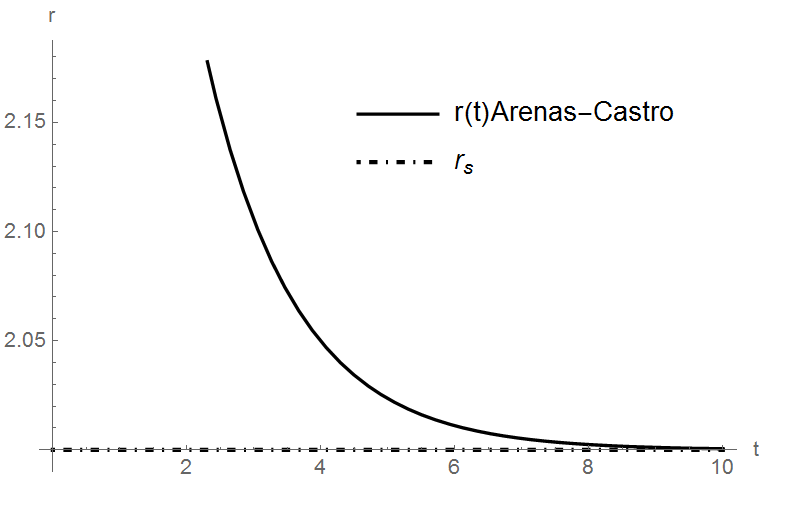
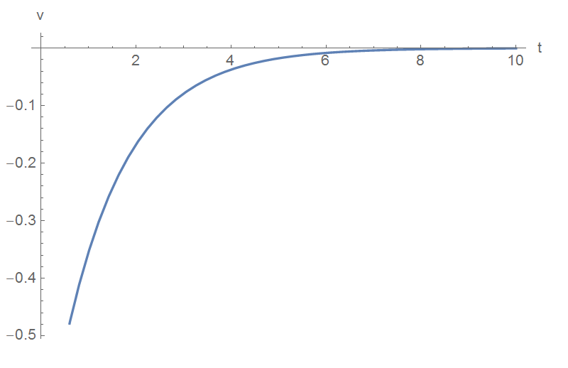
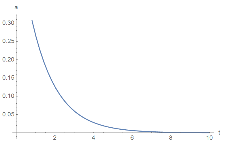
In the Figures 9 to 11, the Shell’s kinematic is presented according to the Arenas-Castro solution. So, for an external observer, the Shell movement is stopped, its 3-velocity and 3-acceleration are null close to the gravitational radius. In such conditions, any effect can be attributed to the presence of the horizon, due to the fact that the inner region $r<2M$ far beyond is completely unknown for any external observer. Also, the minimal distance between the horizon and the Shell is $\epsilon=2l_{p}$ for finite time equal to universe age. Just when

$$\lim_{t\to\infty}r(t)=r_{s}.$$ (59)

III.10 Thermodynamics properties of the Dirac’s field near to gravitational radius.

The spacetime around the Shell in gravitational contraction is

$$ds^{2}=-f(r)dt^{2}+\frac{1}{f(r)}dr^{2}+r^{2}d\theta^{2}+r^{2}\sin^{2}d\phi^{2},\,\,\,f(r)=1-\frac{2M}{r}.$$ (60)

The Shell movement, here, is described by the Arenas-Castro solution JR

$$r(t)=r_{s}+\Delta re^{-t/\bar{\tau}},\,\,\,\,\Delta r=r_{0}-r_{s},\,\,\,\,r_{s}=\frac{2GM}{c^{2}},\,\,\,\,\bar{\tau}=\frac{4GM}{3c^{3}}.$$ (61)

Furthermore, for great values of the coordinate time we have that

$$\lim_{t\longrightarrow t_{p}}r(t)=r_{s}.$$

Therefore, we calculate the differential from equation (61) and the result is

$$\frac{dr}{dt}=-\frac{\Delta re^{-t/\bar{\tau}}}{\bar{\tau}}.$$ (62)

Where the $(-)$ in the equation (62), shows that the ratio is decreasing related to the coordinate time.

Figure 8: The Shell is in gravitational contraction from infinity to near the horizon.

The entropy of the Dirac field close to horizon under high energies approximation MS ; RW3 corresponds to a description of standard statistical physics. Also, particles with rest-mass $m$, energy $E$, 3-momentum $p$ and 3-velocity, that are measures for an external observer. So, the density energy $\rho$, pressure $P$ and entropy density $s(r)$ are

$$\rho=-\int^{\infty}_{0}\frac{E}{e^{E/T(r)}+1}\frac{4\pi^{2}}{h^{3}},$$ (63)

$$p=\frac{1}{3}\int^{\infty}_{0}\frac{pv}{e^{E/T(r)}+1}\frac{4\pi^{2}}{h^{3}}dp,$$ (64)

$$S=\int_{Vol}s\,dV,\,\,\,s=\beta(\rho+P)=\frac{4NT^{3}}{\pi^{2}},$$ (65)

where $N$ is quantum fields number and their helicities, the local temperature $T(r)$ which is given by Tolman’s law TR

$$T(r)=\frac{T_{\infty}}{\sqrt{f(r)}}.$$ (66)

Thus, 3-volume differential element $dV$, is determinated by

$$dV=\frac{4\pi}{\sqrt{f(r)}}r^{2}dr=\frac{4\pi}{\sqrt{f(r)}}\left(r_{s}+\Delta re^{-t/\bar{\tau}}\right)^{2}\frac{\Delta re^{-t/\bar{\tau}}}{\bar{\tau}}dt.$$ (67)

With an approximation to the first order, we have than $\Delta r\gg\Delta r^{2},\Delta r^{3}$. Therefore, the 3-volume differential element reduces to

$$dV\approx\frac{4\pi}{\sqrt{f(r)}}\left(\frac{r_{s}^{2}\Delta re^{-t/\bar{\tau}}}{\bar{\tau}}\right)dt.$$ (68)

So the equation (65) is rewritten follows

$$S=\frac{4N}{\pi^{2}}T_{\infty}^{3}\frac{4\pi r_{s}^{2}}{\bar{\tau}}\Delta r\int\frac{e^{t/\bar{\tau}}}{f^{2}(r)}dt,$$ (69)

where, the horizon area is $A_{\mathcal{H}}=4\pi r_{s}^{2}$ and $f(r)=f(r(t))$. Near to the Schwarzschild radius, we have that this can be reexpressed as

$$f(r(t))\approx 2\kappa_{0}(r(t)-r_{s})=2\kappa_{0}\Delta re^{-t/\bar{\tau}},$$ (70)

where the surface gravity on the horizon is MS

$$\kappa_{0}=-\frac{1}{2}\frac{df(r)}{dr}|_{r=r_{s}}=\frac{1}{4M}.$$ (71)

After short simplification in the equation (69), we find

$$S=\frac{4N}{\pi^{2}}\left(\frac{T_{\infty}^{3}}{\kappa_{0}^{2}}\right)\frac{A_{\mathcal{H}}}{4}\frac{1}{\Delta r}\left[\frac{1}{\bar{\tau}}\int^{t_{u}}_{0}e^{t/\bar{\tau}}dt\right],$$ (72)

where the integral in the equation (72) corresponds to a dimensionless constant depending on the coordinate time as

$$C_{1}=\frac{1}{\bar{\tau}}\int^{t_{u}}_{0}e^{t/\bar{\tau}}dt.$$ (73)

Thus, the equation (72) according to (73), is reduces to

$$S=\frac{4N}{\pi^{2}}\left(\frac{T_{\infty}^{3}}{\kappa_{0}^{2}}\right)\frac{A_{\mathcal{H}}}{4}\frac{1}{\Delta r}C_{1}.$$ (74)

On the other hand, the proper altitude above the horizon $\alpha$ is LL

$$\alpha=\int^{r_{1}}_{r_{0}}\frac{dr}{\sqrt{f(r)}}=\frac{1}{\bar{\tau}}\int^{t_{u}}_{0}\frac{\Delta re^{-t/\bar{\tau}}}{\sqrt{2\kappa_{0}\Delta re^{-t/\bar{\tau}}}}dt=\sqrt{\frac{\Delta r}{2\kappa_{0}}}\left[\frac{1}{\bar{\tau}}\int^{t_{u}}_{0}e^{-t/\bar{\tau}}dt\right].$$ (75)

The expossed previously is rewritten in terms of a additional constant as

$$\alpha=\sqrt{\frac{\Delta r}{2\kappa_{0}}}C_{2},$$ (76)

$$C_{2}=\frac{1}{\bar{\tau}}\int^{t_{u}}_{0}e^{-t/\bar{\tau}}dt.$$ (77)

hence, the Dirac field entropy, (74), near by to horizon is reduced to

$$S_{\mbox{Shell}}=\left[\frac{N}{90\pi\alpha^{2}}\left(\frac{T_{\infty}}{\kappa_{0}/2\pi}\right)^{3}\frac{A}{4}\right]\frac{C_{1}C^{2}_{2}}{4}=\frac{S_{\mbox{BWM}}}{4}C_{1}C^{2}_{2},$$ (78)

where $S_{\mbox{BMW}}$ is the entropy for quantum fields, and it works according to Mukohyama-Israel MS . Also, whether $S_{\mbox{BWM}}=S_{\mbox{Shell}}$ and $\Delta r_{\mbox{BWM}}=\Delta r_{\mbox{Shell}}$, we can have the values for the constants, so

$$C_{1}=1,\,\,\,C_{2}=\pm 2.$$ (79)

And the Dirac field entropy is

$$\Delta r_{\mbox{Shell}}=\frac{4\Delta r_{\mbox{BWM}}}{C^{2}_{2}},\,\,\,\Delta r_{\mbox{BWM}}=\frac{1}{2}\kappa_{0}\alpha^{2}.$$ (80)

$$S_{\mbox{Shell}}=\frac{N}{90\pi\alpha^{2}}\left(\frac{T\infty}{\kappa_{0}/2\pi}\right)^{3}\frac{A}{4},\,\,\,\Delta r_{\mbox{Shell}}=\frac{\kappa_{0}\alpha^{2}}{2}.$$ (81)

An external observer can measure that the temperature of the Dirac field is equal to Hawking temperature, $T_{\infty}=T_{H}=\frac{\kappa_{0}}{2\pi}$ , so the the Dirac field entropy is

$$S_{\mbox{Shell}}=S_{BH}=\frac{1}{4}\frac{A}{l_{p}^{2}},$$ (82)

and the proper altitude above the horizon, $\alpha$ MS is

$$\alpha=l_{P}\sqrt{\frac{C_{1}C^{2}_{2}N}{360\pi}}=l_{P}\sqrt{\frac{N}{90\pi}}.$$ (83)

III.11 About the values of the constants $C_{1}$ and $C_{2}$

The equation (73) is rewritten as

$$\frac{dC_{1}}{dt}=\frac{1}{\bar{\tau}}e^{t/\bar{\tau}},$$

$$\frac{dC_{1}}{dr}\frac{dr}{dt}=\frac{1}{\bar{\tau}}e^{t/\bar{\tau}},$$

where $dr/dt$ is given by (61) and the times coordinate by (39). Then, $C_{1}$ is reduced

$$C_{1}=-\Delta r\int_{r_{0}}^{r_{s}+\epsilon}\frac{1}{(r-r_{s})^{2}}dr=\frac{r_{0}-r_{s}-\epsilon}{\epsilon}=\frac{\Delta r}{\epsilon}-1.$$ (84)

The physical analysis of (84) is complex, since their values can be in a different order of magnitude

$$r_{0}\sim 10^{23}m,\,\,\,r_{s}\sim 10^{3}m\,\,\,y\,\,\,\epsilon\sim 10^{-35}m,$$

All the above, considering a black hole of one solar mass, $m_{\odot}\sim 10^{30}kg$. So, under these conditions, a different approach should be considered, as the values of $r$ multiples of Schwarzschild radius, $r_{s}$. Therefore, we can write

$$r_{0}=r_{s}*10^{m},\,\,\,\epsilon=r_{s}*10^{-n},$$

Thus, we have that the initial radius $r_{0}$ and the cutoff $\epsilon$ are multiples from gravitational radius $r_{s}$. Thus $m$ and $n$ are not necessarily integer

$$-\infty\leq m,n\leq\infty.$$

In the special case that $m=n=0$, we find

$$C_{1}=\frac{10^{m}-1-10^{-n}}{10^{-n}}=10^{m+n}-10^{-n}-1,$$ (85)

$$C_{1}=10^{2m}-10^{-m}-1=1.$$ (86)

This coincides with Mukohyama- Israel method MS , owing to the minimum value that takes $C_{1}$ close to horizon, that is

$$C_{1}(r_{s}+\epsilon)=1,$$ (87)

also the ratio between $C_{1}$ and the coordinate time $t$, is an increasing function

$$\frac{dC_{1}}{dt}=\frac{1}{\bar{\tau}}e^{t/\bar{\tau}}.$$ (88)

For the value of $C_{2}$, from the equation (77), can be rewritten as

$$\frac{dC_{2}}{dt}=\frac{1}{\bar{\tau}}e^{-t/\bar{\tau}},$$ (89)

where (89) has a boundary condition $C_{2}(r_{s}+\epsilon)=2$, so we have

$$\frac{dC_{2}}{dr}\left(\frac{dr}{dt}\right)=\frac{1}{\bar{\tau}}e^{-t/\bar{\tau}},$$ (90)

also, (90) is reduced to

$$\frac{dC_{2}}{dr}=-\frac{1}{\Delta r}.$$ (91)

And integrating the equation (91), we have

$$C_{2} =-\frac{1}{\Delta r}\int^{r_{s}+\epsilon}_{r_{0}}dr$$

$$=\frac{1}{\Delta r}\left[\Delta r-\epsilon\right]=1-\frac{\epsilon}{\Delta r}=1-\frac{\epsilon}{r_{0}-r_{s}}$$

$$\propto\frac{1}{r_{0}}.$$ (92)

This implies that, $C_{2}$ is an decreasing function, where under the boundary condition $C_{2}(r_{s}+\epsilon)=2$. So that, $\epsilon$ is reduces to

$$\epsilon=-\Delta r.$$ (93)

Nevertheless, whether we consider the ratio $\frac{C_{1}}{C_{2}}$ as

$$\frac{C_{1}}{C_{2}}=\frac{\Delta r}{\epsilon},$$ (94)

$$\epsilon=\frac{C_{2}}{C_{1}}\Delta r.$$ (95)

Then is possible define a new constant $n|_{r_{s}+\epsilon}$ as

$$n|_{r_{s}+\epsilon}=\left(\frac{C_{2}}{C_{1}}\right)_{r_{s}+\epsilon}=2,$$ (96)

so, the minimum value that $\epsilon$ that is got to the horizon is

$$\epsilon|_{r_{s}+\epsilon}=n\Delta r=2\Delta r$$ (97)

Along this analysis, we have to take into account that the constants $C_{i}$ and $\epsilon$ arose from the Shell’s kinematic.

Once, we have the Dirac’s field entropy near to horizon, $S_{\mbox{Shell}}$, we can calculate other thermodynamics properties of fermionic field. So, we write from equation (78)

$$S_{\mbox{Shell}}=\frac{N\pi^{2}}{180\alpha^{2}}\left(\frac{T^{3}_{\infty}}{\kappa^{3}_{0}}\right)A\,C_{1}C^{2}_{2}.$$ (98)

• The Helmholtz free energy, $F$ is written as

  $$S_{\mbox{Shell}}=-\left(\frac{\partial F}{\partial T_{\infty}}\right)_{V},$$

  $$F=-\frac{N\pi^{2}}{720\alpha^{2}}\left(\frac{T^{4}_{\infty}}{\kappa^{3}_{0}}\right)AC_{1}C^{2}_{2}.$$ (99)

• The internal energy, $E$

  $$dE=dF+T_{\infty}dS,$$

  $$E=\frac{N\pi^{2}}{240\alpha^{2}}\left(\frac{T^{4}_{\infty}}{\kappa^{3}_{0}}\right)AC_{1}C^{2}_{2}.$$ (100)

• The specific heat capacity at a volume constant ($C_{V}$) and the specific heat capacity at pressure constant ($C_{P}$) are

  $$C_{V}=\left(\frac{\partial E}{\partial T_{\infty}}\right)_{V},\,\,\,C_{P}=T_{\infty}\left(\frac{\partial S}{\partial T_{\infty}}\right)_{P},$$ (101)

  also ZM

  $$\lim_{T\to T_{H}}C_{V}=C_{P},\,\,\,T_{H}=\frac{1}{8\pi M_{\odot}}\approx 10^{-8}K.$$ (102)

  therefore, we find

  $$C_{V}=C_{P}=\frac{N\pi^{2}}{60\alpha^{2}}\left(\frac{T^{3}_{\infty}}{\kappa^{3}_{0}}\right)AC_{1}C^{2}_{2}.$$ (103)

• And the internal pressure is calculated ($P$) as

  $$P=-\left(\frac{\partial F}{\partial V}\right)_{T_{\infty}}=-\frac{1}{\alpha}\left(\frac{\partial F}{\partial A}\right)_{T_{\infty}}$$

  As a result we obtain

  $$P=\frac{N\pi^{2}}{720\alpha^{3}}\left(\frac{T^{3}_{\infty}}{\kappa^{3}_{0}}\right)C_{1}C^{2}_{2}.$$ (104)

In this point, is very relevant to mention that if the Shell’s entropy is equal to BWM entropy, we have $S_{\mbox{Shell}}=S_{\mbox{BWM}}$. And if $C_{1}=1$, $C_{2}=2$, the species number $N=1$ for the quantum fields, also the proper altitude above the horizon $\alpha$ given by (83). Then, the thermodynamics properties are reduce to

$$S_{\mbox{Shell}}=\frac{\pi^{2}}{45\alpha^{2}}\left(\frac{T^{3}_{\infty}}{\kappa^{3}_{0}}\right)A.$$ (105)

$$F=-\frac{\pi^{2}}{180\alpha^{2}}\left(\frac{T^{4}_{\infty}}{\kappa^{3}_{0}}\right)A.$$ (106)

$$E=\frac{\pi^{2}}{60\alpha^{2}}\left(\frac{T^{4}_{\infty}}{\kappa^{3}}_{0}\right)A.$$ (107)

$$C_{V}=C_{P}=\frac{\pi^{2}}{15\alpha^{2}}\left(\frac{T^{3}_{\infty}}{\kappa^{3}_{0}}\right)A.$$ (108)

$$P=\frac{\pi^{2}}{180\alpha^{3}}\left(\frac{T^{3}_{\infty}}{\kappa^{3}_{0}}\right).$$ (109)

These properties coincides with RW1 ; RW2 , for the spacetime $3+1$ and the spacetime $D+1$ with a scalar hot quantum field.

IV The species problem

Now, we consider the species problem for the entanglement entropy, for fermionic field RW3 and bosonic field MS ; FD ; RW1 ; RW2 ; JR2 near by the horizon.

The fermionic field entropy RW3 , (105), is

$$S_{\mbox{F}}=\frac{\pi^{2}}{45\alpha^{2}}\left(\frac{T^{3}_{\infty}}{\kappa^{3}_{0}}\right)A$$ (110)

and the internal energy of fermionic field (107) is

$$E_{\mbox{F}}=\frac{\pi^{2}}{60\alpha^{2}}\left(\frac{T^{4}_{\infty}}{\kappa_{0}^{3}}\right)A.$$ (111)

The unification of (110) and (111) with $\beta=\frac{1}{T_{\infty}}$ CY is

$$S_{\mbox{F}}=\frac{4}{3}\beta E_{\mbox{F}}.$$ (112)

In the same way, for bosonic field, we have that the entropy MS ; RW1 ; RW2 ; JR2 is

$$S_{\mbox{B}}=\frac{1}{90\pi\alpha^{2}}\left(\frac{T^{3}_{\infty}}{\left(\kappa_{0}/2\pi\right)^{3}}\right)A$$ (113)

And the free energy is

$$S=-\left(\frac{\partial F}{\partial T_{\infty}}\right)_{V},$$ (114)

$$F_{\mbox{B}}=-\frac{\pi^{2}}{180\alpha^{2}}\left(\frac{T^{4}_{\infty}}{\kappa_{0}^{3}}\right)A.$$ (115)

So, the internal energy $E$ is

$$dE=dF-T_{\infty}dS$$ (116)

$$E_{\mbox{B}}=\frac{\pi^{2}}{60\alpha^{2}}\left(\frac{T^{4}_{\infty}}{\kappa_{0}^{3}}\right)A.$$ (117)

This shows that for the quantum fields studied, we find that

$$E=E_{\mbox{B}}=E_{\mbox{F}}=\frac{\pi^{2}}{60\alpha^{2}}\left(\frac{T^{4}_{\infty}}{\kappa_{0}^{3}}\right)A.$$ (118)

For this reason, the entropy of the bosonic field $S_{\mbox{B}}$ is written as

$$S_{\mbox{B}}=\frac{4}{3}\beta E_{\mbox{B}}.$$ (119)

Whether the quantum fields are in thermal equilibrium, among themselves and the horizon, the product is

$$T_{\mbox{B}}=T_{\mbox{F}}=T_{H}.$$

Also, the total entropy is the sum of the partial entropies of every field, so we get

$$S =S_{\mbox{B}}+S_{\mbox{F}}$$

$$=\frac{4}{3}\beta E_{\mbox{B}}+\frac{4}{3}\beta E_{\mbox{F}}$$

$$=\frac{4}{3}\beta\left[E_{\mbox{B}}+E_{\mbox{F}}\right]$$

$$=\frac{4}{3}\beta E,\,\,\,\,E=E_{\mbox{B}}+E_{\mbox{F}}.$$ (120)

Moreover, from the equation (118), the equation (120) is rewritten as

$$S=\frac{8}{3}\beta\frac{\pi^{2}}{60\alpha^{2}}\left(\frac{T_{\infty}^{4}}{\kappa_{0}^{3}}\right)A,$$ (121)

where $\beta=1/\frac{1}{T_{\infty}}$. For the proper altitude above the horizon, $\alpha$, which was defined previously, (83)

$$\alpha=l_{P}\sqrt{\frac{N}{90\pi}}.$$ (122)

where $N=2$, for quantum fields, if these fields are in thermal equilibrium with the horizon at a temperature Hawking, $T_{H}=\frac{\kappa_{0}}{2\pi}$. This results in the Bekenstein-Hawking entropy, $S_{BH}$

$$S=\frac{1}{4}\frac{A}{l_{p}^{2}}.$$ (123)

This result is very interesting, due to the Bekenstein-Hawking entropy for black holes is independent of the quantum fields near to horizon, their nature, their spins and the internal interaction of quantum fields researched.

The Bekenstein-Hawking entropy arose from thermal atmosphere around the horizon, which is seen by an external observer in a far asymptotic region.

V Summary and Discussion

Along this paper, we review the Shell equations and their kinematic behavior near by the Schwarzschild radius. Also, we chose a solution for the Shell motion equation, so it was possible to determine the minimal value of cutoff close to the horizon for the entanglement entropy for the Dirac’s field

$$\epsilon|_{r_{s}+\epsilon}=n\Delta r=2\Delta r.$$ (124)

So that, we found the entanglement entropy for the Dirac’s field near by the gravitational radius as

$$S_{\mbox{Shell}}=S_{\mbox{F}}=\frac{\pi^{2}}{45\alpha^{2}}\left(\frac{T^{3}_{\infty}}{\kappa^{3}_{0}}\right)A,$$ (125)

where $\alpha$ is the proper altitude above the horizon, according to (75).

With the condition that $T_{\infty}=T_{H}=\frac{\kappa_{0}}{2\pi}$, $S_{\mbox{Shell}}$ coincides with $S_{BH}=\frac{1}{4}\frac{A}{l_{p}}$.

About the species problem, we showed for a case of two fields that the entropy is independent of nature and the number of fields near to the horizon:

$$S_{\mbox{Ent}}=S_{\mbox{B}}+S_{\mbox{F}}=\frac{4}{3}\beta E=\frac{1}{4}\frac{A}{l_{p}^{2}},$$ (126)

where $\beta=\frac{1}{T_{\infty}}$, $T_{\infty}=T_{H}$ and $E=E_{\mbox{B}}+E_{\mbox{F}}$. The Bekenstein-Hawking entropy, $S_{BH}$ arise from thermal atmosphere around to the horizon.

We consider that this result is completely generalizable for any number of fields.

Appendix A The Shell motion equation

A.1 Extrinsic curvature seen from $M^{+}$

Once, the normal vector $n^{\alpha}$ is known, is possible calculate the extrinsic curvature from (9)

$$K_{\alpha\beta}=n_{\alpha;\beta},$$ (127)

this calculated on external solution, $M^{+}$, then we have

$$K^{+}_{\theta\theta}=\dot{T}RF,\,\,\,K^{+\theta}_{\theta}=g^{\theta\theta}K^{+}_{\theta\theta}=\frac{\beta_{+}}{F},\,\,\,\beta_{+}=\dot{T}F$$ (128)

$$K^{+}_{\phi\phi}=\dot{T}RF\sin^{2}\theta,\,\,\,K^{+\phi}_{\phi}=g^{\phi\phi}K^{+}_{\phi\phi}=\frac{\beta_{+}}{R}$$ (129)

and finally

$$K^{+}_{\tau\tau}=-F^{\prime}\dot{T},\,\,\,K^{+\tau}_{\tau}=g^{\tau\tau}K^{+}_{\tau\tau}=\frac{\dot{\beta}_{+}}{F},\,\,\,\dot{\beta}_{+}=F^{\prime}\dot{R}\dot{T}.$$ (130)

A.2 Extrinsic curvature seen from $M^{-}$

As it was developed in the last section, the extrinsic curvature components for external, $M^{-}$, solution are

$$K^{-}_{\theta\theta}=\dot{T}R,\,\,\,K^{-\theta}_{\theta}=g^{\theta\theta}K^{-}_{\theta\theta}=\frac{\beta_{-}}{R},\,\,\,\beta_{-}=\sqrt{1-\dot{R}^{2}}$$ (131)

$$K^{-}_{\phi\phi}=\dot{\dot{T}}R\sin^{2}\theta,\,\,\,K^{-\phi}_{\phi}=g^{\phi\phi}K^{-}_{\phi\phi}=\frac{\beta_{-}}{R}$$ (132)

$$K^{-}_{\tau\tau}=0,\,\,\,K^{-\tau}_{\tau}=g^{\tau\tau}K^{-}_{\tau\tau}=0$$ (133)

A.3 The Shell motion equation

The Shell motion equation is obtained from the equation (12)

$$S^{a}\,_{b}=-\frac{\epsilon}{8\pi}\left(\left[K^{a}\,_{b}\right]-\left[K\right]h^{a}\,_{b}\right),\,\,\,K\equiv h^{ab}K_{ab}=n^{\alpha}_{;\alpha}.$$ (134)

Besides, it is obtained by using the orthonormal condition of the induced metric, $h^{a}\,_{a}=1$. So from this equation (134), we have that

$$S^{\tau}\,_{\tau} =-\frac{\epsilon}{8\pi}\left[K^{+\tau}\,_{\tau}-K^{-\tau}\,_{\tau}-\left(K^{+}-K^{-}\right)h^{\tau}\,_{\tau}\right]$$

$$=-\frac{\epsilon}{8\pi}\left[K^{+\tau}\,_{\tau}-K^{-\tau}\,_{\tau}-K^{+\tau}\,_{\tau}+K^{-\tau}\,_{\tau}-K^{+\theta}\,_{\theta}+K^{-\theta}\,_{\theta}-K^{+\phi}\,_{\phi}+K^{-\phi}\,_{\phi}\right]$$

$$=-\frac{\epsilon}{8\pi}(-2)\left[K^{+\theta}\,_{\theta}-K^{-\phi}\,_{\phi}\right].$$ (135)

With the values of $K^{+\theta}\,_{\theta}$ and $K^{-\phi}\,_{\phi}$ defined in (128) and (132), the equation (135) is rewritten as

$$S^{\tau}\,_{\tau}=-\frac{\epsilon}{8\pi}(-2)\left[\frac{\beta_{+}}{R}-\frac{\beta_{-}}{R}\right].$$ (136)

The surface tensor $S^{ab}=\sigma u^{a}u^{b}$ is write as $S^{a}\,_{b}=\sigma u^{a}u_{b}$, also with the normalization condition for 4-velocity $u^{a}u_{a}=-1$, we find

$$S^{a}\,_{a}=\sigma u^{a}u_{a}=-\sigma,\,\,\,S^{\tau}\,_{\tau}=-\sigma.$$ (137)

Replacing (137) into (136), we obtain

$$-\sigma=\frac{1}{4\pi}\left[\frac{\beta_{+}}{R}-\frac{\beta_{-}}{R}\right]$$ (138)

in the same way, for the $S^{\theta}\,_{\theta}$ component

$$S^{\theta}\,_{\theta}=-\frac{\epsilon}{8\pi}\left[K^{+\theta}\,_{\theta}-K^{-\theta}\,_{\theta}-\left(K^{+}-K^{-}\right)h^{\theta}\,_{\theta}\right]$$ (139)

After replaced all the values of the extrinsic curvature, $K^{+a}\,_{a}$ and $K^{-a}\,_{a}$, it is found that

$$-\frac{\epsilon}{8\pi}\left[-\frac{\dot{\beta}_{+}}{\dot{R}}-\frac{\beta_{+}}{R}+\frac{\beta_{-}}{R}\right]=0.$$ (140)

This is rewritten as

$$\frac{\dot{\beta}_{+}}{\dot{R}}=\frac{\beta_{-}}{R}-\frac{\beta_{+}}{R}.$$ (141)

Where, we have that $\beta_{+}=\dot{T}F$, $\dot{\beta}_{+}=F^{\prime}\dot{R}\dot{T}$ and $\beta_{-}^{2}=1+\dot{R}^{2}$. Furthermore, we impose following condition

$$K^{-\tau}\,_{\tau}=0\longrightarrow\dot{\beta}_{-}=0.$$ (142)

So

$$\dot{\beta}_{+}=\frac{d}{d\tau}\left[\beta_{+}-\beta_{-}\right].$$ (143)

So that, the equation (140) is simplificated to

$$\frac{d}{d\tau}\left[\beta_{+}-\beta_{-}\right]=\frac{1}{R}\frac{dR}{d\tau}\left[\beta_{-}-\beta_{+}\right]$$ (144)

The integration of (144) is

$$\int\frac{d\left(\beta_{+}-\beta_{-}\right)}{\beta_{-}-\beta_{+}}=\int\frac{dR}{R}\longrightarrow C=R\left(\beta_{-}-\beta_{+}\right).$$ (145)

Well, if we are agree with (138)

$$4\pi\sigma R^{2}=R\left(\beta_{-}-\beta_{+}\right)=C.$$ (146)

In this point, we can define the rest mass of the Shell, $\mu=C$

$$\mu=R\left(\beta_{-}-\beta_{+}\right)\longrightarrow\beta_{+}=\beta_{-}-\frac{\mu}{R}.$$ (147)

Getting the square root out of this and taking into account that $\beta_{-}^{2}=\dot{R}^{2}+1$, $\beta^{2}_{+}=\dot{R}^{2}+F$ and $F=1-\frac{2M}{R}$, where $M$ is the gravitational mass and $M\neq\mu$. $M$ contains kinetic energy and potential gravitational for the Shell in gravitational contraction.

Therefore, we have

$$\beta_{+}^{2}=\beta_{-}^{2}-\frac{2\beta_{-}\mu}{R}+\frac{\mu^{2}}{R^{2}}=1+\dot{R}^{2}-\frac{2\mu}{R}\sqrt{1+\dot{R}^{2}}+\frac{\mu^{2}}{R^{2}}$$ (148)

$$\frac{2M}{R}=\frac{2\mu}{R}\sqrt{1+\dot{R}^{2}}-\frac{\mu^{2}}{R^{2}},$$ (149)

the last equation is rewritten as

$$\frac{dR}{d\tau}=\sqrt{\left[\frac{M}{\mu}+\frac{\mu}{2R}\right]^{2}-1},$$ (150)

we define the ratio between the gravitational mass $M$ and rest mass $\mu$ of the Shell as

$$a=\frac{M}{\mu},\,\,\,\,\frac{dR}{d\tau}=\sqrt{\left[a+\frac{M}{2aR}\right]^{2}-1}.$$ (151)

Appendix B The Shell kinematic

In this appendix, we were able to draw the 3-position, 3-velocity and 3-acceleration of Shell, that is seen by an external observer in a flat and far asymptotic region for the Arenas-Castro solution

Figure 9: The Shell 3-position to the equation (52).

Figure 10: The Shell 3-velocity.

Figure 11: The Shell 3-acceleration.

Appendix C Acknowledgments

I want to thank Javier Cano and Walter Pulido for their valuable observations during the development of my research work.

This work was supported by the Departamento de Administrativo de Ciencia, Tecnología e Innovación, Colciencias.

References

- (1) Bekenstein J. D. Phys. Rev. D 7, 2333 (1973).
- (2) Hawking, S. W. Comm. Math. Phys. 43, 199 (1975).
- (3) Gibbons, G. W. and Hawking, S. W. Phys. Rev. D 15, 2752 (1977).
- (4) ’t Hooft, G. Nucl. Phys. B256, 727 (1985).
- (5) J. R. Arenas S. Tesis de Doctorado: Termodinámica de entanglement del efecto Unruh. Departamento de Física. Universidad Nacional de Colombia. Director: Juan Manuel Tejeiro Sarmiento (2005).
- (6) D. V. Fursaev. Phys. Part. Nucl. 36 (2005):81.
- (7) Mukohyama S. and Israel W. Phys. Rev. D58,104005 (1998).
- (8) Pretorius, F. and Vollick, D. and Israel, W. Phys. Rev. D57 (1998),6311-6316.
- (9) Poisson, E. A Relativist’s Toolkit: The Mathematics of Black-Hole Mechanics. Cambridge University Press (2004).
- (10) Israel, W. Nuovo Cimento B Serie, jul 44 (1966)1-14.
- (11) Carroll, S.M. Spacetime and Geometry: An Introduction to General Relativity. Addison Wesley (2004).
- (12) Israel, W. Phys. Rev. 153, 5 (1967), 1388-1393.
- (13) J. Frauendiener and C. Klein. J. Math. Phys. 36 (1995) 3632.
- (14) Kijowski, J. and Magli, G. and Malafarina, D. General Relativity and Gravitation vol:38,11 (2006) 1697-1713.
- (15) Canonico, R. Doctoral Thesis: Exact solutions in general relativity and alternative theories of gravity: mathematical and physical properties. Universita degli studi di Salerno (2010).
- (16) Bengtsson, Ingemar and Jakobsson, Emma and Senovilla, José M. M. Phys. Rev. D88 (2013).
- (17) Grøn, Ø. and Hervik, S. Einstein’s General Theory of Relativity: With Modern Applications in Cosmology. Springer New York (2007).
- (18) J. R, Arenas S. and F. Castro. arXiv: 1606.06786 [gr-qc].
- (19) Landau, L.D. and Lifshitz, E.M. Curso de física teórica. Reverté (1973).
- (20) Akhmedov, E. T. , Godazgar, H. and Popov, F. K. Phys. Rev. D93, 024029 (2016).
- (21) Wald, R.M. General Relativity. University of Chicago Press (2010).
- (22) Tolman, R.C. Relativity, thermodynamics and cosmology. The Clarendon Press (1934).
- (23) W. A. Rojas C. and J. R. Arenas S. arXiv: 1110.4058 [gr-qc].
- (24) W. A. Rojas C. and J. R. Arenas S. arXiv:1607.00042 [gr-qc].
- (25) Zemansky, M.W. and Dittman, R.H. International series in pure and applied mathematics / McGraw-Hill (1997).
- (26) Jacobson T. arXiv: 9404039 [gr-qc].
- (27) Chen, Yu-Zhu and Li, Wen-Du and Dai, Wu-Sheng. arXiv: 1609.00787 [gr-qc].
- (28) J. R. Arenas S. and J. M. Tejeiro S. Nuovo Cim. B125 (2010) 1223-1248.
- (29) W. A. Rojas C. Tesis de Doctorado: Mecánica Estadística de Termodinámica de Black Shells. Departamento de Física. Universidad Nacional de Colombia. Director: J. R. Arenas S. (2018).