Pruning based Distance Sketches with Provable Guarantees on Random Graphs

Abstract.

Measuring the distances between vertices on graphs is one of the most fundamental components in network analysis. Since finding shortest paths requires traversing the graph, it is challenging to obtain distance information on large graphs very quickly. In this work, we present a preprocessing algorithm that is able to create landmark based distance sketches efficiently, with strong theoretical guarantees. When evaluated on a diverse set of social and information networks, our algorithm significantly improves over existing approaches by reducing the number of landmarks stored, preprocessing time, or stretch of the estimated distances.

On Erdos-Renyi graphs and random power law graphs with degree distribution exponent $2<\beta<3$, our algorithm outputs an exact distance data structure with space between $\Theta(n^{5/4})$ and $\Theta(n^{3/2})$ depending on the value of $\beta$, where $n$ is the number of vertices. We complement the algorithm with tight lower bounds for Erdos-Renyi graphs and the case when $\beta$ is close to two.

1. Introduction

Computing shortest path distances on large graphs is a fundamental problem in computer science and has been the subject of much study (Thorup and Zwick, 2005; Goldberg and Harrelson, 2005; Sommer, 2014). In many applications, it is important to compute the shortest path distance between two given nodes, i.e. to answer shortest path queries, in real time. Graph distances measure the closeness or similarity of vertices and are often used as one of the most basic metric in network analysis (He et al., 2007; Potamias et al., 2009; Vieira et al., 2007; Yahia et al., 2008). In this paper, we will focus on efficient and practical implementations of shortest path queries in classes of graphs that are relevant to web search, social networks, and collaboration networks etc. For such graphs, one commonly used technique is that of landmark-based labelings: every node is assigned a set of landmarks, and the distance between two nodes in computed only via their common landmarks. If the set of landmarks can be easily computed, and is small, then we obtain both efficient pre-processing and small query time.

Landmark based labelings (and their more general counterpart, Distance Labelings), have been studied extensively (Sommer, 2014; Bast et al., 2016). In particular, a sequence of results culminating in the work of Thorup and Zwick (Thorup and Zwick, 2005) showed that labeling schemes can provide a multiplicative 3-approximation to the shortest path distance between any two nodes, while having an overhead of ${O}({\sqrt{n}})$ storage per node on average in the graph (we use the standard notation that a graph has $n$ nodes and $m$ edges). In the worst case, there is no distance labeling scheme that always uses sub-quadratic amount of space and provides exact shortest paths. Even for graphs with maximum degree $3$, it is known that any distance labeling scheme requires $\Omega(n^{3/2})$ total space (Gavoille et al., 2001). In sharp contrast to these theoretical results, there is ample empirical evidence that very efficient distance labeling schemes exist in real world graphs that can achieve much better approximations. For example, Akiba et al. (Akiba et al., 2013) and Delling et al. (Delling et al., 2014a) show that current algorithms can find landmark based labelings that use only a few hundred landmarks per vertex to obtain exact distance, in a wide collection of social, Web, and computer networks with millions of vertices. In this paper, we make substantial progress towards closing the gap between theoretical and observed performance. We show that natural landmark based labeling schemes can give exact shortest path distances with a small number of landmarks for a popular model of (unweighted and undirected) web and social graphs, namely the heavy-tailed random graph model. We also formally show how further reduction in the number of landmarks can be obtained if we are willing to tolerate an additive error of one or two hops, in contrast to the multiplicative 3-approximation for general graphs. Finally, we present practical versions of our algorithms that result in substantial performance improvements on many real-world graphs.

In addition to being simple to implement, landmark based shortest path algorithms also offer a qualitative benefit, in that they can directly be used as the basis of a social search algorithm. In social search (Bahmani and Goel, 2012), we assume there is a collection of keywords associated with every node, and we need to answer queries of the following form: given node $v$ and keyword $w$, find the node that is closest to $v$ among all nodes that have the keyword $w$ associated with them. This requires an index size that is $O(L)$ times the size of the total social search corpus and a query time of $O(L)$, where $L$ is the number of landmarks per node in the underlying landmark based algorithm; the approximation guarantee for the social search problem is the same as that of the landmark based algorithm. Thus, our results lead to both provable and practical improvements to the social search problem.

Existing models for social and information networks build on random graphs with some specified degree distribution (Durrett, 2007; Chung and Lu, 2006; Van Der Hofstad, 2009), and there is considerable evidence that real-world graphs have power-law degree distributions (Clauset et al., 2009; Eikmeier and Gleich, 2017). We will use the Chung-Lu model (Chung and Lu, 2002), which assumes that the degree sequence of our graph is given, and then draws a “uniform” sample from graphs that have the same or very similar degree sequences. In particular, we will study the following question: Given a random graph from the Chung-Lu model with a power law degree distribution of exponent $\beta$, how much storage does a landmark-based scheme require overall, in order to answer distance queries with no distortion?

In the rest of the paper, we use the term “random power law graph” to refer to a graph that is sampled from the Chung-Lu model, where the weight (equivalently, the expected degree) of each vertex is independently drawn from a power law distribution with exponent $\beta$. We are interested in the regime when $\beta>2$ — this covers most of the empirical power law degree distributions that people have observed on social and information networks (Clauset et al., 2009). Admittedly, real-world graphs have additional structure in addition to having power-law degree distributions (Leskovec et al., 2008), and hence, we have also validated the effectiveness of our algorithm on real graphs.

1.1. Our Results

Our first result corresponds to the “easy regime”, where the degree distribution has finite variance ($\beta>3$). We show that a simple procedure for generating landmarks guarantees exact shortest paths, while only requiring each node to store $\tilde{O}(\sqrt{n})$ landmarks. The same conclusion also applies to Erdős-Renyi graphs $G(n,\frac{c}{n})$ when $c>1$, or when $c=2\log n$.

We then study the case where $2<\beta<3$. This is the most emblematic regime for power-law graphs, since the degree distribution has infinite variance but finite expectation. We present an algorithm that generates at most $\tilde{O}(n^{\scriptscriptstyle(\beta-2)/(\beta-1)})$ landmarks per node when $\beta\geq 2.5$; and $\tilde{O}(n^{\scriptscriptstyle(3-\beta)/(4-\beta)})$ landmarks per node when $2<\beta<2.5$. We obtain additional improvements if we allow an additive error of 1 or 2. See Figure 1 for an illustration of our results.

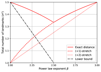
Figure 1. An illustration of the results for labeling schemes: The $x$-axis is the exponent of the power law degree distribution and each value on the $y$-axis corresponds to a storage of $\tilde{\textsc{O}}(n^{y})$. The lower bound curve is for exact distances.

While the dependence on $\beta$ is complex, it is worth noting that in the entire range that we study ($\beta>2$), the number of landmarks per node is at most $\tilde{O}({\sqrt{n}})$ for exact shortest paths. This is in stark contrast to known impossibility results for general graphs, where no distance labeling with a multiplicative stretch less than 3 can use sub-linear space per node (Gavoille et al., 2001). The query time of our algorithms is proportional to the number of landmarks per node, so we also get speed improvements.

Our algorithm is based on the pruned labeling algorithm of Akiba et al. (Akiba et al., 2013), but differs in important ways. The pruned labeling algorithm initially posits that every node is a landmark for every other node, and then uses the BFS tree from each node to iteratively prune away unnecessary landmarks. In our approach, we apply a similar BFS with pruning procedure on a small subset of $H$ (i.e. high degree vertices), but switch to lightweight local ball growing procedures up to radius $l$ for all other vertices. As we show, the original pruned labeling algorithm requires storing $\tilde{\Omega}(n^{2})$ landmarks on sparse Erdös-Rényi graphs. By growing local balls of size $\sqrt{n}$, our algorithm recovers exact distances with at most $\tilde{O}(n^{3/2})$ landmarks instead, for Erdös-Rényi graphs and random power law graphs with $\beta>3$. Hence, our algorithm combines exploiting the existence of high-degree “central landmarks” with finding landmarks that are “locally important”. Furthermore for $2<\beta<3$, by setting up the number of global landmarks $H$ and the radius $l$ suitably, we provably recover the upper bounds described in Figure 1. While the algorithmic idea is quite simple, the analysis is intricate.

We complement our algorithmic results with tight lower bounds for the regime when $\beta>3$: the total length of any distance labeling schemes that answer distance queries exactly in this regime is almost surely $\tilde{\Omega}(n^{1.5})$. We also show that when $2<\beta<2.5$, any distance labeling scheme will generate labels of total size $\tilde{\Omega}(n^{3.5-\beta})$ almost surely. In particular, our algorithm achieves the optimal bound when $\beta$ is close 2.

The parameter choice suggested by our theoretical analysis can be quite expensive to implement (as can earlier landmark based algorithms). We apply a simple but principled parameter tuning procedure to our algorithm that substantially improves the preprocessing time and generates a smaller set of landmarks at essentially no loss of accuracy. We conduct experiments on several real world graphs, both directed and undirected. First, compared to the pruned labeling algorithm, we find that our algorithm reduces the number of landmarks stored by 1.5-2.5x; the preprocessing time is reduced significantly as well. Next, we compare our algorithm to the distance oracle of Thorup and Zwick (Thorup and Zwick, 2005), which is believed to be theoretically optimal for worst-case graphs, as well as the distance sketch of Das Sarma et al (Das Sarma et al., 2010) which has been found to be both efficient and useful in prior work (Bahmani and Goel, 2012). For each graph, our algorithm substantially outperforms these two benchmarks. Details are in Section 5. It is important to note that the three algorithms we compare to also work much better on these real-world graphs than their theoretical guarantee, and we spend considerable effort tuning their parameters as well. Hence, the performance improvement given by our algorithm is particularly noteworthy.

It is worth mentioning that our technical tools only rely on bounding the growth rate of the breadth-first search. Hence we expect that our results can be extended to the related configuration model (Durrett, 2007) as well. One limitation of our work is that the analysis does not apply directly to preferential attachment graphs, which correspond to another family of well known power law graphs. But we believe that similar results can be obtained there by adapting our analysis to that setting as well. This is left for future work.

Organizations: The rest of the paper is organized as follows. Section 2 introduces the basics of random graphs, reviews the pruned labeling algorithm and related work. Section 3 introduces our approach. Section 4 analyzes our algorithm on random power law graphs. Then we present experiments in Section 5. We show the lower bounds in Section 6. We conclude in Section 7. The Appendix contains missing proofs from the main body.

2. Preliminaries and Related Work

2.1. Notations

Let $G=(V,E)$ be a directed graph with $n=\left\lvert V\right\rvert$ vertices and $m=\left\lvert E\right\rvert$ edges. For a vertex $x\in V$, denote by $d_{out}(x)$ the outdegree of $x$ and $d_{in}(x)$ the indegree of $x$. Let $\mathcal{N}_{out}(x)$ denote the set of its out neighbors. Let $\mathrm{dist}_{G}(x,y)$ denote the distance of $x$ and $y$ in $G$, or $\mathrm{dist}(x,y)$ for simplicity. When $G$ is undirected, then the outdegrees and indegrees are equal. Hence we simply denote by $d_{x}$ the degree of every vertex $x\in V$. For an integer $l$ and $x\in V$, denote by $\Gamma_{l}(x)=\{y:\mathrm{dist}(x,y)=l\}$ the set of vertices at distance $l$ from $x$. Denote by $N_{l}(x)$ the set of vertices at distance at most $l$ from $x$.

We use notation $a\lesssim b$ to indicate that there exists an absolute constant $C>0$ such that $a\leq Cb$. The notations $\tilde{O}(\cdot)$ and $\tilde{\Omega}(\cdot)$ hide poly-logarithmic factors.

2.2. Landmark based Labelings

In a landmark based labeling (Delling et al., 2014b), each vertex $x$ is assigned a set of forward landmarks $L_{F}(x)$ and backward landmarks $L_{B}(x)$. Each landmark set is a hash table, whose keys are vertices and values are distances. For example, if $y\in L_{F}(x)$, then the value associated with $y$ would be $\mathrm{dist}(x,y)$, which is the “forward” distance from $x$ to $y$. Given the landmark sets $L_{F}(\cdot)$ and $L_{B}(\cdot)$, we estimate the distances as follows:

(1) $$\min_{z\in L_{F}(x)\cap L_{B}(y)}\mathrm{dist}(x,z)+\mathrm{dist}(z,y),\forall x,y\in V.$$

If no common vertex is found between $L_{F}(x)$ and $L_{B}(y)$, then $y$ is not reachable from $x$. In the worst case, computing set intersection takes $\Omega(\min(\left\lvert L_{F}(x)\right\rvert,\left\lvert L_{B}(y)\right\rvert))$ time.

Denote the output of equation (1) by $\hat{d}$. Clearly, we have $\hat{d}\geq\mathrm{dist}(x,y)$ when $y$ is reachable from $x$. The additive stretch of $\hat{d}$ is given by $\hat{d}-\mathrm{dist}(x,y)$, and the multiplicative stretch is given by $\hat{d}/\mathrm{dist}(x,y)$. When there are no errors for any pairs of vertices, such landmark sets are called 2-hop covers (Cohen, 1997).

There is a more general family of data structures known as labeling schemes (Gavoille et al., 2001), which associates a vector $\mathcal{L}:V\rightarrow\{0,1\}^{*}$ for every vertex. When answering a query for a pair of vertices $x,y\in V$, only the two labels $\mathcal{L}(x)$ and $\mathcal{L}(y)$ are required without accessing the graph. The total length of $\mathcal{L}$ is given by $\sum_{x\in V}|\mathcal{L}(x)|$. It is clear from equation (1) that landmark sketches fall in the query model of labeling schemes.

2.3. The Pruned Labeling Algorithm

We review the pruned labeling algorithm (Akiba et al., 2013) for readers who are not familiar. The algorithm starts with an ordering of the vertices, $\{x_{1},x_{2},\dots,x_{n}\}$. First for $x_{1}$, a breadth first search (BFS) is performed over the entire graph. During the BFS, $x_{1}$ is added to the landmark set of every vertex. Next for $x_{2}$, in addition to running BFS, a pruning step is performed before adding $x_{2}$ as a landmark. For example, suppose that a path of length $l$ is found from $x_{2}$ to $y$. If $x_{1}$ lies on the shortest path fom $x_{2}$ to $y$, then by checking their landmark sets, we can find the common landmark $x_{1}$ to certify that $\mathrm{dist}(x_{2},y)=\mathrm{dist}(x_{2},x_{1})+\mathrm{dist}(x_{1},y)\leq l$. In this case, $x_{2}$ is not added to $y$’s landmark set, and the neighbors of $y$ are pruned away. The above procedure is repeated on $x_{3}$, $x_{4}$, etc.

For completeness, we describe the pseudocode in Algorithm 1. Note that the backward BFS procedure can be derived similarly. It has been shown that the pruned labeling algorithm is guaranteed to return exact distances (Akiba et al., 2013).

Algorithm 1 PrunedLabeling (Akiba et al. (Akiba et al., 2013))

1:A directed graph $G=(V,E)$; An ordering of $V$, $\{x_{1},x_{2},\dots,x_{n}\}$.

2:Let $\mathcal{O}=\varnothing$, and $L_{F}(x)=L_{B}(x)=\varnothing$, for all $x\in V$

3:for $i=1,\dots,n$ do

4:    forwardBfs($x_{i}$)

5:    backwardBfs($x_{i}$)

6:    $\mathcal{O}=\mathcal{O}\cup\{x_{i}\}$

7:end for

8:

9:procedure forwardBfs($x_{i}$)

10:    Let $Q$ be a priority queue and $S$ be a hash set

11:    Set the priority of $x_{i}$ to be zero

12:    while $Q\neq\varnothing$ do

13:         Let $l$ be the minimum priority of $Q$

14:         Let $u$ be the corresponding vertex

15:         $S=S\cup\{u\}$

16:         Let $\tilde{d}=\min_{y\in L_{F}(x_{i})\cap L_{B}(u)}\mathrm{dist}(x_{i},y)+\mathrm{dist}(y,u)$

17:         if $l<\tilde{d}$ then (otherwise $u$’s neighbors are pruned)

18:             $L_{B}(u)=L_{B}(u)\cup\{x_{i}\rightarrow l\}$

19:             for $y\in\mathcal{N}_{out}(u)$ such that $y\notin\mathcal{O}$ do

20:                 Let $q$ be the priority of $y$

21:                 if $y\notin S$ and $l+1<q$ then

22:                     Decrease $y$’s priority to $l+1$

23:                 end if

24:             end for

25:         end if

26:    end while

27:end procedure

2.4. Random Graphs

We review the basics of Erdös-Rényi random graphs. Let $G=G(n,p)$ be an undirected graph where every edge appears with probability $p$. It is well known that when $p\geq 2(\log n)/n$, $G$ has only one connected component with high probability. Moreover, the neighborhood growth rate (i.e. $\left\lvert\Gamma_{i+1}(x)\right\rvert/\left\lvert\Gamma_{i}(x)\right\rvert$) is highly concentrated around its expectation, which is $np$. Formally, the following facts are well-known.

Fact 1 (Bollobás (Bollobás, 1998)).

Let $G=(V,E)$ be an undirected graph where every edge is sampled with probability $p=2(\log n)/n$. Let $D=\lceil\frac{\log n}{\log(np)}\rceil$. Then the following are true with high probability:

• The diameter of $G$ is at most $D+1$;

• For any $x,y\in V$ and $l\leq D$, $\Pr(\mathrm{dist}(x,y)\leq l)\leq\frac{(np)^{l+1}}{n(np-1)}$;

• For any $x\in V$ and $l<D$, we have $\frac{1}{2}\leq\frac{\left\lvert\Gamma_{l}(x)\right\rvert}{(np)^{l}}\leq 2$.

The Chung-Lu model: Let $p_{x}>0$ denote a weight value for every vertex $x\in V$. Given the weight vector $\mathbf{p}$, the Chung-Lu model generalizes Erdös-Rényi graphs such that each edge is chosen independently with probability

$$\Pr[x\sim y]=\min\left\{\frac{p_{x}\cdot p_{y}}{\mathrm{vol}(V)},1\right\},\forall x,y\in V$$

where $\mathrm{vol}(V)=\sum_{x\in V}p_{x}$ denote the volume of $V$.

Random power law graphs: Let $f:[x_{\min},\infty)\rightarrow\mathbb{R}$ denote the probability density function of a power law distribution with exponent $\beta>1$, i.e. $f(x)=Zx^{-\beta}$, where $Z=(\beta-1)\cdot x_{\min}^{\beta-1}$ (Clauset et al., 2009). The expectation of $f(\cdot)$ exists when $\beta>2$. The second moment is finite when $\beta>3$. When $\beta<3$, the expectation is finite, but the empirical second moment grows polynomially in the number of samples with high probability. If $\beta<2$, then even the expectation becomes unbounded as $n$ grows.

In a random power law graph, the weight of each vertex is drawn independently from the power law distribution. Given the weight vector $\mathbf{p}$, a random graph is sampled according to the Chung-Lu model. If the average degree $\nu>1$, then it is known that almost surely the graph has a unique giant component (Chung and Lu, 2006).

2.5. Related Work

Landmark based labelings: There is a rich history of study on how to preprocess a graph to answer shortest path queries (Abraham and Gavoille, 2011; Alstrup et al., 2015; Althöfer et al., 1993; Cohen, 1997; Thorup and Zwick, 2005; Borassi et al., 2017a). It is beyond our scope to give a comprehensive review of the literature and we refer the reader to survey (Sommer, 2014) for references.

In general, it is NP-hard to compute the optimal landmark based labeling (or 2-hop cover). Based on an LP relaxation, a $\log n$ factor approximation can be obtained via a greedy algorithm (Cohen et al., 2003). See also the references (Angelidakis et al., 2017; Babenko et al., 2015; Delling et al., 2014b; Goldberg et al., 2013; Borassi et al., 2017b) for a line of followup work. The current state of the art is achieved based on the pruned labeling algorithm (Akiba et al., 2013; Delling et al., 2014a). Apart from the basic version that we have already presented, bit-parallel optimizations have been used to speed up proprocessing (Akiba et al., 2013). Variants which can be executed when the graph does not fit in memory have also been studied (Jiang et al., 2014). It is conceivable that such techniques can be added on top of the algorithms that we study as well. For the purpose of this work, we will focus on the basic version of the pruned labeling algorithm. Compared to classical approaches such as distance oracles, the novelty of the pruned labeling algorithm is using the idea of pruning to reduce redundancy in the BFS tree.

Network models: Earlier work on random graphs focus on modeling the small world phenomenon (Chung and Lu, 2006), and show that the average distance grows logarithmically in the number of vertices. Recent work have enriched random graph models with more realistic features, e.g. community structures (Kolda et al., 2014), shrinking diameters in temporal graphs (Leskovec et al., 2010).

Other existing mathematical models on special families of graphs related to distance queries include road networks (Abraham et al., 2010), planar graphs and graphs with doubling dimension. However none of them can capture the expansion properties that have been observed on sub-networks of real-world social networks (Leskovec et al., 2008).

Previous work of Chen et al. (Chen et al., 2009) presented a 3-approximate labeling scheme requiring storage $\tilde{O}(n^{(\beta-2)/(2\beta-3)})$ per vertex, on random power law graphs with $2<\beta<3$. Our (+2)-stretch result improves upon this scheme in the amount of storage needed per vertex for $2<\beta<2.5$, with a much better stretch guarantee. Another related line of work considers compact routing schemes on random graphs. Enachescu et al. (Enachescu et al., 2008) presented a 2-approximate compact routing scheme using space $O(n^{\scriptscriptstyle 1.75})$ on Erdös-Rényi random graphs, and Gavoille et al. (Gavoille et al., 2015) obtained a 5-approximate compact routing scheme on random power law graphs.

3. Our Approach

In order to motivate the idea behind our approach, we begin with an analysis of the pruned labeling algorithm on Erdös-Rényi random graphs. While the structures of real world graphs are far from Erdös-Rényi graphs, the intuition obtained from the analysis will be useful. Below we describe a simple proposition which states that for sparse Erdös-Rényi graphs, the pruned labeling algorithm outputs $\tilde{\Omega}(n^{2})$ landmarks.

Proposition 1.

Let $G=(V,E)$ be an undirected Erdös-Rényi graph where every edge appears with probability $p=2(\log n)/n$. For any ordering of the vertices $V=\{x_{1},x_{2},\dots,x_{n}\}$, with high probability over the randomness of $G$, the total number of landmarks produced by Algorithm 1 is at least $\tilde{\Omega}(n^{2})$.

Proof sketch.

We first introduce a few notations. Let $r=np$ denote the growth rate of $G$. Let $\varepsilon=1/\log n$. Consider a vertex $x_{i}$ where $1\leq i\leq\varepsilon n$. Denote by $X_{-i}=\{x_{1},\ldots,x_{i-1}\}$. Consider any $u\in V$, if none of the shortest paths from $x_{i}$ to $u$ intersect with $X_{-i}$, then $(x_{i},u)$ is called a bad pair. Note that $x_{i}$ must be added to $u$’s landmark set by Algorithm 1, because during the BFS from $x_{i}$, all estimates through $X_{-i}$ will be strictly larger than $\mathrm{dist}(x_{i},u)$. Hence, to lower bound the total landmark sizes, it suffices to count the number of bad pairs. In the following, we show that in expectation for every $x_{i}$ where $1\leq i\leq\varepsilon n$, there are at least $n/(\log n)^{3}$ vertices $u$ such that $(x_{i},u)$ are bad. It follows that Algorithm 1 requires at least $\varepsilon n^{2}/(\log n)^{3}\geq\tilde{\Omega}(n^{2})$ in expectation.

Let $D=\lfloor\log_{r}n-2\rfloor$. Consider $\Gamma_{D}(x_{i})$, the set of vertices at distance equal to $D$ from $x_{i}$. We count the number of bad vertices in $\Gamma_{D}(x_{i})$ at follows. For each $1\leq k\leq D$, consider the intersection $\Gamma_{k}(x_{i})\cap X_{-i}$ and their subtree down to $\Gamma_{D}(x_{i})$.

Starting from any $y\in\Gamma_{k}(x_{i})\cap X_{-i}$, the subtree of $y$ would result in good vertices in $\Gamma_{D}(x_{i})$, whose distance from $x_{i}$ can be correctly estimated (c.f. line 15-16 in Algorithm 1). In expectation, the size of the intersection is $r^{k}\varepsilon$, because the probability that any two vertex has distance $k$ on $G$ is equal to $r^{k}/n$, and there are at most $\varepsilon n$ vertices in $X_{-i}$. Next, each $y$ results in $r^{D-k}$ vertices in its $(D-k)$-th level neighborhood. Combined together, the total number of good vertices which are covered by $\Gamma_{k}(x_{i})\cap X_{-i}$ is at most $r^{k}\varepsilon\times r^{D-k}=\varepsilon r^{D}$. By summing over all $k\leq D$, we obtain that the total number of good vertices in $\Gamma_{D}(x_{i})$ is at most $D\varepsilon r^{D}$.

On the other hand, the size of $\Gamma_{D}(x_{i})$ is $r^{D}$. Hence the total number of bad vertices is at least $(1-D\varepsilon)r^{D}\geq n/\log^{3}n$. To show that the the proposition holds with high probability, it suffices to apply concentration results on neighborhood growth in the arguments above. We omit the details.

∎

The interesting point from the above analysis is that $\Theta(n)$ landmarks are added throughout the first $\varepsilon n$ vertices. The reason is that there are no high degree vertices in Erdös-Rényi graphs, hence the landmarks we have added in the beginning do not cover the shortest paths for many vertex pairs later.Secondly, a large number of distant vertices are added in the landmark sets, which do not lie on the shortest paths of many pairs of vertices.

Motivated by the observation, we introduce our approach as follows. We start with an ordering of the vertices. For the top $H$ vertices in the ordering, we perform the same BFS procedure with pruning. For the rest of the vertices, we simply grow a local ball up to a desired radius. Concretely, only the vertices from the local ball will be used as a landmark. Algorithm 2 describes our approach in full. As a remark, when the input graph $G$ is undirected, it suffices to run one of the forward or backward BFS procedures, and for each vertex, its forward and backward landmark sets can be combined to a single landmark set.

Algorithm 2 ApproximatePruning

1:A directed graph $G=(V,E)$; An ordering of $V$ $\{x_{1},x_{2},\dots,x_{n}\}$; The number of global landmarks $H$; The set of radiuses $\{l_{i}\}_{i=H+1}^{n}$.

2:Let $\mathcal{O}=\varnothing$, and $L_{F}(x)=L_{B}(x)=\varnothing$, for any $x\in V$.

3:for $i=1,\dots,H$ do

4:    forwardBfs($x_{i}$)

5:    backwardBfs($x_{i}$)

6:    $\mathcal{O}=\mathcal{O}\cup\{x_{i}\}$

7:end for

8:for $i=H+1,\dots,n$ do

9:    localForwardBfs($x_{i},l_{i}$)

10:    localBackwardBfs($x_{i},l_{i}$)

11:end for

12:procedure localForwardBfs($x_{i},l_{i}$)

13:    for $y$ such that $\mathrm{dist}(x_{i},y)\leq l_{i}-1$ do

14:         $L_{F}(x_{i})=L_{F}(x_{i})\cup(y\rightarrow\mathrm{dist}(x_{i},y))$

15:    end for

16:    for $y$ such that $\mathrm{dist}(x_{i},y)=l_{i}$ and $\exists z$ s.t. $\mathrm{dist}(x,z)=l_{i}-1,(z,y)\in E,d_{out}(z)\leq d_{out}(y)$ do

17:         $L_{F}(x_{i})=L_{F}(x_{i})\cup(y\rightarrow\mathrm{dist}(x_{i},y))$

18:    end for

19:end procedure

Recall that the backward and forward BFS procedures add a pruning step before enqueing a vertex (c.f. Algorithm 1). For each $x_{i}$ with $i>H$, the parameter $l_{i}$ controls the depth of the local ball we grow from $x_{i}$. Furthermore, at the bottom layer, we only add vertices whose outdegree is higher than any of its predecessor to $x_{i}$’s landmark set. The intuition is that vertices with higher outdegrees are more likely to be used as landmarks.

We begin by analyzing Algorithm 2 for Erdös-Rényi graphs, as a comparison to Proposition 1. The following proposition shows that without using global landmarks, local balls of suitable radius suffice to cover all the desired distances. The proof is by observing that for each vertex, if we add the closest $\sqrt{n}$ vertices to the landmark set of every vertex, then the landmark sets of every pair of vertices will intersect with high probability, i.e. we have obtained a 2-hop cover.

Proposition 2.

Let $G=(V,E)$ be an undirected random graph where each edge is sampled with probability $p=2(\log n)/n$. By setting $H=0$ and $l_{i}=l=\lceil\frac{\log n}{2\log{np}}\rceil+1$ for all $1\leq i\leq n$, we have that Algorithm 2 outputs a 2-hop cover with at most $\tilde{O}(n^{3/2})$ landmarks with high probability.

Proof.

Denote by $L(x)$ the landmark set obtained by Algorithm 2, for every $x\in V$. We will show that with high probability:

• For all $x_{i},x_{j}\in V$, $L(x_{i})\cap L(x_{j})\neq\varnothing$. This implies that $L(\cdot)$ is a 2-hop cover.

• The size of $L(x_{i})$ is less than $\tilde{O}(\sqrt{n})$, for all $x_{i}\in V$.

Claim a) follows because the diameter of $G$ is at most $2l-1$ with high probability by Fact 1. Note that $L(x_{i})$ contains $N_{l-1}(x_{i})$, the set of vertices with distance at most $l-1$. If $\mathrm{dist}(x_{i},x_{j})\leq(l-1)+(l-1)$, $N_{l-1}(x_{i})$ and $N_{l-1}(x_{j})$ already intersect. Otherwise, since the diameter is at most $2l-1$, these two neighborhoods must be connected by an edge $e$. Suppose between $e$’s two endpoints, the one with a lower degree is on $x_{i}$’s side, then the local BFS from $x_{i}$ must add the other endpoint to $L(x_{i})$, and vice versa. Therefore, $L(x_{i})$ must intersect with $L(x_{j})$.

Claim b) is because $L(x_{i})$ is a subset of $N_{l}(x_{i})$. By Fact 1, the size of $N_{l}(x_{i})$ is at most $4(np)^{l}\lesssim\tilde{O}(\sqrt{n})$. Hence, the proof is complete. ∎

4. Random Power Law Graphs

In this section we analyze our algorithm on random power law graphs. We begin with the simple case of $\beta>3$, which generalizes the result on Erdös-Rényi graphs. Because the technical intuition is the same with Proposition 2, we describe the result below and omit the proof.

Proposition 1.

Let $G=(V,E)$ be a random power law graph with average degree $\nu>1$ and power law exponent $\beta>3$. For each $x_{i}\in V$, let $l_{i}$ be the smallest integer such that the number of edges between $N_{l_{i}}(x_{i})$ and $V\backslash N_{l_{i}}(x_{i})$ is at least $\delta\sqrt{n}$, where $\delta=5\sqrt{\nu\log n}$.

By setting $H=0$ and $\{l_{i}\}_{i=1}^{n}$, Algorithm 2 outputs a 2-hop cover with high probability. Moreover, each vertex uses at most ${O}(\sqrt{n}\log^{2}n)$ landmarks.

Remark: The high level intuition behind our algorithmic result is that as long as the breadth-first search process of the graph grows neither too fast nor too slow, but rather at a proper rate, then an efficient distance labeling scheme can be obtained. Proposition 1 can be easily extended to configuration models with bounded degree variance. It would be interesting to see if our results extend to preferential attachment graphs and Kronecker graphs.

The case of $2<\beta<3$: Next we describe the more interesting case with power law exponent $2<\beta<3$. Here the graph contains a large number of high degree vertices. By utilizing the high degree vertices, we show how to obtain exact distance landmark schemes, (+1)-stretch schemes and (+2)-stretch schemes. The number of landmarks used varies depending on the value of $\beta$. We now state our main result as follows.

Theorem 2.

Let $G=(V,E)$ be a random power law graph with average degree $\nu>1$ and exponent $2<\beta<3$. Let

$$K=\begin{cases}\sqrt{n},\mbox{for }~{}2.5\leq\beta\leq 3\\ n^{\frac{1}{(4-\beta)(\beta-1)}},\mbox{for }~{}2<\beta<2.5.\end{cases}$$

Let $H$ be the number of vertices whose degree is at least $K$ in $G$. Let $\pi=\{x_{i}\}_{i=1}^{n}$ be any ordering of vertices $V$ by their degrees in a non-increasing order. For each vertex $x_{i}\in V$, let $l_{i}$ be the smallest integer such that the number of edges between $N_{l_{i}-1}(x_{i})$ and $V\backslash N_{l_{i}-1}(x_{i})$ is at least $\delta n^{(\beta-2)/(\beta-1)}$, where $\delta=4\nu\cdot\log^{2}n$.

With ordering $\pi$, parameters $H$ and $\{l_{i}\}_{i=H+1}^{n}$, Algorithm 2 outputs a 2-hop cover with high probability. Moreover, the maximum number of landmarks used by any vertex is at most

$$O\left(\max\left(n^{\frac{\beta-2}{\beta-1}},n^{\frac{3-\beta}{4-\beta}}\right)\log^{3}n\right).$$

The above theorem says that in Algorithm 2, first we use vertices whose degrees are at least $K$ as global landmarks. Then for the other vertices $x_{i}$, we grow a local ball of radius $l_{i}$, whose size is (right) above $n^{(\beta-2)/(\beta-1)}$. The two steps together lead to a 2-hop cover. We now build up the intuition for the proof.

Building up a $+1$-stretch scheme: First, it is not hard to show that $G$ contains a heavy vertex whose degree is $n^{1/(\beta-1)}$, by analyzing the power law distribution. Note that $K\leq n^{1/(\beta-1)}$, hence we have added all such high degree vertices as global landmarks. This part, together with the local balls, already gives us a $(+1)$-stretch landmark scheme.

To see why, consider two vertices $x_{i},x_{j}$. If their local balls (of size $n^{(\beta-2)/(\beta-1)}$) already intersect, then we can already compute their distances correctly from their landmark sets. Otherwise, since the bottom layers of $x_{i}$ and $x_{j}$ already have weight/degree $n^{(\beta-2)/(\beta-1)}$, they are at most two hops apart, by connecting to the heavy vertex with degree $n^{1/(\beta-1)}$. Recall that the heavy vertex is added to the landmark sets of every vertex. Hence, the estimated distance is at most off by one. As a remark, to get the $(+1)$-stretch landmark scheme, the number of landmarks needed per vertex is on the order of $n^{(\beta-2)/(\beta-1)}$. This is because we only need to use vertices whose degrees are at least $n^{1/(\beta-1)}$ as global landmarks (there are only $\log n$ of them), as opposed to $H$ in Theorem 2.

Fixing the $+1$-stretch: To obtain exact distances, for each vertex on the boundary of radius $l_{i}-1$, we add all of its neighbors with a higher degree to the landmark set (c.f. line 15-17 in Algorithm 2). Whenever there is an edge connecting the two boundaries, the side with a lower degree will add the other endpoint as a landmark, which resolves the (+1)-stretch issue. For the size of landmark sets, it turns out that fixing the $(+1)$-stretch for the case $2<\beta<2.5$ significantly increases the number of landmarks needed. Specifically, the costs are $n^{(5-\beta)/(4-\beta)}$ landmarks per node.

Intuition for the $+2$-stretch scheme: As an additional remark, one can also obtain a $(+2)$-stretch landmark sketch by setting $l_{i}$ in Algorithm 2 in a way such that every vertex stores the closest $\tilde{\Theta}(n^{(\beta/2)-1})$ vertices in its landmark set. This modification leads to a $(+2)$-stretch scheme, because for two vertices $x,y$, once the bottom layers of $x,y$ have size at least $\tilde{\Theta}(n^{(\beta/2)-1})$, they are at most three hops away from each other. The reason is that with high probability, the bottom layer will connect to a vertex with weight $\Omega(\sqrt{n})$ in the next layer (which will all be connected), as it is not hard to verify that the volume of all vertices with weight $\sqrt{n}$ is $\Omega(n^{(4-\beta)/2})$. By a similar proof to Theorem 2, the maximum number of landmarks used per vertex is at most $\tilde{O}(n^{(\beta-2)/2})$.

We refer the reader to Appendix A for details of the full proof. The technical components involve carefully controlling the growth of the neighborhood sets by using concentration inequalities.

5. Experiments

In this section, we substantiate our results with experiments on a diverse collection of network datasets. A summary of the findings are as follows. We first compare Algorithm 2 with the pruned labeling algorithm (Akiba et al., 2013). Recall that our approach differs from the pruned labeling algorithm by only performing a thorough BFS for a small set of vertices, while running a lightweight local ball growing procedure for most vertices. We found that this simple modification leads to 1.5-2.5x reduction in number of landmarks stored. The preprocessing time is reduced by 2-15x as well. While our algorithm does not always output the exact distance like the pruned labeling algorithm, we observe that the stretch is at most $1\%$, relative to the average distance.

Next we compare our approach to two approximate distance sketches with strong theoretical guarantees, Das Sarma et al. sketch (Bahmani and Goel, 2012; Das Sarma et al., 2010) and a variant of Thorup-Zwick’s 3-approximate distance oracle (Thorup and Zwick, 2005), which uses high degree vertices as global landmarks (Chen et al., 2009). We observe that our approach incurs lower stretch and requires less space compared to Das Sarma et al. sketch. The accuracy of Thorup-Zwick sketch is comparable to ours, but we require much fewer landmarks.

5.1. Experimental Setup

To ensure the robustness of our results, we measure performances on a diverse collection of directed and undirected graphs, with the datasets coming from different domains, as described by Table 1. Stanford, Google and BerkStan are all Web graphs in which edges are directed. DBLP (collaboration network) and Youtube (friendship network) are both undirected graphs where there is one connected component for the whole graph. Twitter is a directed social network graph with about $84\%$ vertices inside the largest strongly connected component. All the datasets are downloaded from the Stanford Large Network Dataset Collection (Leskovec and Krevl, 2014).

graph	# nodes	# edges	category	type
DBLP	317K	1.0M	Collaboration	Undirected
Twitter	81K	1.8M	Social	Directed
Stanford	282K	2.3M	Web	Directed
Youtube	1.1M	3.0M	Social	Undirected
Google	876K	5.1M	Web	Directed
BerkStan	685K	7.6M	Web	Directed

Table 1. Datasets used in experiments.

Implementation details: We implemented all four algorithms in Scala, based on a publicly available graph library. The experiments are conducted on a 2.30GHz 64-core Intel(R) Xeon(R) CPU E5-2698 v3 processor, 40MB cache, 756 GB of RAM. Each experiment is run on a single core and loads the graph into memory before beginning any timings. The RAM used by the experiment is largely dominated by the storage needed for the landmark sets.

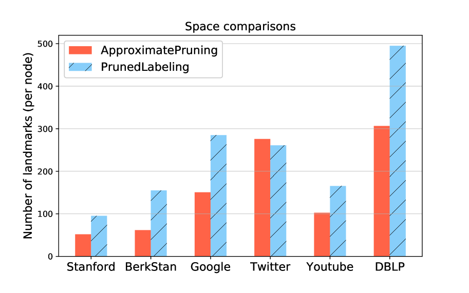
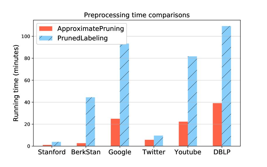
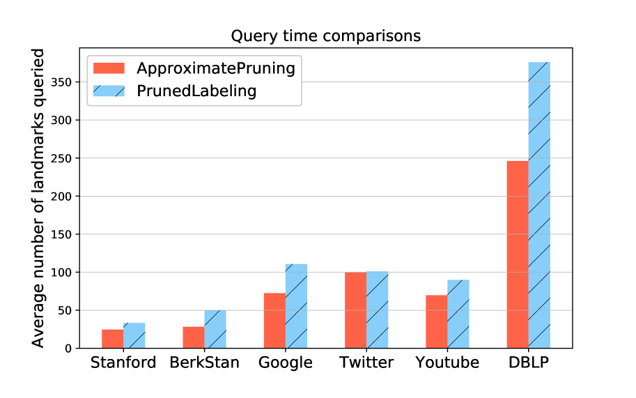
Figure 2. Comparing the efficiency of our approach to the pruned labeling algorithm.

	Stanford	BerkStan	Google	Twitter	Youtube	DBLP
Relative Average Stretch	0.37%	0.20%	0.51%	0.29%	0.33%	1.1%
Maximum Relative Stretch	21/10	10/7	8/5	4/3	4/3	7/5
Average Additive Stretch	0.046	0.030	0.060	0.014	0.018	0.075
Maximum Additive Stretch	11	3	3	1	2	2
Average Distance	12.3	14.6	11.7	4.9	5.3	6.8

Table 2. Measuring the accuracy of our approach.

Parameters: In the comparison between the pruned labeling algorithm and our approach, we order the vertices in decreasing order by the indegree plus outdegree of each vertex. Recall that there are two input parameters used in our approach, the number of global landmarks $H$ and the radiuses of local balls $\{l_{i}\}_{i=H+1}^{n}$. To tune $H$, we start with 100, then keep doubling $H$ to be 200, 400, etc. The radiuses $\{l_{i}\}_{i\geq H}$ are set to be $2$ for all graphs.

Benchmarks: For the Thorup-Zwick sketch, in the first step, $H=\sqrt{n}$ vertices are sampled uniformly at random as global landmarks. In the second step, every other vertex grows a local ball as its landmark set until it hits any of the $\sqrt{n}$ vertices. All vertices within the ball are used as landmarks. This method uses $O(n^{3/2})$ landmarks and achieves $3$-stretch in worst case. In the follow up work of Chen et al. (Chen et al., 2009), the authors show a variant which uses high degree vertices as global landmarks and observe better performance. We implement Chen et al.’s variant in our experiment, and use the $H$ vertices with the highest indegree plus outdegree as global landmarks. In the experiment, we start with $H$ equal to $\sqrt{n}$. Then we report results for $\sqrt{n}$ multiplied by $\{2,1/2,1/4,1/8\}$.

For the Das Sarma et al. sketch, first, $\log n$ sets $S_{i}$ of different sizes are sampled uniformly from the set of vertices $V$, for $0\leq i<\log n$, where the size of $S_{i}$ is $2^{i}$. Then a breadth first search is performed from $S_{i}$, so that every vertex $x\notin S_{i}$ finds its closest vertex inside $S_{i}$ in graph distance. This closest vertex is then used as a landmark for $x$. The number of landmarks used in Dar Sarma’s sketch is $n\log n$, and the worst case multiplicative stretch is $\log n$. If more accurate estimation is desired, one can repeat the same procedure multiple times and union the landmark sets together. We begin with 5 repetitions, then keep doubling it to be 10, 20 etc.

Our approach differs from the above two methods by using the idea of pruning while running BFS. This dramatically enhances performance in practice, as we shall see in our experiments.

Metrics: We measure the stretch of the estimated distances, and compute aggregated statistics over a large number of queries. For a query $(x,y)$, if $y$ is reachable from $x$, but the algorithm reports no common landmark between the landmark sets of $x$ and $y$, then we count such a mistake as a “False disconnect error.” On the other hand, if $y$ is not reachable from $x$, then it is not hard to see that our algorithm always reports correctly that $y$ is not reachable from $x$. In the experiments, we compute $\mathrm{dist}(x,y)$ using Dijkstra’s algorithm.

To measure space usage, we report the number of landmarks per node used in each algorithm as a proxy. Since the landmark sets are stored in Int to Float hash maps, the actual space usage would be eight bytes times the landmark sizes in runtime, with a constant factor overhead.

For the query time, recall that for each pair of vertices $(x,y)$, we estimate their distance by looking at the intersection of $L_{F}(x)$ and $L_{B}(y)$ and compute the minimum interconnecting distance (c.f. equation 1). To find the minimum, we iterate through the smaller landmark set. Hence the running time is $\min(\left\lvert L_{F}(x)\right\rvert,\left\lvert L_{B}(y)\right\rvert)$ multiplied by the time for a hash map lookup, which is a small fixed value in runtime. A special case is when $y\in L_{F}(x)$ or $x\in L_{B}(y)$, where only one hash map lookup is needed. We will report the number of hash map lookups as a proxy for the query time.

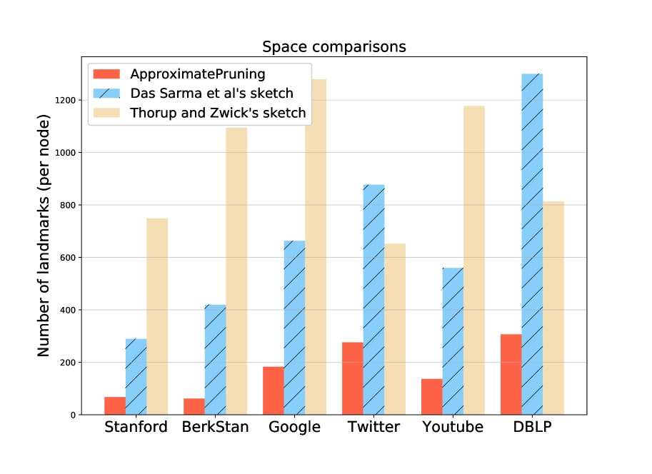
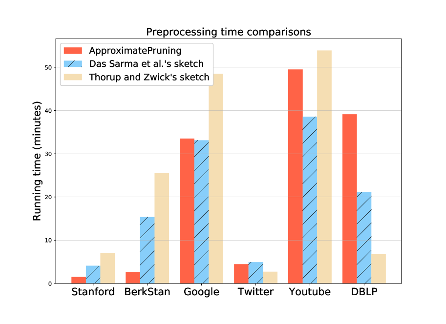
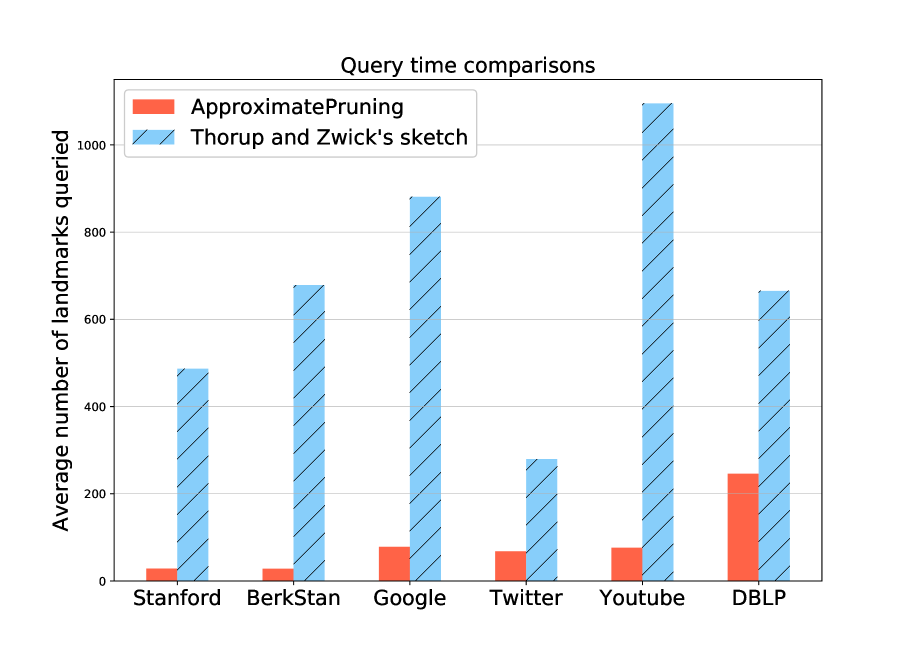
Figure 3. Comparing the efficiency of our approach to two well known distance sketches with strong theoretical guarantees.

	Stanford	BerkStan	Google	Twitter	Youtube	DBLP
DS et al. sketch	20.9%	17.2%	21.1%	11.1%	13.1%	5.4%
TZ sketch	0.30%	0.21%	0.36%	1.65%	0.03%	2.15%
Our approach	0.16%	0.20%	0.22%	0.29%	0.04%	1.1%

Table 3. Measuring the stretch for all three methods.

Youtube	${\sqrt{n}}/2$	${\sqrt{n}}/4$	${\sqrt{n}}/8$	Ours
Stretch	0.04%	0.11%	0.07%	0.04%
# Landmarks	731	648	811	137
Preprocessing	37m	31m	35m	50m

Table 4. Varying $H$ in TZ sketch.

5.2. Comparisons to Exact Methods

We report the results comparing our approach to the pruned labeling algorithm. The pruned labeling algorithm is exact. To measure the accuracy of our approach, we randomly sample $2000$ pairs of source and destination vertices. The number of global landmarks is set to be 400 for the Stanford dataset, 1600 for the DBLP dataset, and 800 for the rest of the datasets.

Figure 2 shows the preprocessing time, the number of landmarks and average query time used by both algorithms. We see that our approach reduces the number of landmarks used by 1.5-2.5x, except on the Twitter dataset. Our approach performs favorably in terms of preprocessing time and query time as well.

The accuracy of our computed estimate is shown in Table 2. We have also measured the median additive stretch, which turns out to be zero in all the experiments. To get a more concrete sense of the accuracy measures, consider the Google dataset as an example. Since the average additive stretch is $0.06$ and there are 2000 pairs of vertices, the total additive stretch is at most 120 summing over all 2000 pairs! Specifically, there can be at most 120 queries with non-zero additive stretch and for all the other queries, our approach returns the exact answer. Meanwhile, among all the datasets, we observed only one “False disconnect error” in total. It appeared in the Stanford Web graph experiment, where the true distance is 80.

5.3. Comparisons to Approximate Methods

Next we compare our approach to Das Sarma et al.’s sketch (or DS et al. sketch in short) and the variant of Thorup and Zwick’s sketch (or TZ sketch in short). Similar to the previous experiment, we sample 2000 source and destination vertices uniformly at random to measure the accuracy.

We start by setting the number of global landmarks to $\sqrt{n}$ in Thorup-Zwick sketch. To allow for a fair comparison, we tune our approach so that the relative average stretch is comparable or lower. Specifically, the Stanford, BerkStan and Twitter datasets use $H=800$, the Google and DBLP datasets use $H=1600$ and the Youtube dataset uses $H=3200$.

Figure 3 shows the number of landmarks needed in each algorithm as well as the amount of preprocessing time consumed. Overall, our approach uses much fewer landmarks than the other two algorithms. In terms of preprocessing time, our approach is comparable or faster on all datasets, except on the DBLP network. We suspect that this may be because the degree distribution of the DBLP network is flatter than the others. Hence performing the pruning procedures on a small subset of high degree vertices are less effective in such a scenario.

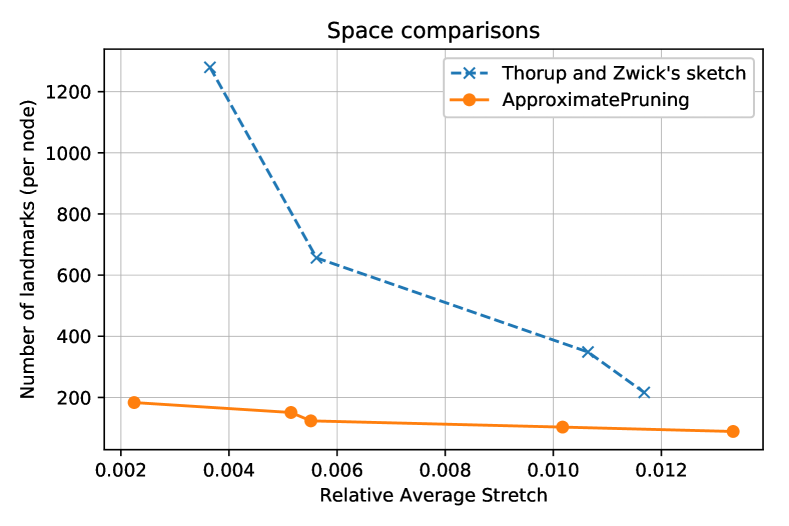
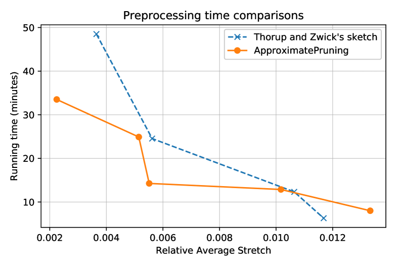
Figure 4. Varying $H$ in TZ sketch and our approach, on the Google dataset.

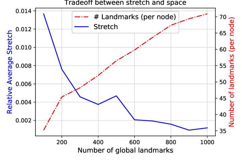
Figure 5. Tradeoff on the Stanford dataset.

We next report the relative average stretch for all three methods. As can be seen in Table 4, our approach is comparable to or slightly better than Thorup and Zwick’s sketch, but much more accurate than Das Sarma et al’s sketch. Note that the latter performed significantly worse than the other two approaches. We suspect that this may be because the sketch does not utilize the high degree vertices efficiently. Lastly, our approach performs favorably in the query time comparison as well. The query time of Das Sarma et al.’s sketch are not reported because of the worse accuracy.

Effect of parameter choice: Note that in the above experiment, for Thorup and Zwick’s sketch, we have set the number of global landmarks $H$ to be $\sqrt{n}$. In the next experiment, we vary the value of $H$ to $\sqrt{n}$ multiplied by $\{2,1/2,1/4,1/8\}$.

First, we report a detailed comparison on the Google dataset in Figure 5. Note that when $H=2\sqrt{n}$, the Thorup and Zwick’s sketch requires over 2000 landmarks per node which is significantly larger than the other values. Hence, we dropped the data point from the plot. For our approach, we double $H$ from 100 up to 1600. Overall, we can see that our approach requires fewer landmarks across different stretch levels.

Next, we report brief results on the Youtube dataset in Table 4 since the results are similar. The conclusions obtained from other datasets are qualitatively similar, and hence omitted.

5.4. More Experimental Observations

By varying the number of global landmarks used Algorithm 1, it is possible to obtain a smooth tradeoff between stretch and number of landmarks used. As an example, we present the tradeoff curve for the Stanford Web dataset in Figure 5. Here we vary the number of global landmarks used from 100 to 1000. As one would expect, the relative average stretch decreases while the number of landmarks stored increases.

6. Fundamental Limits of Landmark Sketches

This section complements our algorithm with lower bounds. We begin by showing a matching lower bound for Erdös-Rényi graphs, saying that any 2-hop cover needs to store at least $\tilde{\Omega}(n^{3/2})$ landmarks. The results imply that the parameter dependence on $n$ of our algorithm is tight for Erdös-Rényi graphs and random power law graphs with power law exponent $\beta>3$. It is worth mentioning that the results not only apply to landmark sketches, but also work for the family of labeling schemes. Recall that labeling schemes associate a labeling vector for each vertex. To answer a query for a pair of vertices $(x,y)$, only the labeling vectors of $x,y$ are accessed. We first state the lower bound for Erdös-Rényi graphs.

Theorem 1.

Let $G=(V,E)$ be an Erdös-Rényi graph where every edge is sampled with probability $p=2\log n/n$. With high probability over the randomness of $G$, any labelings which can recover all pairs distances exactly have total length at least ${\Omega}(n^{3/2}/\log^{4}n)$.

In particular, any 2-hop cover needs to store at least ${\Omega}(n^{3/2}/\log^{4}n)$ many landmarks with high probability.

For a quick overview, we divide $V$ into $\sqrt{n}$ sets of size $\sqrt{n}$ each. We will show that the total labeling length for each set of $\sqrt{n}$ vertices has to be at least $\tilde{\Omega}(n)$. By union bound over all the $\sqrt{n}$ sets, we obtain the desired conclusion. We now go into the proof details.

Proof.

Denote by $r=np$. Let $d=\lfloor\frac{\log n}{2\log(np)}\rfloor-c$, where $c$ is a fixed constant (e.g. $c=2$ suffices). Divide $V$ into groups of size $\sqrt{n}$. Clearly, there are $\sqrt{n}$ disjoint groups – let $S$ be one of them. Denote by $c_{1}$ a fixed constant which will be defined later. We argue that

(2) $$\Pr[\text{The total label length of $S$}\leq c_{1}\cdot r^{1-2c}n]\lesssim r^{1-2c}.$$

Hence by Markov’s inequality, with high probability except for $(\log n)r^{1-2c}\sqrt{n}$ groups, all the other groups will have label length at least $c_{1}\cdot r^{1-2c}n\gtrsim\tilde{\Omega}(n)$, because $r\leq 2\log n$. Hence we obtain the desired conclusion. For the rest of the proof, we focus on proving equation (2) for the group $S$.

Let $\{x_{1},x_{2},\dots,x_{\left\lvert S\right\rvert}\}$ be an arbitrary ordering of $S$. We grow the neighborhood of each vertex in $S$ one by one, up to level $d$. Denote by $G_{1}=(V_{1},E_{1})$, where $V_{1}=V$ and $E_{1}=E$. For any $i\geq 1$, if $x_{i}\in V_{i}$, then we define define $T(x_{i})$ to be the set of of vertices in $V_{i}$ whose distance is at most $d$ from $x_{i}$. Define $L(x_{i})\subseteq T(x_{i})$ to be the set of vertices in $G_{i}$ whose distance is equal to $d$ from $x_{i}$. On the other hand if $x_{i}\notin V_{i}$, then $T(x_{i})$ and $L(x_{i})$ are both empty. More formally,

$$T(x_{i}):=\begin{cases}\{y:\mathrm{dist}_{G_{i}}(x_{i},y)\leq d\},&\mbox{if }x_{i}\in V_{i}\\ \varnothing,&\mbox{otherwise.}\end{cases}$$

$$L(x_{i}):=\{y\in T(x_{i}):\mathrm{dist}_{G_{i}}(x_{i},y)=d\}$$

We then define $F_{i}=\cup_{j=1}^{i}T(x_{j})$. Denote by $G_{i+1}$ to be the induced subgraph of $G_{i}$ on the remaining vertices $V_{i+1}=V\backslash F_{i}$. We show that with high probability, a constant fraction of vertices $x_{i}\in S$ satisfy that $\left\lvert L(x_{i})\right\rvert\geq\Omega((np)^{d})$.

Lemma 2 (Martingale inequality).

In the setting of Theorem 1, with high probability, at least $\left\lvert S\right\rvert/2$ vertices $x_{i}\in S$ satisfy that $\left\lvert L(x_{i})\right\rvert\geq r^{d}/6$.

Proof.

For any $1\leq i\leq\left\lvert S\right\rvert$, consider

$$X_{i}:=\begin{cases}1&\textrm{if }x_{i}\notin V_{i},\textrm{ or }\left\lvert F_{i-1}\right\rvert>\left\lvert S\right\rvert\cdot r^{d}\log n,\textrm{or }\left\lvert L(x_{i})\right\rvert\geq r^{d}/6\\ 0&\textrm{otherwise.}\end{cases}$$

We claim that $\Pr[X_{i}=1\mid X_{1},\ldots,X_{i-1}]$ with high probability. It suffices to consider the case $x_{i}\in V_{i}$ and $\left\lvert F_{i-1}\right\rvert\leq\left\lvert S\right\rvert r^{d}\log n$. It is not hard to verify that $\left\lvert F_{i-1}\right\rvert\leq n/\log n$ by our setting of $d$. Hence the size of $V_{i}$ is at least $n(1-1/\log n)$. Note that the subgraph $G_{i}$ is still an Erdös-Rényi random graph, and the number of vertices is at least $n(1-1/\log n)$. By Fact 1c), the size of $L(x_{i})$ is at least

$$\frac{1}{2}r^{d}(1-\log^{-1}n)^{d}\geq r^{d}/6,$$

since $d\leq\log n$.

Thus by Azuma-Hoeffding inequality, $\sum_{i=1}^{\left\lvert S\right\rvert}X_{i}\geq 0.99\left\lvert S\right\rvert$ with high probability. We will show below that the contributions to $\sum_{i=1}^{\left\lvert S\right\rvert}X_{i}$ from $x_{i}\notin V_{i}$ and $\left\lvert F_{i-1}\right\rvert>\left\lvert S\right\rvert r^{d}\log n$ is less than $0.02\left\lvert S\right\rvert$. Hence by taking union bound, we obtain the desired conclusion.

First, we show that the number of $x_{i}$ such that $x_{i}\notin V_{i}$ are at most $0.01|S|$ with high probability. Note that $x_{i}\notin V_{i}$ implies that there exists some vertex $x_{j}$ with $j<i$ such that $\mathrm{dist}(x_{i},x_{j})\leq d$. On the other hand, by Fact 1,

$$\Pr[\mathrm{dist}(x,y)\leq d]\leq\frac{3r^{d}}{n},\forall x,y\in S.$$

Hence, it is not hard to verify that the expected number of vertex pairs in $S$ whose distance is at most $d$, is $O(\left\lvert S\right\rvert^{2}r^{2d}/n)\lesssim\left\lvert S\right\rvert/\log n$, by the setting of $d$. By Markov’s inequality, with probability $1-1/\log n$ only $0.01\left\lvert S\right\rvert$ vertex pairs have distance at most $d$ in $S$. Hence there exists at most $0.01\left\lvert S\right\rvert$ $i$’s such that $x_{i}\notin V_{i}$.

Secondly for all $1\leq i\leq\left\lvert S\right\rvert$, the set of vertices $T_{i}$ is a subset of $N_{d}(x_{i})$, the set of vertices within distance $d$ to $x_{i}$ on $G$. By Fact 1c), the size of $N_{d}(x_{i})$ is at most $2r^{d}$. Hence we have $\left\lvert F_{i}\right\rvert\leq 2\left\lvert S\right\rvert r^{d}$ for all $1\leq i\leq\left\lvert S\right\rvert$ with high probability. This proves the Lemma. ∎

Now we are ready to finish the proof. Given the labels of $S$, we can recover all pairwise distances in $S$. Let $\mathrm{dist}_{S}:S\times S\rightarrow\mathbb{N}$ denote the distance function restricted to $S$. Consider the following:

1. $\exists\left\lvert S\right\rvert^{2}/9$ pairs $(x_{i},x_{j})$ such that $\mathrm{dist}_{S}(x_{i},x_{j})\leq 2d+1$. We know by Fact 1 that $\Pr[\mathrm{dist}(x_{i},x_{j})\leq 2d+1]\leq 2r^{2d+1}/n$, for any $x_{i},x_{j}\in S$. Hence the expected number of pairs with distance at most $2d+1$ in $S$, is at most $2\left\lvert S\right\rvert^{2}\cdot r^{2d+1}/n\lesssim r^{1-2c}n$. By Markov’s inequality, the probability that a random graph induces any such distance function is $r^{1-2c}n/(\left\lvert S\right\rvert^{2}/8)\lesssim r^{1-2c}$.

2. The number of pairs such that $\mathrm{dist}_{S}(x_{i},x_{j})\leq 2d+1$ is at most $\left\lvert S\right\rvert^{2}/8$ in $S$. Let $A$ denote

   $$\left\{(x,y)\in S\times S\mid\mathrm{dist}(x,y)>2d+1,\mbox{ and }\left\lvert L(x)\right\rvert,\left\lvert L(y)\right\rvert\geq r^{d}/6\right\}.$$

   By Lemma 2 and our assumption for case b), the size of $A$ is at least $\binom{\left\lvert S\right\rvert/2}{2}-\left\lvert S\right\rvert^{2}/8\geq\left\lvert S\right\rvert^{2}/9.$ For any $(x,y)\in A$, $L(x)$ and $L(y)$ are clearly disjoint. Note that the event whether there exists an edge between $L(x)$ and $L(y)$ is independent, conditional on revealing the subgraph for all $x\in S$ up to distance $d$. Hence

   $$\Pr\left[\mathrm{dist}_{S}(x,y)>2d+1,~{}\forall(x,y)\in A\right]$$

   $$\leq\prod_{(x,y)\in A}\Pr\left[\mbox{there is no edge between }L(x)\mbox{ and }L(y)\right]$$

   $$\leq\prod_{(x,y)\in A}(1-p)^{\left\lvert L(x)\right\rvert\times\left\lvert L(y)\right\rvert}$$

   (because $$\left\lvert L(x)\right\rvert,\left\lvert L(y)\right\rvert\geq r^{d}/6 \leq\exp\left(-p\times\left\lvert A\right\rvert\times r^{2d}/72\right)$$)

   (because $$\left\lvert A\right\rvert\geq n/9 \leq\exp(-c_{1}r^{1-2c}n).$$)

   where $c_{1}=72\times 9$ in the last line. Denote by $\kappa=c_{1}\cdot r^{1-2c}n$. Note that the number of labelings of length (or number of bits) less than $\kappa$ is at most $2^{\kappa}$. For each labeling, the probability that it correctly gives all pairs distances is at most $\exp(-\kappa)$ by our argument above. Therefore by union bound, the probability that the total labeling length of $\left\lvert S\right\rvert$ is at most $\kappa$ is at most $2^{\kappa}\cdot\exp(\kappa)\leq r^{1-2c}$ for large enough $n$.

To recap, by combining case a) and b), we have shown that equation (2) is true. Hence the proof is complete. ∎

Extensions to $\beta>3$: It is worth mentioning that the lower bound on Erdös-Rényi graphs can be extended to random power law graphs with $\beta>3$. The proof structure is similar because the degree distribution has finite variance, hence the number of high degree vertices is small. The difference corresponds to technical modifications which deal with the neighborhood growth of random graphs with constant average degree. We state the result below and leave the proof to Appendix B.

Theorem 3.

Let $G=(V,E)$ a random power law graph with average degree $\nu>1$ and exponent $\beta>3$. With high probability over the randomness of $G$, any labelings which can recover all pairs distances exactly have total length at least $\tilde{\Omega}(n^{3/2})$.

In particular, any 2-hop cover needs to store at least $\tilde{\Omega}(n^{3/2})$ many landmarks with high probability.

Lower bounds for $\beta$ close to 2: Next we show that the parameter dependence of our algorithm is tight when $\beta$ is close to 2. Specifically, any 2-hop cover needs to store at least $\Omega(n^{3/2-\varepsilon})$ many landmarks when $\beta=2+\varepsilon$. Hence it is not possible to improve over our algorithm when $\beta$ is close to 2. Furthermore, the lower bound holds for the general family of labeling schemes as well.

Theorem 4.

Let $G=(V,E)$ a random power law graph with average degree $\nu>1$ and exponent $\beta=2+\varepsilon$ for $\varepsilon<1/2$. With high probability over the randomness of $G$, any labelings which can recover all pairs distances exactly have total length at least $\Omega(n^{3/2-\varepsilon})$.

In particular, any 2-hop cover needs to store at least $\Omega(n^{3/2-\varepsilon})$ many landmarks with high probability.

The proof is conceptually similar to Theorem 1, so we sketch the outline and leave the proof to Appendix C.

Let $S_{\mathrm{high}}$ be the set of vertices whose degrees are on the order of $\sqrt{n}$. Let $S_{\mathrm{low}}$ be a set of $\sqrt{n}$ vertices, where each vertex has weight between $\nu$ and $2\nu$. Such a set is guaranteed to exist because there are $\Theta(n)$ of them.

We first reveal all edges of $G$ other than the ones between $S_{\mathrm{high}}$. We show that at this stage, most vertices in $S_{\mathrm{low}}$ are more than 3 hops away from each other. If for some pair $(x,y)$ in $S_{\mathrm{low}}$ whose distance is larger than three, and both $x$ and $y$ connect to exactly one (but different) vertex in $S_{\mathrm{high}}$, then knowing whether $\mathrm{dist}(x,y)=3$ will reveal whether their neighbors in $S_{\mathrm{high}}$ are connected by an edge.

Based on the observation, we show that the total labeling length of $S_{\mathrm{low}}$ is at least $\tilde{\Omega}(n^{3-\beta})$. This is because the random bit between a vertex pair in $S_{\mathrm{high}}$ has entropy $\Omega(n^{2-\beta})$. Since there are $\Theta(n)$ pairs of vertices in $S_{\mathrm{high}}$, the entropy of the labelings of $S_{\mathrm{low}}$ must be $\Omega(n^{3-\beta})$ (hence, its size must also be at least $\Omega(n^{3-\beta})$). Similar to Theorem 1, this argument is applied to $\sqrt{n}$ disjoint sets of “$S_{\mathrm{low}}$”, summing up to an overall lower bound of $\Omega(n^{7/2-\beta})=\Omega(n^{3/2-\varepsilon})$.

7. Conclusions and Future Work

In this work, we presented a pruning based landmark labeling algorithm. The algorithm is evaluated on a diverse collection of networks. It demonstrates improved performances compared to the baseline approaches. We also analyzed the algorithm on random power law graphs and Erdös-Rényi  graphs. We showed upper and lower bounds on the number of landmarks used for the Erdös-Rényi  random graphs and random power law graphs.

There are several possible directions for future work. One direction is to close the gap in our upper and lower bounds for random power law graphs. We believe that any improved understanding can potentially lead to better algorithms for real world power law graphs as well. Another direction is to evaluate our approach on transportation networks, which correspond to another important domain in practice.

Acknowledgements. The authors would like to thank Fan Chung Graham, Tim Roughgarden, Amin Saberi and D. Sivakumar for useful feedback and suggestions at various stages of this work. Also, thanks to the anonymous referees for their constructive reviews. Hongyang Zhang is supported by NSF grant 1447697.

Appendix A Proof of Theorem 2: Upper Bounds for $2<\beta<3$

In this section, we present the proof of Theorem 2, which analyzes the performance of Algorithm 2 on random power law graphs. We show that Algorithm 2 outputs a 2-hop cover in Proposition 1. Then we bound the landmark set sizes in Proposition 5.

We introduce a few notations first. For a set of vertices $S\subseteq V$, let $d_{S}=\sum_{x\in S}d_{x}$ denote the sum of their degrees. Denote by $x\sim y$ if there is an edge between $x,y$. For two disjoint sets $S$ and $T$, denote by $S\sim T$ if there exists an edge between $S$ and $T$, and $S\nsim T$ if there does not exist any edge between $S$ and $T$. We use $v^{*}=\mathrm{argmax}_{x\in V}~{}p_{x}$ to denote the maximum weight vertex. For any integer $1\leq i\leq n-1$, recall that $\Gamma_{i}(x)=\{y\in V:\mathrm{dist}(x,y)=i\}$ denotes the set of vertices whose distance from $x$ is equal to $i$. And $N_{i}(x)=\{y\in V:\mathrm{dist}(x,y)\leq i\}$ denotes the set of vertices whose distance from $x$ is at most $i$. Let $\alpha_{i}(x)$ denote the number of edges between $N_{i}(x)$ and $V\backslash N_{i}(x)$. Let $\mathrm{vol}_{2}(S):=\sum_{x\in S}p_{x}^{2}$ denote the second moment of any $S\subseteq V$.

Throughout the section, we assume that $\mathbf{p}$ satisfies all the properties in Proposition 4 without loss of generality.

Proposition 1.

In the setting of Theorem 2, Algorithm 2 returns a 2-hop cover $F(\cdot)$ with high probability.

Proof.

Recall that $l_{i}$ is the radius of the local ball from $x_{i}$. Denote by $l(x_{i})=l_{i}$ for all $i\geq K+1$. Let $\Omega_{S}$ denote the set of graphs that satisfies

$$\Gamma_{l(x)}(x)=\varnothing\text{ or }\mathrm{dist}(v^{*},x)\leq l(x),\forall x\in V.$$

We argue that Algorithm 2 finds a 2-hop cover for any $G\in\Omega_{S}$, and

$$1-\mathrm{Pr}[\Omega_{S}]\leq 2/n$$

This would conclude the proof.

We first argue that Algorithm 2 is correct if $G\in\Omega_{S}$. Let $x$ and $y$ be two different vertices in $V$. If $x$ and $y$ are not reachable from each other, then clearly $F(x)\cap F(y)=\varnothing$. If $x$ and $y$ are reachable from each other, consider their distance $\mathrm{dist}(x,y)$. Note that when $\Gamma_{l(x)}(x)$ (or $\Gamma_{l(y)}(y)$) is empty, then $F(x)$ (or $F(y)$) includes the entire connected component that contains $x$ (or $y$). Therefore, $y\in F(x)$, vice versa. When none of them are empty, we know that $\mathrm{dist}(x,v^{*})\leq l(x)$ and $\mathrm{dist}(y,v^{*})\leq l(y)$ since $G\in\Omega_{S}$. We consider three cases:

• If $\mathrm{dist}(x,y)\leq l(x)+l(y)-2$, then there exists a node $z$ such that $\mathrm{dist}(x,z)\leq l(x)-1$ and $\mathrm{dist}(y,z)\leq l(y)-1$. By our construction, $z$ is in $F(x)$ and $F(y)$.

• If $\mathrm{dist}(x,y)=l(x)+l(y)-1$, then consider the two nodes $z$ and $z^{\prime}$ on one of the shortest path from $x$ to $y$, with $\mathrm{dist}(x,z)=l(x)-1$ and $\mathrm{dist}(y,z)=l(y)$. If either $d_{z}$ or $d_{z^{\prime}}$ is at least $K$, then they have been added as a landmark to every node in $V$. Otherwise, assume without loss of generality that $d_{z}\geq d_{z^{\prime}}$. Then our construction adds $z$ into $F(y)$ and clearly $z$ is also in $F(x)$, hence $z$ is a common landmark for $x$ and $y$.

• If $\mathrm{dist}(x,y)=l(x)+l(y)$, then clearly $v^{*}$ is a common landmark for $x$ and $y$.

We now bound $1-\mathrm{Pr}[\Omega_{S}]$. Clearly,

$$\ 1-\mathrm{Pr}[\Omega_{S}]$$

$$\leq \ \sum_{x\in V}\mathrm{Pr}[\Gamma_{l(x)}(x)\neq\varnothing,\mathrm{dist}(v^{*},x)>l(x)]$$

$$= \ \sum_{x\in V}\sum_{k=0}^{n-1}\mathrm{Pr}[l(x)=k+1,\Gamma_{k+1}(x)\neq\varnothing,\mathrm{dist}(v^{*},x)>k+1]$$

Note that $l(x)=k+1$ and $\Gamma_{k+1}(x)\neq\varnothing$ is the same as the event that:

• $\alpha_{i}(x)\leq\delta n^{1-\frac{1}{\beta-1}}$, for $i=0,\dots,k-1$;

• $\alpha_{k}(x)>\delta n^{1-\frac{1}{\beta-1}}$.

Hence,

$$\ \mathrm{Pr}[l(x)=k+1,\Gamma_{k+1}(x)\neq\varnothing,\mathrm{dist}(v^{*},x)>k+1]$$

$$\leq \ \mathrm{Pr}[\alpha_{k}(x)>\delta n^{1-\frac{1}{\beta-1}},\mathrm{dist}(v^{*},x)>k+1]$$

(3) $$\leq \ \mathrm{Pr}[\alpha_{k}(x)>\delta n^{1-\frac{1}{\beta-1}},\mathrm{vol}(\Gamma_{k}(x))\leq\frac{\delta n^{1-\frac{1}{\beta-1}}}{3}]$$

(4) $$+ \ \mathrm{Pr}[\mathrm{vol}(\Gamma_{k}(x))>\frac{\delta n^{1-\frac{1}{\beta-1}}}{3},\mathrm{dist}(v^{*},u)>k+1]$$

For Equation (3), consider how $\alpha_{k}(x)$ is discovered when we do the level set expansion from node $x$. Conditioned on $a=\mathrm{vol}(\Gamma_{k}(x))\leq\delta n^{1-\frac{1}{\beta-1}}/3$, $\alpha_{k}(x)$ is the sum of 0-1-2 independent random variables, with expected value less than $\delta n^{1-\frac{1}{\beta-1}}/3$. Hence by Chernoff bound, Equation (3) is at most $\exp(-\delta n^{1-\frac{1}{\beta-1}}/6)\sim o(n^{-3})$. For Equation (4), conditioned on $\mathrm{vol}(\Gamma_{k}(x))\geq\delta n^{1-\frac{1}{\beta-1}}/2$ and $v^{*}\notin N_{k}(x)$,

$$\mathrm{Pr}[v^{*}\nsim\Gamma_{k}(x)]\leq\exp\left(-\frac{\delta n^{1-\frac{1}{\beta-1}}p_{v^{*}}}{2{\mathrm{vol}(V)}}\right)\sim o(n^{-3})$$

The first inequality is because of Proposition 1. The second inequality is because ${\mathrm{vol}(V)}\sim\nu n\pm o(n)$ by Proposition 4. In summary, $1-\mathrm{Pr}[\Omega_{S}]\leq 2/n$. ∎

Next we consider the landmark set sizes. There are three parts in each landmark set: (1) the heavy nodes whose degrees are at least $K$; (2) all the level sets before the last layer; (3) the last layer that we carefully constructed. It’s not hard to bound the first part, since the degree of a node is concentrated near its weight, and it is not hard to show that the number of vertices whose weight is $\Omega(K)$ is ${\textsc{O}}(nK^{1-\beta})$. The second part can be bounded by the maximum number of layers, which is at most $O(\log n)$, the diameter of $G$. For the third part, the idea is that before adding all the nodes on the boundary layer, we already have a $(+1)$-stretch scheme. Therefore, for a given vertex $x$, it is enough if we only add neighbors whose degree is bigger than themselves. This reduces the amount of vertices from $d_{x}$ to ${\textsc{O}}(d_{x}^{3-\beta})$, where $d_{x}$ denotes the degree of any vertex $x\in V$.

We first show that the volume of all the level sets is at most $\textsc{O}(\delta n^{1-\frac{1}{\beta-1}})$ before the boundary layer in Proposition 2 and 3. For the rest of the section, denote by $\alpha_{k}=\alpha_{k}(x)$ for any $0\leq k\leq n-1$, unless there is any ambiguity on the vertex we are considering. Recall that $\alpha_{k}$ denotes the number of edges between $\Gamma_{k}(x)$ and $V\backslash N_{k-1}(x)$.

Proposition 2.

Let $x$ be a fixed node. Let $k\lesssim\log n$. Let $\Omega_{k}$ denote the set of graphs such that

$$\mathrm{vol}(\Gamma_{i}(x))<4\delta n^{1-\frac{1}{\beta-1}},\text{ for any }0\leq i\leq k-1,$$

and

$$\mathrm{vol}(\Gamma_{k}(x))>4\delta n^{1-\frac{1}{\beta-1}}.$$

Then $\mathrm{Pr}[\alpha_{k}\leq\delta n^{1-\frac{1}{\beta-1}}\mid\Omega_{k}]\leq n^{-2}$.

Proof.

Let $a=\mathrm{vol}(\Gamma_{k}(x))$ and $b=\mathrm{vol}(N_{k-1}(x))$. Conditioned on $\Omega_{k}$,

$$a>4\delta n^{1-\frac{1}{\beta-1}}\text{ and }b\leq 4k\delta n^{1-\frac{1}{\beta-1}}.$$

Clearly, the random variable $\alpha_{k}$ is the sum of independent 0-1 random variables. Let $\mu$ denote its expected value. For each $y\in\Gamma_{k}(x)$, we know that $p_{y}\leq a=O(\sqrt{n})$. Let $\mu_{y}$ denote the expected number of edges between $y$ and $V\backslash N_{k-1}(x)$, then

$$\mu_{y} =\sum_{z:z\neq y\land z\notin N_{k-1}(x)}\min(\frac{p_{y}p_{z}}{\mathrm{vol}(V)},1)\mathbbm{1}_{p_{z}\leq\sqrt{n}}$$

$$\geq p_{y}(1-\frac{b+\sum_{z\in V}p_{z}\mathbbm{1}_{p_{z}\geq\sqrt{n}}}{\mathrm{vol}(V)})=p_{y}(1-\kappa(n))$$

because of Proposition 4. And $\mu=\sum_{y\in\Gamma_{k}(x)}\mu_{y}=(1-o(1))a.$ Let $c=\frac{\mu}{\delta n^{1-\frac{1}{\beta-1}}}\geq 2-o(1)$. By Chernoff bound,

$$\mathrm{Pr}[\alpha_{k}\leq\delta n^{1-\frac{1}{\beta-1}}\mid\Omega_{k}]\leq\exp(-\frac{(c-1)^{2}\delta n^{1-\frac{1}{\beta-1}}}{4})\sim o(n^{-2})$$

∎

Proposition 3.

Let $x$ be a fixed vertex. Let $0\leq k\lesssim\log n$. Denote by $\Omega^{*}_{k}$ the set of graphs such that

$$\alpha_{i}\leq\delta n^{1-\frac{1}{\beta-1}},\text{ for any }0\leq i\leq k$$

Then $\mathrm{Pr}[\mathrm{vol}(\Gamma_{k}(x))>4\delta n^{1-\frac{1}{\beta-1}},\Omega^{*}_{k}]\leq(k+1)n^{-2}$.

Proof.

When $k=0$, the claim is proved by Proposition 2. When $k\geq 1$, we will repeatedly apply Proposition 2 to prove the statement. For any values of $i$ smaller than or equal to $k$, let $S_{i}\subset\Omega^{*}_{k}$ denote the set of graphs that also satisfy: (1) $\mathrm{vol}(\Gamma_{j}(x))\leq 4\delta n^{1-\frac{1}{\beta-1}}$, for any $0\leq j\leq i-1$; (2) $\mathrm{vol}(\Gamma_{k}(x))>4\delta n^{1-\frac{1}{\beta-1}}$. We show that $\mathrm{Pr}[S_{i}]-\mathrm{Pr}[S_{i+1}]\leq n^{-2}$ if $0\leq i\leq k-1$, and $\mathrm{Pr}[S_{k}]\leq n^{-2}$. The conclusion follows from the two claims.

For the first part,

$$\mathrm{Pr}[S_{i}]-\mathrm{Pr}[S_{i+1}] =\mathrm{Pr}[\mathrm{vol}(\Gamma_{i}(x))>4\delta n^{1-\frac{1}{\beta-1}},S_{i}]$$

$$\leq\mathrm{Pr}[\Omega_{i},\alpha_{i}\leq\delta n^{1-\frac{1}{\beta-1}}]\leq n^{-2}$$

The first inequality is because if $G\in S_{i}$ and $G$ satisfies $\mathrm{vol}(\Gamma_{i}(x))>4\delta n^{1-\frac{1}{\beta-1}}$, then $G\in\Omega_{i}$. Also $\alpha_{i}\leq\delta n^{1-\frac{1}{\beta-1}}$ since $G\in S_{i}\subset\Omega^{*}_{k}$. The second inequality is because of Proposition 2. The other part can be proved similarly and we omit the details. ∎

The following proposition helps us control the number of landmarks added in the bottom layer of the local ball.

Proposition 4.

Let $x$ be a fixed node with weight $p_{x}\leq 2K$. Denote by

$$S_{x}=\{y\in N(x):d_{x}\leq d_{y}\text{ and }d_{y}\leq K\}$$

and let $\hat{d}_{x}=|S_{x}|$. Then

$$\mathrm{Pr}[\hat{d}_{x}\geq\max(c_{1}{p_{x}}^{3-\beta},c_{2}\log n)]\leq n^{-3}$$

where $c_{1}=\frac{192Z}{\nu(\beta-2)}$ and $c_{2}=130$.

Proof.

When $p_{x}\leq c_{2}\log n/2$,

$$\mathrm{Pr}[\hat{d}_{x}\geq c_{2}\log n]\leq\mathrm{Pr}[d_{x}\geq c_{2}\log n]\leq o(n^{-3})$$

Now suppose that $p_{x}>c_{2}\log n/2$. Consider any vertex $y$ whose weight is at most $p_{x}/8$. Then

$$\mathrm{Pr}[d_{y}\geq d_{x}] \leq\mathrm{Pr}[d_{y}\geq p_{x}/4]+\mathrm{Pr}[d_{x}<p_{x}/4]\sim o(n^{-4})$$

The second inequality is because of Proposition 2. Hence $y$ is not in $S_{x}$.
Now if $p_{y}\geq 2K$, then $\mathrm{Pr}[d_{y}\leq K]\leq\sim o(n^{-4})$. Hence $y$ is also not in $S_{x}$. Lastly, let $X$ denote the set of vertices whose weight is between $[\frac{p_{x}}{8},2K]$ and who is connected to $x$. We have

$$\mathbb{E}[X] =\sum_{y\in V\setminus\{x\}:p_{x}/8\leq p_{y}\leq 2K}\frac{p_{x}p_{y}}{\mathrm{vol}(V)}$$

$$\leq\frac{4p_{x}}{{\mathrm{vol}(V)}}\max(\frac{8Z}{\beta-1}n{p_{x}}^{2-\beta},\sqrt{n}\log n)$$

$$\leq\max(c_{1}{p_{x}}^{3-\beta},c_{2}\log n)/3$$

The first inequality is because of Proposition 4. The second inequality is because ${\mathrm{vol}(V)}=\nu n+o(n)$ by Proposition 4, and $p_{x}\leq 2K\leq 2\sqrt{n}$. From here it is not hard to obtain that $\mathrm{Pr}[|X|\leq\max(c_{1}{p_{x}}^{3-\beta},c_{2}\log n)]\sim o(n^{-3})$. ∎

Now we are ready to bound the output size of Algorithm 2 with the following Proposition.

Proposition 5.

In the setting of Theorem 2, we have that the following holds with high probability:

• $|F(x)|\lesssim\max\left(n^{\frac{\beta-2}{\beta-1}},n^{\frac{3-\beta}{4-\beta}}\right)\cdot\log^{3}n$ for all $x\in V$;

• The algorithm terminates in time $O\left(\max\left(n^{1+\frac{\beta-2}{\beta-1}},n^{1+\frac{3-\beta}{4-\beta}}\right)\cdot\log^{3}n\right)$.

Proof.

We first bound the number of nodes in $H$. By Proposition 3, with probability $1-n^{-1}$

$$|H|\lesssim nK^{1-\beta}\lesssim O(n^{1-\min(\frac{1}{\beta-1},\frac{1}{4-\beta})})$$

Secondly, we bound the number of landmarks added before reaching the boundary layer. For any vertex $x$, with $i=0,\dots,l(x)-2$, $|\Gamma_{i}(x)|\leq\alpha_{i}(x)=O(\delta n^{1-\frac{1}{\beta-1}})$. Since $l(x)\leq O(\log n)$, the total landmarks for these layers are at most $O(n^{1-\frac{1}{\beta-1}}\log^{3}n)$. The rest of the proof will bound the number of landmarks on the boundary layer with depth $l(x)-1$.
Denote by

$$\pi_{k}(x)=\sum_{y\in\Gamma_{k}(x)}\hat{d}_{y}\mathbbm{1}_{d_{y}\leq K}\quad\text{ for }x\in V,0\leq k\leq n-1$$

Hence $\pi_{l(x)-1}(x)$ gives the number of landmarks added on the boundary layer.
Set $c_{3}=\frac{3Z}{\left\lvert 2\beta-5\right\rvert}\max(x_{\min}^{5-2\beta},1)$, $\psi=12c_{3}\delta n^{1-\min(\frac{1}{\beta-1},\frac{1}{4-\beta})}$, and $\Delta=\max(c_{1}\psi,c_{2}\delta n^{1-\frac{1}{\beta-1}}\log n)$, where $c_{1}$ and $c_{2}$ are defined in Proposition 4. We show that $\pi_{l(x)-1}(x)\leq\Delta$ with probability $1-n^{-2}$ for the rest of the proof — our conclusion follows by taking union bound over $x\in V$ and $1\leq l(x)\leq O(\log n)$.

When $l(x)=1$, $\pi_{0}(x)=d_{x}\leq K\leq\Delta$. When $l(x)=k+1\geq 2$, we know that $G\in\Omega^{*}_{k-1}$. Hence by Proposition 3, $\mathrm{vol}(\Gamma_{k-1}(x))\leq 4\delta n^{1-\frac{1}{\beta-1}}$ with high probability. More concretly,

$$\ \mathrm{Pr}[l(x)=k+1,\pi_{k}(x)\geq\Delta]$$

(5) $$\leq \ (k+1)n^{-2}+\Pr[l(x)=k+1,\mathrm{vol}(\Gamma_{k-1}(x))\leq 4\delta n^{1-\frac{1}{\beta-1}},\pi_{k}(x)\geq\Delta]$$

Denote by

$$w_{k}=\sum_{y\in\Gamma_{k}(x)}{p_{y}}^{3-\beta}\mathbbm{1}_{p_{y}\leq 2K}.$$

Conditional on $a=\mathrm{vol}(\Gamma_{k-1}(x))\leq 4\delta n^{1-\frac{1}{\beta-1}}$, we show that $w_{k}\leq\psi$ with high probability. Denote by $\Omega_{w}$ the set of graphs satisfying $a\leq 4\delta n^{1-\frac{1}{\beta-1}}$. Conditioned on $\Omega_{w}$, $w_{k}$ is the sum of independent random variables that are all bounded in $[0,(2K)^{3-\beta}]$. Hence

$$\mathbb{E}[w_{k}] =\sum_{y\notin N_{k-1}(x)}\mathrm{Pr}[y\sim N_{k-1}(x)]{p_{y}}^{3-\beta}\mathbbm{1}_{p_{y}\leq 2K}$$

$$\leq\frac{a}{\mathrm{vol}(V)}(\sum_{y\notin N_{k-1}(x)}{p_{y}}^{4-\beta}\mathbbm{1}_{p_{y}\leq 2K})$$ (by Proposition 1)

$$\leq\frac{a}{\mathrm{vol}(V)}(\sum_{y\in V}{p_{y}}^{4-\beta}\mathbbm{1}_{p_{y}\leq 2K})$$

$$\leq\frac{a\phi(K)n}{{\mathrm{vol}(V)}}$$ (by Proposition 4)

$$\lesssim\frac{a\phi(K)}{\nu} {\mathrm{vol}(V)}=\nu n\pm o(n)$$ ( by Proposition 4)

$$\leq\frac{\psi}{3}.$$

The last line follows by $a\leq 4\delta n^{1-\frac{1}{\beta-1}}$ and $\phi(K)n^{1-\frac{1}{\beta-1}}\leq c_{2}n^{1-\min(\frac{1}{\beta-1},\frac{1}{4-\beta})}$. Now we apply Chernoff bound on $w_{k}$,

$$\mathrm{Pr}[w_{k}>\psi\mid\Omega_{w}]\leq\exp(-\frac{\psi}{4(2K)^{3-\beta}})\sim o(n^{-2})$$

because when $2.5\leq\beta\leq 3$,

$$\frac{\psi}{K^{3-\beta}}=\Theta(n^{1-\frac{1}{\beta-1}-\frac{3-\beta}{2}})=\Theta(n^{\frac{(\beta-1)^{2}-2}{2(\beta-1)}})$$

And when $2<\beta<2.5$,

$$\frac{\psi}{K^{3-\beta}}=\Theta(n^{\frac{(3-\beta)(\beta-2)}{(4-\beta)(\beta-1)}})$$

Hence the second part in Equation (5) is bounded by $o(n^{-2})$ plus

$$\ \Pr[l(x)=k+1,\mathrm{vol}(\Gamma_{k-1}(x))\leq 4\delta n^{1-\frac{1}{\beta-1}},w_{k}\leq\psi,\pi_{k}(x)\geq\Delta]$$

$$\leq \ \mathrm{Pr}[w_{k}\leq\psi,\alpha_{k-1}\leq\delta n^{1-\frac{1}{\beta-1}},\pi_{k}(x)\geq\Delta]$$

$$\leq \ \mathrm{Pr}[w_{k}\leq\psi,|\Gamma_{k}(x)|\leq\delta n^{1-\frac{1}{\beta-1}},\pi_{k}(x)\geq\Delta]$$

In the reminder of the proof we show the above Equation is at most $n^{-2}$. Denote by

$$\pi^{\prime}_{k}(x)=\sum_{y\in\Gamma_{k}(x)}\hat{d}_{y}\mathbbm{1}_{p_{y}\leq 2K}$$

By Proposition 2, $\mathrm{Pr}[d_{y}\leq K\mid p_{y}>2K]\leq\exp(-K/8)\sim o(n^{-3})$ for any $y\in V$. Hence $\pi^{\prime}_{k}(x)=\pi_{k}(x)$ with probability at least $1-o(n^{-2})$. Lastly, we have

$$\mathrm{Pr}[w_{k}\leq\psi,|\Gamma_{k}(x)|\leq\delta n^{1-\frac{1}{\beta-1}},\pi^{\prime}_{k}(x)\geq\Delta]\leq n^{-2}$$

Otherwise, there exists a vertex $y\in\Gamma_{k}(x)$ such that $p_{y}\leq 2K$ and $\hat{d}_{y}\geq\max(c_{1}{p_{y}}^{3-\beta},c_{2}\log n)$, because $\Delta\geq\max(c_{1}\psi,c_{2}\delta n^{1-\frac{1}{\beta-1}}\log n)$. This happens with probability at most $n^{-2}$, by taking union bound over every vertex with Proposition 4. ∎

Appendix B Proof of Theorem 3: Lower Bounds for $\beta>3$

In this section, we present lower bounds for distance labelings on random power law graphs when $\beta>3$. We will consider lower bounds for labeling schemes that can estimate all pairs distances up to $K\leq\log n/\log r$, where $r$ is equal to $\frac{\mathrm{vol}_{2}(V)}{\mathrm{vol}(V)}$. More formally, we say that a labeling scheme is $K$-accurate if for any $x,y\in V$:

• if $\mathrm{dist}(x,y)\leq K$, then the labeling scheme returns the exact distance $\mathrm{dist}(x,y)$.

• if $\mathrm{dist}(x,y)>K$, then the labeling scheme returns “$\mathrm{dist}(x,y)>K$”.

Let $d$ be an integer smaller than $K/2$.

We may assume without loss of generality for every $x$, the label of $x$ stores the distances between $x$ and all vertices in $N_{d}(x)$. This is because the lower bound we are aiming at is larger than the size of $N_{d}(x)$, we can always afford to store them. From the labels of $x,y$, either we see a non-empty intersection between $N_{d}(x)$ and $N_{d}(y)$, which determines their distance; or the two sets are disjoint, in which case we are certain that $\mathrm{dist}(x,y)\geq 2d+1$. In a random graph, the event that $\mathrm{dist}(x,y)>2d+1$, conditioned on $\mathrm{dist}(x,y)\geq 2d+1$ and $N_{d}(x)$ and $N_{d}(y)$ are disjoint, happens with probability

$$\Theta\left({\frac{\mathrm{vol}(\Gamma_{d}(x))\cdot\mathrm{vol}(\Gamma_{d}(y))}{\mathrm{vol}(V)}}\right),$$

by Proposition 1, assuming that $\mathrm{vol}(\Gamma_{d}(x))\mathrm{vol}(\Gamma_{d}(y))\leq o(\mathrm{vol}(V))$. Note that this probability gives us a lower bound on the entropy of the event $\mathbf{1}_{\mathrm{dist}(x,y)>2d+1}$. Since the labels of $x$ and $y$ determine their distance, if we can find a large number of pairwise independent pairs $(x,y)$ such that the entropy of $\mathbf{1}_{\mathrm{dist}(x,y)>2d+1}$ is large (e.g. $1/\mathrm{poly}\log(n)$ suffices), then we obtain a lower bound on the total labeling size.

Our discussion so far suggests the following three step proof plan.

• Pick a parameter $d$ and a maximal set of vertices $S$, such that by “growing” the local neighborhood of $S$ up to $d$, $N_{d}(x),N_{d}(y)$ are disjoint/independent and $\Gamma_{d}(x),\Gamma_{d}(x)$ have large volume, for certain pairs of $x,y\in S$.

• Use the labels of $S$ to infer whether there are edges between $\Gamma_{d}(x)$ and $\Gamma_{d}(y)$, for certain pairs of $x,y$. Obtain a lower bound on the total label length of $S$ via entropic arguments.

• Partition the graph into disjoint groups of size $\left\lvert S\right\rvert$. Apply step b) for each group.

Clearly, given any two vertices, their neighborhood growth are correlated with each other. However, one would expect that the correlation is small, so long as the volume of the neighborhood has not reached $\Theta(\sqrt{n})$. To leverage this observation, We describe an iterative process to grow the neighborhood of $S$ up to distance $d$. For simplicity, we assume that $S=\{x_{1},x_{2},\ldots\}$ only consists of vertices whose weight are all within $[\nu,2\nu]$. The motivation is to find disjoint sets $L(x_{i})$ for each $x_{i}$, such that $L(x_{i})$ is almost as large as $\Gamma_{d}(x_{i})$, and if $\mathrm{dist}(x_{i},x_{j})>2d+1$, then there is no edge between $L(x_{i})$ and $L(x_{j})$.

The iterative process: Denote by $G_{1}=(V_{1},E_{1})$, where $V_{1}=V$ and $E_{1}=E$. For any $i\geq 1$, define $T(x_{i})$ to be the set of of vertices in $G_{i}$ whose distance is at most $d$ from $x_{i}$. Define $L(x_{i})$ to be the set of vertices in $G_{i}$ whose distance is equal to $d$ from $x_{i}$. More formally,

$$T(x_{i}):=\begin{cases}\{y:\mathrm{dist}_{G_{i}}(x_{i},y)\leq d\},&\mbox{if }x_{i}\in V_{i}\\ \varnothing,&\mbox{otherwise.}\end{cases}$$

$$L(x_{i}):=\{y\in T(x_{i}):\mathrm{dist}_{G_{i}}(x_{i},y)=d\}$$

We then define $F_{i}=F_{i-1}\,\cup\,T(x_{i})$ ($F_{0}:=\varnothing$ by default). Denote by $G_{i+1}$ to be the induced subgraph of $G_{i}$ on the remaining vertices $V_{i+1}=V\backslash F_{i}$.

We note that in the above iterative process, the neighborhood growth of $x_{i}$ only depends on the degree sequence of $V_{i}$. We show that under certain conditions, with high probability, a constant fraction of vertices $x\in S$ satisfy that $\mathrm{vol}(L(x))\geq\Omega(r^{d})$.

Lemma 1 (Martingale inequality).

Let $r=\frac{\mathrm{vol}_{2}(V)}{\mathrm{vol}(V)}$. Let $d$ be an integer and $S\subseteq V$ be a set of vertices whose weight are all within $[\nu,2\nu]$ and $\left\lvert S\right\rvert\leq o(\frac{\mathrm{vol}(V)}{\nu^{2}r^{d-1}})$. Assume that

• $\Pr[\mathrm{vol}(L(x_{i}))\geq\nu\cdot r^{d}\mid\mathrm{vol}(F_{i-1})\leq\left\lvert S\right\rvert\nu\cdot r^{d}\log n,x_{i}\in V_{i}]\geq\Omega(1)$, for all $1\leq i\leq\left\lvert S\right\rvert$;

• $\mathop{\mathbb{E}}[\mathrm{vol}(N_{d}(x))]\lesssim\nu\cdot r^{d}$, for all $x\in S$;

• $\Pr[\mathrm{dist}(x,y)\leq d]\lesssim\frac{\nu^{2}\cdot r^{d-1}}{\mathrm{vol}(V)}$, for all $x,y\in S$.

Then with high probability, at least $c_{1}\left\lvert S\right\rvert$ vertices $x\in S$ satisfy that $\mathrm{vol}(L(x))\geq\Omega(\nu r^{d})$, for a certain fixed constant $c_{1}$.

Proof.

Consider the following random variable, for any $1\leq i\leq\left\lvert S\right\rvert$.

$$X_{i}:=\begin{cases}1&\textrm{if }x_{i}\notin V_{i},\textrm{ or }\mathrm{vol}(F_{i-1})>\left\lvert S\right\rvert\nu\cdot r^{d}\log n,\textrm{or }\mathrm{vol}(L(x_{i}))\geq\Omega(r^{d})\\ 0&\textrm{otherwise.}\end{cases}$$

We have $\Pr[X_{i}=1\mid X_{1},\ldots,X_{i-1}]\geq\Omega(1)$ by Assumption i). Thus by Azuma-Hoeffding inequality, $\sum_{i=1}^{\left\lvert S\right\rvert}X_{i}\geq\Omega(\left\lvert S\right\rvert)$ with high probability. We will show below that the contributions to $\sum_{i=1}^{\left\lvert S\right\rvert}X_{i}$ from the first two predicates is $o(\left\lvert S\right\rvert)$. Hence by taking union bound, we obtain the desired conclusion.

First, we show that the number of $x_{i}$ such that $x_{i}\notin V_{i}$ is $o(|S|)$ with high probability. Note that $x_{i}\notin V_{i}$ implies that there exists some vertex $j<i$ such that $\mathrm{dist}(x_{i},x_{j})\leq d$. On the other hand, for any two vertices $x,y\in S$, $\Pr[\mathrm{dist}(x,y)\leq d]\leq O(\nu^{2}\cdot r^{d-1}/{\mathrm{vol}(V)})$, by Assumption iii). Hence, the expected number of vertex pairs in $S$ whose distance is at most $d$, is $O(\left\lvert S\right\rvert^{2}\nu^{2}\cdot r^{d-1}/{\mathrm{vol}(V)})\leq o(\left\lvert S\right\rvert)$, by the assumption on the size of $S$. By Markov’s inequality, with high probability only $o(\left\lvert S\right\rvert)$ vertex pairs have distance at most $d$ in $S$. Hence there exists at most $o(\left\lvert S\right\rvert)$ $i$’s such that $x_{i}\notin V_{i}$.

Secondly, for all $1\leq i\leq\left\lvert S\right\rvert$, $\mathrm{vol}(F_{i})\leq\left\lvert S\right\rvert\nu\cdot r^{d}\log n$ with high probability. This is because the set of vertices $T_{i}$ is a subset of $N_{d}(x_{i})$, the set of vertices within distance $d$ to $x_{i}$ on $G$. Thus, by Assumption ii), we have

$$\mathop{\mathbb{E}}[\mathrm{vol}(T_{i})]\leq\mathop{\mathbb{E}}[\mathrm{vol}(N_{d}(x_{i}))]\leq O(\nu r^{d}).$$

And the expected volume of ${F}_{i}$ is at most

$$O(i\cdot\nu\cdot r^{d})\lesssim\left\lvert S\right\rvert\nu\cdot r^{d},$$

Hence by Markov’s inequality, the probability that $\mathrm{vol}(N_{d}(S))>\left\lvert S\right\rvert\nu\cdot r^{d}\log n$ is at most $\log^{-1}n$. This proves the lemma. ∎

We first introduce the following proposition for growing the neighborhood of vertices.

Proposition 2 (Iterative neighborhood growth).

Let $c=(3+1/\gamma)\log_{r}\log n$ and $d=K/2-c$. Let $S$ be a set of $n/r^{K/2}$ vertices whose weight are all within $[\nu,2\nu]$. With high probability, at least $c_{1}\left\lvert S\right\rvert$ vertices in $S$ satisfy that $\mathrm{vol}(L(x))\geq\Omega(r^{d})$.

Proof.

It’s easy to verify that $\left\lvert S\right\rvert\cdot{\nu^{2}r^{d-1}}\leq n/r^{c}\leq o(n)$. It suffices to verify the assumptions required in Lemma 1. Note that Assumption ii) and iii) simply follows from Proposition 5. Hence it suffices to verify Assumption i). Note that the subgraph $G_{i}$ can be viewed as a random graph sampled from Chung-Lu model over $V_{i}$. By setting

$$p_{y}^{(i)}=p_{y}\cdot\left(1-\frac{\mathrm{vol}(F_{i-1})}{\mathrm{vol}(V)}\right),~{}\forall\,y\in V_{i},$$

we have that $\forall\,y,z\in V_{i}$

$$\Pr[y\sim z]=\frac{p_{y}\cdot p_{z}}{\mathrm{vol}(V)}=\frac{p_{y}^{(i)}\cdot p_{z}^{(i)}}{\left(1-\frac{\mathrm{vol}(F_{i-1})}{\mathrm{vol}(V)}\right)\cdot\mathrm{vol}(V_{i})}=\frac{p_{y}^{(i)}\cdot p_{z}^{(i)}}{\sum_{x\in V_{i}}p_{x}^{(i)}}.$$

Hence we see that $G_{i}$ is equivalent to a random graph drawn from degree sequence $\mathbf{p}^{i}$. Denote by $r_{i}:=\frac{\mathrm{vol}_{2}(V_{i})}{\mathrm{vol}(V)}$ the growth rate on $G_{i}$. When $\mathrm{vol}(F_{i-1})\leq n/\log^{2+1/\gamma}n$, by Hölder’s inequality,

$$\mathrm{vol}_{2}(F_{i-1})\leq\mathrm{vol}(F_{i-1})^{\frac{\gamma}{1+\gamma}}\cdot O(n^{\frac{1}{1+\gamma}})\leq o(n/\log n).$$

by straightforward calculation. Hence $r_{i}$ is a constant strictly greater than $1$. By Proposition 5, with constant probability $\mathrm{vol}(L_{i})\geq\Omega(r_{i}^{d})\geq\Omega(r^{d})$, because

$$\left(\frac{\mathrm{vol}(V)}{\mathrm{vol}(V_{i})}\right)^{d}\lesssim(1+\log^{-2-\frac{1}{\gamma}}n)^{O(\log n)}\lesssim 1+\log^{-1-\frac{1}{\gamma}}n.$$

Since the vertices at distance $d$ from $x_{i}$ in $G_{i}$ is exactly $L_{i}$, we have verified that Assumption i) is correct. ∎

Now we are ready to prove Theorem 3.

Proof of Theorem 3.

Set $K=\lceil\log n/\log(np)\rceil+1$, i.e. slightly larger than the average distance of $G$. We know that there are $\Theta(n)$ vertices whose weights are between $[\nu,2\nu]$, by an averaging argument. Divide them into groups of size $n/r^{K/2}$. Clearly, there are $\Theta(r^{K/2})=\Theta(\sqrt{n})$ disjoint groups. Denote by $c_{2}$ a small fixed value (e.g. $1/\log\log n$ suffices). We will argue that for each group $S$,

(6) $$\Pr[\text{The total label length of $S$}\leq c_{2}\cdot r^{-2c}n]\leq o(1).$$

Hence by Markov’s inequality, except for $o(n/r^{K/2})$ groups, all the other groups will have label size at least $\tilde{\Omega}(n)$. For the rest of the proof, we focus on an individual group $S$.

Given the labels of $S$, we can recover the pairwise distances less than $K$ for all vertex pairs in $S$. Let $\mathrm{dist}_{S}:S\cdot S\rightarrow\mathbb{N}$ denote the distance function restricted to all pairs in $S$. Consider the following two cases:

1. $\exists c_{1}^{2}\cdot\left\lvert S\right\rvert^{2}/4$ pairs $(x_{i},x_{j})$ such that $\mathrm{dist}_{S}(x_{i},x_{j})\leq 2d+1$. By Lemma 5, we know that $\Pr[\mathrm{dist}(x_{i},x_{j})\leq 2d+1]=O(r^{2d}/n)$, for any $x_{i},x_{j}\in S$. Hence the expected number of pairs with distance at most $2d+1$ in $S$, is at most $O(\left\lvert S\right\rvert^{2}\cdot r^{2d}/n)\lesssim r^{-2c}$. Hence by Markov’s inequality, the probability that a random graph induces any such distance function is $o(1)$.

2. The number of pairs such that $\mathrm{dist}_{S}(x_{i},x_{j})\leq 2d+1$ is at most $c_{1}^{2}\cdot\left\lvert S\right\rvert^{2}/4$ in $S$. Let

   $$A=\{(x,y)\in S\cdot S\mid\mathrm{dist}(x,y)>2d+1,\mbox{ and }\mathrm{vol}(L(x)),\mathrm{vol}(L(y))\geq\Omega(r^{d})\}.$$

   By Lemma 1, the size of $A$ is at least

   $$\binom{c_{1}\left\lvert S\right\rvert}{2}-c_{1}^{2}\left\lvert S\right\rvert^{2}/4\geq c_{1}^{2}\left\lvert S\right\rvert^{2}/5.$$

   For any $(x,y)\in A$, $L(x)$ and $L(y)$ are clearly disjoint. Conditional on $\{T(x)\}$ for all $x\in S$, the probability of the existences of edges between $L_{i}$ and $L_{j}$ are unaffected.

   $$\Pr\left[\mathrm{dist}_{S}(x,y)>2d+1,~{}\forall(x,y)\in A\mid\{T_{i}\}_{i=1}^{\left\lvert S\right\rvert}\right]$$

   $$\leq\prod_{(x,y)\in A}\Pr\left[L(x)\not\sim L(y)\mid L(x)\cap L(y)=\varnothing,\mbox{ and }\mathrm{vol}(L(x)),\mathrm{vol}(L(y))\geq\Omega(r^{d})\right]$$

   ((by Proposition 1)) $$\leq\prod_{(x,y)\in A}\exp\left(-\frac{\mathrm{vol}(L(x))\mathrm{vol}(L(y))}{\mathrm{vol}(V)}\right)$$

   $$\leq\exp\left(-\Omega\left(\frac{r^{2d}}{n}\right)\right)^{c_{1}^{2}\left\lvert S\right\rvert^{2}/5}$$

   $$\leq\exp(-\Omega(r^{-2c}n)).$$

   Note that the number of labeling of size less than $c_{2}\cdot r^{-2c}n$ is at most $2^{c_{2}\cdot r^{-2c}n}$. Therefore by union bound, the probability that the total label size of $\left\lvert S\right\rvert$ is at most $c_{2}\cdot r^{-2c}n$ is at most:

   $$2^{c_{2}\cdot r^{-2c}n}\cdot\exp(-\Omega(r^{-2c}n))\leq o(1).$$

By taking a union bound over cases a) and b), we have shown that Equation (6) is true. Hence the proof is complete. ∎

Appendix C Proof of Theorem 4: Lower Bounds for $2<\beta<3$

In this section, we prove the lower bound on distance labelings when $2<\beta<3$.

Proof of Theorem 4.

First, one can easily verify that there are $\Theta(n)$ vertices with weight between $[\nu,2\nu]$ with high probability. We divide them into $\Theta(\sqrt{n})$ groups of size $\sqrt{n}$ each. We will show that for each group, its total labeling length is at least $cn^{3-\beta}$ with high probability, where $c$ is a fixed constant. Hence in expectation, except for at most $o(\sqrt{n})$ groups, the total labeling length for all other groups is at least $\Omega(n^{3-\beta})$. Then by Markov’s inequality, among the $\Theta(\sqrt{n})$ groups, only a small fraction of $o(\sqrt{n})$ groups will have total labeling lengths at most $cn^{3-\beta}$ with high probability. And for the rest of the $\Theta(\sqrt{n})$ groups, they have total labeling length at least $cn^{3-\beta}$. Hence, we conclude that the total label size is at least $\Omega(n^{3.5-\beta})$. For the rest of the proof, we focus on a single group.

Let $S_{\mathrm{low}}$ be a fixed set of $\sqrt{n}$ vertices, where each vertex has weight between $[\nu,2\nu]$. We show that the total labeling length of $S_{\mathrm{low}}$ must be $\Omega(n^{3-\beta})$ with high probability. Consider the following procedure of generating a random graph. It is not hard to verify that it is equivalent to the random power law graph model.

1. independently for every pair of vertices $x,y$ that are not both in $S_{\mathrm{high}}$, add an edge between them with probability $\min\{p_{x}p_{y}/\mathrm{vol}(V),1\}$;

2. independently for every pair of vertices $x,y$ in $S_{\mathrm{high}}$, add an edge between them with probability $\min\{p_{x}p_{y}/\mathrm{vol}(V),1\}$.

Let $G_{1}$ be the (random) graph generated after step 1. We claim that for $G_{1}$, with high probability there are $\Omega(n^{3-\beta})$ pairs $P=\{(x_{i},\hat{x}_{i})\}$ of vertices in $S_{\mathrm{high}}$, and pairs $\{(y_{i},\hat{y}_{i})\}$ of vertices in $S_{\mathrm{low}}$ such that: $x_{i}$ is $y_{i}$’s only neighbor in $S_{\mathrm{high}}$ (same for $\hat{x}_{i}$ and $\hat{y}_{i}$), and $d_{G_{1}}(y_{i},\hat{y}_{i})\geq 4$. We observe the following facts.

1. Many vertices $x_{i}\in S_{\mathrm{high}}$ connect to at least one vertex in $S_{\mathrm{low}}$.

   For each $x_{i}$, the probability that it has at least one neighbor in $S_{\mathrm{low}}$ is at least

   $$1-\prod_{y\in S_{\mathrm{low}}}(1-p_{x_{i}}p_{y}/\mathrm{vol}(V)) \geq 1-\prod_{y\in S_{\mathrm{low}}}(1-\Omega(n^{-0.5}))$$

   $$=1-(1-\Omega(n^{-0.5}))^{|S_{\mathrm{low}}|}$$

   $$\geq 1-e^{-\Omega(1)}\geq\Omega(1).$$

   It is not hard to verify that this event is independent for different $x_{i}$. By Chernoff bound, except with $\exp(-n^{\frac{1}{2}(3-\beta)})$ probability, $\Omega(n^{\frac{1}{2}(3-\beta)})$ vertices in $S_{\mathrm{high}}$ have some neighbor in $S_{\mathrm{low}}$.

   For each $x_{i}\in S_{\mathrm{high}}$ that has some neighbor in $S_{\mathrm{low}}$, let $y_{i}$ be one such neighbor of $x_{i}$. Let this subset $\{x_{i}\}$ of $S_{\mathrm{high}}$ be $S_{\mathrm{high}}^{\prime}$, and their neighbors $\{y_{i}\}$ in $S_{\mathrm{low}}$ be $S_{\mathrm{low}}^{\prime}$.

2. For most of $y_{i}\in S_{\mathrm{low}}^{\prime}$, $x_{i}$ is its only neighbor in $G_{1}$.

   We first show that few vertices in $S_{\mathrm{low}}$ are connected to more than one vertex in $S_{\mathrm{high}}$. For each $y\in S_{\mathrm{low}}$, the probability it connects to more than one vertex in $S_{\mathrm{high}}$ is at most

   $$\sum_{x_{i},x_{j}\in S_{\mathrm{high}}}\frac{p_{x_{i}}p_{y}}{\mathrm{vol}(V)}\cdot\frac{p_{x_{j}}p_{y}}{\mathrm{vol}(V)}\leq\sum_{x_{i},x_{j}\in S_{\mathrm{high}}}O(1/n)\leq O(n^{2-\beta}).$$

   This event is again independent for different $y$. By Chernoff bound, except with $\exp(-n^{2.5-\beta})$ probability, only $O(n^{2.5-\beta})$ vertices in $S_{\mathrm{low}}$ are connected to more than one vertex in $S_{\mathrm{high}}$. That is, only a negligible fraction of $S_{\mathrm{low}}^{\prime}$ may have more than one neighbor in $S_{\mathrm{high}}$. We remove them from $S_{\mathrm{low}}^{\prime}$ — let $S_{\mathrm{low}}^{\prime\prime}$ denote this set and let $S_{\mathrm{high}}^{\prime\prime}$ denote their corresponding vertices in $S_{\mathrm{high}}^{\prime}$. There are $\Omega(n^{\frac{1}{2}(3-\beta)})-O(n^{2.5-\beta})=\Omega(n^{\frac{1}{2}(3-\beta)})$ vertices in $S_{\mathrm{low}}^{\prime\prime}$ and there is only one neighbor in $S_{\mathrm{high}}$ for every $v\in S_{\mathrm{low}}^{\prime\prime}$.

   On the other hand, for each $x\in S_{\mathrm{low}}$, independent of its edges to $S_{\mathrm{high}}$, the probability that $x$ connects to no other vertex is at least

   $$\prod_{y}(1-p_{y}p_{x}/\mathrm{vol}(V)) \geq\prod_{y}e^{-O(\nu\cdot p_{y}/\mathrm{vol}(V))} p_{y}p_{x}/\mathrm{vol}(V)=o(1)$$ (by )

   $$=e^{-O(\nu\cdot\sum_{y}p_{y}/\mathrm{vol}(V))}$$

   $$\geq e^{-O(1)}=\Omega(1).$$

   By Chernoff bound, except with $\exp(-n^{\frac{1}{2}(3-\beta)})$ probability, $\Omega(n^{\frac{1}{2}(3-\beta)})$ vertices in $S_{\mathrm{low}}^{\prime\prime}$ have degree exactly one: they only connect to one vertex, which is in $S_{\mathrm{high}}$. Moreover, by construction, they connect to different vertices in $S_{\mathrm{high}}$. Let this subset of $S_{\mathrm{low}}^{\prime\prime}$ be $S_{\mathrm{low}}^{\prime\prime\prime}$, and their neighbors be $S_{\mathrm{high}}^{\prime\prime\prime}$.

We set $P$ to be all pairs in $S_{\mathrm{high}}^{\prime\prime\prime}$. Then $|P|=\Omega(n^{3-\beta})$. Based on Fact I and II, for each pair $(x_{i},\hat{x}_{i})$ in $P$, we can find a pair $(y_{i},\hat{y}_{i})\subseteq S_{\mathrm{low}}^{\prime\prime\prime}\times S_{\mathrm{low}}^{\prime\prime\prime}$, such that $x_{i}$ is $y_{i}$’s only neighbor in $S_{\mathrm{high}}^{\prime\prime\prime}$ (same for $\hat{x}_{i}$ and $\hat{y}_{i}$). By construction, the distance between $y_{i}$ and $\hat{y}_{i}$ is at least 4 in $G_{1}$. Let $Q$

Now we are ready to finish the proof. Observe that the actual distance between $y_{i}$ and $\hat{y}_{i}$ tells us whether there is an edge between $x_{i}$ and $\hat{x}_{i}$. Specifically, $y_{i}$ and $\hat{y}_{i}$ have distance three if and only if $x_{i},\hat{x}_{i}$ are connected by an edge. Thus, knowing the pairwise distances of $S_{\mathrm{low}}$ would reveal whether there is an edge between every vertex pair in $P$. By the definition of distance labeling scheme, for all $2^{|P|}$ different edge configurations of the vertex pairs in $P$, we must use different labelings for vertices in $S_{\mathrm{low}}$. By our definition of $P$, for every pair of vertices, there is an edge between them with probability within $[1/9,4/9]$, and the event is independent of whether there is an edge between any other pairs of vertices. Therefore, each edge configuration of $P$ appears with probability at most

$$(1-1/9)^{|P|}=2^{-c\cdot n^{3-\beta}},$$

for some constant $c$. The probability that the total label size of $S_{\mathrm{low}}$ is no more than $0.5c\cdot n^{3-\beta}$ is at most

$$2^{0.5c\cdot n^{3-\beta}}\cdot 2^{-c\cdot n^{3-\beta}}=2^{-0.5c\cdot n^{3-\beta}}.$$

Except with $\exp(-n^{3-\beta})$ probability, the total labeling length of $S_{\mathrm{low}}$ is at least $\Omega(n^{3-\beta})$. Hence the proof is complete. ∎

Appendix D Random Graph Toolbox

This section summarizes the tools from random graph theory that we use during the proofs. Most of the technical components are either implicitly or explicitly stated in the literature (Chung and Lu, 2006). We include this section for the completeness of the paper. Readers who are familiar with random graphs can skip this section.

We first present a proposition, which helps us bound the probability that two sets of vertices are connected by an edge.

Proposition 1.

Let $G=(V,E)$ be a random graph with weight sequence $\mathbf{p}$. For any two disjoint set of vertices $S$ and $T$,

$$1-\exp\left(-\frac{\mathrm{vol}(S)\mathrm{vol}(T)}{\mathrm{vol}(V)}\right)\leq\mathrm{Pr}[S\sim T]\leq\frac{\mathrm{vol}(S)\mathrm{vol}(T)}{\mathrm{vol}(V)}.$$

In particular, when $\mathrm{vol}(S)\mathrm{vol}(T)\leq o(\mathrm{vol}(V))$, we have that $\mathrm{Pr}[S\sim T]=\Theta\left(\frac{\mathrm{vol}(S)\mathrm{vol}(T)}{\mathrm{vol}(V)}\right)$.

Proof.

The proof is derived from the following calculations.

$$\mathrm{Pr}[S\sim T] =1-\prod_{x\in S}\prod_{y\in T}\left(1-\min(\frac{p_{x}p_{y}}{\mathrm{vol}(V)},1)\right)\leq 1-\left(1-\sum_{x\in S}\sum_{y\in T}\min(\frac{p_{x}p_{y}}{\mathrm{vol}(V)},1)\right)$$

$$\leq 1-\left(1-\sum_{x\in S}\sum_{y\in T}\frac{p_{x}p_{y}}{\mathrm{vol}(V)}\right)=\frac{p(S)p(T)}{\mathrm{vol}(V)}.$$

$$\mathrm{Pr}[S\nsim T] =\prod_{x\in S}\prod_{y\in T}\left(1-\min(\frac{p_{x}p_{y}}{\mathrm{vol}(V)},1)\right)\leq\exp\left(-\sum_{x\in S}\sum_{y\in T}\min(\frac{p_{x}p_{y}}{\mathrm{vol}(V)},1)\right)$$

$$\leq\exp\left(-\frac{p(S)p(T)}{\mathrm{vol}(V)}\right).$$

∎

Next, we state a proposition which characterizes the probability that a vertex’s actual degree deviates from its weight.

Proposition 2.

Let $G=(V,E)$ be a random power law graph. Let $x$ be a fixed vertex with weight $p_{x}$ and degree $d_{x}$ in $G$. Then

1. If $c\geq 3$, then

   $$\mathrm{Pr}[d_{x}\geq cp_{x}]\leq\exp(-\frac{(c-1)p_{x}}{2})$$

2. If $0<c<1$, then

   $$\mathrm{Pr}[d_{x}\leq cp_{x}]\leq\exp(-\frac{(1-c)^{2}p_{x}}{8})$$

Proof.

Let $\mu=\mathbb{E}[d_{x}]$. First,

$$\mu =\sum_{y\in V\setminus\{x\}}\min(\frac{p_{x}p_{y}}{\mathrm{vol}(V)},1)$$

$$\leq\sum_{y\in V}\frac{p_{x}p_{y}}{\mathrm{vol}(V)}=p_{x}$$

By Chernoff bound, for any $c\geq 3$,

$$\mathrm{Pr}[d_{x}\geq cp_{x}] \leq\exp(-\frac{cp_{x}-\mu}{2})$$

$$\leq\exp(-\frac{(c-1)p_{x}}{2})$$

since $cp_{x}-\mu\geq 2\mu$.
On the other hand, let $t=\frac{\nu}{2\varepsilon(n)}n^{1-\frac{1}{\beta-1}}$, then for any $y\in V$ where $p_{y}\leq t$, we know that $p_{x}p_{y}\leq{\mathrm{vol}(V)}$ by Proposition 4. Hence

$$\mu\geq p_{x}(1-\frac{p_{x}}{\mathrm{vol}(V)}-\frac{\sum_{y\in V}p_{y}\mathbbm{1}_{p_{y}\geq t}}{\mathrm{vol}(V)})$$

By Proposition 4,

$$\sum_{y\in V}p_{y}\mathbbm{1}_{p_{y}\geq t}\sim o(n)$$

Since $p_{x}\sim o(n)$ and ${\mathrm{vol}(V)}=\nu n+o(n)$, we conclude that $\mu=p_{x}(1-o(1))$. By Chernoff bound, for any $0<c<1$,

$$\mathrm{Pr}[d_{x}\leq cp_{x}] \leq\exp(-\frac{(cp_{x}-\mu)^{2}}{4\mu})\leq\exp(-\frac{p_{x}(1-c)^{2}}{8})$$

for large enough $n$. ∎

The next proposition helps us characterize the number of vertices whose degree is at least $K$, for a certain value $K$.

Proposition 3.

Let $G=(V,E)$ be a random power law graph. Let $8\log n\leq K\leq\sqrt{n}$ denote a fixed value and $S=\{x\in V:d_{x}\geq K\}$. With probability at least $1-n^{-1}$, $|S|\leq 3\max(\frac{Z3^{\beta-1}}{\beta-1}nK^{1-\beta},\log n)$.

Proof.

Let $Y_{1}=\{x\in V:p_{x}\geq\frac{K}{3}\}$ and $Y_{2}=\{x\in V:p_{x}<\frac{K}{3}\text{ and }K\leq d_{x}\}$. Clearly, $S\subset Y_{1}\cup Y_{2}$. We first show that $Y_{2}$ is empty with probability at least $1-n^{-1}$. Consider a fixed node $x\in V$ with weight $p_{x}\leq K/3$. By Proposition 2,

$$\mathrm{Pr}[d_{x}\geq K]\leq\exp(-K)\sim o(n^{-2})$$

Hence $\mathrm{Pr}[Y_{2}\neq\varnothing]=o(n^{-1})$ by union bound.

We then bound the size of $Y_{1}$. The expected value of $Y_{1}$ is $\frac{Z3^{\beta-1}}{\beta-1}nK^{1-\beta}$. Then by Chernoff bound, it’s not hard to obtain the desired conclusion (details omitted). ∎

Lastly, we state the following basic properties of the degree sequence of a random power law graph.

Proposition 4.

Let $f$ denote the probability density function of a power law distribution with mean value $\nu>1$ and exponent $2<\beta\leq 3$. Let $\mathbf{p}$ denote $n$ independent samples from $f(\cdot)$. Let $\log n\leq d\leq 2\sqrt{n}$ be any fixed value and let $\varepsilon(n)$ be a function that goes to $0$ when $n$ goes to infinity. Then almost surely the following holds:

1. The maximum weight $\max\mathbf{p}\geq\varepsilon(n)n^{\frac{1}{\beta-1}}$.

2. The sum of weights beyond $d$ is $\sum_{x\in V}p_{x}\mathbbm{1}_{p_{x}\geq d}\sim o(n)$.

3. The volume of $V$ is ${\mathrm{vol}(V)}=\nu n\pm o(n)$.

4. Let $\log n<K\leq 2\sqrt{n}$ be a fixed value. Set

   $$c(K)=\begin{cases}\frac{3Zx_{\min}^{5-2\beta}}{2\beta-5}&\text{if }2.5\leq\beta\leq 3\\ \frac{3Z}{5-2\beta}K^{5-2\beta}&\text{if }2<\beta<2.5\end{cases}$$

   Then

   $$\sum_{x\in V}{p_{x}}^{4-\beta}\mathbbm{1}_{p_{x}\leq K}\leq c(K)n.$$

5. Let $c>1$ denote a fixed constant value. For any vertex $x\in V$,

   $$\sum_{y\in V}p_{y}\mathbbm{1}_{\frac{p_{y}}{c}\leq p_{x}\leq 2\sqrt{n}}\leq 6\max(\frac{c^{\beta-2}Z}{\beta-2}n{p_{u}}^{2-\beta},\sqrt{n}\log n).$$

The proof is via standard concentration inequality (details omitted).

D.1. Growth Lemma for $\beta>3$

In this subsection, we analyze and bound the growth rate of the neighborhood sizes for random graphs. We consider the case of $\beta>3$, when the variance of the degree distribution is bounded.

Proposition 5 (Growth rates for $\beta>3$).

Let $G=(V,E)$ be a random graph with weight sequence $\mathbf{p}$ satisfying the following properties:

• $\mathrm{vol}(V)=(1+o(1))\nu\cdot n$ for some constant $\nu$;

• $\mathrm{vol}_{2}(V)=(1+o(1))\omega\cdot n$ for some constant $\omega$;

• $\mathrm{vol}_{2+\gamma}(V)=\tau\cdot n$ for some positive constant $\gamma<1/2$ and $\tau$, where $\mathrm{vol}_{2+\gamma}(S):=\sum_{x\in S}p_{x}^{2+\gamma}$;

• The growth rate $r=\frac{\mathrm{vol}_{2}(V)}{\mathrm{vol}(V)}$ is bounded away from $1$ ($\nu>\omega$).

Then for any vertex $x$ with a constant weight, the set of vertices $\Gamma_{k}(x)$ at distance exactly $k$ from $x$ satisfy that

1. $\mathop{\mathbb{E}}[\mathrm{vol}(\Gamma_{k}(x))]=O\left(r^{k}\right)$ for every $k\leq\log_{r}n$;

2. $\Pr[\mathrm{vol}(\Gamma_{k}(x))\geq\Omega\left(r^{k}\right)]\geq\Omega(1)$ for every positive integer $k\leq\frac{1}{2}\log_{r}n$.

As a corollary, we have that $\Pr[\mathrm{dist}(x,y)\leq k+1]\leq O(r^{k}/n)$ for every $k\leq\frac{1}{2}\log_{r}n$, where $y$ is any vertex with constant weight.

We first show an upper bound for the expected volume for each level $\Gamma_{k}(x)$.

Proof of Part 1..

Let us first fix $\Gamma_{k}(x)$, and consider the set $\Gamma_{k+1}(x)$. For a vertex $y$, the probability that it is in $\Gamma_{k+1}(x)$ is at most

$$p_{y}\cdot\frac{\mathrm{vol}(\Gamma_{k}(x))}{\mathrm{vol}(V)}$$

by Proposition 1. Thus, the expected volume of $\Gamma_{k+1}(x)$ conditioned on $\mathrm{vol}(\Gamma_{k}(x))$ is at most

$$\ \mathop{\mathbb{E}}[\mathrm{vol}(\Gamma_{k+1}(x))\mid\mathrm{vol}(\Gamma_{k}(x))]$$

$$\leq \ \sum_{y\not\in N_{k}(x)}p_{y}^{2}\cdot\frac{\mathrm{vol}(\Gamma_{k}(x))}{\mathrm{vol}(V)}$$

$$\leq \ \mathrm{vol}(\Gamma_{k}(x))\cdot\frac{\mathrm{vol}_{2}(V)}{\mathrm{vol}(V)}$$

$$= \ \mathrm{vol}(\Gamma_{k}(x))\cdot r.$$

On the other hand, $\mathrm{vol}(\Gamma_{0}(x))=O(1)$. Thus, we have $\mathop{\mathbb{E}}[\mathrm{vol}(\Gamma_{k}(x))]=O(r^{k})$. ∎

Next we present the proof for part 2.

Proof of Part 2.

The proof is split into three steps.

Two fixed constant-weight vertices are close with very low probability

Fix two vertices $x,y\in S$. By Item 1,

$$\mathop{\mathbb{E}}[\mathrm{vol}(N_{k}(x))]\leq O(r^{k}).$$

However, for each $i$, the probability that $y$ is at distance $i$ from $x$ conditioned on $N_{i-1}(x)$ is at most

$$\Pr[y\in\Gamma_{i}(x)\mid N_{i-1}(x)]\leq p_{y}\cdot\frac{\mathrm{vol}(\Gamma_{i-1}(x))}{\mathrm{vol}(V)}.$$

The probability $y$ is within distance $k+1$ from $x$ is at most

$$\Pr[y\in N_{k+1}(x)] \leq\sum_{i=1}^{k+1}\Pr[y\in\Gamma_{i}(x)]$$

$$\leq\frac{p_{y}}{\mathrm{vol}(V)}\cdot\sum_{i=1}^{k+1}\mathop{\mathbb{E}}[\mathrm{vol}(\Gamma_{i-1}(x))]$$

$$=p_{y}\cdot\frac{N_{k}(x)}{\mathrm{vol}(V)}$$

$$\leq O(r^{k}).$$

With large probability, $\Gamma_{k+1}(x)$ has volume not much smaller than $\Gamma_{k}(x)\cdot\frac{\mathrm{vol}_{2}(V\setminus N_{k}(x))}{\mathrm{vol}(V)}$

Conditioned on $\Gamma_{k}(x)$, the probability that a vertex $y\notin N_{k}(x)$ is in $\Gamma_{k+1}(x)$ is at least

$$1-e^{-p_{y}\cdot\frac{\mathrm{vol}(\Gamma_{k}(x))}{\mathrm{vol}(V)}}$$

by Proposition 1.

For any $T>0$, we have

$$\sum_{y:p_{y}>T}p_{y}^{2} \leq T^{-\gamma}\cdot\sum_{y:p_{y}>T}p_{y}^{2+\gamma}\leq\tau\cdot n\cdot T^{-\gamma}.$$

We also have

$$\sum_{y:p_{y}\leq T}p_{y}^{3} \leq T^{1-\gamma}\cdot\sum_{y:p_{y}\leq T}p_{y}^{2+\gamma}\leq\tau\cdot n\cdot T^{1-\gamma}.$$

Let us focus on all $y$’s with weight at most $T$. By that fact that $1-e^{-x}\geq x-x^{2}/2$ when $x\geq 0$, the expected volume of $\Gamma_{k+1}(x)\cap\{y:p_{y}\leq T\}$ conditioned on $N_{k}(x)$ is at least

$$\ \sum_{y\not\in N_{k}(x):p_{y}\leq T}p_{y}\left(1-e^{-p_{y}\cdot\frac{\mathrm{vol}(\Gamma_{k}(x))}{\mathrm{vol}(V)}}\right)$$

$$\geq \ \sum_{y\not\in N_{k}(x):p_{y}\leq T}p_{y}^{2}\cdot\frac{\mathrm{vol}(\Gamma_{k}(x))}{\mathrm{vol}(V)}-\frac{1}{2}\sum_{y\not\in N_{k}(x):p_{y}\leq T}p_{y}^{3}\cdot\left(\frac{\mathrm{vol}(\Gamma_{k}(x))}{\mathrm{vol}(V)}\right)^{2}$$

$$\geq \ \left(\mathrm{vol}_{2}(V\setminus N_{k}(x))\right)\cdot\frac{\mathrm{vol}(\Gamma_{k}(x))}{\mathrm{vol}(V)}-\sum_{y:p_{y}\geq T}p_{y}^{2}\cdot\frac{\mathrm{vol}(\Gamma_{k}(x))}{\mathrm{vol}(V)}-\frac{1}{2}\sum_{y:p_{y}\leq T}p_{y}^{3}\cdot\left(\frac{\mathrm{vol}(\Gamma_{k}(x))}{\mathrm{vol}(V)}\right)^{2}$$

$$\geq \ \mathrm{vol}(\Gamma_{k}(x))\cdot\frac{\mathrm{vol}_{2}(V\setminus N_{k}(x))}{\mathrm{vol}(V)}-\tau\cdot n\cdot T^{-\gamma}\cdot\frac{\mathrm{vol}(\Gamma_{k}(x))}{\mathrm{vol}(V)}-\tau\cdot n\cdot T^{1-\gamma}\cdot\left(\frac{\mathrm{vol}(\Gamma_{k}(x))}{\mathrm{vol}(V)}\right)^{2}$$

$$\geq \ \mathrm{vol}(\Gamma_{k}(x))\cdot\left(\frac{\mathrm{vol}_{2}(V\setminus N_{k}(x))}{\mathrm{vol}(V)}-\tau\cdot\left(T^{-\gamma}+T^{1-\gamma}\cdot\frac{\mathrm{vol}(\Gamma_{k}(x))}{\mathrm{vol}(V)}\right)\right).$$

Note that “$y\in\Gamma_{k+1}(x)$” are independent events conditioned on $N_{k}(x)$ for different $y\notin N_{k}(x)$. Now we apply Chernoff Bound to lower bound the probability that the volume of $\Gamma_{k+1}(x)$ is too small. The above inequality holds for every $T>0$. In the following, we set $T=\mathrm{vol}(\Gamma_{k}(x))^{1/2}$.

When $\mathrm{vol}(\Gamma_{k}(x))\leq\mathrm{vol}(V)^{2/3}$, $T^{-\gamma}\geq T^{1-\gamma}\cdot\frac{\mathrm{vol}(\Gamma_{k}(x))}{\mathrm{vol}(V)}$, the expected volume of $\Gamma_{k+1}(x)$ conditioned on $N_{k}(x)$ is at least:

$$\ \mathop{\mathbb{E}}[\mathrm{vol}(\Gamma_{k+1}(x)\cap\{y:p_{y}\leq T\})\mid N_{k}(x)]$$

$$\geq \ \mathrm{vol}(\Gamma_{k}(x))\cdot\left(\frac{\mathrm{vol}_{2}(V\setminus N_{k}(x))}{\mathrm{vol}(V)}-2\tau\cdot\mathrm{vol}(\Gamma_{k}(x))^{-\gamma/2}\right).$$

Since each $p_{y}\leq T=\mathrm{vol}(\Gamma_{k}(x))^{1/2}$, by Chernoff bound, we have

$$\Pr\left[\mathrm{vol}(\Gamma_{k+1}(x))\leq\mathrm{vol}(\Gamma_{k}(x))\cdot\left(\frac{\mathrm{vol}_{2}(V\setminus N_{k}(x))}{\mathrm{vol}(V)}-\mathrm{vol}(\Gamma_{k}(x))^{-\gamma/3}\right)\,\middle|\,N_{k}(x)\right]$$

(7) $$\leq 2^{-\Theta\left(\mathrm{vol}(\Gamma_{k}(x))^{1/2-2\gamma/3}\right)},$$

as long as $\mathrm{vol}(\Gamma_{k}(x))=O(n^{2/3})$ and $\mathrm{vol}(\Gamma_{k}(x))$ sufficiently large.

With constant probability, $\Gamma_{k}(x)$ has volume at least $\Omega(r^{k})$

Fix a sufficiently large constant $C$, denote by $\mathcal{E}_{0}$ the event that $x$ has a neighborhood of volume at least $C$. Then it is not hard to verify that for any constant $C$, the probability of $\mathcal{E}_{0}$ is at least a constant:

$$\Pr[\mathrm{vol}(\Gamma_{1}(x))\geq C]\geq\Omega_{C}(1).$$

Moreover, for $i\geq 1$, denote by $\mathcal{E}_{i}$ the event that either

$$\mathrm{vol}(\Gamma_{i+1}(x)) >\mathrm{vol}(\Gamma_{i}(x))\cdot\left(\frac{\mathrm{vol}_{2}(V\setminus N_{i}(x))}{\mathrm{vol}(V)}-\mathrm{vol}(\Gamma_{i}(x))^{-\gamma/3}\right)$$

or

$$\mathrm{vol}(\Gamma_{i}(x))\geq n^{2/3}.$$

By the argument above,

$$\Pr[\overline{\mathcal{E}_{i}}\mid N_{i}(x)]\leq 2^{-\Theta(\mathrm{vol}(\Gamma_{i}(x))^{1/2-2\gamma/3})}.$$

We claim that these events have the following properties.

Claim 6.

When $\mathcal{E}_{i}$ occurs for all $0\leq i<k$, we must have either $\mathrm{vol}(\Gamma_{k}(x))\geq\Omega(r^{k})$ or $\mathrm{vol}(N_{k}(x))\geq n^{2/3}$ for sufficiently large $C$.

Claim 7.

All events $\mathcal{E}_{i}$’s $(0\leq i<k)$ occur simultaneously with constant probability.

Before proving the two claims, let us first show that they together imply that $\Pr[\mathrm{vol}(\Gamma_{k}(x))\geq\Omega(r^{k})]\geq\Omega(1)$.

By Markov’s inequality, the first inequality in the lemma statement and $k\leq\frac{1}{2}\log_{r}n$, we have

$$\Pr[\mathrm{vol}(N_{k}(x))\geq n^{2/3}]\leq O(\sqrt{n}/n^{2/3})=o(1).$$

Therefore, we have the lower bound

$$\ \Pr[\mathrm{vol}(\Gamma_{k}(x))\geq\Omega(r^{k})]$$

$$\geq \ \Pr[\mathcal{E}_{0},\ldots,\mathcal{E}_{k-1}]\cdot\Pr[\mathrm{vol}(\Gamma_{k}(x))\geq\Omega(r^{k})\mid\mathcal{E}_{0},\ldots,\mathcal{E}_{k-1}]$$

$$\geq \ \Pr[\mathcal{E}_{0},\ldots,\mathcal{E}_{k-1}]\cdot(1-\Pr[\mathrm{vol}(N_{k}(x))\geq n^{2/3}\mid\mathcal{E}_{0},\ldots,\mathcal{E}_{k-1}])$$

$$\geq \ \Pr[\mathcal{E}_{0},\ldots,\mathcal{E}_{k-1}]\cdot(1-\Pr[\mathrm{vol}(N_{k}(x))\geq n^{2/3}]/\Pr[\mathcal{E}_{0},\ldots,\mathcal{E}_{k-1}])$$

$$= \ \Omega(1).$$

This concludes the proof. ∎

Proof of Claim 6.

Assume $\mathcal{E}_{i}$ occurs for all $0\leq i<k$ and $\mathrm{vol}(N_{k}(x))<n^{2/3}$. The goal is to show that in this case, we must have $\mathrm{vol}(\Gamma_{k}(x))\geq\Omega(r^{k})$.

In particular, $\mathrm{vol}(N_{k}(x))<n^{2/3}$ implies that $\mathrm{vol}(N_{i}(x))<n^{2/3}$ and $\mathrm{vol}(\Gamma_{i}(x))\leq n^{2/3}$ for every $i\leq k$. By Hölder’s inequality, we also have

$$\mathrm{vol}_{2}(N_{i}(x)) \leq\mathrm{vol}_{2+\gamma}(N_{i}(x))^{\frac{1}{1+\gamma}}\cdot\mathrm{vol}(N_{i}(x))^{\frac{\gamma}{1+\gamma}}$$

$$\leq\tau^{\frac{1}{1+\gamma}}\cdot n^{1-\frac{\gamma}{3(1+\gamma)}}.$$

Thus, the event $\mathcal{E}_{i}$ ($i>0$) implies

(8) $$\mathrm{vol}(\Gamma_{i+1}(x)) >\mathrm{vol}(\Gamma_{i}(x))\cdot\left(r-\tau^{\frac{1}{1+\gamma}}\cdot n^{-\frac{\gamma}{3(1+\gamma)}}-\mathrm{vol}(\Gamma_{i}(x))^{-\gamma/3}\right).$$

Let $\hat{r}=r-\tau^{\frac{1}{1+\gamma}}\cdot n^{-\frac{\gamma}{3(1+\gamma)}}-C^{-\gamma/3}$. For sufficiently large $C$, $\hat{r}>\sqrt{r}>1$. First we can show $\mathrm{vol}(\Gamma_{i}(x))\geq C\cdot\hat{r}^{i-1}\geq C\cdot r^{(i-1)/2}$ for $i\geq 1$ inductively:

• By the definition of $\mathcal{E}_{0}$, $\mathrm{vol}(\Gamma_{1}(x))\geq C$;

• If $\mathrm{vol}(\Gamma_{i}(x))\geq C\cdot\hat{r}^{i-1}$, then we have

  $$\mathrm{vol}(\Gamma_{i+1}(x)) \geq\mathrm{vol}(\Gamma_{i}(x))\cdot\left(r-\tau^{\frac{1}{1+\gamma}}\cdot n^{-\frac{\gamma}{3(1+\gamma)}}-\mathrm{vol}(\Gamma_{i}(x))^{-\gamma/3}\right)$$

  $$\geq\mathrm{vol}(\Gamma_{i}(x))\cdot\left(r-\tau^{\frac{1}{1+\gamma}}\cdot n^{-\frac{\gamma}{3(1+\gamma)}}-C^{-\gamma/3}\right)$$

  $$\geq\mathrm{vol}(\Gamma_{i}(x))\cdot\hat{r}.$$

Thus, we have $\mathrm{vol}(\Gamma_{i}(x))\geq\Omega(\hat{r}^{i})\geq\Omega(r^{i/2})$. By Equation (8) again, we have

$$\mathrm{vol}(\Gamma_{k}(x)) >\mathrm{vol}(\Gamma_{k-1}(x))\cdot(r-\tau^{\frac{1}{1+\gamma}}\cdot n^{-\frac{\gamma}{3(1+\gamma)}}-r^{-(k-1)\gamma/6})$$

$$\geq\mathrm{vol}(\Gamma_{1}(x))\cdot\left(\prod_{i=1}^{k-1}(r-\tau^{\frac{1}{1+\gamma}}\cdot n^{-\frac{\gamma}{3(1+\gamma)}}-r^{-i\gamma/6})\right)$$

$$\geq r^{k-1}\cdot C\cdot\left(\prod_{i=1}^{k-1}(1-\tau^{\frac{1}{1+\gamma}}\cdot n^{-\frac{\gamma}{3(1+\gamma)}}\cdot r^{-1}-r^{-i\gamma/6-1})\right)$$

$$=r^{k}\cdot\alpha_{k},$$

where $\alpha_{k}$ is decreasing as $k$ increases. $\alpha_{\frac{1}{2}\log_{r}n}$ is lower bounded by a constant $\alpha$. Thus, $\mathrm{vol}(\Gamma_{k}(x))\geq\alpha\cdot r^{k}\geq\Omega(r^{k})$. This proves the claim. ∎

Proof of Claim 7.

By Lemma 6, conditioned on $\mathcal{E}_{0},\ldots\mathcal{E}_{i-1}$, we have either

$$\mathrm{vol}(\Gamma_{i}(x))\geq\alpha\cdot r^{i}$$

or

$$\mathrm{vol}(N_{i}(x))\geq n^{2/3}.$$

Thus, by Equation (7), we have

$$\Pr[\overline{\mathcal{E}_{i}}\mid\mathcal{E}_{0},\ldots,\mathcal{E}_{i-1}]\leq 2^{-\Theta(r^{\Omega(i)})}.$$

Since $\Pr[\mathcal{E}_{0}]=\Omega(1)$, we may lower bound the probability that all events happen simultaneously

$$\Pr[\mathcal{E}_{0},\ldots,\mathcal{E}_{k-1}] \geq\Omega\left(\prod_{i=0}^{k-1}\left(1-2^{-\Theta(r^{\Omega(i)})}\right)\right)$$

$$\geq\Omega(1).$$

∎

References

- (1)
- Abraham et al. (2010) Ittai Abraham, Amos Fiat, Andrew V Goldberg, and Renato F Werneck. 2010. Highway dimension, shortest paths, and provably efficient algorithms. In Proceedings of the twenty-first annual ACM-SIAM symposium on Discrete Algorithms. Society for Industrial and Applied Mathematics, 782–793.
- Abraham and Gavoille (2011) Ittai Abraham and Cyril Gavoille. 2011. On approximate distance labels and routing schemes with affine stretch. In International Symposium on Distributed Computing. Springer, 404–415.
- Akiba et al. (2013) Takuya Akiba, Yoichi Iwata, and Yuichi Yoshida. 2013. Fast exact shortest-path distance queries on large networks by pruned landmark labeling. In Proceedings of the 2013 ACM SIGMOD International Conference on Management of Data. ACM, 349–360.
- Alstrup et al. (2015) Stephen Alstrup, Søren Dahlgaard, Mathias Bæk Tejs Knudsen, and Ely Porat. 2015. Sublinear distance labeling. arXiv preprint arXiv:1507.02618 (2015).
- Althöfer et al. (1993) Ingo Althöfer, Gautam Das, David Dobkin, Deborah Joseph, and José Soares. 1993. On sparse spanners of weighted graphs. Discrete & Computational Geometry 9, 1 (1993), 81–100.
- Angelidakis et al. (2017) Haris Angelidakis, Yury Makarychev, and Vsevolod Oparin. 2017. Algorithmic and hardness results for the hub labeling problem. In Proceedings of the Twenty-Eighth Annual ACM-SIAM Symposium on Discrete Algorithms. Society for Industrial and Applied Mathematics, 1442–1461.
- Babenko et al. (2015) Maxim Babenko, Andrew V Goldberg, Haim Kaplan, Ruslan Savchenko, and Mathias Weller. 2015. On the complexity of hub labeling. In International Symposium on Mathematical Foundations of Computer Science. Springer, 62–74.
- Bahmani and Goel (2012) Bahman Bahmani and Ashish Goel. 2012. Partitioned multi-indexing: bringing order to social search. In Proceedings of the 21st international conference on World Wide Web. ACM, 399–408.
- Bast et al. (2016) Hannah Bast, Daniel Delling, Andrew Goldberg, Matthias Müller-Hannemann, Thomas Pajor, Peter Sanders, Dorothea Wagner, and Renato F Werneck. 2016. Route planning in transportation networks. In Algorithm engineering. Springer, 19–80.
- Bollobás (1998) Béla Bollobás. 1998. Random graphs. In Modern Graph Theory. Springer, 215–252.
- Borassi et al. (2017a) Michele Borassi, Pierluigi Crescenzi, and Luca Trevisan. 2017a. An Axiomatic and an Average-Case Analysis of Algorithms and Heuristics for Metric Properties of Graphs. In Proceedings of the Twenty-Eighth Annual ACM-SIAM Symposium on Discrete Algorithms. SIAM, 920–939.
- Borassi et al. (2017b) Michele Borassi, Pierluigi Crescenzi, and Luca Trevisan. 2017b. An axiomatic and an average-case analysis of algorithms and heuristics for metric properties of graphs. In Proceedings of the Twenty-Eighth Annual ACM-SIAM Symposium on Discrete Algorithms. SIAM, 920–939.
- Chen et al. (2009) Wei Chen, Christian Sommer, Shang-Hua Teng, and Yajun Wang. 2009. Compact routing in power-law graphs. In International Symposium on Distributed Computing. Springer, 379–391.
- Chung and Lu (2002) Fan Chung and Linyuan Lu. 2002. The average distances in random graphs with given expected degrees. Proceedings of the National Academy of Sciences 99, 25 (2002), 15879–15882.
- Chung and Lu (2006) Fan RK Chung and Linyuan Lu. 2006. Complex graphs and networks. Vol. 107. American mathematical society Providence.
- Clauset et al. (2009) Aaron Clauset, Cosma Rohilla Shalizi, and Mark EJ Newman. 2009. Power-law distributions in empirical data. SIAM review 51, 4 (2009), 661–703.
- Cohen (1997) Edith Cohen. 1997. Size-estimation framework with applications to transitive closure and reachability. J. Comput. System Sci. 55, 3 (1997), 441–453.
- Cohen et al. (2003) Edith Cohen, Eran Halperin, Haim Kaplan, and Uri Zwick. 2003. Reachability and distance queries via 2-hop labels. SIAM J. Comput. 32, 5 (2003), 1338–1355.
- Das Sarma et al. (2010) Atish Das Sarma, Sreenivas Gollapudi, Marc Najork, and Rina Panigrahy. 2010. A sketch-based distance oracle for web-scale graphs. In Proceedings of the third ACM international conference on Web search and data mining. ACM, 401–410.
- Delling et al. (2014a) Daniel Delling, Andrew V Goldberg, Thomas Pajor, and Renato F Werneck. 2014a. Robust distance queries on massive networks. In European Symposium on Algorithms. Springer, 321–333.
- Delling et al. (2014b) Daniel Delling, Andrew V Goldberg, Ruslan Savchenko, and Renato F Werneck. 2014b. Hub labels: Theory and practice. In International Symposium on Experimental Algorithms. Springer, 259–270.
- Durrett (2007) Richard Durrett. 2007. Random graph dynamics. Vol. 200. Citeseer.
- Eikmeier and Gleich (2017) Nicole Eikmeier and David F Gleich. 2017. Revisiting Power-law Distributions in Spectra of Real World Networks. In Proceedings of the 23rd ACM SIGKDD International Conference on Knowledge Discovery and Data Mining. ACM, 817–826.
- Enachescu et al. (2008) Mihaela Enachescu, Mei Wang, and Ashish Goel. 2008. Reducing maximum stretch in compact routing. In INFOCOM 2008. The 27th Conference on Computer Communications. IEEE. IEEE.
- Gavoille et al. (2015) Cyril Gavoille, Christian Glacet, Nicolas Hanusse, and David Ilcinkas. 2015. Brief Announcement: Routing the Internet with very few entries. In Proceedings of the 2015 ACM Symposium on Principles of Distributed Computing. ACM, 33–35.
- Gavoille et al. (2001) Cyril Gavoille, David Peleg, Stéphane Pérennes, and Ran Raz. 2001. Distance labeling in graphs. In Proceedings of the twelfth annual ACM-SIAM symposium on Discrete algorithms. Society for Industrial and Applied Mathematics, 210–219.
- Goldberg and Harrelson (2005) Andrew V Goldberg and Chris Harrelson. 2005. Computing the shortest path: A search meets graph theory. In Proceedings of the sixteenth annual ACM-SIAM symposium on Discrete algorithms. Society for Industrial and Applied Mathematics, 156–165.
- Goldberg et al. (2013) Andrew V Goldberg, Ilya Razenshteyn, and Ruslan Savchenko. 2013. Separating hierarchical and general hub labelings. In International Symposium on Mathematical Foundations of Computer Science. Springer, 469–479.
- He et al. (2007) Hao He, Haixun Wang, Jun Yang, and Philip S Yu. 2007. BLINKS: ranked keyword searches on graphs. In Proceedings of the 2007 ACM SIGMOD international conference on Management of data. ACM, 305–316.
- Jiang et al. (2014) Minhao Jiang, Ada Wai-Chee Fu, Raymond Chi-Wing Wong, and Yanyan Xu. 2014. Hop doubling label indexing for point-to-point distance querying on scale-free networks. Proceedings of the VLDB Endowment 7, 12 (2014), 1203–1214.
- Kolda et al. (2014) Tamara G Kolda, Ali Pinar, Todd Plantenga, and Comandur Seshadhri. 2014. A scalable generative graph model with community structure. SIAM Journal on Scientific Computing 36, 5 (2014), C424–C452.
- Leskovec et al. (2010) Jure Leskovec, Deepayan Chakrabarti, Jon Kleinberg, Christos Faloutsos, and Zoubin Ghahramani. 2010. Kronecker graphs: An approach to modeling networks. Journal of Machine Learning Research 11, Feb (2010), 985–1042.
- Leskovec and Krevl (2014) Jure Leskovec and Andrej Krevl. 2014. SNAP Datasets: Stanford Large Network Dataset Collection. http://snap.stanford.edu/data.
- Leskovec et al. (2008) Jure Leskovec, Kevin J Lang, Anirban Dasgupta, and Michael W Mahoney. 2008. Statistical properties of community structure in large social and information networks. In Proceedings of the 17th international conference on World Wide Web. ACM, 695–704.
- Potamias et al. (2009) Michalis Potamias, Francesco Bonchi, Carlos Castillo, and Aristides Gionis. 2009. Fast shortest path distance estimation in large networks. In Proceedings of the 18th ACM conference on Information and knowledge management. ACM, 867–876.
- Sommer (2014) Christian Sommer. 2014. Shortest-path queries in static networks. ACM Computing Surveys (CSUR) 46, 4 (2014), 45.
- Thorup and Zwick (2005) Mikkel Thorup and Uri Zwick. 2005. Approximate distance oracles. Journal of the ACM (JACM) 52, 1 (2005), 1–24.
- Van Der Hofstad (2009) Remco Van Der Hofstad. 2009. Random graphs and complex networks. Available on http://www. win. tue. nl/rhofstad/NotesRGCN.pdf (2009), 11.
- Vieira et al. (2007) Monique V Vieira, Bruno M Fonseca, Rodrigo Damazio, Paulo B Golgher, Davi de Castro Reis, and Berthier Ribeiro-Neto. 2007. Efficient search ranking in social networks. In Proceedings of the sixteenth ACM conference on Conference on information and knowledge management. ACM, 563–572.
- Yahia et al. (2008) Sihem Amer Yahia, Michael Benedikt, Laks VS Lakshmanan, and Julia Stoyanovich. 2008. Efficient network aware search in collaborative tagging sites. Proceedings of the VLDB Endowment 1, 1 (2008), 710–721.