Angle-Based Models for Ranking Data

Abstract

A new class of general exponential ranking models is introduced which we label angle-based models for ranking data. A consensus score vector is assumed, which assigns scores to a set of items, where the scores reflect a consensus view of the relative preference of the items. The probability of observing a ranking is modeled to be proportional to its cosine of the angle from the consensus vector. Bayesian variational inference is employed to determine the corresponding predictive density. It can be seen from simulation experiments that the Bayesian variational inference approach not only has great computational advantage compared to the traditional MCMC, but also avoids the problem of overfitting inherent when using maximum likelihood methods. The model also works when a large number of items are ranked which is usually an NP-hard problem to find the estimate of parameters for other classes of ranking models. Model extensions to incomplete rankings and mixture models are also developed. Real data applications demonstrate that the model and extensions can handle different tasks for the analysis of ranking data.

Keywords: Ranking data; Bayesian variational inference; Incomplete ranking.

¹Department of Statistics and Actuarial Science, The University of Hong Kong, Hong Kong

²Department of Mathematics and Statistics, University of Ottawa, Canada

1 Introduction

Ranking data are often encountered in practice when judges (or individuals) are asked to rank a set of $t$ items, which may be political goals, candidates in an election, types of food, etc.. We see examples in voting and elections, market research and food preference just to name a few.

Alvo and Cabilio, (1991) considered tests of hypotheses related to problems of trend and independence using only the ranks of the data. In another direction, the interest may be in modeling the ranking data. Some of these models are: (i) order-statistics models (Thurstone,, 1927; Yu,, 2000), (ii) distance-based models (Critchlow et al.,, 1991; Lee and Yu,, 2012), (iii) paired-comparison models (Mallows,, 1957), and (iv) multistage models (Fligner and Verducci,, 1988). A more comprehensive discussion on these probability ranking models can be found in the book by Alvo and Yu, (2014). However, some of these models cannot handle the situation in which the number of items being ranked is large, nor when incomplete rankings exist in the data. For distance-based models: (i) there is no closed-form for the normalizing constants for Spearman distances and (ii) the modal ranking is discrete over a finite space of $t!$ dimensions and searching for it will be time consuming when the number of items, $t$, becomes large.

In this article, we first propose a new class of general exponential ranking models called angle-based models for the distribution of rankings. We assume a consensus score vector $\boldsymbol{\theta}$ which assigns scores to the items, where the scores reflect a consensus view of the relative preference of the items. The probability of observing a ranking is proportional to the cosine of the angle from the consensus score vector. The distance-based model with Spearman distance can be seen as a special case of our model. Unlike the Spearman distance-based model, we obtain a very good approximation of the normalizing constant of our angle-based model. Note that this approximation allows us to have the explicit form in the first or second derivative of normalizing constant which can facilitate the computation of the ranking probabilities under the model.

For the parameter estimation of the model, we first place a joint Gamma-von Mises-Fisher prior distribution on the parameter. We describe several mathematical difficulties incurred in determining the resulting posterior distribution and propose to make use of the variational inference method. From the simulation experiments, it can be seen that the Bayesian variational inference approach not only has great computational advantage compared to the traditional Markov Chain Monte Carlo (MCMC), but also avoids the over-fitting problem in maximum likelihood estimation (MLE). Our model also works when the number of items being ranked is large, while it is usually an NP-hard problem to obtain the parameter estimates for other classes of ranking models. Model extensions to the incomplete rankings and mixture model are also discussed. From the simulations and applications, it can be seen that our extensions can handle well incomplete rankings as well as the clustering and classification tasks for ranking data.

The article is organized as follows. Section 2 introduces the angle-based model as well as the Bayesian MCMC approach. In Section 3, we describe the method of variational inference for our model and derive the predictive density of a new ranking. In Section 4, we consider model extensions to incomplete rankings and mixture models for clustering and classification. In Section 5, we describe several simulation experiments whereas in Section 6, the methodology is then applied to real data sets including a sushi data set, ranking data from the American Psychological Association (APA) presidential election of 1980 and a breast cancer gene expressions dataset. We conclude with a discussion in Section 7.

2 Angle-Based Models

2.1 Model setup

A ranking $\boldsymbol{R}$ represents the order of preference with respect to a set of items. In ranking $t$ items, labeled $1,\ldots,t$, a ranking $\boldsymbol{R}=(R(1),\ldots,R(t))^{T}$ is a mapping function from $1,...,t$ to ranks $1,...,t$, where $R(2)=3$ means that item 2 is ranked third and $R^{-1}(3)=2$ means that the item ranked third is item 2. It will be more convenient to standardize the rankings as:

$$\boldsymbol{y}=\frac{\boldsymbol{R}-\frac{t+1}{2}}{\sqrt{\frac{t(t^{2}-1)}{12}}},$$

where $\boldsymbol{y}$ is the $t\times 1$ vector with $\left\|\boldsymbol{y}\right\|=1$.

We consider the following ranking model:

$$p(\boldsymbol{y}|\kappa,\boldsymbol{\theta})=C(\kappa,\boldsymbol{\theta})\exp\left\{\kappa\boldsymbol{\theta}^{T}\boldsymbol{y}\right\},$$

where the parameter $\boldsymbol{\theta}$ is a $t\times 1$ vector with $\left\|\boldsymbol{\theta}\right\|=1$, parameter $\kappa\geq 0$, and $C(\kappa,\boldsymbol{\theta})$ is the normalizing constant. In the case of the distance-based models (Alvo and Yu,, 2014), the parameter $\boldsymbol{\theta}$ can be viewed as if a modal ranking vector. In fact, if $\boldsymbol{R}$ and $\boldsymbol{\pi}_{0}$ represent an observed ranking and the modal ranking of $t$ items respectively, then the probability of observing $\boldsymbol{R}$ under the Spearman distance-based model is proportional to

$$\exp\left\{-\lambda\left(\frac{1}{2}\sum_{i=1}^{t}\left(R\left(i\right)-\boldsymbol{\pi}_{0}\left(i\right)\right)^{2}\right)\right\} = \exp\left\{-\lambda\left(\frac{t\left(t+1\right)\left(2t+1\right)}{12}-\boldsymbol{\pi}_{0}^{T}\boldsymbol{R}\right)\right\}$$

$$\propto \exp\left\{\kappa\boldsymbol{\theta}^{T}\boldsymbol{y}\right\},$$

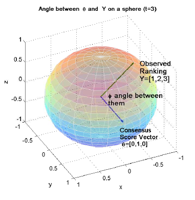
where $\kappa=\lambda\frac{t(t^{2}-1)}{12}$, and $\boldsymbol{y}$ and $\boldsymbol{\theta}$ are the standardized rankings of $\boldsymbol{R}$ and $\boldsymbol{\pi}_{0}$ respectively. However, the $\boldsymbol{\pi}_{0}$ in the distance-based model is a discrete permutation vector of integers $\{1,2,\ldots,t\}$ but the $\boldsymbol{\theta}$ in our model is a real-valued vector, representing a consensus view of the relative preference of the items from the individuals. Since both $\left\|\boldsymbol{\theta}\right\|=1$ and $\left\|\boldsymbol{y}\right\|=1$, the term $\boldsymbol{\theta}^{T}\boldsymbol{y}$ can be seen as $\cos\phi$ where $\phi$ is the angle between the consensus score vector $\boldsymbol{\theta}$ and the observation $\boldsymbol{y}$. Figure 1 illustrates an example of the angle between the consensus score vector $\boldsymbol{\theta}=(0,1,0)^{T}$ and the standardized observation of $\boldsymbol{R}=\left(1,2,3\right)^{T}$ on the sphere for $t=3$. The probability of observing a ranking is proportional to the cosine of the angle from the consensus score vector. The parameter $\kappa$ can be viewed as a concentration parameter. For small $\kappa$, the distribution of rankings will appear close to a uniform whereas for larger values of $\kappa$, the distribution of rankings will be more concentrated around the consensus score vector.

Figure 1: Illustration for the angle between the consensus score vector $\boldsymbol{\theta}=(0,1,0)^{T}$ and the standardized observation of $\left(1,2,3\right)^{T}$ on the sphere when $t=3.$

To compute the normalizing constant $C(\kappa,\boldsymbol{\theta})$, let $\text{\leavevmode{R}}_{t}$ be the set of all possible permutations of the integers $1,...,t$. Then

$$\left(C(\kappa,\boldsymbol{\theta})\right)^{-1}=\sum_{\boldsymbol{y}\in\text{\leavevmode{R}}_{t}}\exp\left\{\kappa\boldsymbol{\theta}^{T}\boldsymbol{y}\right\}.$$ (1)

Notice that the summation is over $t!$ elements in $\text{\leavevmode{R}}_{t}$. When $t$ is large, say greater than 15, the exact calculation of the normalizing constant is prohibitive. Using the fact that the set of $t!$ permutations lie on a sphere in $(t-1)$-space, our model resembles the continuous von Mises-Fisher distribution, abbreviated as $vMF(\boldsymbol{x}|\boldsymbol{m},\kappa)$, which is defined on a $\left(p-1\right)$ unit sphere with mean direction $\boldsymbol{m}$ and concentration parameter $\kappa$:

$$p(\boldsymbol{x}|\kappa,\boldsymbol{m})=V_{p}(\kappa)\exp(\kappa\boldsymbol{m}^{T}\boldsymbol{x}),$$

where

$$V_{p}(\kappa)=\frac{\kappa^{\frac{p}{2}-1}}{\left(2\pi\right)^{\frac{p}{2}}I_{\frac{p}{2}-1}(\kappa)},$$

and $I_{\frac{p}{2}-1}(\kappa)$ is the modified Bessel function of the first kind with order $\frac{p}{2}-1.$ Consequently, we may approximate the sum in (1) by an integral over the sphere. It is shown in Appendix A that

$$C(\kappa,\boldsymbol{\theta})\simeq C_{t}(\kappa)=\frac{\kappa^{\frac{t-3}{2}}}{2^{\frac{t-3}{2}}t!I_{\frac{t-3}{2}}(\kappa)\Gamma(\frac{t-1}{2})},$$

where $\Gamma(\cdot)$ is the gamma function. Table 1 shows the error rate of the approximate log-normalizing constant as compared to the exact one computed by direct summation. Here, $\kappa$ is chosen to be 0.01 to 2 and $t$ ranges from 3 to 11. Note that the exact calculation of the normalizing constant for $t=11$ requires the summation of $11!\approx 3.9\times 10^{7}$ permutations. The computer ran out of memory (16GB) beyond $t=11$. This approximation seems to be very accurate even when $t=3$. The error drops rapidly as $t$ increases. Note that this approximation allows us to approximate the first and second derivatives of $\log C$ which can facilitate our computation in what follows.

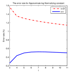
Notice that $\kappa$ may grow with $t$ as $\boldsymbol{\theta}^{T}\boldsymbol{y}$ is a sum of $t$ terms. It can be seen from the applications in Section 6 that in one of the clusters for the APA data ($t=5$), $\kappa$ is $7.44$($\approx 1.5t$) (see Table 4) while in the gene data ($t=96$), $\kappa$ is $194.34(\approx 2.0t)$ (see Table 5). We thus compute the error rate for $\kappa=t$ and $\kappa=2t$ as shown in Figure 2. It is found that the approximation is still accurate with error rate of less than 0.5% for $\kappa=t$ and is acceptable for large $t$ when $\kappa=2t$ as the error rate decreases in $t$. The von Mises-Fisher distribution was used to model compositional data by Hornik and Grün, (2014) who also provide different approaches for estimating $\kappa$ efficiently.

	$t$
$\kappa$	3	4	5	6	7	8	9	10	11
$0.01$	<0.00001%	<0.00001%	<0.00001%	<0.00001%	<0.00001%	<0.00001%	<0.00001%	<0.00001%	<0.00001%
$0.1$	<0.00001%	<0.00001%	<0.00001%	<0.00001%	<0.00001%	<0.00001%	<0.00001%	<0.00001%	<0.00001%
$0.5$	0.00003%	0.00042%	0.00024%	0.00013%	0.00007%	0.00004%	0.00003%	0.00002%	0.00001%
$0.8$	0.00051%	0.00261%	0.00150%	0.00081%	0.00046%	0.00027%	0.00017%	0.00011%	0.00008%
$1$	0.00175%	0.00607%	0.00354%	0.00194%	0.00110%	0.00066%	0.00041%	0.00027%	0.00018%
$2$	0.05361%	0.06803%	0.04307%	0.02528%	0.01508%	0.00932%	0.00598%	0.00398%	0.00273%

Table 1: The error rate of the approximate log-normalizing constant as compared to the exact one computed by direct summation.

Figure 2: The error rate of the approximate log-normalizing constant as compared to the exact one computed by direct summation for $\kappa=t$ and $\kappa=2t$.

2.2 Maximum likelihood estimation (MLE) of our model

Let $\boldsymbol{Y}=\left\{\boldsymbol{y}_{1},\ldots,\boldsymbol{y}_{N}\right\}$ be a random sample of $N$ standardized rankings drawn from $p(\boldsymbol{y}|\kappa,\boldsymbol{\theta})$. The log-likelihood of $\left(\kappa,\boldsymbol{\theta}\right)$ is then given by

$$L(\boldsymbol{Y}|\kappa,\boldsymbol{\theta})=N\ln C_{t}(\kappa)+\sum_{i=1}^{N}\kappa\boldsymbol{\theta}^{T}\boldsymbol{y}_{i}.$$ (2)

Maximizing (2) subject to $\left\|\boldsymbol{\theta}\right\|=1$ and $\kappa\geq 0$, we find that the maximum likelihood estimator of $\boldsymbol{\theta}$ is given by $\hat{\boldsymbol{\theta}}_{MLE}=\frac{\sum_{i=1}^{N}\boldsymbol{y}_{i}}{\left\|\sum_{i=1}^{N}\boldsymbol{y}_{i}\right\|},$ and $\hat{\kappa}$ is the solution of

$$A_{t}(\kappa)\equiv\frac{-C_{t}^{{}^{\prime}}(\kappa)}{C_{t}(\kappa)}=\frac{I_{\frac{t-1}{2}}\left(\kappa\right)}{I_{\frac{t-3}{2}}\left(\kappa\right)}=\frac{\left\|\sum_{i=1}^{N}\boldsymbol{y}_{i}\right\|}{N}\equiv r.$$ (3)

A simple approximation to the solution of (3) following Banerjee et al., (2005) is given by

$$\hat{\kappa}_{MLE}=\frac{r(t-1-r^{2})}{1-r^{2}}.$$

A more precise approximation can be obtained from a few iterations of Newton’s method. Using the method suggested by Sra, (2012), starting from an initial value $\kappa_{0}$, we can recursively update $\kappa$ by iteration:

$$\kappa_{i+1}=\kappa_{i}-\frac{A_{t}(\kappa_{i})-r}{1-A_{t}(\kappa_{i})^{2}-\frac{t-2}{\kappa_{i}}A_{t}(\kappa_{i})},\;i=0,1,2,\ldots.$$

2.3 Bayesian method with conjugate prior and posterior

Taking a Bayesian approach, we consider the following conjugate prior for $(\kappa,\boldsymbol{\theta})$ as

$$p(\kappa,\boldsymbol{\theta})\propto\left[C_{t}(\kappa)\right]^{\nu_{0}}\exp\left\{\beta_{0}\kappa\boldsymbol{m}_{0}^{T}\boldsymbol{\theta}\right\},$$ (4)

where $\left\|\boldsymbol{m}_{0}\right\|=1$, $\nu_{0},\beta_{0}\geq 0$. Given $\boldsymbol{Y}$, the posterior density of $(\kappa,\boldsymbol{\theta})$ can be expressed by

$$p(\kappa,\boldsymbol{\theta}|\boldsymbol{Y})\propto\exp\left\{\beta\kappa\boldsymbol{m}^{T}\boldsymbol{\theta}\right\}V_{t}(\beta\kappa)\frac{\left[C_{t}(\kappa)\right]^{N+\nu_{0}}}{V_{t}(\beta\kappa)},$$

where $\boldsymbol{m}=\left(\beta_{0}\boldsymbol{m}_{\boldsymbol{0}}+\sum_{i=1}^{N}\boldsymbol{y}_{i}\right)\beta^{-1},$ $\beta=\left\|\beta_{0}\boldsymbol{m}_{0}+\sum_{i=1}^{N}\boldsymbol{y}_{i}\right\|$. The posterior density can be factorized as

$$p(\kappa,\boldsymbol{\theta}|\boldsymbol{Y})=p(\boldsymbol{\theta}|\kappa,\boldsymbol{Y})p(\kappa|\boldsymbol{Y}),$$ (5)

where $p(\boldsymbol{\theta}|\kappa,\boldsymbol{Y})\sim vMF(\boldsymbol{\theta}|\boldsymbol{m},\beta\kappa)$ and

$$p(\kappa|\boldsymbol{Y})\propto\frac{\left[C_{t}(\kappa)\right]^{N+\nu_{0}}}{V_{t}(\beta\kappa)}=\frac{\kappa^{\frac{t-3}{2}(\upsilon_{0}+N)}I_{\frac{t-2}{2}}(\beta\kappa)}{\left[I_{\frac{t-3}{2}}(\kappa)\right]^{\nu_{0}+N}\left(\beta\kappa\right)^{\frac{t-2}{2}}}.$$

The normalizing constant for $p(\kappa|\boldsymbol{Y})$ is not available in closed form. Nunez-Antonio and Gutiérrez-Pena, (2005) suggested using a sampling-importance-resampling (SIR) procedure with a proposal density chosen to be the gamma density with mean $\hat{\kappa}_{MLE}$ and variance equal to some pre-specified number such as 50 or 100. However, in a simulation study, it was found that the choice of this variance is crucially related to the performance of SIR. An improper choice of variance may lead to slow or unsuccessful convergence. Also the MCMC method leads to intensive computational complexity. Furthermore, when the sample size $N$ is large, $\beta\kappa$ can be very large which complicates the computation of the term $I_{\frac{t-2}{2}}\left(\left(\beta\kappa\right)\right)$ in $V_{t}(\beta\kappa).$ Thus the calculation of the weights in the SIR method will fail when $N$ is large. We conclude that in view of the difficulties for directly sampling from $p(\kappa|\boldsymbol{Y})$, it may be preferable to approximate the posterior distribution with an alternative method known as variational inference (abbreviated VI from here on).

3 Variational Inference

VI provides a deterministic approximation to an intractable posterior density through optimization. It has been used in many applications and tends to be faster than classical methods, such as Markov Chain Monte Carlo (MCMC) sampling and is easier to scale to large data. The basic idea behind VI is to first posit a candidate family of densities and then to select the member of that family which is closest to the target posterior density as measured by the Kullback-Leibler divergence. If $q\left(\boldsymbol{Z}\right)$ represents the candidate family and $p\left(\boldsymbol{Z}|\boldsymbol{Y}\right)$ represents the target posterior density, the Kullback-Leibler divergence is given by

$$KL\left(q|p\right)=E_{q}\left[\ln\frac{q\left(\boldsymbol{Z}\right)}{p\left(Z|\boldsymbol{Y}\right)}\right].$$

See Blei et al., (2017) for a more comprehensive discussion of VI. We first adopt a joint vMF-Gamma distribution as the prior for $(\kappa,\boldsymbol{\theta})$:

$$p(\kappa,\boldsymbol{\theta}) =p(\boldsymbol{\theta}|\kappa)p(\kappa)$$

$$=vMF(\boldsymbol{\theta}|\boldsymbol{m}_{0},\beta_{0}\kappa)Gamma(\kappa|a_{0},b_{0}),$$

where $Gamma(\kappa|a_{0},b_{0})$ is the Gamma density function with shape parameter $a_{0}$ and rate parameter $b_{0}$ (i.e., mean equal to $\frac{a_{0}}{b_{0}}$), and $p(\boldsymbol{\theta}|\kappa)=vMF(\boldsymbol{\theta}|\boldsymbol{m}_{0},\beta_{0}\kappa)$. The choice of $Gamma(\kappa|a_{0},b_{0})$ for $p(\kappa)$ is motivated by the fact that for large values of $\kappa$, $p(\kappa)$ based on (5) tends to take the shape of a Gamma density. In fact, for large values of $\kappa$, $I_{\frac{t-3}{2}}(\kappa)\simeq\frac{e^{\kappa}}{\sqrt{2\pi\kappa}},$ and hence $p(\kappa)$ becomes the Gamma density with shape $(\nu_{0}-1)\frac{t-2}{2}+1$ and rate $\nu_{0}-\beta_{0}$:

$$p(\kappa)\propto\frac{\left[C_{t}(\kappa)\right]^{\nu_{0}}}{V_{t}(\kappa\beta)}\simeq\kappa^{(\nu_{0}-1)\frac{t-2}{2}}\exp(-(\nu-\beta)\kappa).$$

In a similar vein, Forbes and Mardia, (2015) used a similar Gamma-based approximation to develop an algorithm for sampling from the Bessel exponential posterior distribution for $\kappa.$

Under the usual variational Bayesian methods, all variables are assumed to be mutually independent. This is known as the mean-field approximation. However, inspired by the conjugate posterior distribution (5), we adopt a structural factorization of the variational posterior as $q(\boldsymbol{\theta},\kappa)=q(\boldsymbol{\theta}|\kappa)q(\kappa)$ which retains the dependency between $\boldsymbol{\theta}$ and $\kappa$.

3.1 Optimization of the variational distribution

In the variational inference framework, we aim to determine $q$ so as to minimize the Kullback-Leibler (KL) divergence between $p(\boldsymbol{\theta},\kappa|\boldsymbol{Y})$ and $q(\boldsymbol{\theta},\kappa)$. This can be shown to be equivalent to maximizing the evidence lower bound (ELBO) (Blei et al.,, 2017). So the optimization of the variational factors $q(\boldsymbol{\theta}|\kappa)$ and $q(\kappa)$ is performed by maximizing the evidence lower bound $\mathcal{L}(q)$ with respect to $q$ on the log-marginal likelihood, which in our model is given by

$$\mathcal{L}(q) =E_{q(\boldsymbol{\theta},\kappa)}\left[\ln\frac{p(\boldsymbol{y}|\kappa,\boldsymbol{\theta})p(\boldsymbol{\theta}|\kappa)p(\kappa)}{q(\boldsymbol{\theta}|\kappa)q(\kappa)}\right]$$ (6)

$$=E_{q(\boldsymbol{\theta},\kappa)}\left[f(\boldsymbol{\theta},\kappa)\right]-E_{q(\boldsymbol{\theta},\kappa)}\left[\ln q(\boldsymbol{\theta}|\kappa)\right]-E_{q(\kappa)}\left[\ln q(\kappa)\right]+constant,$$

where all the expectations are taken with respect to $q(\boldsymbol{\theta},\kappa)$ and

$$f(\boldsymbol{\theta},\kappa) =\sum_{i=1}^{N}\kappa\boldsymbol{\theta}^{T}\boldsymbol{y}_{i}+N\left(\frac{t-3}{2}\right)\ln\kappa-N\ln I_{\frac{t-3}{2}}(\kappa)+\kappa\beta_{0}\boldsymbol{m}_{0}^{T}\boldsymbol{\theta}$$

$$+\left(\frac{t-2}{2}\right)\ln\kappa-\ln I_{\frac{t-2}{2}}(\kappa\beta_{0})+(a_{0}-1)\ln\kappa-b_{0}\kappa.$$

For fixed $\kappa$, the optimal posterior distribution $\ln q^{*}(\boldsymbol{\theta}|\kappa)$ is $\ln q^{*}(\boldsymbol{\theta}|\kappa)=\kappa\beta_{0}\boldsymbol{m}_{0}^{T}\boldsymbol{\theta}+\sum_{i=1}^{N}\kappa\boldsymbol{\theta}^{T}\boldsymbol{y}_{i}+constant.$ We recognize $q^{*}(\boldsymbol{\theta}|\kappa)$ as a von Mises-Fisher distribution $vMF(\boldsymbol{\theta}|\boldsymbol{m},\kappa\beta)$ where

$$\beta=\left\|\beta_{0}\boldsymbol{m}_{0}+\sum_{i=1}^{N}\boldsymbol{y}_{i}\right\|\;\text{ and }\;\boldsymbol{m}=\left(\beta_{0}\boldsymbol{m}_{0}+\sum_{i=1}^{N}\boldsymbol{y}_{i}\right)\beta^{-1}.$$

Let $g(\kappa)$ denote the remaining terms in $f(\boldsymbol{\theta},\kappa)$ which only involve $\kappa$:

$$g(\kappa) =\left[N\left(\frac{t-3}{2}\right)+a_{0}-1\right]\ln\kappa-b_{0}\kappa-N\ln I_{\frac{t-3}{2}}(\kappa)-\ln I_{\frac{t-2}{2}}(\kappa\beta_{0})+\ln I_{\frac{t-2}{2}}(\kappa\beta).$$

It is still difficult to maximize $E_{q(\kappa)}\left[g(\kappa)\right]-E_{q(\kappa)}\left[\ln q(\kappa)\right]$ since it involves the evaluation of the expected modified Bessel function. Follow the similar idea in Taghia et al., (2014), we first find a tight lower bound $\underline{g(\kappa)}$ for $g(\kappa)$ so that

$$\mathcal{L}(q)\geq\underline{\mathcal{L}(q)}=E_{q(\kappa)}\left[\underline{g(\kappa)}\right]-E_{q(\kappa)}\left[\ln q(\kappa)\right]+constant.$$

From the properties of the modified Bessel function of the first kind, it is known that the function $\ln I_{\nu}(x)$ is strictly concave with respect to $x$ and strictly convex relative to $\ln x$ for all $\nu>0$. Then, we can have the following two inequalities:

$$\ln I_{\nu}(x)\leq\ln I_{\nu}(\bar{x})+\left(\frac{\partial}{\partial x}\ln I_{\nu}(\bar{x})\right)(x-\bar{x}),$$ (7)

$$\ln I_{\nu}(x)\geq\ln I_{\nu}(\bar{x})+\left(\frac{\partial}{\partial x}\ln I_{\nu}(\bar{x})\right)\bar{x}(\ln x-\ln\bar{x}).$$ (8)

where $\frac{\partial}{\partial x}\ln I_{\nu}(\bar{x})$ is the first derivative of $\ln I_{\nu}(x)$ evaluated at $x=\bar{x}$. Applying inequality (7) for $\ln I_{\frac{t-3}{2}}(\kappa)$ and inequality (8) for $\ln I_{\frac{t-2}{2}}(\kappa\beta_{0})$, we have

$$g(\kappa) \geq\underline{g(\kappa)}=\left[N\left(\frac{t-3}{2}\right)+a_{0}-1\right]\ln\kappa-b_{0}\kappa+\ln I_{\frac{t-2}{2}}(\beta\bar{\kappa})$$

$$+\frac{\partial}{\partial\beta\kappa}\ln I_{\frac{t-2}{2}}(\beta\bar{\kappa})\beta\bar{\kappa}\left(\ln\beta\kappa-\ln\beta\bar{\kappa}\right)-N\ln I_{\frac{t-3}{2}}(\bar{\kappa})$$

$$-N\frac{\partial}{\partial\kappa}\ln I_{\frac{t-3}{2}}(\bar{\kappa})\left(\kappa-\bar{\kappa}\right)-N\ln I_{\frac{t-2}{2}}(\beta_{0}\bar{\kappa})-N\frac{\partial}{\partial\beta_{0}\kappa}\ln I_{\frac{t-2}{2}}(\beta_{0}\bar{\kappa})\beta_{0}\left(\kappa-\bar{\kappa}\right).$$

Since the equality holds when $\kappa=\bar{\kappa}$, we see that the lower bound of $\mathcal{L}(q)$ is tight. Rearranging the terms, we have the approximate optimal solution as $\ln q^{*}(\kappa)=(a-1)\ln\kappa-b\kappa+constant,$ where

$$a=a_{0}+N\left(\frac{t-3}{2}\right)+\beta\bar{\kappa}\left[\frac{\partial}{\partial\beta\kappa}\ln I_{\frac{t-2}{2}}(\beta\bar{\kappa})\right],$$ (9)

$$b=b_{0}+N\frac{\partial}{\partial\kappa}I_{\frac{t-3}{2}}(\bar{\kappa})+\beta_{0}\left[\frac{\partial}{\partial\beta_{0}\kappa}\ln I_{\frac{t-2}{2}}(\beta_{0}\bar{\kappa})\right].$$ (10)

We also recognize $q^{*}(\kappa)$ to be a $Gamma(\kappa|a,b)$ with shape $a$ and rate $b$. The posterior mode $\bar{\kappa}$ obtained from the previous iteration as:

$$\bar{\kappa}=\begin{cases}\frac{a-1}{b}&\mbox{if }a>1,\\ \frac{a}{b}&\mbox{otherwise.}\end{cases}$$ (11)

A summary of the algorithm for our estimation is shown in Algorithm 1.

Input: Scaled $\boldsymbol{Y}=\left\{\boldsymbol{y}_{1},...,\boldsymbol{y}_{N}\right\}$

Step 1: Initialization

1. Set the prior parameters: $\beta_{0}$, $\boldsymbol{m}_{0}$, $a_{0}$ and $b_{0}$.

2. Calculate the posterior parameters for $q^{*}(\boldsymbol{\theta}|\kappa)$: $\boldsymbol{m}$, $\beta$.

3. Calculate the initial value of $\bar{\kappa}=\frac{a_{0}}{b_{0}}$.

Step 2: Optimization of the posterior distribution

repeat

1. Update posterior parameter $a$ and $b$ by (9) and (10) respectively.

2. Update $\bar{\kappa}$ by (11).

until convergence

Algorithm 1 Bayesian Estimation using variational inference of our model

3.2 Predictive density of our model

We may derive the predictive density for a new standardized ranking $\tilde{\boldsymbol{y}}$ given the observed data $\boldsymbol{Y}$. The exact predictive density is given by

$$p(\tilde{\boldsymbol{y}}|\boldsymbol{Y})=\int\int p(\tilde{\boldsymbol{y}}|\kappa,\boldsymbol{\theta})p(\kappa,\boldsymbol{\theta}|\boldsymbol{Y})\,d\kappa d\boldsymbol{\theta}.$$ (12)

We can approximate this density by first replacing the true posterior distribution with its variational approximation as:

$$p(\tilde{\boldsymbol{y}}|\boldsymbol{Y}) \approx q(\tilde{\boldsymbol{y}}|\boldsymbol{Y})=\int\int p(\tilde{\boldsymbol{y}}|\kappa,\boldsymbol{\theta})q(\boldsymbol{\theta}|\kappa,\boldsymbol{Y})q(\kappa|\boldsymbol{Y})\,d\kappa d\boldsymbol{\theta}$$

$$=\int\int p(\tilde{\boldsymbol{y}}|\kappa,\boldsymbol{\theta})vMF(\boldsymbol{\theta}|\boldsymbol{m},\beta\kappa)d\boldsymbol{\theta}Gamma(\kappa|a,b)\,d\kappa$$ (13)

where $\kappa$, $\beta$, $a$ and $b$ are the posterior parameters calculated from our algorithm.

After using a second-order approximation of the Bessel function, the approximate predictive density of $\tilde{\boldsymbol{y}}$ can be obtained by:

$$q(\tilde{\boldsymbol{y}}|\boldsymbol{Y})\approx h(\tilde{\boldsymbol{y}})l(\bar{\kappa})e^{r(\tilde{\boldsymbol{y}})\bar{\kappa}}\bar{\kappa}^{-s(\tilde{\boldsymbol{y}})}\frac{b^{a+\frac{t-1}{2}-1}\Gamma(a+s(\tilde{\boldsymbol{y}})+\frac{t-1}{2}-1)}{\left(b+r(\tilde{\boldsymbol{y}})\right)^{a+s(\tilde{\boldsymbol{y}})+\frac{t-1}{2}-1}\Gamma(a+\frac{t-1}{2}-1)},$$

where $\eta(\tilde{\boldsymbol{y}})=\left\|\tilde{\boldsymbol{y}}+\beta\boldsymbol{m}\right\|$ and

$$s(\tilde{\boldsymbol{y}})=-\eta^{2}(\tilde{\boldsymbol{y}})\bar{\kappa}^{2}\left(\frac{I^{\prime}_{\frac{t-2}{2}}(\eta(\tilde{\boldsymbol{y}})\bar{\kappa})}{I_{\frac{t-2}{2}}(\eta(\tilde{\boldsymbol{y}})\bar{\kappa})}\right)^{\prime}+\beta^{2}\bar{\kappa}^{2}\left(\frac{I^{\prime}_{\frac{t-2}{2}}(\beta\bar{\kappa})}{I_{\frac{t-2}{2}}(\beta\bar{\kappa})}\right)^{\prime}+\bar{\kappa}^{2}\left(\frac{I^{\prime}_{\frac{t-3}{2}}(\bar{\kappa})}{I_{\frac{t-3}{2}}(\bar{\kappa})}\right)^{\prime},$$

$$r(\tilde{\boldsymbol{y}})=\frac{s(\tilde{\boldsymbol{y}})}{\bar{\kappa}}-\eta(\tilde{\boldsymbol{y}})\frac{I^{\prime}_{\frac{t-2}{2}}(\eta(\tilde{\boldsymbol{y}})\bar{\kappa})}{I_{\frac{t-2}{2}}(\eta(\tilde{\boldsymbol{y}})\bar{\kappa})}+\beta\frac{I^{\prime}_{\frac{t-2}{2}}(\beta\bar{\kappa})}{I_{\frac{t-2}{2}}(\beta\bar{\kappa})}+\frac{I^{\prime}_{\frac{t-3}{2}}(\bar{\kappa})}{I_{\frac{t-3}{2}}(\bar{\kappa})},$$

$$h(\tilde{\boldsymbol{y}})=\frac{1}{\Gamma\left(\frac{t-1}{2}\right)t!2^{\frac{t-3}{2}}}\left(\frac{\beta}{\eta(\tilde{\boldsymbol{y}})}\right)^{\frac{t-2}{2}},$$

$$l(\bar{\kappa})=\frac{I_{\frac{t-2}{2}}(\eta(\tilde{\boldsymbol{y}})\bar{\kappa})}{I_{\frac{t-3}{2}}(\bar{\kappa})I_{\frac{t-2}{2}}(\beta\bar{\kappa})}.$$

The detailed derivation of the predictive density of our model can be found in Appendix B.

4 Model Extensions

4.1 Incomplete rankings

A judge may rank a set of items in accordance with some criteria. However, in real life, some of the ranking data may be missing either at random or by design. For example, in the former case, some of the items may not be ranked due to the limited knowledge of the judges. In this kind of incomplete ranking data, a missing item could have any rank and this is called subset rankings. In another instance called top-$k$ rankings, the judges may only rank the top 10 best movies among several recommended. The unranked movies would in principle receive ranks larger than $10$. In those cases, the notation $\boldsymbol{R}^{I}=(2,-,3,4,1)^{T}$ refers to a subset ranking with item 2 unranked while $\boldsymbol{R}^{I}=(2,*,*,*,1)^{T}$ represents a top two ranking with item 5 ranked first and item 1 ranked second.

In the usual Bayesian framework, missing data problems can be resolved by appealing to Gibbs sampling and data augmentation methods. Let $\left\{\boldsymbol{R}_{1}^{I},...,\boldsymbol{R}_{N}^{I}\right\}$ be a set of $N$ observed incomplete rankings, and let $\left\{\boldsymbol{R}_{1}^{*},...,\boldsymbol{R}_{N}^{*}\right\}$ be their unobserved complete rankings. We want to have the following posterior distribution:

$$p(\boldsymbol{\theta},\kappa|\boldsymbol{R}_{1}^{I},...,\boldsymbol{R}_{N}^{I})\propto p(\boldsymbol{\theta},\kappa)p(\boldsymbol{R}_{1}^{I},...,\boldsymbol{R}_{N}^{I}|\boldsymbol{\theta},\kappa),$$

which can be achieved by Gibbs sampling based on the following two full conditional distributions:

$$p(\boldsymbol{R}_{1}^{*},...,\boldsymbol{R}_{N}^{*}|\boldsymbol{R}_{1}^{I},...,\boldsymbol{R}_{N}^{I},\boldsymbol{\theta},\kappa)=\prod_{i=1}^{N}p(\boldsymbol{R}_{i}^{*}|\boldsymbol{R}_{i}^{I},\boldsymbol{\theta},\kappa),$$

$$p(\boldsymbol{\theta},\kappa|\boldsymbol{R}_{1}^{*},...,\boldsymbol{R}_{N}^{*})\propto p(\boldsymbol{\theta},\kappa)\prod_{i=1}^{N}p(\boldsymbol{R}_{i}^{*}|\boldsymbol{\theta},\kappa).$$

Sampling from $p(\boldsymbol{R}_{1}^{*},...,\boldsymbol{R}_{N}^{*}|\boldsymbol{R}_{1}^{I},...,\boldsymbol{R}_{N}^{I},\boldsymbol{\theta},\kappa)$ can be generated by using the Bayesian SIR method or the Bayesian VI method which have been discussed in the previous sections. More concretely, we need to fill in the missing ranks for each observation and for that we appeal to the concept of compatibility described in Alvo and Yu, (2014) which considers for an incomplete ranking, the class of complete order preserving rankings. For example, suppose we observe one incomplete subset ranking $\boldsymbol{R}^{I}=(2,-,3,4,1)$. The set of corresponding compatible rankings is $\left\{\left(2,5,3,4,1\right)^{T},\left(2,4,3,5,1\right)^{T},\left(2,3,4,5,1\right)^{T},\left(3,2,4,5,1\right)^{T},\left(3,1,4,5,2\right)^{T}\right\}$.

Generally speaking, let $\Omega(\boldsymbol{R}_{i}^{I})$ be the set of complete rankings compatible with $\boldsymbol{R}_{i}^{I}$. For an incomplete subset ranking with $k$ out of $t$ items being ranked, we will have a total $t!/k!$ complete rankings in its compatible set. Note that $p(\boldsymbol{R}_{i}^{*}|\boldsymbol{R}_{i}^{I},\boldsymbol{\theta},\kappa)\propto p(\boldsymbol{R}_{i}^{*}|\boldsymbol{\theta},\kappa),\>\boldsymbol{R}_{i}^{*}\in\Omega(\boldsymbol{R}_{i}^{I}).$ Obviously, direct sampling from this distribution will be tedious for large $t$. Instead, in this paper, we use the Metropolis-Hastings algorithm to draw samples from this distribution with the proposed candidates generated uniformly from $\Omega(\boldsymbol{R}_{i}^{I})$. The idea of introducing compatible rankings allows us to treat different kinds of incomplete rankings easily. It is easy to sample uniformly from the compatible rankings since we just need to fill-in the missing ranks under different situations. In the case of top-$k$ rankings, the compatibility set will be defined to ensure that the unranked items receive rankings larger than $k$. Note that it is also possible to use Monte Carlo EM approach to handle incomplete rankings under a maximum likelihood setting where the Gibbs sampling is used in the E-step (see Yu et al., (2005)).

4.2 Mixture ranking model

It is quite natural to extend our simple model to that of a mixture model in order to take into account several clusters that may exist among heterogeneous data (Lee and Yu,, 2012; Kidwell et al.,, 2008). If a population contains $G$ sub-populations (clusters), the probability of observing a standardized ranking $\boldsymbol{y}$ under our mixture model is given by

$$p(\boldsymbol{y}|\boldsymbol{\kappa},\boldsymbol{\Theta},\boldsymbol{\tau})=\sum_{g=1}^{G}\tau_{g}C_{t}(\kappa_{g})\exp\left\{\kappa_{g}\boldsymbol{\theta}_{g}^{T}\boldsymbol{y}\right\},$$

where $\boldsymbol{\tau}=(\tau_{1},\ldots,\tau_{G})$, with $\tau_{g}$ representing the proportion or the mixture weights for the $g$th sub-population whereas $\boldsymbol{\Theta}=\left(\boldsymbol{\theta}_{1},\ldots,\boldsymbol{\theta}_{G}\right)$ and $\boldsymbol{\kappa}=\left(\kappa_{1},\ldots,\kappa_{G}\right)$, with $\boldsymbol{\theta}_{g}$ and $\kappa_{g}$ are the directional and concentration parameters in the $g$th sub-population respectively. To obtain the MLE of this mixture model, we may extend the approach described in Section 2.2 using the traditional EM algorithm.

The variational inference approach for this mixture model follows the method of Taghia et al., (2014). Given a random sample of $N$ complete standardized rankings $\boldsymbol{Y}=\left\{\boldsymbol{y}_{1},\ldots,\boldsymbol{y}_{N}\right\}$ drawn from $p(\boldsymbol{y}|\boldsymbol{\kappa},\boldsymbol{\Theta},\boldsymbol{\tau})$. We first introduce a set of binary latent variables $\boldsymbol{Z}=\left\{z_{ig}\right\}$ where $i=1,\ldots,N$, $g=1,\ldots,,G$ where $z_{ig}=1$ indicates the observed ranking $\boldsymbol{y}_{i}$ belongs to the $g$th sub-population. Thus the generative model may be written as

$$p(\boldsymbol{Y},\boldsymbol{Z},\boldsymbol{\tau},\boldsymbol{\Theta},\boldsymbol{\kappa})=p(\boldsymbol{Y}|\boldsymbol{Z},\boldsymbol{\Theta},\boldsymbol{\kappa})p(\boldsymbol{\Theta},\boldsymbol{\kappa})p(\boldsymbol{Z}|\boldsymbol{\tau})p(\boldsymbol{\tau}),$$

where

$$p(\boldsymbol{Y}|\boldsymbol{Z},\boldsymbol{\Theta},\boldsymbol{\kappa}) = \prod_{i=1}^{N}\prod_{g=1}^{G}\left(C_{t}(\kappa_{g})\exp\left\{\kappa_{g}\boldsymbol{\theta}_{g}^{T}\boldsymbol{y}_{i}\right\}\right)^{z_{ig}}$$

$$p(\boldsymbol{Z}|\boldsymbol{\tau}) = \prod_{i=1}^{N}\prod_{g=1}^{G}\tau_{g}^{z_{ig}}$$

A Dirichlet distribution with prior vector parameters $d_{0,g}$ is considered for the prior distribution of $\boldsymbol{\tau}$ :

$$p(\boldsymbol{\tau})=\frac{\Gamma(\sum_{g=1}^{G}d_{0,g})}{\prod_{g=1}^{G}\varGamma\left(d_{0,g}\right)}\prod_{g=1}^{G}\tau_{k}^{d_{o,g}-1}.$$

The prior distribution for $\left(\boldsymbol{\Theta},\boldsymbol{\kappa}\right)$ is the conditional von Mises-Fisher distribution for $\boldsymbol{\Theta}|\boldsymbol{\kappa}$ and the marginal Gamma distribution for $\boldsymbol{\kappa}$:

$$p(\boldsymbol{\Theta},\boldsymbol{\kappa})=\prod_{g=1}^{G}vMF(\boldsymbol{\theta}|\boldsymbol{m}_{0,g},\beta_{0,g}\kappa_{g})Gamma(\kappa_{g}|a_{0,g},b_{0,g}),$$

where $\boldsymbol{m}_{0,g},\beta_{0,g},a_{0,g},b_{0,g}$ are the prior parameters of the $g$th sub-population. Using the similar technique in Section 3.1 to optimize the evidence lower bound given by

$$\mathcal{L_{M}}(q)=E_{q(\boldsymbol{Z},\boldsymbol{\Theta},\boldsymbol{\kappa},\boldsymbol{\tau})}\left[\ln\frac{p(\boldsymbol{Y}|\boldsymbol{Z},\boldsymbol{\Theta},\boldsymbol{\kappa})p(\boldsymbol{\Theta},\boldsymbol{\kappa})p(\boldsymbol{Z}|\boldsymbol{\tau})p(\boldsymbol{\tau})}{q(\boldsymbol{Z})q(\boldsymbol{\Theta}|\boldsymbol{\kappa})q(\boldsymbol{\kappa})q(\boldsymbol{\tau})}\right],$$ (14)

we can derive the optimal posterior distribution of each parameter.

It is not difficult to see that the optimal posterior distribution for $q(\boldsymbol{\tau})$ is recognized to be a Dirichlet distribution with parameter $d_{g}$:

$$d_{g}=d_{0,g}+\sum_{i=1}^{N}p_{ig},$$ (15)

where

$$p_{ig}=\frac{\exp(\rho_{ig})}{\sum_{j=1}^{G}\exp(\rho_{ij})},$$ (16)

$$\rho_{ig}=\frac{t-3}{2}E_{q(\kappa)}(\ln\kappa_{g})+E_{q(\boldsymbol{\tau})}\left(\ln\tau_{g}\right)+E_{q(\boldsymbol{\Theta},\boldsymbol{\kappa})}\left(\kappa_{g}\boldsymbol{\theta}_{g}^{T}\boldsymbol{y}_{i}\right)-\ln\left[2^{\frac{t-3}{2}}t!\Gamma\left(\frac{t-1}{2}\right)\right]$$ (17)

$$-\ln I_{\frac{t-3}{2}}\left(\bar{\kappa}_{g}\right)-\left(\frac{\partial}{\partial\kappa_{g}}\ln I_{\frac{t-3}{2}}\left(\bar{\kappa}_{g}\right)\right)\left[E_{q(\boldsymbol{\kappa})}\kappa_{g}-\bar{\kappa}_{g}\right],$$

$$\bar{\kappa}_{g}=\begin{cases}\frac{a_{g}-1}{b_{g}}&\mbox{if }a_{g}>1\\ \frac{a_{g}}{b_{g}}&\mbox{otherwise}\end{cases},$$ (18)

and the optimal posterior distribution of $q(\boldsymbol{\Theta}|\boldsymbol{\kappa})$ can be written as von Mises-Fisher distribution:

$$q^{*}(\boldsymbol{\Theta}|\boldsymbol{\kappa})=\prod_{g=1}^{G}vMF(\boldsymbol{\theta}_{g}|\boldsymbol{m}_{g},\kappa_{g}\beta_{g})$$

$$\beta_{g}=\left\|\beta_{0,g}\boldsymbol{m}_{0,g}+\sum_{i=1}^{N}p_{ig}\boldsymbol{y}_{i}\right\|,$$ (19)

$$\boldsymbol{m}_{g}=\left(\beta_{0,g}\boldsymbol{m}_{0,g}+\sum_{i=1}^{N}p_{ig}\boldsymbol{y}_{i}\right)\beta_{g}^{-1}.$$ (20)

Also, the optimal distribution of $q^{*}(\boldsymbol{\kappa})=\prod_{g=1}^{G}q^{*}(\kappa_{g})$ can be recognized as independent Gamma distributions:

$$q^{*}(\kappa_{g})=Gamma(\kappa_{g}|a_{g},b_{g}),$$

$$a_{g}=a_{0,g}+\left(\frac{t-3}{2}\right)\sum_{i=1}^{N}p_{ig}+\beta_{g}\bar{\kappa}_{g}\left[\frac{\partial}{\partial\beta_{g}\kappa_{g}}\ln I_{\frac{t-2}{2}}(\beta_{g}\bar{\kappa}_{g})\right],$$ (21)

$$b_{g}=b_{0,g}+\left(\sum_{i=1}^{N}p_{ig}\right)\frac{\partial}{\partial\kappa_{g}}\ln I_{\frac{t-3}{2}}(\bar{\kappa}_{g})+\beta_{0,g}\left[\frac{\partial}{\partial\beta_{0,g}\kappa_{g}}\ln I_{\frac{t-2}{2}}(\beta_{0,g}\bar{\kappa}_{g})\right],$$ (22)

and finally the optimal variational posterior distribution for $\boldsymbol{Z}$ is recognized as a multinomial distribution:

$$q^{*}(\boldsymbol{Z})=\prod_{i=1}^{N}\prod_{g=1}^{G}p_{ig}^{z_{ig}}.$$

The detailed derivation of the optimization of the mixture model can be found in Appendix C. A summary of the algorithm for estimation for this mixture model is shown in Algorithm 2.

Input: Scaled $\boldsymbol{Y}=\left\{\boldsymbol{y}_{1},...,\boldsymbol{y}_{n}\right\}$

Step 1: Initialization

1. Set the prior parameters: $d_{0,g}$, $\beta_{0,g}$, $\boldsymbol{m}_{0,g}$, $a_{0,g}$ , $b_{0,g}$ and number of clusters $G$.

2. Initialize $p_{ig}=\frac{1}{G}$ and the initial value of $\bar{\kappa}_{g}=\frac{a_{0,g}}{b_{0,g}}.$

Step 2: Optimization of the posterior distribution

repeat

1. Update posterior parameters $d_{g}$, $\beta_{g}$, $\boldsymbol{m}_{g}$, $a_{g}$ , $b_{g}$ by (15), (19), (20), (21) and (22).

2. Update $p_{ig}$ by (16) and (17).

3. Update $\bar{\kappa}_{g}$ by (18).

until convergence

Algorithm 2 Bayesian Estimation using variational inference of our mixture ranking model.

5 Simulation Studies

5.1 Comparison of the posterior distributions obtained by Bayesian SIR method and variational inference approach

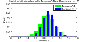
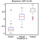
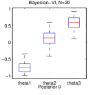
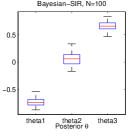
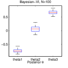
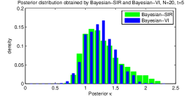
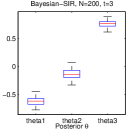
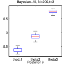
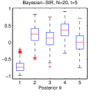
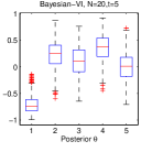
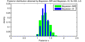
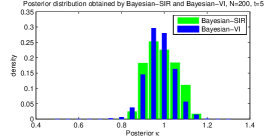
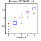
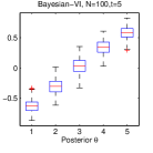
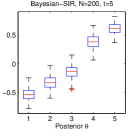
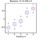
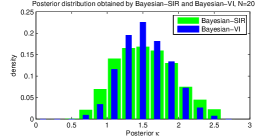
Since we use a factorized approximation for the posterior distribution in the variational inference approach, it is of interest to compare the true posterior distribution with its approximation obtained using the variational inference approach. We simulated two data sets with $\kappa=1$, $\boldsymbol{\theta}=\left(-0.71,0,0.71\right)^{T},$ $t=3$ and different data sizes of $N=20,100.$ We generated samples from the posterior distribution by SIR method in Section 2.3 using a gamma density with mean $\hat{\kappa}_{MLE}$ and variance equal to $0.2$ as the proposal density. We then applied the variational approach in Algorithm 1 and generated samples from the corresponding posterior distribution. Figure 3 exhibits the histogram and box-plot for the posterior distribution of $\kappa$ and $\boldsymbol{\theta}$.

From Figure 3, we see that the posterior distribution using the Bayesian-VI is very close to the posterior distribution obtained by the Bayesian-SIR method. When the sample size is small ($N=20$), there are more outliers for the Bayesian-SIR method while the posterior $\kappa$ for the Bayesian-VI method seems to be more concentrated. When the sample size is large, the posterior estimates of $\boldsymbol{\theta}$ and $\kappa$ become more accurate and Bayesian-VI is closer to the posterior distribution obtained by the Bayesian-SIR method. We calculate the symmetric variant of the Kullback-Leibler divergence (KLD) between two distributions obtained by two methods for posterior $\kappa$. The symmetric KLD are 0.45 for the $N=20$ case and 0.44 for the $N=100$ case. More simulations for different settings of parameters can be found in Appendix D.

Figure 3: Comparison of the posterior distribution obtained by Bayesian SIR method and the approximate posterior distribution by variational inference approach. The comparison is illustrated for different data sizes of $N=20$ (left) and $N=100$ (right).

5.2 Experiments with different sample sizes

We also evaluated the performance of the three estimating algorithms for our model when the sample size $N$ is allowed to vary from 25 to 500. We simulated three different data sets with the number of items being ranked $t=10,20,50.$ The true $\boldsymbol{\theta}$ is a random unit vector. Since our model is not a standard distribution, we use the random-walk Metropolis algorithm to draw samples from it (Liu,, 2008).

We compared the performance of the MLE method, the Bayesian method with SIR for posterior sampling (Bayesian-SIR) and the Bayesian VI. We chose non-informative priors for both Bayesian-SIR and Bayesian-VI. Specifically, the prior parameter $\boldsymbol{m}_{0}$ is chosen uniformly whereas $\beta_{0}$, $a_{0}$ and $b_{0}$ are chosen to be small numbers close to zero. For the MLE method, we perform Newton-Raphson iterations to get a more accurate $\kappa$. For the posterior distribution of $\kappa$ in the Bayesian-SIR method. we used a Gamma density with mean $\hat{\kappa}_{MLE}$ and variance 1 as the proposal density to sample $1,000$ observations of $\kappa$ from $10,000$ candidates.

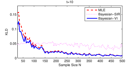
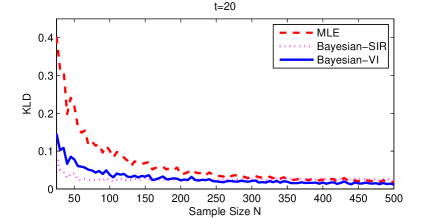
We calculated the Kullback-Leibler divergence (KLD) of the true model from the estimated model, in which the model parameters are the point estimates derived by either MLE or the posterior mean of the Bayesian method. A smaller value of KLD implies higher accuracy of the estimation method. Each experiment is repeated 10 times to smooth out the effect of random initialization and the average results are shown in Figure 4.

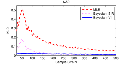
Figure 4: The KLD values between true model and its estimated model versus the Sample size $N$ for $t=10$ (top), $t=20$ (middle) and $t=50$ (bottom). The estimated model is given by the MLE method, Bayesian method with SIR for posterior sampling (Bayesian-SIR) and the Bayesian method with variational approach (Bayesian-VI). Each experiment is repeated 10 times and the average results are shown.

It can be seen from Figure 4 that large sample sizes lead to lower KLD values for the three algorithms as expected. From the comparison, when $t$ is small $(t=10)$, the Bayesian method with variational approach (Bayesian-VI) performs similar to the MLE method and works better than Bayesian-SIR. The failure of Bayesian-SIR may be the result of the variance of the proposal gamma density being too large compared to the variance of the true posterior distribution of $\kappa.$ Thus this improper choice of variance will slow down the convergence of the MCMC model. When $t$ is large ($t=20$ & $50$), Bayesian-VI and Bayesian-SIR are very close while the MLE method doesn’t work well when the sample size is small. When $N$ is large, the three approaches tend to converge to fairly similar results. Even for $t=50$ and $N=500$, the MLE method still performs slightly poorer than the Bayesian counterparts. As a whole. the Bayesian-VI generally performs the best for different sets of $t$ and $N$.

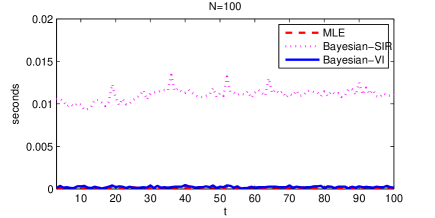
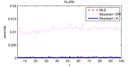
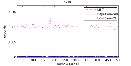
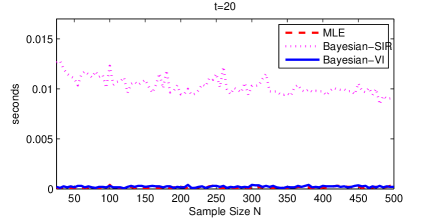
We also computed the average computation time for each set of experiments. From Figure 5, we see that the computation time for Bayesian-SIR is the slowest as expected since it is an MCMC sampling method. The speeds of Bayesian-VI and MLE are quite similar and they are about 50 to 100 times faster than Bayesian-SIR. All the simulations were conducted on a PC with 4.0 GHz quad-core CPU.

Figure 5: Average computation times (seconds) for one run versus the Sample size $N$ by the MLE method, Bayesian method with SIR (Bayesian-SIR) and the Bayesian method with variational approach (Bayesian-VI). All the simulations were conducted on a PC with 4.0 GHz quad-core CPU.

5.3 Experiments with different data dimensions

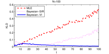
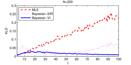
In the following experiments we compared the performances of the different approaches as the number $t$ of items ranked varies from 3 to 100. We set $\kappa=1$ and chose the true $\boldsymbol{\theta}$ to be a random unit vector. We chose $N=100,200,500$. The detailed simulation settings are the same as Section 5.2. For evaluation, we again calculated the Kullback-Leibler divergence (KLD) of the true model from the estimated model shown in Figure 6. Each experiment is repeated 10 times and the average results are shown to smooth out the effect of random initialization.

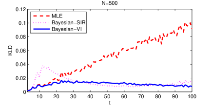
It is seen that large values of $t$ lead to the failure of the MLE method since there will be more parameters than data-points. The Bayesian-SIR method also encounters problems when $t$ is large compared to $N.$ This may be because the selected proposal density (variance $=1$) in the SIR method may be inappropriate when $t$ is large. From the comparison, the Bayesian -VI method has lower KLD values for large $t$. When $t$ is small, the MLE and Bayesian-VI have similar results while the Bayesian-SIR method has higher KLD.

We also computed the average computation time for each set of experiments. From Figure 7, the speed of convergence for Bayesian-VI and MLE are quite similar and they are about 50 to 100 times faster than Bayesian-SIR. All the simulations are conducted on a PC with 4 core 4.0 GHz CPU.

Figure 6: The KLD values between true model and its estimated model versus the data dimension $t$ (number of items being ranked) for data sizes of $N=100$ (top), $N=200$ (middle) and $N=500$ (bottom). The estimated model is given by the MLE method (MLE), Bayesian method with SIR for posterior sampling (Bayes-SIR) and the Bayesian method with variational approach (Bayes-VI). Each experiment is repeated 10 times and the average results are shown.

Figure 7: Average computation times (seconds) for one run versus the data dimension $t$ by the MLE approach (MLE), Bayesian method with SIR (Bayesian-SIR) and the Bayesian method with variational approach (Bayesian-VI). All the simulations were conducted on a PC with 4.0 GHz quad-core CPU.

5.4 Simulation for the estimation of the predictive density

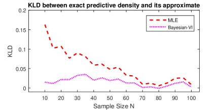
In this experiment, we compared the accuracy of the approximated predictive density between the Bayesian-VI and MLE methods. We simulated data from our model with $\kappa=1$ and $t=5$. The true $\boldsymbol{\theta}$ is a random unit vector. For each set of simulation, we considered sample sizes ranging from 10 to 100. We also calculated the Kullback-Leibler divergence (KLD) from the true posterior distribution to the approximate predictive density. The true posterior predictive distribution is calculated by Monte Carlo integration (12) numerically from the true posterior distribution obtained by the SIR method with size $10^{5}$. We calculated the approximated predictive density using the MLE method. Each experiment was repeated 10 times and the average results are shown in Figure 8.

From Figure 8, we see that the KLD for both methods decreases with increasing sample size as expected. However, for small training data, Bayesian-VI performs much better than the MLE method.

Figure 8: The KLD between the exact predictive density $p(\tilde{y}|Y)$ and the approximate predictive densities by Bayesian method with variational approach (Bayesian-VI) and MLE method (MLE). Each experiment is repeated 10 times and the average results are shown.

5.5 Simulation for incomplete rankings

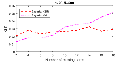
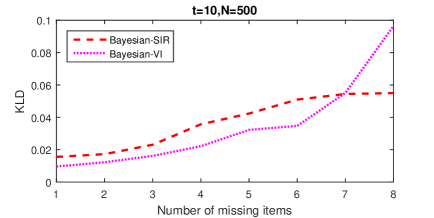
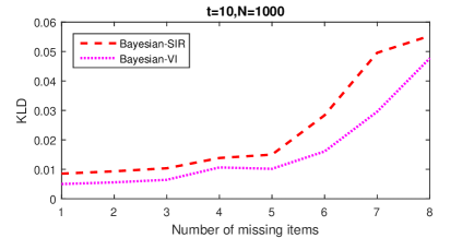
The following experiments aim to compare the performance with respect to the number of missing items $k$ when incomplete rankings are observed. We first simulated data from our model with $\kappa=1$ and $\left\|\boldsymbol{\theta}\right\|=1$. Then we randomly dropped the ranking for $k$ items and re-ranked the remaining items to get the incomplete ranking. We chose three different settings for the simulations: $\left(t=10,N=500\right)$, $\left(t=10,N=1000\right)$ and $\left(t=20,N=500\right)$. The number of missing items $k$ varies up to $\left(t-2\right)$. We also calculated the Kullback-Leibler divergence (KLD) of the true model from the estimated model to assess the impact. The estimated model is given by Gibbs samplings with the Bayesian method with SIR (Bayesian-SIR) and the Bayesian-VI in the second conditional distribution. For each iteration for the Bayesian-SIR method, we simulated $10$ samples from $100$ candidates and selected one for the next step. The result of this comparison is shown in Figure 9. Each experiment is repeated 10 times and the average results are shown to smooth out the effect of random initialization.

From Figure 9, we see that the KLD increases with increasing number of missing items as expected. From the comparison, the Bayesian-VI has lower KLD values for small number of missing items $k$ compared to the Bayesian-SIR method. This is consistent with previous simulation results. When $N$ is large ($N=1,000$), Bayesian-VI performs better than Bayesian-SIR. When the number of missing items is large, Bayesian-SIR seems to be a better choice than Bayesian-VI. However, when comparing computation time, Bayesian-VI is much faster than Bayesian-SIR.

Figure 9: The KLD values between the true model and the estimated model versus the number of missing items with different settings: $t=10$, $N=500$ (top), $t=10$, $N=1000$ (middle) and $t=20$, $N=500$ (bottom). The estimated model is given by Gibbs sampling with Bayesian method with SIR (Bayesian-SIR) and the Bayesian method with variational approach (Bayesian-VI) in the second conditional distribution. Each experiment is repeated 10 times and the average results are shown.

6 Applications

6.1 Sushi data sets

We investigate the two data sets of Kamishima, (2003) for finding the difference in food preference patterns between eastern and western Japan. Historically, western Japan has been mainly affected by the culture of the Mikado emperor and nobles, while eastern Japan has been the home of the Shogun and Samurai warriors. Therefore, the preference patterns in food are different between these two regions (Kamishima,, 2003).

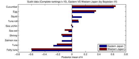
The first data set consists of complete rankings of $t=10$ different kinds of sushi given by 5000 respondents according to their preference. The region of respondents is also recorded ($N=3285$ for Eastern Japan, $1715$ for Western Japan). We apply the MLE, Bayesian-SIR and Bayesian-VI on both Eastern and Western Japan data. The settings for the priors are similar to those used in the simulations in Section 5.2. Since the sample size $N$ is quite large compared to $t$, the estimated models for all three methods are almost the same. Figure 10 compares the posterior means of $\boldsymbol{\theta}$ between Eastern Japan (Blue bar) and Western Japan (Red bar) obtained by Bayesian-VI method. Note that the more negative value of $\theta_{i}$ means that the more preferable sushi $i$ is. From Figure 10, we see that the main difference for sushi preference between Eastern and Western Japan occurs in Salmon roe, Squid, Sea eel, Shrimp and Tuna. People in Eastern Japan have a greater preference for Salmon roe and Tuna than the western Japanese. On the other hand, the latter have a greater preference for Squid, Shrimp and Sea eel. Table 2 shows the posterior parameter obtained by Bayesian-VI. It can be seen that the eastern Japanese are slightly more cohesive than western Japanese since the posterior mean of $\kappa$ is larger.

Figure 10: Posterior means of $\boldsymbol{\theta}$ for the sushi complete ranking data ($t=10$) in Eastern Japan (Blue bar) and Western Japan (Red bar) obtained by Bayesian-VI.

Posterior Parameter	Eastern Japan	Western Japan
$\beta$	1458.85	741.61
$a$	18509.84	9462.70
$b$	3801.57	2087.37
Posterior Mean of $\kappa$	4.87	4.53

Table 2: Posterior parameters for the sushi complete ranking data ($t=10$) in Eastern Japan and Western Japan obtained by Bayesian-VI.

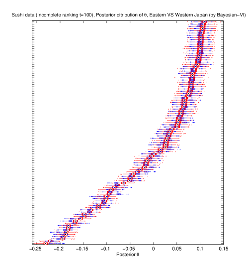
The second data set contains incomplete rankings given by 5000 respondents who were asked to pick and rank some of the $t=100$ different kinds of sushi according to their preference and most of them only selected and ranked the top 10 out of 100 sushi. Figure 11 compares the box-plots of the posterior means of $\boldsymbol{\theta}$ between Eastern Japan (Blue box) and Western Japan (Red box) obtained by Bayesian-VI. The posterior distribution of $\boldsymbol{\theta}$ is based on the Gibbs samplings after dropping the first 200 samples during the burn-in period. Since there are too many kinds of Sushi, this graph doesn’t allow us to show the name of each Sushi. However, we can see that about one third of the 100 kinds of sushi have fairly large posterior means of $\theta_{i}$ and their values are pretty close to each others. This is mainly because these sushi are less commonly preferred by Japanese and the respondents hardly chose these sushi in their list. As these sushi are usually not ranked as top 10, it is natural to see that the posterior distributions of their $\theta_{i}$’s tend to have a larger variance.

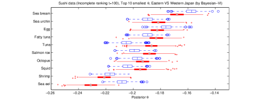
From Figure 11, we see that there exists a greater difference between eastern and western Japan for small $\theta_{i}$’s. Figure 12 compares the box-plots of the top 10 smallest posterior means of $\boldsymbol{\theta}$ between Eastern Japan (Blue box) and Western Japan (Red box). The main difference for sushi preference between Eastern and Western Japan appears to be in Sea eel, Salmon roe, Tuna, Sea urchin and Sea bream. The eastern Japanese prefer Salmon roe, Tuna and Sea urchin sushi more than the western Japanese, while the latter like Sea eel and Sea bream more than the former. Generally speaking, Tuna and Sea urchin are more oily food, while Salmon roe and Tuna are more seasonal food. So from the analysis of both data sets, we can conclude that the eastern Japanese usually prefer more oily and seasonal food than the western Japanese (Kamishima,, 2003).

Figure 11: Boxplots of the posterior means of $\boldsymbol{\theta}$ for the sushi incomplete rankings ($t=100$) in Eastern Japan (Blue box-plots) and Western Japan (Red box-plots) obtained by Bayesian-VI.

Figure 12: Box-plots of the top 10 smallest posterior means of $\boldsymbol{\theta}$ for the sushi incomplete rankings ($t=100$) in Eastern Japan (Blue box-plots and blue circles for outliers) and Western Japan (Red box-plots and red pluses for outliers) obtained by Bayesian-VI.

6.2 APA data

We revisit the well-known APA data set of Diaconis, (1988) which contains $5738$ full rankings of 5 candidates for the presidential election of the American Psychological Association (APA) in 1980. For this election, members of APA had to rank five candidates {A,B,C,D,E} in order of their preference. Candidates A and C are research psychologists, candidates D and E are clinical psychologists and candidate B is a community psychologist. This data set has been studied by Diaconis, (1988) and Kidwell et al., (2008) who found that the voting population was divided into 3 clusters.

We fit the data using the mixture model stated in Section 4.2. We chose a non-informative prior for the Bayesian-VI method for a different number of clusters $G=1$ to 5. Specifically, the prior parameter $\boldsymbol{m}_{0g}$ is a randomly chosen unit vector whereas $\beta_{0g}$, $d_{0g}$, $a_{0g}$ and $b_{0g}$ are chosen as random numbers close to zero. The $p_{ig}$ are initialized as $\frac{1}{G}$. Table 3 shows the Deviance information criterion (DIC) for $G=1$ to $5$. It can be seen that the mixture model with $G=3$ clusters attains the smallest DIC.

$G$	1	2	3	4	5
DIC	54827	53497	53281	53367	53375

Table 3: Deviance information criterion (DIC) for the APA ranking data.

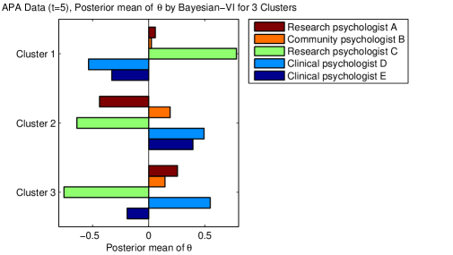
Table 4 indicates the posterior parameters for the three-cluster solution and Figure 13 exhibits the posterior means of $\boldsymbol{\theta}$ for the three clusters obtained by Bayesian-VI. It is very interesting to see that Clusters 1 vote clinical psychologists D and E as their first and second choices and dislike especially the research psychologist C. Cluster 2 prefer research psychologists A and C but dislike the others. Cluster 3 prefer research psychologist C. From Table 4, Cluster 1 represents the majority (posterior mean of $\tau_{1}=56.31\%$). Cluster 2 is small but more cohesive since the posterior mean of $\kappa_{2}$ is larger. Cluster 3 has a posterior mean of $\tau_{3}=20.73\%$ and $\kappa_{3}$ is $1.52$. The preferences of the five candidates made by the voters in the three clusters are heterogeneous and the mixture model enables us to draw further inference from the data.

Posterior Parameter	Cluster 1	Cluster 2	Cluster 3
$\boldsymbol{m}$	0.06	-0.44	0.26
	0.02	0.19	0.14
	0.78	-0.64	-0.75
	-0.54	0.49	0.55
	-0.33	0.39	-0.19
$\beta$	1067.10	1062.34	414.74
$d$	3231.09	1317.21	1189.72
$a$	4756.33	9224.97	1821.73
$b$	3330.45	1239.41	1197.80
Posterior mean of $\boldsymbol{\kappa}$	1.43	7.44	1.52
Posterior mean of $\boldsymbol{\tau}$	56.31%	22.96%	20.73%

Table 4: Posterior parameters for the APA ranking data ($t=5$) for three clusters obtained by Bayesian-VI.

Figure 13: Plot of the posterior means of $\boldsymbol{\theta}$ for the APA ranking data ($t=5$) for three clusters obtained by Bayesian-VI.

6.3 Breast cancer gene expressions data

We apply our mixture model on a ranked mRNA expression data set to classify patients into the sub-type of breast cancer. Similar topics have also been studied by Naume et al., (2007). All the raw data can be obtained from the Stanford Micro array Database (SMD) (http://genome-www5.stanford.edu/). We downloaded the mRNA expression data of 121 breast cancer patients who have two disease sub-type based on their ER/PgR-status: Estrogen Receptor negative (ER-, 41 patients) or positive (ER+, 80 patients). Our aim is to classify the breast cancer patients into two sub-groups based on their ranked gene expressions data for 96 genes ($t=96$). These 96 genes are selected from the KEGG Estrogen signaling pathway (Kyoto Encyclopedia of Genes and Genomes: hsa04915) (http://www.genome.jp/kegg/). We use the rankings of 96 normalized log 2-transformed gene expression ratios for the 121 patients as our training data.

In this experiment, we first use the patients’ gene ranking data (without knowing the true disease sub-type of each patient) to fit our mixture model ($G=2$). The prior parameter $\boldsymbol{m}_{0g}$ is a randomly chosen unit vector while the other prior parameters $\beta_{0g}$, $d_{0g}$, $a_{0g}$ and $b_{0g}$ are chosen as random small numbers close to zero. The $p_{ig}$ are initialized as $\frac{1}{G}$. Table 5 shows the posterior parameters for the gene ranking data for the two clusters obtained by Bayesian-VI. As the ER+ patients are more frequent in this data set, we label Cluster 1 as the ER+ group since the posterior mean of $\tau_{1}$ is higher (66.79%). So Cluster 2 is then labeled as the ER- group. Using our clustering solution and the true disease sub-type for the patients, Figure 14 shows the ROC (Receiver operating characteristic) curves based on the fitted two-mixture model (the left panel) and the classification implied by the K-means clustering with squared Euclidean distance (the right panel) (Hartigan and Wong,, 1979; Arthur and Vassilvitskii,, 2007). From Figure 14, it is seen that our mixture model has a greater discrimination power. The AUC (Area under the curve) for our method is 0.9183 which is higher than that for the K-means method (0.8235).

Posterior Parameter	Cluster 1 (ER+)	Cluster 2 (ER-)
$\beta$	63.68	29.75
$d$	80.84	40.18
$a$	16181.18	6462.97
$b$	83.26	42.28
Posterior mean of $\kappa$	194.34	152.85
Posterior mean of $\tau$	0.6679	0.3320

Table 5: The posterior parameter of $\theta$ for the gene ranking data ($t=96$) for two clusters using Bayesian-VI.

Figure 14: ROC curves for classifying disease sub type. The left panel is based on our fitted two-mixture model. The right panel is based on the classification implied by K-means clustering with squared Euclidean distance.

7 Conclusions and Discussion

We proposed a new class of general exponential ranking model called angle-based ranking models. The model assumed a consensus score vector $\boldsymbol{\theta}$ where the rankings reflect the rank-order preference of the items. The probability of observing a ranking is proportional to the cosine of the angle from the consensus score vector. Then we proposed a very good approximation for the normalizing constant using the von Mises-Fisher distribution which can facilitate the computation of fitting the model. Usually it is an NP-hard problem to find the estimates of parameters for other classes of ranking models when $t$ is large. However, our model avoided this problem and can easily calculate the estimate of our model. We made use of Bayesian variational inference to approximate the posterior density as well as the predictive density. This approach exhibited a great computational advantage compared to traditional MCMC methods. One can also consider to use regularization methods such as LASSO, Ridge and Elastic Net to overcome the potential over-fitting problem, especially for large $t$. In fact, regularization methods can be implemented via a Bayesian approach with suitably chosen priors. For instance, LASSO in a regression problem can be viewed as maximum a posterior method in a Bayesian framework using a Laplace prior centered at zero. It is of interest to study regularization for angle-based models and such interesting problem would be studied in the future.

Unlike distance-based models, the consensus score vector $\boldsymbol{\theta}$ proposed exhibits detailed information on item preferences while distance-based model only provide equal-spaced modal ranking. We applied the method to sushi data, and concluded that certain types of sushi are seldom eaten by the Japanese.

Model extensions to incomplete rankings and mixture models were also developed. Incomplete rankings often arise when the number of items ranked is large. The use of compatible rankings makes it possible to handle incomplete rankings such as top-$k$ rankings, and subsets ranking. The mixture models can be used as a model-based clustering tool for ranking data.

Our consensus score vector $\boldsymbol{\theta}$ defined on a unit sphere can be easily reparameterized to incorporate additional arguments or covariates in the model. the judge-specific covariates could be age, gender and income, and the item-specific covariates could be prices, weights and brands, and the judge-item-specific covariates could be some personal experience on using each phone or brand. Adding those covariates into the model will greatly improve the power of prediction of our model. We can also develop Bayesian inference methods to facilitate the computation. This interesting problem will be deferred to later papers.

Appendix A. Derivation of the approximation for normalizing constant of our model

Since $t!$ permutations lie on a sphere in $(t-1)$-space, our model is very close to another exponential family distribution, the von Mises-Fisher distribution which is defined on a unit sphere. Consider a von Mises-Fisher distribution defined on a $(t-1)$-space, its normalizing constant can be written as the integration on a unit $(t-2)$-sphere:

$$V_{t-1}(\kappa)^{-1}=\frac{(2\pi)^{\frac{t-1}{2}}I_{\frac{t-3}{2}}(\kappa)}{\kappa^{\frac{t-3}{2}}}=\int_{\left\|\boldsymbol{x}\right\|=1}\exp\left\{\kappa\boldsymbol{\theta}^{T}\boldsymbol{x}\right\}d\boldsymbol{x}.$$ (23)

Using a naive Monte Carlo integration, we have

$$\int_{\left\|\boldsymbol{x}\right\|=1}\exp\left\{\kappa\boldsymbol{\theta}^{T}\boldsymbol{x}\right\}dx\simeq S\frac{1}{n}\sum_{i=1}^{n}\exp\left\{\kappa\boldsymbol{\theta}^{T}\boldsymbol{x}_{i}\right\},$$

where $\left\{x_{i}\right\}$ are uniformly distributed on a $(t-2)$-unit sphere, and $S=\int_{\left\|\boldsymbol{x}\right\|=1}d\boldsymbol{x}$.

Summing over all possible $t!$ permutations $y_{i}$ we can further write:

$$\int_{\left\|\boldsymbol{x}\right\|=1}\exp\left\{\kappa\boldsymbol{\theta}^{T}\boldsymbol{x}\right\}d\boldsymbol{x}\simeq S\frac{1}{t!}\sum_{i=1}^{t!}\exp\left\{\kappa\boldsymbol{\theta}^{T}\boldsymbol{y}_{i}\right\}.$$ (24)

Note that

$$S=\int_{\left\|\boldsymbol{x}\right\|=1}d\boldsymbol{x}=\frac{2\pi^{\frac{t-1}{2}}}{\Gamma(\frac{t-1}{2})}$$

is actually the surface of the unit $(t-2)$-sphere. After combining (23) and (24), we can have the inverse of the approximation for normalizing constant of our model:

$$C_{t}(\kappa)^{-1}=\sum_{\boldsymbol{y}\in\text{\leavevmode{R}}_{t}}\exp\left\{\kappa\boldsymbol{\theta}^{T}\boldsymbol{y}\right\} \simeq\frac{t!}{S}V_{t-1}(\kappa)^{-1}$$

$$=\frac{t!}{S}\cdot\frac{(2\pi)^{\frac{t-1}{2}}I_{\frac{t-3}{2}}(\kappa)}{\kappa^{\frac{t-3}{2}}}$$

$$=\frac{2^{\frac{t-3}{2}}t!I_{\frac{t-3}{2}}(\kappa)\Gamma(\frac{t-1}{2})}{\kappa^{\frac{t-3}{2}}}.$$

Note that when $\kappa=0$, the $V_{t-1}(\kappa)^{-1}$ becomes the surface of a unit $(t-2)$-sphere: $V_{t-1}(\kappa)^{-1}=S$. Then the approximation for normalizing constant of our model becomes:$C_{t}(\kappa)\simeq\frac{S}{t!}S^{-1}=\frac{1}{t!}$, which is equal to the exact normalizing constant of our model for $\kappa=0$.

Appendix B. Detailed Derivation of the predictive density of our model

To obtain the predictive density of our model, we first integrate (13) over $\boldsymbol{\theta}$:

$$\int p(\tilde{\boldsymbol{y}}|\kappa,\boldsymbol{\theta})vMF(\boldsymbol{\theta}|\boldsymbol{m},\beta\kappa)d\boldsymbol{\theta} =C_{t}(\kappa)V_{t}(\beta\kappa)\int\exp\left[\kappa\boldsymbol{\theta}^{T}\tilde{\boldsymbol{y}}+\beta\kappa\boldsymbol{m}^{T}\boldsymbol{\theta}\right]d\boldsymbol{\theta}$$

$$=C_{t}(\kappa)V_{t}(\beta\kappa)V_{t}(\kappa\eta(\tilde{\boldsymbol{y}}))^{-1}\int V_{t}(\kappa\eta(\tilde{\boldsymbol{y}}))\exp\left[\kappa\eta(\tilde{\boldsymbol{y}})\frac{\tilde{\boldsymbol{y}}^{T}+\beta\boldsymbol{m}^{T}}{\eta(\tilde{\boldsymbol{y}})}\boldsymbol{\theta}\right]d\boldsymbol{\theta}$$

where $\eta(\tilde{\boldsymbol{y}})=\left\|\tilde{\boldsymbol{y}}+\beta\boldsymbol{m}\right\|$. This involves integrating a vMF with mean direction $\tilde{\boldsymbol{y}}+\beta\boldsymbol{m}$ and concentration parameter $\kappa\eta(\tilde{\boldsymbol{y}})$. Hence, we can replace the known normalizing constant for vMF as:

$$\int p(\tilde{\boldsymbol{y}}|\kappa,\boldsymbol{\theta})vMF(\boldsymbol{\theta}|\boldsymbol{m},\beta\boldsymbol{\kappa})d\boldsymbol{\theta} =C_{t}(\kappa)V_{t}(\beta\kappa)V_{t}(\kappa\eta(\tilde{\boldsymbol{y}}))^{-1}$$

$$=h(\tilde{\boldsymbol{y}})l(\kappa)\kappa^{\frac{t-3}{2}},$$ (25)

where

$$h(\tilde{\boldsymbol{y}})=\frac{1}{\Gamma\left(\frac{t-1}{2}\right)t!2^{\frac{t-3}{2}}}\left(\frac{\beta}{\eta(\tilde{\boldsymbol{y}})}\right)^{\frac{t-2}{2}},$$

$$l(\kappa)=\frac{I_{\frac{t-2}{2}}(\eta(\tilde{\boldsymbol{y}})\kappa)}{I_{\frac{t-3}{2}}(\kappa)I_{\frac{t-2}{2}}(\beta\kappa)}.$$

Substituting (25) into $q(\tilde{\boldsymbol{y}}|\boldsymbol{Y})$ in (13), we have

$$q\left(\tilde{\boldsymbol{y}}|\boldsymbol{Y}\right)=h(\tilde{\boldsymbol{y}})\frac{b^{a+\frac{t-1}{2}-1}}{\Gamma(a+\frac{t-1}{2}-1)}\int l(\kappa)e^{-b\kappa}\kappa^{a+\frac{t-1}{2}-2}d\kappa.$$ (26)

Since the term $l(\kappa)$ involves three Bessel functions, we can use a second order approximation of $\ln l(\kappa)$ in terms of $\kappa$ and $\ln\kappa$ as:

$$\ln l(\kappa)\approx\ln l(\bar{\kappa})-r(\tilde{\boldsymbol{y}})\left(\kappa-\bar{\kappa}\right)+s(\tilde{\boldsymbol{y}})(\ln\kappa-\ln\bar{\kappa}),$$ (27)

where $r(\tilde{\boldsymbol{y}})$ and $s(\tilde{\boldsymbol{y}})$ are calculated from the first and second order derivatives expanded at $\bar{\kappa}$.

This yields:

$$s(\tilde{\boldsymbol{y}})=-\eta^{2}(\tilde{\boldsymbol{y}})\bar{\kappa}^{2}\left(\frac{I^{\prime}_{\frac{t-2}{2}}(\eta(\tilde{\boldsymbol{y}})\bar{\kappa})}{I_{\frac{t-2}{2}}(\eta(\tilde{\boldsymbol{y}})\bar{\kappa})}\right)^{\prime}+\beta^{2}\bar{\kappa}^{2}\left(\frac{I^{\prime}_{\frac{t-2}{2}}(\beta\bar{\kappa})}{I_{\frac{t-2}{2}}(\beta\bar{\kappa})}\right)^{\prime}+\bar{\kappa}^{2}\left(\frac{I^{\prime}_{\frac{t-3}{2}}(\bar{\kappa})}{I_{\frac{t-3}{2}}(\bar{\kappa})}\right)^{\prime},$$

$$r(\tilde{\boldsymbol{y}})=\frac{s(\tilde{\boldsymbol{y}})}{\bar{\kappa}}-\eta(\tilde{\boldsymbol{y}})\frac{I^{\prime}_{\frac{t-2}{2}}(\eta(\tilde{\boldsymbol{y}})\bar{\kappa})}{I_{\frac{t-2}{2}}(\eta(\tilde{\boldsymbol{y}})\bar{\kappa})}+\beta\frac{I^{\prime}_{\frac{t-2}{2}}(\beta\bar{\kappa})}{I_{\frac{t-2}{2}}(\beta\bar{\kappa})}+\frac{I^{\prime}_{\frac{t-3}{2}}(\bar{\kappa})}{I_{\frac{t-3}{2}}(\bar{\kappa})}.$$

The quantities $\frac{I^{\prime}_{v}(x)}{I_{v}(x)}$ and $\left(\frac{I^{\prime}_{v}(x)}{I_{v}(x)}\right)^{\prime}$ can be computed using the recurrence relation of the derivative of the modified Bessel function of the first kind:

$$\frac{I^{\prime}_{v}(x)}{I_{v}(x)}=\frac{I_{v+1}(x)}{I_{v}(x)}+\frac{v}{x}$$

$$\left(\frac{I^{\prime}_{v}(x)}{I_{v}(x)}\right)^{\prime}=-\frac{v}{x^{2}}+1-\frac{2v+1}{x}\left(\frac{I_{v+1}(x)}{I_{v}(x)}\right)-\left(\frac{I_{v+1}(x)}{I_{v}(x)}\right)^{2}.$$

Using (27), then the integration over $\kappa$ can be approximated by

$$\int l(\kappa)e^{-b\kappa}\kappa^{a+\frac{t-1}{2}-2}d\kappa \approx l(\bar{\kappa})e^{r(\tilde{\boldsymbol{y}})\bar{\kappa}}\bar{\kappa}^{-s(\tilde{\boldsymbol{y}})}\int e^{-\kappa\left(b+r(\tilde{\boldsymbol{y}})\right)}\kappa^{a+s(\tilde{\boldsymbol{y}})+\frac{t-1}{2}-2}d\kappa$$

$$=l(\bar{\kappa})e^{r(\tilde{\boldsymbol{y}})\bar{\kappa}}\bar{\kappa}^{-s(\tilde{\boldsymbol{y}})}\Gamma\left(a+s(\tilde{\boldsymbol{y}})+\frac{t-1}{2}-1\right)\left(b+r(\tilde{\boldsymbol{y}})\right)^{-(a+s(\tilde{\boldsymbol{y}})+\frac{t-1}{2}-1)}$$ (28)

where the integration involves a Gamma distribution with shape parameter

$$a+s(\tilde{\boldsymbol{y}})+\frac{t-1}{2}-1$$

and rate parameter

$$b+r(\tilde{\boldsymbol{y}}).$$

Hence, plugging in the known normalizing constant of the Gamma distribution, we see that the approximate predictive density of $\tilde{\boldsymbol{y}}$ can be obtained by substituting (28) in (26):

$$q(\tilde{\boldsymbol{y}}|\boldsymbol{Y})\approx h(\tilde{\boldsymbol{y}})l(\bar{\kappa})e^{r(\tilde{\boldsymbol{y}})\bar{\kappa}}\bar{\kappa}^{-s(\tilde{\boldsymbol{y}})}\frac{b^{a+\frac{t-1}{2}-1}\Gamma(a+s(\tilde{\boldsymbol{y}})+\frac{t-1}{2}-1)}{\left(b+r(\tilde{\boldsymbol{y}})\right)^{a+s(\tilde{\boldsymbol{y}})+\frac{t-1}{2}-1}\Gamma(a+\frac{t-1}{2}-1)}.$$

Appendix C. Derivation of the variational inference of the mixture ranking model

For the mixture model, the evidence lower bound is given by

$$\mathcal{L_{M}}(q)=E_{q(\boldsymbol{Z},\boldsymbol{\Theta},\boldsymbol{\kappa},\boldsymbol{\tau})}\left[\ln\frac{p(\boldsymbol{R}|\boldsymbol{Z},\boldsymbol{\Theta},\kappa)p(\boldsymbol{\Theta},\kappa)p(\boldsymbol{Z}|\tau)p(\tau)}{q(\boldsymbol{Z})q(\boldsymbol{\Theta}|\boldsymbol{\kappa})q(\boldsymbol{\kappa})q(\tau)}\right].$$ (29)

Focusing first on terms involving $Z$, we have from (29)

$$\mathcal{L}(q) =E_{q(\boldsymbol{Z},\boldsymbol{\Theta},\boldsymbol{\kappa},\boldsymbol{\tau})}\left[\ln\left(p(\boldsymbol{R}|\boldsymbol{Z},\boldsymbol{\Theta},\boldsymbol{\kappa})p(Z|\boldsymbol{\tau})\right)\right]-E_{q(\boldsymbol{Z})}\left[\ln q(\boldsymbol{Z})\right]+constant$$

$$=\sum_{i=1}^{N}\sum_{g=1}^{G}E_{q(\boldsymbol{Z})}\left[z_{ig}\rho_{ig}\right]-E_{q(\boldsymbol{Z})}\left[\ln q(\boldsymbol{Z})\right]+constant,$$

where

$$\rho_{ig}=\frac{t-3}{2}E_{q(\boldsymbol{\kappa})}(\ln\kappa_{g})+E_{q(\boldsymbol{\tau})}\left(\ln\tau_{g}\right)+E_{q(\boldsymbol{\Theta},\boldsymbol{\kappa})}\left(\kappa_{g}\boldsymbol{\theta}_{g}^{T}\boldsymbol{y}_{i}\right)-E_{q(\boldsymbol{\kappa})}\left(\ln I_{\frac{t-3}{2}}\left(\kappa_{g}\right)\right)-\ln\left[2^{\frac{t-3}{2}}t!\Gamma\left(\frac{t-1}{2}\right)\right].$$

Since the term $E_{q(\boldsymbol{\kappa})}\left(\ln I_{\frac{t-3}{2}}\left(\kappa_{g}\right)\right)$ is not tractable, we use the method in Section 3.1 which leads to the lower bound

$$\mathcal{L}_{M}(q)\geq\underline{\mathcal{L}_{M}(q)}=\sum_{i=1}^{N}\sum_{g=1}^{G}E_{q(\boldsymbol{Z})}\left[z_{ig}\underline{\rho_{ig}}\right]-E_{q(\boldsymbol{Z})}\left[\ln q(\boldsymbol{Z})\right]+constant.$$

Using (7), we have

$$\rho_{ig} \geq\underline{\rho_{ig}}=\frac{t-3}{2}E_{q(\boldsymbol{\kappa})}(\ln\kappa_{g})+E_{q(\boldsymbol{\tau})}\left(\ln\tau_{g}\right)+E_{q(\boldsymbol{\Theta},\boldsymbol{\kappa})}\left(\kappa_{g}\boldsymbol{\theta}_{g}^{T}\boldsymbol{y}_{i}\right)-\ln\left[2^{\frac{t-3}{2}}t!\Gamma\left(\frac{t-1}{2}\right)\right]$$ (30)

$$-\ln I_{\frac{t-3}{2}}\left(\bar{\kappa}_{g}\right)-\left(\frac{\partial}{\partial\kappa_{g}}\ln I_{\frac{t-3}{2}}\left(\bar{\kappa}_{g}\right)\right)\left[E_{q(\boldsymbol{\kappa})}\kappa_{g}-\bar{\kappa}_{g}\right].$$

Hence the optimal variational posterior distribution for $Z$ is

$$\ln q^{*}(\boldsymbol{Z})=\sum_{i=1}^{N}\sum_{g=1}^{G}z_{ig}\rho_{ig}+constant$$

which is recognized as a multinomial distribution:

$$q^{*}(\boldsymbol{Z})=\prod_{i=1}^{N}\prod_{g=1}^{G}p_{ig}^{z_{ig}},$$

where

$$p_{ig}=\frac{\exp(\underline{\rho_{ig}})}{\sum_{j=1}^{G}\exp(\underline{\rho_{ij}})}.$$

Next, consider the optimization of $q(\tau)$. Since $E_{Z}(z_{ig})=p_{ig}$, the optimal posterior distribution for $\tau$ can be written as

$$\ln q^{*}(\boldsymbol{\tau})=\sum_{g=1}^{G}\left(d_{0,g}-1+\sum_{i=1}^{N}p_{ig}\right)\ln\tau_{g}+constant,$$

which is recognized to be a Dirichlet distribution with parameter $d_{g}$:

$$q^{*}(\boldsymbol{\tau})=Dirichlet(\boldsymbol{\tau}|\boldsymbol{d}),$$

where $\boldsymbol{d}=\left[d_{1},...,d_{G}\right]^{T}$ and

$$d_{g}=d_{0,g}+\sum_{i=1}^{N}p_{ig}.$$ (31)

The remaining optimization of $q(\boldsymbol{\theta}|\kappa)$ and $q(\kappa)$ is similar to Section 3.1 and we have

$$q^{*}(\boldsymbol{\theta}|\kappa)=\prod_{g=1}^{G}q^{*}(\boldsymbol{\theta}_{g}|\kappa_{g})$$

and

$$q^{*}(\boldsymbol{\theta}_{g}|\kappa_{g})=vMF(\boldsymbol{\theta}_{g}|\boldsymbol{m}_{g},\kappa_{g}\beta_{g}),$$

where

$$\beta_{g}=\left\|\beta_{0,g}\boldsymbol{m}_{0,g}+\sum_{i=1}^{n}p_{ig}\boldsymbol{y}_{i}\right\|,$$ (32)

$$\boldsymbol{m}_{g}=\left(\beta_{0,g}\boldsymbol{m}_{0,g}+\sum_{i=1}^{n}p_{ig}\boldsymbol{y}_{i}\right)\beta_{g}^{-1}.$$ (33)

We can write $q^{*}(\boldsymbol{\kappa})=\prod_{g=1}^{G}q^{*}(\kappa_{g})$ where

$$q^{*}(\kappa_{g})=Gamma(\kappa_{g}|a_{g},b_{g}),$$

and

$$a_{g}=a_{0,g}+\left(\frac{t-3}{2}\right)\sum_{i=1}^{N}p_{ig}+\beta_{g}\bar{\kappa}_{g}\left[\frac{\partial}{\partial\beta_{g}\kappa_{g}}\ln I_{\frac{t-2}{2}}(\beta_{g}\bar{\kappa}_{g})\right],$$ (34)

$$b_{g}=b_{0,g}+\left(\sum_{i=1}^{N}p_{ig}\right)\frac{\partial}{\partial\kappa_{g}}\ln I_{\frac{t-3}{2}}(\bar{\kappa}_{g})+\beta_{0,g}\left[\frac{\partial}{\partial\beta_{0,g}\kappa_{g}}\ln I_{\frac{t-2}{2}}(\beta_{0,g}\bar{\kappa}_{g})\right].$$ (35)

Since all the optimal variational posterior distributions are determined, the expectations in (30) can be easily evaluated by the property of $q^{*}$:

$$E_{q(\boldsymbol{\kappa})}(\ln\kappa_{g})=\psi(a_{g})-\ln(b_{g}),E_{q(\boldsymbol{\tau})}\left(\ln\tau_{g}\right)=\psi(d_{g})-\psi\left(\sum_{g=1}^{G}d_{g}\right),$$

where $\psi(.)$ is the digamma function

$$E_{q(\boldsymbol{\Theta},\boldsymbol{\kappa})}\left(\kappa_{g}\boldsymbol{\theta}_{g}^{T}\boldsymbol{y}_{i}\right)=\frac{a_{g}}{b_{g}}\boldsymbol{m}_{g}^{T}\boldsymbol{y}_{i}$$

and

$$E_{q(\boldsymbol{\kappa})}\kappa_{g}=\frac{a_{g}}{b_{g}}.$$

Appendix D. Additional simulations for Section 5.1

We have done more simulations to compare the true posterior distribution with the approximate obtained using the variational inference approach. We simulated another four data sets with $t=3,5$ and different data sizes of $N=20,100,200.$ We generated samples from the posterior distribution by SIR method in Section 2.3 using the proposal gamma density. We then applied the variational approach in Algorithm 1 and generated samples from the corresponding posterior distribution. Figure 15 exhibits the histogram and box-plot for the posterior distribution of $\kappa$ and $\boldsymbol{\theta}$. From Figure 15, we see that the posterior distribution using the Bayesian-VI is very close to the posterior distribution obtained by the Bayesian-SIR method for different cases of $t$ and $N$.

Figure 15: Comparison of the posterior distribution obtained by Bayesian SIR method and the approximate posterior distribution by variational inference approach. The comparison is illustrated for different data sizes of $N=200,$ $t=3$ (top left) , $N=20$, $t=5$ (top right), $N=100,$ $t=5$ (bottom left) , $N=200$, $t=5$ (bottom right).

References

• Alvo and Cabilio, (1991) Alvo, M. and Cabilio, P. (1991). On the balanced incomplete block design for rankings. The Annals of Statistics, 19(3):1597–1613.
• Alvo and Yu, (2014) Alvo, M. and Yu, P. L.Β H. (2014). Statistical Methods for Ranking Data. Springer.
• Arthur and Vassilvitskii, (2007) Arthur, D. and Vassilvitskii, S. (2007). k-means++: The advantages of careful seeding. In Proceedings of the eighteenth annual ACM-SIAM symposium on Discrete Algorithms, pages 1027–1035. Society for Industrial and Applied Mathematics.
• Banerjee etΒ al., (2005) Banerjee, A., Dhillon, I.Β S., Ghosh, J., and Sra, S. (2005). Clustering on the unit hypersphere using von Mises-Fisher distributions. Journal of Machine Learning Research, 6(Sep):1345–1382.
• Blei etΒ al., (2017) Blei, D.Β M., Kucukelbir, A., and McAuliffe, J.Β D. (2017). Variational inference: A review for statisticians. Journal of the American Statistical Association, 112(518):859–877.
• Critchlow etΒ al., (1991) Critchlow, D.Β E., Fligner, M.Β A., and Verducci, J.Β S. (1991). Probability models on rankings. Journal of Mathematical Psychology, 35(3):294–318.
• Diaconis, (1988) Diaconis, P. (1988). Group Representations in Probability and Statistics. Institute of Mathematical Statistics.
• Fligner and Verducci, (1988) Fligner, M. and Verducci, J.Β S. (1988). Multi-stage ranking models. Journal of the American Statistical Association, 83:892–901.
• Forbes and Mardia, (2015) Forbes, P.Β G. and Mardia, K.Β V. (2015). A fast algorithm for sampling from the posterior of a von Mises distribution. Journal of Statistical Computation and Simulation, 85(13):2693–2701.
• Hartigan and Wong, (1979) Hartigan, J.Β A. and Wong, M.Β A. (1979). Algorithm AS 136: A k-means clustering algorithm. Journal of the Royal Statistical Society. Series C (Applied Statistics), 28(1):100–108.
• Hornik and GrΓΌn, (2014) Hornik, K. and GrΓΌn, B. (2014). movMF: An R package for fitting mixtures of von Mises-Fisher distributions. Journal of Statistical Software, 58(10):1–31.
• Kamishima, (2003) Kamishima, T. (2003). Nantonac collaborative filtering: recommendation based on order responses. In Proceedings of the ninth ACM SIGKDD international conference on Knowledge Discovery and Data Mining, pages 583–588. ACM.
• Kidwell etΒ al., (2008) Kidwell, P., Lebanon, G., and Cleveland, W. (2008). Visualizing incomplete and partially ranked data. IEEE Transactions on Visualization and Computer Graphics, 14(6):1356 – 1363.
• Lee and Yu, (2012) Lee, P.Β H. and Yu, P. L.Β H. (2012). Mixtures of weighted distance-based models for ranking data with applications in political studies. Computational Statistics & Data Analysis, 56(8):2486–2500.
• Liu, (2008) Liu, J.Β S. (2008). Monte Carlo Strategies in Scientific Computing. Springer Science & Business Media.
• Mallows, (1957) Mallows, C.Β L. (1957). Non-null ranking models. I. Biometrika, 44(1/2):114–130.
• Naume etΒ al., (2007) Naume, B., Zhao, X., Synnestvedt, M., Borgen, E., Russnes, H.Β G., LingjΓ¦rde, O.Β C., StrΓΈmberg, M., Wiedswang, G., Kvalheim, G., KΓ₯resen, R., etΒ al. (2007). Presence of bone marrow micrometastasis is associated with different recurrence risk within molecular subtypes of breast cancer. Molecular Oncology, 1(2):160–171.
• Nunez-Antonio and GutiΓ©rrez-Pena, (2005) Nunez-Antonio, G. and GutiΓ©rrez-Pena, E. (2005). A bayesian analysis of directional data using the von Mises–Fisher distribution. Communications in Statistics-Simulation and Computation, 34(4):989–999.
• Sra, (2012) Sra, S. (2012). A short note on parameter approximation for von Mises-Fisher distributions: and a fast implementation of Is​(x)subscript𝐼𝑠π‘₯{I}_{s}(x). Computational Statistics, 27(1):177–190.
• Taghia etΒ al., (2014) Taghia, J., Ma, Z., and Leijon, A. (2014). Bayesian estimation of the von-Mises Fisher mixture model with variational inference. IEEE Transactions on Pattern Analysis and Machine Intelligence, 36(9):1701–1715.
• Thurstone, (1927) Thurstone, L.Β L. (1927). A law of comparative judgement. Psychological Reviews, 34(4):273–286.
• Yu, (2000) Yu, P. L.Β H. (2000). Bayesian analysis of order-statistics models for ranking data. Psychometrika, 65(3):281–299.
• Yu etΒ al., (2005) Yu, P. L.Β H., Lam, K.Β F., and Lo, S.Β M. (2005). Factor analysis for ranked data with application to a job selection attitude survey. Journal of the Royal Statistical Society Series A, 168(3):583–597.