EUROPEAN ORGANIZATION FOR NUCLEAR RESEARCH (CERN)

​​​ CERN-EP-2017-320 LHCb-PAPER-2017-048 22 December 2017

First measurement of the $C\!P$-violating phase $\phi_{s}^{{d}{\overline{d}}}$ in ${{{B}^{0}_{s}}\rightarrow({{K}^{+}}{{\pi}^{-}})({{K}^{-}}{{\pi}^{+}})}$ decays

The LHCb collaboration

A flavour-tagged decay-time-dependent amplitude analysis of ${{{B}^{0}_{s}}\rightarrow({{K}^{+}}{{\pi}^{-}})({{K}^{-}}{{\pi}^{+}})}$ decays is presented in the ${{K}^{\pm}}{{\pi}^{\mp}}$ mass range from 750 to 1600${\mathrm{\,Me\kern-1.00006ptV\!/}c^{2}}$. The analysis uses $pp$ collision data collected with the LHCb detector at centre-of-mass energies of $7$ and $8\mathrm{\,Te\kern-1.00006ptV}$, corresponding to an integrated luminosity of $3.0\mbox{\,fb}^{-1}$. Several quasi-two-body decay modes are considered, corresponding to ${K}^{\pm}$${\pi}^{\mp}$ combinations with spin 0, 1 and 2, which are dominated by the ${K}_{0}^{*}(800)^{0}$ and ${K}_{0}^{*}(1430)^{0}$, the ${K}^{*}(892)^{0}$ and the ${K}_{2}^{*}(1430)^{0}$ resonances, respectively. The longitudinal polarisation fraction for the ${{B}^{0}_{s}}\rightarrow{{K}^{*}(892)^{0}}{{\kern 1.99997pt\overline{\kern-1.99997ptK}{}}{}^{*}(892)^{0}}$ decay is measured as $f_{\rm L}=0.208\pm 0.032\pm 0.046$, where the first uncertainty is statistical and the second is systematic. The first measurement of the mixing-induced $C\!P$-violating phase, $\phi_{s}^{d\bar{d}}$, in ${b}\rightarrow{d}{\overline{d}}{s}$ transitions is performed, yielding a value of $\phi_{s}^{d\bar{d}}=-0.10\pm 0.13\mathrm{\,(stat)}\pm 0.14\mathrm{\,(syst)}\mathrm{\,rad}$.

Published in JHEP 03 (2018) 140

© CERN on behalf of the LHCb collaboration, licence CC-BY-4.0.

 

1 Introduction

The $C\!P$-violating weak phases $\phi_{{s}}$ arise in the interference between the amplitudes of ${B}^{0}_{s}$ mesons directly decaying to $C\!P$ eigenstates and those decaying to the same final state after ${B}^{0}_{s}$–${\kern 1.79993pt\overline{\kern-1.79993ptB}{}}{}^{0}_{s}$ oscillation. The ${{{B}^{0}_{s}}\rightarrow{{K}^{*0}}{{\kern 1.99997pt\overline{\kern-1.99997ptK}{}}{}^{*0}}}$ decay, which in the Standard Model (SM) is dominated by the gluonic loop diagram shown in Fig. 1, has been discussed extensively in the literature as a benchmark test for the SM and as an excellent probe for physics beyond the SM [1, 2, 3, 4, 5, 6, 7]. New heavy particles entering the loop would introduce additional amplitudes and modify properties of the decay from their SM values. In general, the weak phase $\phi_{{s}}$ depends on the ${B}^{0}_{s}$ decay channel under consideration, and can be different between channels as it depends on the contributions from tree- and loop-level processes. The notation $\phi_{s}^{{d}{\overline{d}}}$ is used when referring to the weak phase measured in ${b}\rightarrow{d}{\overline{d}}{s}$ transitions. For ${b}\rightarrow{c}{\overline{c}}{s}$ transitions, e.g. ${{B}^{0}_{s}}\rightarrow{{J\mskip-3.0mu/\mskip-2.0mu\psi\mskip 2.0mu}}{{K}^{+}}{{K}^{-}}$ and ${{B}^{0}_{s}}\rightarrow{{J\mskip-3.0mu/\mskip-2.0mu\psi\mskip 2.0mu}}{{\pi}^{+}}{{\pi}^{-}}$ decays, the weak phase $\phi_{s}^{{c}{\overline{c}}}$ has been measured by several experiments [8, 9, 10, 11]. The world average reported by HFLAV, $\phi_{s}^{{c}{\overline{c}}}=-0.021\pm 0.031\mathrm{\,rad}$ [8], is dominated by the LHCb measurement $\phi_{s}^{{c}{\overline{c}}}=-0.010\pm 0.039\mathrm{\,rad}$ [9]. The LHCb collaboration has also measured the $\phi_{s}^{{s}{\overline{s}}}$ phase in ${{B}^{0}_{s}}\rightarrow\phi\phi$ transitions [12], reporting a value of $\phi_{s}^{{s}{\overline{s}}}=-0.17\pm 0.15\mathrm{\,rad}$.

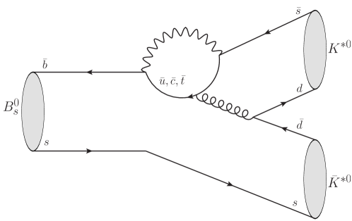
Figure 1: Leading-order SM Feynman diagram of the ${{{B}^{0}_{s}}\rightarrow{{K}^{*0}}{{\kern 1.99997pt\overline{\kern-1.99997ptK}{}}{}^{*0}}}$ decay.

The decay ${{{B}^{0}_{s}}\rightarrow{{K}^{*0}}{{\kern 1.99997pt\overline{\kern-1.99997ptK}{}}{}^{*0}}}$, with ${{K}^{*0}}\rightarrow K^{+}\pi^{-}$ and ${{\kern 1.99997pt\overline{\kern-1.99997ptK}{}}{}^{*0}}\rightarrow K^{-}\pi^{+}$, was first observed by the LHCb collaboration, based on $pp$ collision data corresponding to an integrated luminosity of $35\mbox{\,pb}^{-1}$ at a centre-of-mass energy $\sqrt{s}=7\mathrm{\,Te\kern-1.00006ptV}$ [13]. A branching fraction and a final-state polarisation analysis were reported. An updated analysis of the ${{{B}^{0}_{s}}\rightarrow({{K}^{+}}{{\pi}^{-}})({{K}^{-}}{{\pi}^{+}})}$ decay was performed by LHCb using $1.0$$\mbox{\,fb}^{-1}$ of data at $\sqrt{s}=7\mathrm{\,Te\kern-1.00006ptV}$ [14]. In both analyses, the invariant mass of the two $K\pi$ pairs was restricted to a window of $\pm 150$${\mathrm{\,Me\kern-1.00006ptV\!/}c^{2}}$ around the known ${K}^{*0}$ mass. This publication reports the first decay-time-dependent amplitude analysis of ${{{B}^{0}_{s}}\rightarrow({{K}^{+}}{{\pi}^{-}})({{K}^{-}}{{\pi}^{+}})}$ decays using a $K\pi$ mass window that extends from 750 to 1600${\mathrm{\,Me\kern-1.00006ptV\!/}c^{2}}$, approximately corresponding to the region between the $K\pi$ production threshold and the ${{D}^{0}}\rightarrow{{K}^{-}}{{\pi}^{+}}$ resonance. At the current level of sensitivity, the assumption of common $C\!P$-violating parameters for the contributing amplitudes is appropriate. Consequently, such a wide window provides a four-fold increase of the signal sample size with respect to the narrow window of $150{\mathrm{\,Me\kern-1.00006ptV\!/}c^{2}}$ around the ${K}^{*0}$ mass. The analysis uses $pp$ collision data collected by LHCb in 2011 and 2012 at $\sqrt{s}=7$ and $8\mathrm{\,Te\kern-1.00006ptV}$, corresponding to an integrated luminosity of $3.0\mbox{\,fb}^{-1}$. In this study, nine different quasi-two-body decay channels are considered, corresponding to the different possible combinations of $K\pi$ pairs with spin 0, 1 or 2. Additional contributions were studied and found to be negligible in the phase-space region considered in this analysis. The $K\pi$ spectrum is dominated by the $K_{0}^{*}(800)^{0}$, ${K}_{0}^{*}(1430)^{0}$, ${K}^{*}(892)^{0}$ and ${K}_{2}^{*}(1430)^{0}$ resonances. Angular momentum conservation in the decay allows for one single amplitude in modes involving at least one scalar $K\pi$ pair, three amplitudes for vector-vector or vector-tensor decays and five amplitudes for a tensor-tensor decay. These possibilities are listed in Table 1. There is a physical difference between decay pairs of the form scalar-vector and vector-scalar. Namely, in the used convention, the spectator quark from the $B_{s}^{0}$ decay (see Fig. 1) always ends up in the second $K\pi$ pair. The $C\!P$-averaged fractions of the contributing amplitudes, $f_{i}$, as well as their strong-phase differences, $\delta_{i}$, are determined together with the $C\!P$-violating weak phase $\phi_{s}^{{d}{\overline{d}}}$ and a parameter that accounts for the amount of $C\!P$ violation in decay, $|\lambda|$. This is the first time that the weak phase in ${b}\rightarrow{d}{\overline{d}}{s}$ transitions has been measured. It is also the first time that the tensor components in the $(K^{+}\pi^{-})(K^{-}\pi^{+})$ system have been studied.

Table 1: Quasi-two-body decay channels and corresponding polarisation amplitudes contributing to the ${{{B}^{0}_{s}}\rightarrow({{K}^{+}}{{\pi}^{-}})({{K}^{-}}{{\pi}^{+}})}$ final state in the $K\pi$ mass window from 750 to 1600${\mathrm{\,Me\kern-1.00006ptV\!/}c^{2}}$. The different contributions are identified by the spin $j_{1}$ ($j_{2}$) of the $K^{+}\pi^{-}$ ($K^{-}\pi^{+}$) pair and the helicity $h$. In cases where more than one amplitude contributes, the polarisations are defined as being longitudinal, parallel, or perpendicular, which are then denoted by $0$, $\parallel$ and $\perp$ respectively, following the definitions given in Ref. [15]. The subscripts 1 and 2 in the parallel and perpendicular helicities of the tensor-tensor component denote different spin states leading to a parallel or a perpendicular configuration, as discussed in Appendix A.

Decay	Mode	$j_{1}$	$j_{2}$	Allowed values of $h$	Number of amplitudes
${{B}^{0}_{s}}\rightarrow(K^{+}\pi^{-})^{*}_{0}(K^{-}\pi^{+})^{*}_{0}$	scalar-scalar	0	0	0	1
${{B}^{0}_{s}}\rightarrow(K^{+}\pi^{-})^{*}_{0}{{\kern 1.99997pt\overline{\kern-1.99997ptK}{}}{}^{*}(892)^{0}}$	scalar-vector	0	1	0	1
${{B}^{0}_{s}}\rightarrow{{K}^{*}(892)^{0}}(K^{-}\pi^{+})^{*}_{0}$	vector-scalar	1	0	0	1
${{B}^{0}_{s}}\rightarrow(K^{+}\pi^{-})^{*}_{0}{{\kern 1.99997pt\overline{\kern-1.99997ptK}{}}{}_{2}^{*}(1430)^{0}}$	scalar-tensor	0	2	0	1
${{B}^{0}_{s}}\rightarrow{{K}_{2}^{*}(1430)^{0}}(K^{-}\pi^{+})^{*}_{0}$	tensor-scalar	2	0	0	1
${{B}^{0}_{s}}\rightarrow{{K}^{*}(892)^{0}}{{\kern 1.99997pt\overline{\kern-1.99997ptK}{}}{}^{*}(892)^{0}}$	vector-vector	1	1	0, $\parallel$, $\perp$	3
${{B}^{0}_{s}}\rightarrow{{K}^{*}(892)^{0}}{{\kern 1.99997pt\overline{\kern-1.99997ptK}{}}{}_{2}^{*}(1430)^{0}}$	vector-tensor	1	2	0, $\parallel$, $\perp$	3
${{B}^{0}_{s}}\rightarrow{{K}_{2}^{*}(1430)^{0}}{{\kern 1.99997pt\overline{\kern-1.99997ptK}{}}{}^{*}(892)^{0}}$	tensor-vector	2	1	0, $\parallel$, $\perp$	3
${{B}^{0}_{s}}\rightarrow{{K}_{2}^{*}(1430)^{0}}{{\kern 1.99997pt\overline{\kern-1.99997ptK}{}}{}_{2}^{*}(1430)^{0}}$	tensor-tensor	2	2	0, $\parallel_{1}$, $\perp_{1}$, $\parallel_{2}$, $\perp_{2}$	5

2 Phenomenology

The phenomenon of quark mixing means that a ${B}^{0}_{s}$ meson can oscillate into its antiparticle equivalent, ${\kern 1.79993pt\overline{\kern-1.79993ptB}{}}{}^{0}_{s}$. Consequently, the physical states, $B^{0}_{s,\rm{H}}$ (heavy) and $B^{0}_{s,\rm{L}}$ (light), which have mass and decay width differences defined by $\Delta m_{s}=m_{B^{0}_{s,\rm{H}}}-m_{B^{0}_{s,\rm{L}}}$ and $\Delta\Gamma_{s}=\Gamma_{B^{0}_{s,\rm{L}}}-\Gamma_{B^{0}_{s,\rm{H}}}$, respectively, are admixtures of the flavour eigenstates such that

$$B^{0}_{s,\rm{H}}=p{{B}^{0}_{s}}+q{{\kern 1.79993pt\overline{\kern-1.79993ptB}{}}{}^{0}_{s}}\;\;\;\;\;\mathrm{and}\;\;\;\;\;B^{0}_{s,\rm{L}}=p{{B}^{0}_{s}}-q{{\kern 1.79993pt\overline{\kern-1.79993ptB}{}}{}^{0}_{s}},$$ (1)

where $p$ and $q$ are complex coefficients that satisfy $|p|^{2}+|q|^{2}=1$. The time evolution of the initially pure flavour eigenstates at $t=0$, $|{{B}^{0}_{s}}(0)\rangle$ and $|{{\kern 1.79993pt\overline{\kern-1.79993ptB}{}}{}^{0}_{s}}(0)\rangle$, is described by

$$|{{B}^{0}_{s}}(t)\rangle =g_{+}(t)|{{B}^{0}_{s}}(0)\rangle+\frac{q}{p}g_{-}(t)|{{\kern 1.79993pt\overline{\kern-1.79993ptB}{}}{}^{0}_{s}}(0)\rangle,$$ (2)

$$|{{\kern 1.79993pt\overline{\kern-1.79993ptB}{}}{}^{0}_{s}}(t)\rangle =\frac{p}{q}g_{-}(t)|{{B}^{0}_{s}}(0)\rangle+g_{+}(t)|{{\kern 1.79993pt\overline{\kern-1.79993ptB}{}}{}^{0}_{s}}(0)\rangle,$$

where the decay-time-dependent functions $g_{\pm}(t)$ are given by

$$g_{\pm}(t)=\frac{1}{2}e^{-im_{s}t}e^{-\frac{\Gamma_{s}}{2}t}\left(e^{i\frac{\Delta m_{s}}{2}t}e^{-\frac{\Delta\Gamma_{s}}{4}t}\pm e^{-i\frac{\Delta m_{s}}{2}t}e^{\frac{\Delta\Gamma_{s}}{4}t}\right),$$ (3)

with $m_{s}$ and $\Gamma_{s}$ being the average mass and width of the $B^{0}_{s,\rm{H}}$ and $B^{0}_{s,\rm{L}}$ states. Negligible $C\!P$ violation in mixing is assumed in this analysis, leading to the parameterisation $q/p=e^{-i\phi_{\rm M}}$, where $\phi_{\rm M}$ is the ${B}^{0}_{s}$–${\kern 1.79993pt\overline{\kern-1.79993ptB}{}}{}^{0}_{s}$ mixing phase. The total decay amplitude of the flavour eigenstates at $t=0$ into the final state $f=({{K}^{+}}{{\pi}^{-}})({{K}^{-}}{{\pi}^{+}})$, denoted by $\langle f|{{B}^{0}_{s}}(0)\rangle$ and $\langle f|{{\kern 1.79993pt\overline{\kern-1.79993ptB}{}}{}^{0}_{s}}(0)\rangle$, is a coherent sum of scalar-scalar (SS), scalar-vector (SV), vector-scalar (VS), scalar-tensor (ST), tensor-scalar (TS), vector-vector (VV), vector-tensor (VT), tensor-vector (TV) and tensor-tensor (TT) contributions. The quantum numbers used to label the $({{K}^{+}}{{\pi}^{-}})({{K}^{-}}{{\pi}^{+}})$ final states are the spin $j_{1}$ ($j_{2}$) of the $K^{+}\pi^{-}$ ($K^{-}\pi^{+}$) pair and the helicity $h$. The vector component is represented in this analysis by the $K^{*0}$ meson, since this resonance is found to be largely dominant in this spin configuration. Potential contributions from the $K_{1}^{*}(1410)^{0}$ and $K_{1}^{*}(1680)^{0}$ resonances are considered as sources of systematic uncertainty. For the tensor case, only the $K_{2}^{*}(1430)^{0}$ resonance contributes in the considered $K\pi$ mass window. The scalar component, denoted in this paper by $(K\pi)_{0}^{*}$ requires a more careful treatment. It can have contributions from the $K_{0}^{*}(800)^{0}$ and $K_{0}^{*}(1430)^{0}$ resonances and from a nonresonant $K\pi$ component. The parameterisation of the $K\pi$ invariant mass spectrum for the scalar contribution is explained later in this section. All of the considered decay modes, together with the quantum numbers for the corresponding amplitudes, are shown in Table 1. In order to separate components with different $C\!P$ eigenvalues, $\eta_{h}^{j_{1}j_{2}}=\pm 1$, the differential decay rate is expressed as a function of three angles and the two $K\pi$ invariant masses. The angles $\theta_{1}$, $\theta_{2}$ and $\varphi$, are written in the helicity basis and defined according to the diagram shown in Fig. 2. The invariant mass of the ${K}^{+}$ ${\pi}^{-}$ pair is denoted as $m_{1}$, while that of the ${K}^{-}$ ${\pi}^{+}$ pair as $m_{2}$. The symbol $\Omega$ is used to represent all three angles and the two invariant masses, $\Omega=(m_{1},m_{2},\cos\theta_{1},\cos\theta_{2},\varphi)$.

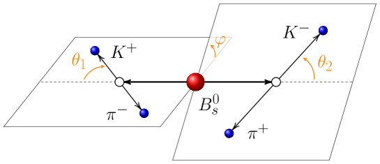
Figure 2: Graphical definition of the angles in the helicity basis. Taking the example of a ${{B}^{0}_{s}}\rightarrow Q_{1}Q_{2}$ decay (this analysis uses ${{B}^{0}_{s}}\rightarrow SS$, ${{B}^{0}_{s}}\rightarrow SV$, ${{B}^{0}_{s}}\rightarrow VS$, ${{B}^{0}_{s}}\rightarrow VV$, ${{B}^{0}_{s}}\rightarrow ST$, ${{B}^{0}_{s}}\rightarrow TS$, ${{B}^{0}_{s}}\rightarrow VT$, ${{B}^{0}_{s}}\rightarrow TV$ and ${{B}^{0}_{s}}\rightarrow TT$), with each final-state quasi-two-body meson decaying to pseudoscalars ($Q_{1}\rightarrow K^{+}\pi^{-}$ and $Q_{2}\rightarrow K^{-}\pi^{+}$), $\theta_{1}$ ($\theta_{2}$) is defined as the angle between the directions of motion of $K^{+}$ ($K^{-}$) in the $Q_{1}$ ($Q_{2}$) rest frame and $Q_{1}$ ($Q_{2}$) in the ${B}^{0}_{s}$ rest frame, and $\varphi$ as the angle between the plane defined by $K^{+}\pi^{-}$ and the plane defined by $K^{-}\pi^{+}$ in the ${B}^{0}_{s}$ rest frame.

Summing over the possible states and using the partial wave formalism, the decay amplitudes at $t=0$ can be written as

$$\langle f|{{B}^{0}_{s}}(0)\rangle(\Omega) =\sum_{j_{1},j_{2},h}\mathcal{A}_{h}^{j_{1}j_{2}}\Theta^{j_{1}j_{2}}_{h}(\cos{\theta_{1}},\cos{\theta_{2}},\varphi)\mathcal{H}_{h}^{j_{1}j_{2}}(m_{1},m_{2}),$$ (4)

$$\langle f|{{\kern 1.79993pt\overline{\kern-1.79993ptB}{}}{}^{0}_{s}}(0)\rangle(\Omega) =\sum_{j_{1},j_{2},h}\eta_{h}^{j_{1}j_{2}}\overline{\mathcal{A}}_{h}^{j_{1}j_{2}}\Theta^{j_{1}j_{2}}_{h}(\cos{\theta_{1}},\cos{\theta_{2}},\varphi)\mathcal{H}_{h}^{j_{1}j_{2}}(m_{1},m_{2}).$$

The complex parameters $\mathcal{A}_{h}^{j_{1}j_{2}}$ and $\overline{\mathcal{A}}_{h}^{j_{1}j_{2}}$ contain the physics of the decays to the final states with $j_{1}$, $j_{2}$ and $h$ as defined in Table 1. The angular terms, $\Theta_{h}^{j_{1}j_{2}}$, are built from combinations of spherical harmonics as shown in Appendix A. The $\eta_{h}^{j_{1}j_{2}}$ factor is equal to $(-1)^{j_{1}+j_{2}}\,\eta_{h}$, where $\eta_{h}=1$ for $h\in\{0,\parallel,\parallel_{1},\parallel_{2}\}$ and $\eta_{h}=-1$ for $h\in\{\perp,\perp_{1},\perp_{2}\}$. The mass-dependent terms are parameterised as

$$\mathcal{H}_{h}^{j_{1}j_{2}}(m_{1},m_{2})=\mathcal{F}_{h}^{j_{1}j_{2}}(m_{1},m_{2})\mathcal{M}_{j_{1}}(m_{1})\mathcal{M}_{j_{2}}(m_{2}),$$ (5)

where $\mathcal{F}_{h}^{j_{1}j_{2}}(m_{1},m_{2})$ is the Blatt–Weisskopf angular-momentum centrifugal-barrier factor [16] and $\mathcal{M}_{j}$ describes the shape of the $K\pi$ invariant mass of a $K\pi$ pair with spin $j$. Relativistic Breit–Wigner functions of spin 1 and 2, parameterising the ${K}^{*0}$ and the ${K}_{2}^{*}(1430)^{0}$ resonances, are used for $\mathcal{M}_{1}$ and $\mathcal{M}_{2}$, respectively. The parameterisation of $\mathcal{M}_{0}$ is based on the phenomenological $S$-wave scattering amplitude of isospin $1/2$ presented in Ref. [17]. Since only the phase evolution of $\mathcal{M}_{0}$ is linked to that of the scattering amplitude (by virtue of Watson’s theorem [18]), its modulus is parameterised with a fourth-order polynomial whose coefficients are determined in the final fit to data. Details of this parameterisation can be found in Appendix B. The normalisation condition for the mass-dependent terms is

$$\int dm_{1}\int dm_{2}\;|\mathcal{H}_{h}^{j_{1}j_{2}}(m_{1},m_{2})|^{2}\Phi_{4}(m_{1},m_{2})=1,$$ (6)

where $\Phi_{4}$ is the four-body phase-space factor. The phase of $\mathcal{H}_{h}^{j_{1}j_{2}}(m_{1},m_{2})$ is set to 0 at $m_{1}=m_{2}=M({{K}^{*0}})$, where $M({{K}^{*0}})$ is the mass of the ${{K}^{*0}}$ state [15], in order to normalise the relative global phases of the $K\pi$ mass-dependent amplitudes. The $C\!P$-violating effects are assumed to be the same for all of the modes under study. Consequently, the value of $\phi_{s}^{{d}{\overline{d}}}$ and $|\lambda|$ determined in this article is effectively an average over the various channels considered in Table 1. Within this approach, the physical amplitudes $\mathcal{A}_{h}^{j_{1}j_{2}}$ and $\overline{\mathcal{A}}_{h}^{j_{1}j_{2}}$ in Eq. (4) can be separated into a $C\!P$-averaged complex amplitude, $A_{h}^{j_{1}j_{2}}$, a direct $C\!P$ asymmetry, $\Delta^{{C\!P}}_{\rm dir}=(|\overline{\mathcal{A}_{h}^{j_{1}j_{2}}}|^{2}-|\mathcal{A}_{h}^{j_{1}j_{2}}|^{2})/(|\overline{\mathcal{A}_{h}^{j_{1}j_{2}}}|^{2}+|\mathcal{A}_{h}^{j_{1}j_{2}}|^{2})$, and a $C\!P$-violating weak phase in the decay, $\phi_{\rm D}$, as

$$\mathcal{A}_{h}^{j_{1}j_{2}} =\sqrt{1-\Delta^{{C\!P}}_{\rm dir}}e^{-i\phi_{\rm D}}A_{h}^{j_{1}j_{2}},$$ (7)

$$\overline{\mathcal{A}}_{h}^{j_{2}j_{1}}=\overline{\mathcal{A}_{h}^{j_{1}j_{2}}} =\sqrt{1+\Delta^{{C\!P}}_{\rm dir}}e^{i\phi_{\rm D}}A_{h}^{j_{1}j_{2}}.$$

In the expressions above the $C\!P$ transformation also changes $j_{1}j_{2}$ to $j_{2}j_{1}$. The total $C\!P$-violating phase associated to the interference between mixing and decay is given by $\phi_{s}^{{d}{\overline{d}}}=\phi_{\rm M}-2\phi_{\rm D}$ and its determination is the main goal of this analysis. In the SM the size of $\phi_{s}^{{d}{\overline{d}}}$ is expected to be small due to an almost exact cancellation in the values of $\phi_{\rm M}$ and $2\phi_{\rm D}$ [5]. The parameter $|\lambda|$ is defined in terms of the direct $C\!P$ asymmetry by

$$|\lambda|=\frac{\sqrt{1+\Delta^{{C\!P}}_{\rm dir}}}{\sqrt{1-\Delta^{{C\!P}}_{\rm dir}}}.$$ (8)

3 Detector and simulation

The LHCb detector [19, 20] is a single-arm forward spectrometer covering the pseudorapidity range between $2$ and $5$, designed for the study of particles containing $b$ or $c$ quarks. The detector includes a high-precision tracking system consisting of a silicon-strip vertex detector surrounding the $pp$ interaction region, a large-area silicon-strip detector located upstream of a dipole magnet with a bending power of about $4{\mathrm{\,Tm}}$, and three stations of silicon-strip detectors and straw drift tubes placed downstream of the magnet. The tracking system provides a measurement of momentum, $p$, of charged particles with relative uncertainty that varies from 0.5% at low momentum to 1.0% at 200${\mathrm{\,Ge\kern-1.00006ptV\!/}c}$. The minimum distance of a track to a primary vertex (PV), the impact parameter (IP), is measured with resolution of $(15+29/\mbox{$p_{\mathrm{T}}$}){\,\upmu\mathrm{m}}$, where $p_{\mathrm{T}}$ is the component of the momentum transverse to the beam, in ${\mathrm{\,Ge\kern-1.00006ptV\!/}c}$. Different types of charged hadrons are distinguished using information from two ring-imaging Cherenkov (RICH) detectors. Photons, electrons and hadrons are identified by a calorimeter system consisting of scintillating-pad and preshower detectors, an electromagnetic calorimeter and a hadronic calorimeter. Muons are identified by a system composed of alternating layers of iron and multiwire proportional chambers. The online event selection is performed by a trigger, which consists of a hardware stage, based on information from the calorimeter and muon systems, followed by a software stage, which applies a full event reconstruction. At the hardware trigger stage, events are required to contain a muon with high $p_{\mathrm{T}}$ or a hadron, photon or electron with high transverse energy in the calorimeters. The software trigger requires a two-, three- or four-track secondary vertex with significant displacement from the primary $pp$ interaction vertices. At least one charged particle must have transverse momentum $\mbox{$p_{\mathrm{T}}$}>1.7{\mathrm{\,Ge\kern-1.00006ptV\!/}c}$ and be inconsistent with originating from a PV. A multivariate algorithm [21] is used for the identification of secondary vertices consistent with the decay of a $b$ hadron. Simulated samples of resonant ${{{B}^{0}_{s}}\rightarrow{{K}^{*0}}{{\kern 1.99997pt\overline{\kern-1.99997ptK}{}}{}^{*0}}}$, ${{{B}^{0}_{s}}\rightarrow{{K}^{*0}}{{\kern 1.99997pt\overline{\kern-1.99997ptK}{}}{}_{0}^{*}(1430)^{0}}}$ and ${{{B}^{0}_{s}}\rightarrow{{K}_{0}^{*}(1430)^{0}}{{\kern 1.99997pt\overline{\kern-1.99997ptK}{}}{}_{0}^{*}(1430)^{0}}}$ decays, as well as phase-space ${{{B}^{0}_{s}}\rightarrow{{K}^{+}}{{\pi}^{-}}{{K}^{-}}{{\pi}^{+}}}$ decays, are used to study the signal. Simulated samples of ${{{B}^{0}}\rightarrow{{K}^{*0}}{{\kern 1.99997pt\overline{\kern-1.99997ptK}{}}{}^{*0}}}$, ${{{B}^{0}}\rightarrow{{K}^{*0}}{{\rho}^{0}}}$, ${{{B}^{0}}\rightarrow{{K}^{*0}}\phi}$ and ${{{\mathchar 28931\relax}^{0}_{b}}\rightarrow({p}{{K}^{-}})({{\pi}^{+}}{{\pi}^{-}})}$ are created to study peaking backgrounds. In the simulation, $pp$ collisions are generated using Pythia [22] with a specific LHCb configuration [23]. Decays of particles are described by EvtGen [24], in which final-state radiation is generated using Photos [25]. The interaction of the generated particles with the detector, and its response, are implemented using the Geant4 toolkit [26, *Agostinelli:2002hh] as described in Ref. [28].

4 Signal candidate selection

Events passing the trigger are required to satisfy requirements on the fit quality of the ${B}^{0}_{s}$ decay vertex as well as the $p_{\mathrm{T}}$ and $\chi^{2}_{\text{IP}}$ of each track, where $\chi^{2}_{\text{IP}}$ is defined as the difference between the $\chi^{2}$ of the secondary vertex reconstructed with and without the track under consideration. The tracks are assigned as kaon or pion candidates using particle identification information from the RICH detectors by requiring that the likelihood for the kaon hypothesis is larger than that for the pion hypothesis and vice versa. In addition, the $p_{\mathrm{T}}$ of each $K\pi$ pair is required to be larger than $500$${\mathrm{\,Me\kern-1.00006ptV\!/}c}$, the reconstructed mass of each $K\pi$ pair is required to be within the range $750\leq m(K\pi)\leq 1600$${\mathrm{\,Me\kern-1.00006ptV\!/}c^{2}}$ and the reconstructed mass of the ${B}^{0}_{s}$ candidate is required to be within the range $5000\leq m({{K}^{+}}{{\pi}^{-}}{{K}^{-}}{{\pi}^{+}})\leq 5800$${\mathrm{\,Me\kern-1.00006ptV\!/}c^{2}}$. A boosted decision tree (BDT) algorithm [29, 30] is trained to reject combinatorial background, where at least one of the final-state tracks originates from a different decay or directly from the PV. The signal is represented in the BDT training with simulated ${{B}^{0}_{s}}\rightarrow{{K}^{*0}}{{\kern 1.99997pt\overline{\kern-1.99997ptK}{}}{}^{*0}}$ candidates, satisfying the same requirements as the data, while selected data candidates in the four-body invariant mass sideband, $5600\leq m({{K}^{+}}{{\pi}^{-}}{{K}^{-}}{{\pi}^{+}})\leq 5800$${\mathrm{\,Me\kern-1.00006ptV\!/}c^{2}}$, are used to represent the background. The input variables employed in the training are kinematic and geometric quantities associated with the four final-state tracks, the two $K\pi$ candidates and the ${B}^{0}_{s}$ candidate. The features used to train the BDT response are chosen to minimise any correlation with the ${B}^{0}_{s}$ and two $K\pi$ pair invariant masses. Separate trainings are performed for the data samples collected in 2011 and 2012, due to the different data-taking conditions. The $k$-fold cross-validation method [31], with $k=4$, is used to increase the training statistics while reducing the risk of overtraining. The requirement on the BDT response is optimized by maximising the metric $N_{\rm S}/\sqrt{N_{\rm S}+N_{\rm B}}$, where $N_{\rm S}$ is the estimated number of signal candidates after selection and $N_{\rm B}$ is the estimated number of combinatorial background candidates within $\pm 60{\mathrm{\,Me\kern-1.00006ptV\!/}c^{2}}$ of the known ${B}^{0}_{s}$ mass [15]. The BDT requirement is 95% efficient for simulated signal candidates and rejects 70% of the combinatorial background. After applying the BDT requirement, specific background contributions containing two real oppositely charged kaons and two real oppositely charged pions are removed by mass vetoes on the two- and three-body invariant masses. Candidates are removed if they fulfill either $m({{K}^{+}}{{K}^{-}}{{\pi}^{\pm}})<2100$${\mathrm{\,Me\kern-1.00006ptV\!/}c^{2}}$ or $m({{K}^{+}}{{K}^{-}})$ within 30${\mathrm{\,Me\kern-1.00006ptV\!/}c^{2}}$ of the known ${D}^{0}$ mass [15]. Sources of peaking background in which one of the final-state tracks is misidentified are suppressed by introducing further particle identification requirements. The particle identification quantities make use of information from the RICH detectors and are calibrated using ${{D}^{*+}}\rightarrow{{D}^{0}}{{\pi}^{+}}$ and ${{\mathchar 28931\relax}^{0}_{b}}\rightarrow{{\mathchar 28931\relax}^{+}_{c}}{\mu^{-}}{{\overline{\nu}}_{\mu}}$ decays in data. These requirements significantly reduce contributions from ${{B}^{0}}\rightarrow{{\rho}^{0}}{{K}^{*0}}$, ${{B}^{0}}\rightarrow\phi{{K}^{*0}}$ and ${{\mathchar 28931\relax}^{0}_{b}}\rightarrow{p}{{\pi}^{-}}{{K}^{-}}{{\pi}^{+}}$ in which a pion or proton is misidentified as a kaon, or a kaon is misidentified as a pion. In addition, there are specific extra particle identification requirements for candidates whose reconstructed mass falls within $\pm 30$${\mathrm{\,Me\kern-1.00006ptV\!/}c^{2}}$ of the known ${B}^{0}$ or ${\mathchar 28931\relax}^{0}_{b}$ mass under the relevant mass-hypothesis change ($K\rightarrow{p}$, $K\rightarrow\pi$ or $\pi\rightarrow K$). These requirements remove 40% of the simulated signal but almost all of the simulated background: 80% of ${{B}^{0}}\rightarrow\phi{{K}^{*0}}$, 96% of ${{B}^{0}}\rightarrow\rho{{K}^{*0}}$ and 88% of ${{\mathchar 28931\relax}^{0}_{b}}\rightarrow{p}{{\pi}^{-}}{{K}^{-}}{{\pi}^{+}}$ events. Subsequently, each of these background components is found to have a small effect on the signal determination. After all of the selection criteria have been imposed, 1.4% of selected events contain multiple candidates, from which one is randomly selected. A fit to the four-body invariant mass distribution is performed in order to determine a set of signal weights, obtained using the sPlot procedure [32], which allows the decay-time-dependent $C\!P$ fit to be performed on a sample that represents only the signal. For the invariant mass fit the ${{B}^{0}_{s}}\rightarrow({{K}^{+}}{{\pi}^{-}})({{K}^{-}}{{\pi}^{+}})$ signal and the peaking background components ${{B}^{0}}\rightarrow({{K}^{+}}{{\pi}^{-}})({{K}^{-}}{{\pi}^{+}})$, $B^{0}_{(s)}\rightarrow({{K}^{+}}{{K}^{-}})({{K}^{-}}{{\pi}^{+}})$, ${{B}^{0}}\rightarrow({{\pi}^{+}}{{\pi}^{-}})({{K}^{-}}{{\pi}^{+}})$ and ${{\mathchar 28931\relax}^{0}_{b}}\rightarrow({p}{{\pi}^{-}})({{K}^{-}}{{\pi}^{+}})$ are modelled as Ipatia functions [33] in which the tail parameters are fixed to values obtained from fits to the simulated samples. The mass difference between the ${B}^{0}_{s}$ and ${B}^{0}$ mesons is fixed to its known value whilst the mean of the ${B}^{0}_{s}$ component, as well as the width of both the ${B}^{0}$ and ${B}^{0}_{s}$ components, are allowed to vary freely. The yields of the ${{{{B}^{0}_{s}}\rightarrow({{K}^{+}}{{\pi}^{-}})({{K}^{-}}{{\pi}^{+}})}}$, ${{{B}^{0}}\rightarrow({{K}^{+}}{{\pi}^{-}})({{K}^{-}}{{\pi}^{+}})}$ and ${{{B}^{0}}\rightarrow({{K}^{+}}{{K}^{-}})({{K}^{-}}{{\pi}^{+}})}$ components are allowed to freely vary, whilst the yields of the other components are Gaussian constrained to values relative to the known ${{B}^{0}}\rightarrow({{K}^{+}}{{K}^{-}})({{K}^{-}}{{\pi}^{+}})$ branching fraction taking into account the relevant production fractions [34] and reconstruction efficiencies. There is an additional background contribution in the low-mass region from partially reconstructed $b$-hadron decays in which a pion is missed in the final state. This component is modelled as an ARGUS function [35] convolved with a Gaussian mass resolution function. The ARGUS cutoff parameter is fixed to the fitted ${B}^{0}_{s}$ mass minus the neutral pion mass, with the other parameters and yield allowed to vary. The combinatorial background is modelled as an exponential function whose shape parameter and yield are allowed to vary. The result of the four-body invariant mass fit, which is used to obtain the sPlot signal weights, is shown in Fig. 3. The two $K\pi$ pair invariant masses, with the signal weights applied, are shown in Fig. 4. The resulting yields of the various fit components are shown in Table 2.

Table 2: Yields of the signal decay and the various background components considered in the four-body invariant mass fit. The uncertainties are statistical only. The signal region is defined as $\pm 60$${\mathrm{\,Me\kern-1.00006ptV\!/}c^{2}}$ from the known ${B}^{0}_{s}$ meson mass [15].

Channel	Yield			Yield in Signal Region
${{B}^{0}_{s}}\rightarrow({{K}^{+}}{{\pi}^{-}})({{K}^{-}}{{\pi}^{+}})$	6080	$\pm$	83	6004
${{B}^{0}}\rightarrow({{K}^{+}}{{\pi}^{-}})({{K}^{-}}{{\pi}^{+}})$	1013	$\pm$	49	103
${{B}^{0}}\rightarrow({{K}^{+}}{{\pi}^{-}})({{K}^{-}}{{K}^{+}})$	281	$\pm$	47	1
${{B}^{0}_{s}}\rightarrow({{K}^{+}}{{\pi}^{-}})({{K}^{-}}{{K}^{+}})$	8	$\pm$	3	4
${{B}^{0}}\rightarrow({{K}^{+}}{{\pi}^{-}})({{\pi}^{-}}{{\pi}^{+}})$	57	$\pm$	13	33
${{\mathchar 28931\relax}^{0}_{b}}\rightarrow({p}{{\pi}^{-}})({{K}^{-}}{{\pi}^{+}})$	44	$\pm$	10	13
Partially reconstructed	2580	$\pm$	151	0
Combinatorial	2810	$\pm$	214	372

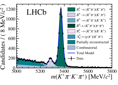
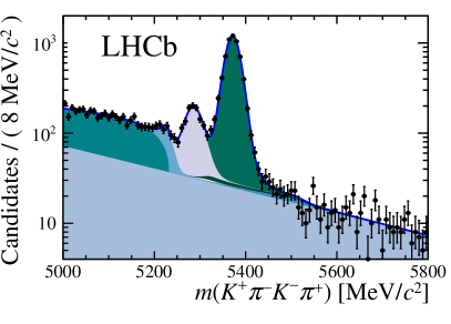
Figure 3: Four-body invariant mass distribution on a (left) linear and (right) logarithmic scale superimposed with the mass fit model.

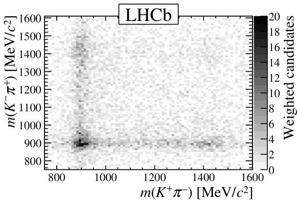
Figure 4: Distribution of the two $(K\pi)$ pair invariant masses, with the signal weights applied, after all of the selection requirements.

5 Flavour tagging

At the LHC, $b$ quarks are predominantly produced in ${b}{\overline{b}}$ pairs. This analysis focuses on events where one of the quarks hadronises to produce the ${B}^{0}_{s}$ meson while the other quark hadronises and decays independently. Taking advantage of this effect, two types of tagging algorithms aimed at identifying the $b$-quark flavour at production time are used in this analysis: same-side (SS) taggers, based on information from accompanying particles associated with the signal ${B}^{0}_{s}$ hadronisation process; and opposite-side (OS) taggers, based on particles produced in the decay of the other $b$ quark. This analysis uses the neural-network-based SS-kaon tagging algorithm presented in Ref. [36]; and the combination of OS tagging algorithms explained in Ref. [37], based on information from $b$-hadron decays to electrons, muons or kaons and the total charge of tracks that form a vertex. Both the SS and OS tagging algorithms provide for each event a tagging decision, $\mathfrak{q}$, and an estimated mistag probability, $\eta_{\rm tag}$. The tagging decision takes the value $1$ for ${B}^{0}_{s}$, $-1$ for ${\kern 1.79993pt\overline{\kern-1.79993ptB}{}}{}^{0}_{s}$ and $0$ for untagged. To obtain the calibrated mistag probability for a ${B}^{0}_{s}$ (${\kern 1.79993pt\overline{\kern-1.79993ptB}{}}{}^{0}_{s}$) meson, $\omega$ ($\bar{\omega}$), the estimated probability is calibrated on several flavour-specific control channels. The following linear functions are used in the calibration

$$\omega^{\rm X}(\eta_{\rm tag}^{\rm X}) =\left(p_{0}^{\rm X}+\frac{\Delta p_{0}^{\rm X}}{2}\right)+\left(p_{1}^{\rm X}+\frac{\Delta p_{1}^{\rm X}}{2}\right)(\eta_{\rm tag}^{\rm X}-\langle\eta_{\rm tag}^{\rm X}\rangle),$$ (9)

$$\bar{\omega}^{\rm X}(\eta_{\rm tag}^{\rm X}) =\left(p_{0}^{\rm X}-\frac{\Delta p_{0}^{\rm X}}{2}\right)+\left(p_{1}^{\rm X}-\frac{\Delta p_{1}^{\rm X}}{2}\right)(\eta_{\rm tag}^{\rm X}-\langle\eta_{\rm tag}^{\rm X}\rangle),$$

where $\rm X\in\{OS,SS\}$, $\langle\eta_{\rm tag}^{\rm X}\rangle$ is the mean $\eta_{\rm tag}^{\rm X}$ of the sample, $p_{0,1}^{\rm X}$ correspond to calibration parameters averaged over ${B}^{0}_{s}$ and ${\kern 1.79993pt\overline{\kern-1.79993ptB}{}}{}^{0}_{s}$, and $\Delta p_{0,1}^{\rm X}$ account for ${B}^{0}_{s}$ and ${\kern 1.79993pt\overline{\kern-1.79993ptB}{}}{}^{0}_{s}$ asymmetries in the calibration. Among other modes, the portability of the SS tagger calibration was checked on $B_{s}^{0}\rightarrow\phi\phi$ decays [36], which are kinematically similar to the considered signal mode. The tagging efficiency, $\epsilon_{\rm tag}$, denotes the fraction of candidates with a nonzero tagging decision. The tagging power of the sample, $\epsilon_{\rm eff}=\epsilon_{\rm tag}(1-2\langle\omega\rangle)^{2}$, characterises the tagging performance. Information from the SS and OS algorithms is combined on a per-event basis (see Eq. (13)) for the decay-time-dependent amplitude fit discussed in Sec. 7. The overall effective tagging power is found to be $(5.15\pm 0.14)\%$. The flavour-tagging performance is shown in Table 3. When separating the ${\kern 1.79993pt\overline{\kern-1.79993ptB}{}}{}^{0}_{s}$ and ${B}^{0}_{s}$ components at $t=0$, the value of the production asymmetry $A_{p}=[\sigma({{\kern 1.79993pt\overline{\kern-1.79993ptB}{}}{}^{0}_{s}})-\sigma({{B}^{0}_{s}})]/[\sigma({{\kern 1.79993pt\overline{\kern-1.79993ptB}{}}{}^{0}_{s}})+\sigma({{B}^{0}_{s}})]$, where $\sigma({{B}^{0}_{s}})$ ($\sigma({{\kern 1.79993pt\overline{\kern-1.79993ptB}{}}{}^{0}_{s}})$) is the production cross-section for the ${B}^{0}_{s}$ (${\kern 1.79993pt\overline{\kern-1.79993ptB}{}}{}^{0}_{s}$) meson, also has to be incorporated in the model. This asymmetry was measured by LHCb in $pp$ collisions at $\sqrt{s}=7$ TeV by means of a decay-time-dependent analysis of ${{B}^{0}_{s}}\rightarrow{{D}^{-}_{s}}{{\pi}^{+}}$ decays [38]. To correct for the different kinematics of ${{B}^{0}_{s}}\rightarrow{{D}^{-}_{s}}{{\pi}^{+}}$ and ${{{B}^{0}_{s}}\rightarrow({{K}^{+}}{{\pi}^{-}})({{K}^{-}}{{\pi}^{+}})}$ decays, a weighting in bins of ${B}^{0}_{s}$ transverse momentum and pseudorapidity is performed, yielding a value of $A_{p}=-0.005\pm 0.019$. No detection asymmetry need be considered in this analysis since the final state under consideration is charge symmetric.

Table 3: The flavour-tagging performance of the SS and OS tagging algorithms, as well as the combination of both, for the signal data sample used in the analysis. The quoted uncertainty includes both statistical and systematic contributions.

Tagging algorithm	$\epsilon_{\rm tag}$ [%]	$\epsilon_{\rm eff}$ [%]
SS	$62.0\pm 0.7$	$1.63\pm 0.21$
OS	$37.1\pm 0.7$	$3.70\pm 0.21$
Combination	$75.6\pm 0.6$	$5.15\pm 0.14$

6 Acceptance and resolution effects

The LHCb geometrical coverage and selection procedure induce acceptance effects that depend on the three decay angles, the $K\pi$ two-body invariant masses and the decay time. In addition, imperfect reconstruction gives rise to resolution effects. Any deviations caused by imperfect angular and mass resolution are small and are accounted for within the evaluation of systematic uncertainties (see Sec. 8). However, knowledge of the decay-time resolution is of key importance in the determination of $\phi_{s}^{{d}{\overline{d}}}$ and is consequently included in the decay-time-dependent fit. In this analysis, both acceptance and resolution effects are studied using samples of simulated events which have been weighted to match the data distributions in several important kinematic variables. In the description of the acceptance, the decay-time-dependent part is factorised with respect to the part that depends on the kinematic quantities, since they are found to be only $5\%$ correlated. The acceptance and the decay-time resolutions are determined from simulated events that contain an appropriate combination of the vector-vector ${{{B}^{0}_{s}}\rightarrow{{K}^{*0}}{{\kern 1.99997pt\overline{\kern-1.99997ptK}{}}{}^{*0}}}$ component with a sample of ${{B}^{0}_{s}}\rightarrow K^{+}\pi^{-}K^{-}\pi^{+}$ decays generated according to a phase-space distribution. This combination sufficiently populates the phase-space regions to represent the signal decay. To obtain the acceptance function, the simulated events are weighted by the inverse of the probability density function (PDF) used for generation (defined in terms of angles, masses and decay time). The decay-time acceptance is treated analytically and parameterised using cubic spline functions, following the procedure outlined in Ref. [39], with the number of knots chosen to be six. The effect of this choice is addressed as a systematic uncertainty in Sec. 8. The decay-time acceptance is shown in Fig. 5 (bottom right). The five-dimensional kinematic acceptance in angles and masses is included by using normalisation weights in the denominator of the PDF used in the fit to the data, following the procedure described in Ref. [40]. When visualising the fit results (see Fig. 7), the simulated events are weighted using the matrix element of the amplitude fit model. For illustrative purposes, some projections of the kinematic acceptance are shown in Fig. 5. In order to obtain the best possible sensitivity for the measurement of the $\phi_{s}^{{d}{\overline{d}}}$ phase, the time resolution is evaluated event by event, using the estimated decay-time uncertainty, $\delta_{t}$, obtained in the track reconstruction process. This variable is calibrated using the simulation sample described above to provide the per-event decay-time resolution, $\sigma_{t}$, using a linear relationship

$$\sigma_{t}(\delta_{t})=p_{0}^{\sigma_{t}}+p_{1}^{\sigma_{t}}(\delta_{t}-\langle\delta_{t}\rangle),$$ (10)

where $\langle\delta_{t}\rangle$ is the mean $\delta_{t}$ of the sample and $p_{(0,1)}^{\sigma_{t}}$ are the calibration parameters. During fitting, $\sigma_{t}$ is taken to be the width of a Gaussian resolution function which convolves the decay-time-dependent part of the total amplitude model. Figure 6 shows the relationship between the estimated decay-time uncertainty, $\delta_{t}$, and the calibrated per-event decay-time resolution, $\sigma_{t}$.

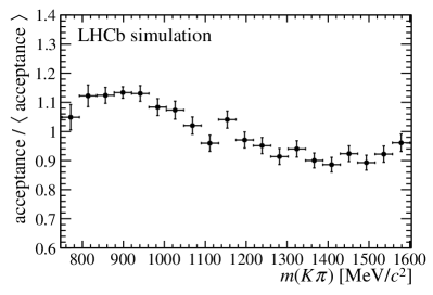
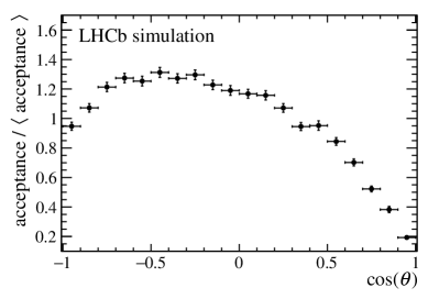
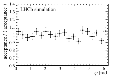
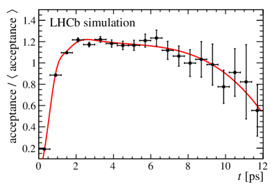
Figure 5: Kinematic acceptance and decay-time distributions evaluated with simulated vector-vector ${{{B}^{0}_{s}}\rightarrow{{K}^{*0}}{{\kern 1.99997pt\overline{\kern-1.99997ptK}{}}{}^{*0}}}$ and pure phase-space ${{{B}^{0}_{s}}\rightarrow({{K}^{+}}{{\pi}^{-}})({{K}^{-}}{{\pi}^{+}})}$ candidates scaled by the mean acceptance. In the bottom right plot the decay-time acceptance obtained from the simulated sample is shown as the black points and the parametric form of the acceptance obtained with cubic splines is shown as the red curve. In the other three plots the black points show the acceptance distribution for the masses and angles. The two $\cos\theta$ variables and the two $m(K\pi)$ masses have been averaged for the purpose of illustration. In the fit, the kinematic acceptance enters via the normalisation weights.

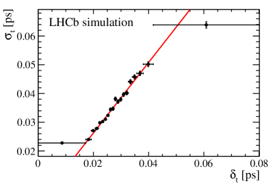
Figure 6: Per-event decay-time resolution, $\sigma_{t}$, versus the estimated per-event decay-time uncertainty, $\delta_{t}$, obtained from simulated samples containing both vector-vector resonant ${{{B}^{0}_{s}}\rightarrow{{K}^{*0}}{{\kern 1.99997pt\overline{\kern-1.99997ptK}{}}{}^{*0}}}$ and phase-space ${{{B}^{0}_{s}}\rightarrow{{K}^{+}}{{\pi}^{-}}{{K}^{-}}{{\pi}^{+}}}$ events.

7 Decay-time-dependent amplitude fit

The model used to fit the data is built by taking the squared moduli of the amplitudes $\langle f|{{B}^{0}_{s}}(t)\rangle$ and $\langle f|{{\kern 1.79993pt\overline{\kern-1.79993ptB}{}}{}^{0}_{s}}(t)\rangle$ introduced in Sec. 2, multiplying them by the four-body phase-space factor, incorporating the relevant flavour-tagging and production-asymmetry parameters, and including the acceptance and resolution factors obtained in Sec. 6. The observables $\eta_{\rm tag}^{\rm SS}$, $\eta_{\rm tag}^{\rm OS}$ and $\delta_{t}$ (introduced in Sec. 5 and Sec. 6) are treated as conditional variables. The effective normalised PDF can be written as

$$\text{PDF}(t,\Omega)=\frac{\sum_{\alpha=1}^{19}\sum_{\beta\leq\alpha}\Re e[K_{\alpha\beta}(t)F_{\alpha\beta}(\Omega)]}{\sum_{\alpha^{\prime}=1}^{19}\sum_{\beta^{\prime}\leq\alpha^{\prime}}\Re e[(\int dt^{\prime}\,K^{\rm untag}_{\alpha^{\prime}\beta^{\prime}}(t^{\prime})\epsilon_{t}(t^{\prime}))\xi_{\alpha^{\prime}\beta^{\prime}}]},$$ (11)

where the subscript $\alpha$ ($\beta$) represents the state labels $\{j_{1},j_{2},h\}$ ($\{j_{1}^{\prime},j_{2}^{\prime},h^{\prime}\}$), $K_{\alpha\beta}(t)$ parameterises the decay-time dependence and is defined in Eq. (12), and $F_{\alpha\beta}(\Omega)$ are terms that parameterise the angular and mass dependence. Both the numerator and the denominator of Eq. (11) are constructed as a sum over 190 real terms, which arise when squaring the amplitudes decomposed in the combination of the nineteen contributing polarisation states. The decay-time-dependent factors are constructed as

$$K_{\alpha\beta}(t) =R(t,\delta_{t})\otimes\bigg{\{}e^{-\Gamma_{s}t}\bigg{[}\zeta_{+}\bigg{(}a_{\alpha\beta}\cosh\bigg{(}\frac{1}{2}\Delta\Gamma_{s}t\bigg{)}+b_{\alpha\beta}\sinh\bigg{(}\frac{1}{2}\Delta\Gamma_{s}t\bigg{)}\bigg{)}$$ (12)

$$+\zeta_{-}\bigg{(}c_{\alpha\beta}\cos\left(\Delta m_{s}t\right)+d_{\alpha\beta}\sin\left(\Delta m_{s}t\right)\bigg{)}\bigg{]}\bigg{\}},$$

where $R(t,\delta_{t})$ is the decay-time resolution function and the factors $\zeta_{\pm}$ contain the flavour-tagging and production-asymmetry information. These factors are

$$\zeta_{\pm}=\frac{(1+A_{p})}{2}P^{\rm OS}(\mathfrak{q}^{\rm OS})\,P^{\rm SS}(\mathfrak{q}^{\rm SS})\;\pm\;\frac{(1-A_{p})}{2}\bar{P}^{\rm OS}(\mathfrak{q}^{\rm OS})\,\bar{P}^{\rm SS}(\mathfrak{q}^{\rm SS}),$$ (13)

where

$$P^{\rm X}(\mathfrak{q}^{\rm X}) =\begin{cases}1-\omega^{\rm X}(\eta^{\rm X})&\text{ for }\mathfrak{q}^{\rm X}=\phantom{-}1,\\ 1&\text{ for }\mathfrak{q}^{\rm X}=\phantom{-}0,\\ \omega^{\rm X}(\eta^{\rm X})&\text{ for }\mathfrak{q}^{\rm X}=-1,\end{cases}$$ (14)

$$\bar{P}^{\rm X}(\mathfrak{q}^{\rm X}) =\begin{cases}\bar{\omega}^{\rm X}(\eta^{\rm X})&\text{ for }\mathfrak{q}^{\rm X}=\phantom{-}1,\\ 1&\text{ for }\mathfrak{q}^{\rm X}=\phantom{-}0,\\ 1-\bar{\omega}^{\rm X}(\eta^{\rm X})&\text{ for }\mathfrak{q}^{\rm X}=-1,\end{cases}$$

with $\rm X\in\{OS,SS\}$. The complex quantities $a_{\alpha\beta}$, $b_{\alpha\beta}$, $c_{\alpha\beta}$ and $d_{\alpha\beta}$ are defined in terms of the $C\!P$-averaged amplitudes, the $C\!P$-violating parameters and the $\eta_{h}^{j_{1}j_{2}}$ factors, as

$$a_{\alpha\beta} =\frac{2}{1+|\lambda|^{2}}\left(A_{\alpha}A_{\beta}^{*}+\eta_{\alpha}\eta_{\beta}|\lambda|^{2}A_{\bar{{\alpha}}}A_{\bar{{\beta}}}^{*}\right),$$ (15)

$$b_{\alpha\beta} =\frac{-2|\lambda|}{1+|\lambda|^{2}}\left(\eta_{\beta}e^{i\phi_{s}^{{d}{\overline{d}}}}A_{\alpha}A_{\bar{{\beta}}}^{*}+\eta_{\alpha}e^{-i\phi_{s}^{{d}{\overline{d}}}}A_{\bar{{\alpha}}}A_{\beta}^{*}\right),$$

$$c_{\alpha\beta} =\frac{2}{1+|\lambda|^{2}}\left(A_{\alpha}A_{\beta}^{*}-\eta_{\alpha}\eta_{\beta}|\lambda|^{2}A_{\bar{{\alpha}}}A_{\bar{{\beta}}}^{*}\right),$$

$$d_{\alpha\beta} =\frac{-2|\lambda|i}{1+|\lambda|^{2}}\left(\eta_{\beta}e^{i\phi_{s}^{{d}{\overline{d}}}}A_{\alpha}A_{\bar{{\beta}}}^{*}-\eta_{\alpha}e^{-i\phi_{s}^{{d}{\overline{d}}}}A_{\bar{{\alpha}}}A_{\beta}^{*}\right),$$

where the bars on the amplitude indices $\alpha$ and $\beta$ denote the $C\!P$ transformation of the considered final state, i.e. the change of quantum numbers $j_{1}j_{2}\rightarrow j_{2}j_{1}$. The functions $K^{\rm untag}_{\alpha\beta}$ are obtained by summing $K_{\alpha\beta}$ over the tagging decisions. The angular- and mass-dependent terms are constructed as

$$F_{\alpha\beta}(\Omega) =(2-\delta_{\alpha\beta})\Theta^{j_{1}j_{2}}_{h}(\cos{\theta_{1}},\cos{\theta_{2}},\varphi)[\Theta^{j_{1}^{\prime}j_{2}^{\prime}}_{h^{\prime}}(\cos{\theta_{1}},\cos{\theta_{2}},\varphi)]^{*}$$ (16)

$$\times\mathcal{M}_{j_{1}}(m_{1})\mathcal{M}_{j_{2}}(m_{2})\mathcal{M}^{*}_{j_{1}^{\prime}}(m_{1})\mathcal{M}^{*}_{j_{2}^{\prime}}(m_{2})$$

$$\times\mathcal{F}_{h}^{j_{1}j_{2}}(m_{1},m_{2})\mathcal{F}_{h^{\prime}}^{j_{1}^{\prime}j_{2}^{\prime}}(m_{1},m_{2})\Phi_{4}(m_{1},m_{2}),$$

where $\delta_{\alpha\beta}$ is the Kronecker delta and the other terms have been introduced in Sec. 2. The decay-time acceptance function, $\epsilon_{t}(t)$, and the normalisation weights, $\xi_{\alpha\beta}$, are included in the denominator of Eq. (11). The normalisation weights correspond to angular and mass integrals that involve the five-dimensional kinematic acceptance, $\epsilon_{\Omega}(\Omega)$, and are obtained by summing over the events in the simulated sample

$$\xi_{\alpha\beta}\equiv\int{d\Omega\;F_{\alpha\beta}(\Omega)\;\epsilon_{\Omega}(\Omega)}\propto\sum_{i}^{N_{\rm events}}\frac{F_{\alpha\beta}(\Omega_{i})}{G(\Omega_{i})},$$ (17)

where $G(\Omega)$ is the model used for generation. The $C\!P$-conserving amplitudes, $A_{h}^{j_{1},j_{2}}$, the direct $C\!P$-asymmetry parameter, $|\lambda|$, and the mixing induced $C\!P$-violating phase, $\phi_{s}^{{d}{\overline{d}}}$, are allowed to vary during the fit. Gaussian constraints are applied to $\Delta m_{s}$, $\Gamma_{s}$ and $\Delta\Gamma_{s}$ from their known values [8], and to the flavour-tagging and decay-time resolution calibration parameters, introduced in Sec. 5 and Sec. 6. The $C\!P$-averaged amplitudes are characterised in the fit by wave fractions, $f^{w}$, polarisation fractions, $f^{w}_{h}$, and strong phases, $\delta^{w}_{h}$, given by

$$f^{w} =\frac{\sum_{h}|A^{w}_{h}|^{2}}{\sum_{w^{\prime}}\sum_{h^{\prime}}|A^{w^{\prime}}_{h^{\prime}}|^{2}},$$ (18)

$$f^{w}_{h} =\frac{|A^{w}_{h}|^{2}}{\sum_{h^{\prime}}|A^{w}_{h^{\prime}}|^{2}},$$

$$\delta^{w}_{h} =\arg{(A^{w}_{h})},$$

with $w$ running over the nine decays under study and $h$ running over the available helicities for each channel. With these definitions it follows that

$$\sum_{w}f^{w}=1,\hskip 42.67912pt\sum_{h}f_{h}^{w}=1,\;\forall\,w,$$ (19)

so not all the fractions are independent of each other, for example $f_{\perp}^{VV}=1-f_{\rm L}^{VV}-f_{\parallel}^{VV}$. The phase of the longitudinal polarisation amplitude of the vector-vector component is set to zero to serve as a reference.

8 Systematic uncertainties

The decay-time-dependent amplitude model and the fit procedure are cross-checked in several independent ways: using purely simulated decays, fitting in a narrow window around the dominant $K^{*0}$ resonance, fitting only in the high-mass region above the $K^{*0}$ resonance, considering higher-spin contributions (whose effect is found to be negligible), ensuring that there is no bias when repeating the fit procedure on ensembles of pseudo-experiments and by repeating the fit on subsamples of the data set split by the year of data taking, the magnet polarity and using a different mass range. These checks give compatible results. Several sources of systematic uncertainty are considered for each of the physical observables extracted in the decay-time-dependent fit. These are described in this section. A summary of the systematic uncertainties is given in Table 4.

8.1 Fit to the four-body invariant mass distribution

The uncertainty on the yield of each of the partially reconstructed components used in the four-body invariant mass fit is propagated to the decay-time-dependent amplitude fit by recalculating the sPlot signal weights after varying each of the yields by one standard deviation. Sources of systematic uncertainty which arise from mismodelling the shapes of both the background and signal components are calculated by performing the full fit procedure using alternative parameterisations. The signal is replaced with a double-sided Crystal Ball function [41] instead of the nominal Ipatia shape described in Sec. 4 and the combinatorial-background shape is replaced with a first-order polynomial instead of the nominal exponential function.

8.2 Weights derived from the sPlot procedure

The sPlot procedure assumes that there is no correlation between the fit variable used to determine the weights, in this case the four-body invariant mass, $m({{K}^{+}}{{\pi}^{-}}{{K}^{-}}{{\pi}^{+}})$, and the projected variables in which the signal distribution is unfolded, in this case the three angles and two masses, $\Omega$. This is checked to be valid to a close approximation for signal decays. In order to assess the impact of any residual correlations in the signal weights, the four-body mass fit is performed by splitting the data into different bins of $\cos\theta$ for each $(K\pi)$ pair. For each subcategory the four-body fit is repeated and the resulting model is used to compute a new set of signal weights for the full sample. The largest difference between each subcategory value and the nominal fit value is taken as the systematic uncertainty.

8.3 Decay-time-dependent fit procedure

An ensemble of pseudoexperiments is generated to estimate the bias on the parameters of the decay-time-dependent fit. For each experiment, a sample with a similar size to the selected signal is generated using the matrix element of the nominal model (employing the measured amplitudes) and then refitted to determine the deviation induced in the fit parameters. The systematic uncertainty is calculated as the mean of the deviation over the ensemble.

8.4 Decay-time-dependent fit parameterisation

Several sources of systematic uncertainty originating from the decay-time-dependent fit model have been studied. These include the parameterisations of the angular momentum centrifugal-barrier factors, the mean and width of the Breit–Wigner functions and the model for the S-wave propagator. An alternative model-independent approach is used, as described in Appendix B. The systematic uncertainties are obtained for each of these cases by comparing the fitted parameter values of the alternative model with the fitted values from the nominal model. Additional contributions from higher mass $(K\pi)$ vector resonances, namely the $K_{1}^{*}(1410)^{0}$ and the $K_{1}^{*}(1680)^{0}$ states, are also considered. In this case, the size of these components is first estimated on data through a simplified fit. Afterwards, an ensemble of pseudoexperiments is generated including these resonances in the model and then refitting with the nominal PDF. The total systematic uncertainty for the decay-time-dependent fit model is taken as the sum in quadrature of these alternatives.

8.5 Acceptance normalisation weights

The kinematic acceptance weights, explained in Sec. 7, are computed from simulated samples of limited size, which induces an uncertainty. This systematic uncertainty is calculated using an ensemble of pseudoexperiments in which the acceptance weights are randomly varied according to their covariance matrix (evaluated on the simulated sample). The root-mean-square of the distribution of the differences between the nominal fitted value and the value obtained in each pseudoexperiment is taken as the size of the systematic uncertainty. This effect is found to be the largest systematic uncertainty impacting the measurement of the $\phi_{s}^{{d}{\overline{d}}}$ phase.

8.6 Other acceptance and resolution effects

Various other acceptance and resolution effects for the decay angles, the two $K\pi$ pair masses and the decay-time are accounted for. Most of these quantities are nominally computed in the decay-time-dependent fit using simulation samples. Any differences between data and simulation are accounted for by the systematic uncertainties described in this section. Furthermore, various other effects originating from mismodelling of the decay-time acceptance and decay-time resolution functions are considered. Each of these effects are summed in quadrature to provide the value listed in Table 4. The kinematic and decay-time acceptances, shown in Fig. 5, are computed from samples of simulated signal events. Small systematic effects can arise due to differences between the data and the simulated samples. In particular, mismodelling of the ${B}^{0}_{s}$ and the four-track momentum distributions can impact the acceptance in $\cos\theta$. This effect is checked by producing a data-driven correction for the simulation in several relevant physical quantities. This correction is produced using an iterative procedure that removes any effects arising from differences between the model used in the event generation and the actual decay kinematics of ${{{B}^{0}_{s}}\rightarrow({{K}^{+}}{{\pi}^{-}})({{K}^{-}}{{\pi}^{+}})}$ decays. The systematic uncertainty is computed as the difference in the fit parameters before and after the iterative correction has been applied. Systematic effects due to the possible mismodelling of the decay-time-dependent acceptance are studied by generating ensembles of pseudoexperiments in two different configurations: one in which the decay-time acceptance spline coefficients are randomised and one in which the configuration of the decay-time acceptance knots is varied. The nominal decay-time-dependent fit procedure is repeated for each pseudoexperiment and the systematic uncertainty for each of these two effects is computed as the average deviation of the fit parameters from their generated values over each ensemble. Sources of systematic uncertainty which affect the decay-time resolution are studied by modifying the calibration function in Eq. (10) that is used to obtain the per-event decay-time resolution. First, the nominal function is substituted by an alternative quadratic form, to asses the effect of nonlinearity in the calibration. Second, the nominal function is multiplied by a scale factor that accounts for possible remaining differences between data and simulation. This scale factor is taken from the analysis of $B_{s}^{0}\rightarrow J/\psi\phi$ decays performed by LHCb in Ref. [42]. In the both cases, the systematic uncertainties are obtained by comparing the values resulting from the alternative configurations with the nominal values. The effect of the resolution on the masses and angles is studied by generating ensembles of pseudoexperiments for which the masses and angles are smeared using a multi-dimensional Gaussian resolution function, obtained from simulation. The systematic uncertainty is computed as the mean deviation between the fitted and generated values.

8.7 Production asymmetry

The uncertainty of the production asymmetry for the ${B}^{0}_{s}$ meson is studied by computing the maximum difference between the nominal conditions and when the production asymmetry is shifted to $\pm 1\sigma$ of its nominal value.

Table 4: Summary of the systematic uncertainties on the two $C\!P$ parameters, the $C\!P$-averaged fractions and the strong phase differences (in radians) for each of the components listed in Table 1.

Parameter	$\phi_{s}^{{d}{\overline{d}}}$ [rad]	$|\lambda|$	$f^{VV}$	$f_{L}^{VV}$	$f_{\parallel}^{VV}$	$\delta_{\parallel}^{VV}$	$\delta_{\perp}^{VV}$	$f^{SV}$	$f^{VS}$	$\delta^{SV}$	$\delta^{VS}$	$f^{SS}$	$\delta^{SS}$
Yield and shape of mass model	$0.012$	$0.001$	$0.001$	$0.004$	$0.004$	$0.011$	$0.020$	$0.002$	$0.003$	$0.023$	$0.023$	$0.004$	$0.012$
Signal weights of mass model	$0.012$	$0.007$	$0.002$	$0.006$	$0.005$	$0.024$	$0.112$	$0.004$	$0.005$	$0.049$	$0.022$	$0.005$	$0.047$
Decay-time-dependent fit procedure	$0.006$	$0.002$	$0.001$	$0.006$	$0.002$	$0.007$	$0.017$	$0.003$	$0.002$	$0.007$	$0.027$	$0.001$	$0.009$
Decay-time-dependent fit parameterisation	$0.049$	$0.013$	$0.021$	$0.025$	$0.026$	$0.187$	$0.202$	$0.042$	$0.029$	$0.159$	$0.234$	$0.064$	$0.227$
Acceptance weights (simulated sample size)	$0.106$	$0.078$	$0.004$	$0.031$	$0.029$	$0.236$	$0.564$	$0.037$	$0.039$	$0.250$	$0.290$	$0.015$	$0.256$
Other acceptance and resolution effects	$0.063$	$0.008$	$0.005$	$0.018$	$0.005$	$0.136$	$0.149$	$0.006$	$0.004$	$0.167$	$0.124$	$0.017$	$0.194$
Production asymmetry	$0.002$	$0.002$	$0.000$	$0.000$	$0.000$	$0.001$	$0.017$	$0.002$	$0.002$	$0.002$	$0.008$	$0.000$	$0.002$
Total	$0.141$	$0.089$	$0.024$	$0.046$	$0.042$	$0.333$	$0.641$	$0.071$	$0.065$	$0.346$	$0.405$	$0.069$	$0.399$

Parameter	$f^{ST}$	$f^{TS}$	$\delta^{ST}$	$\delta^{TS}$	$f^{VT}$	$f_{L}^{VT}$	$f_{\parallel}^{VT}$	$f^{TV}$	$f_{L}^{TV}$	$f_{\parallel}^{TV}$	$\delta_{0}^{VT}$	$\delta_{\parallel}^{VT}$	$\delta_{\perp}^{VT}$	$\delta_{0}^{TV}$	$\delta_{\parallel}^{TV}$	$\delta_{\perp}^{TV}$
Yield and shape of mass model	$0.002$	$0.004$	$0.111$	$0.023$	$0.001$	$0.003$	$0.001$	$0.001$	$0.043$	$0.025$	$0.023$	$0.055$	$0.110$	$0.053$	$0.018$	$0.065$
Signal weights of mass model	$0.004$	$0.006$	$0.151$	$0.105$	$0.002$	$0.003$	$0.001$	$0.001$	$0.043$	$0.029$	$0.025$	$0.131$	$0.126$	$0.080$	$0.073$	$0.150$
Decay-time-dependent fit procedure	$0.001$	$0.002$	$0.248$	$0.017$	$0.002$	$0.004$	$0.002$	$0.002$	$0.008$	$0.005$	$0.012$	$0.069$	$0.025$	$0.062$	$0.017$	$0.030$
Decay-time-dependent fit parameterisation	$0.006$	$0.017$	$0.736$	$0.247$	$0.011$	$0.053$	$0.019$	$0.008$	$0.080$	$0.048$	$0.286$	$0.308$	$0.260$	$0.260$	$0.228$	$0.405$
Acceptance weights (simulated sample size)	$0.014$	$0.015$	$1.463$	$0.719$	$0.026$	$0.145$	$0.054$	$0.027$	$0.199$	$0.102$	$1.117$	$1.080$	$0.888$	$0.712$	$0.417$	$0.947$
Other acceptance and resolution effects	$0.002$	$0.003$	$0.184$	$0.226$	$0.015$	$0.024$	$0.004$	$0.005$	$0.045$	$0.017$	$0.163$	$0.168$	$0.191$	$0.229$	$0.246$	$0.171$
Production asymmetry	$0.001$	$0.001$	$0.037$	$0.026$	$0.001$	$0.003$	$0.001$	$0.002$	$0.012$	$0.006$	$0.015$	$0.030$	$0.018$	$0.003$	$0.007$	$0.041$
Total	$0.031$	$0.033$	$1.688$	$0.817$	$0.049$	$0.165$	$0.063$	$0.048$	$0.252$	$0.143$	$1.171$	$1.159$	$0.970$	$0.802$	$0.546$	$1.076$

Parameter	$f^{TT}$	$f_{L}^{TT}$	$f_{\parallel_{1}}^{TT}$	$f_{\perp_{1}}^{TT}$	$f_{\parallel_{2}}^{TT}$	$\delta_{0}^{TT}$	$\delta_{\parallel_{1}}^{TT}$	$\delta_{\perp_{1}}^{TT}$	$\delta_{\parallel_{2}}^{TT}$	$\delta_{\perp_{2}}^{TT}$
Yield and shape of mass model	$0.000$	$0.045$	$0.019$	$0.037$	$0.002$	$0.038$	$0.027$	$0.009$	$0.079$	$0.114$
Signal weights of mass model	$0.000$	$0.066$	$0.025$	$0.024$	$0.002$	$0.147$	$0.046$	$0.112$	$0.123$	$0.215$
Decay-time-dependent fit procedure	$0.001$	$0.022$	$0.022$	$0.014$	$0.004$	$0.127$	$0.036$	$0.068$	$0.058$	$0.040$
Decay-time-dependent fit parameterisation	$0.005$	$0.051$	$0.071$	$0.113$	$0.038$	$1.213$	$0.199$	$0.685$	$0.820$	$0.476$
Acceptance weights (simulated sample size)	$0.003$	$0.135$	$0.110$	$0.127$	$0.077$	$1.328$	$0.454$	$1.348$	$1.443$	$1.161$
Other acceptance and resolution effects	$0.002$	$0.031$	$0.028$	$0.056$	$0.024$	$0.226$	$0.275$	$0.156$	$0.343$	$0.301$
Production asymmetry	$0.000$	$0.002$	$0.001$	$0.008$	$0.003$	$0.005$	$0.002$	$0.062$	$0.015$	$0.043$
Total	$0.007$	$0.176$	$0.142$	$0.205$	$0.107$	$1.825$	$0.573$	$1.546$	$1.706$	$1.330$

9 Fit results

An unbinned maximum likelihood fit is applied to the background-subtracted data using the PDF defined in Eq. (11). The large computational load due to the complexity of the fit motivates the parallelisation of the process on a Graphics Processing Unit (GPU), for which the Ipanema software package [43, 44] is used. The one-dimensional projections of the results in the six analysis variables are shown in Fig. 7 along with the separate components from the contributing decay modes listed in Table 1. The resulting fit values for the common $C\!P$ observables, $\phi_{s}^{{d}{\overline{d}}}$ and $|\lambda|$, as well as the $C\!P$-averaged fractions, $f_{i}$, and polarisation strong-phase differences, $\delta_{i}$, for each component are given in Table 5. The central values are given along with the statistical uncertainties obtained from the fit and the systematic uncertainties, which are discussed in Sec. 8. These are the first measurements in a ${b}\rightarrow{d}{\overline{d}}{s}$ transition of the $C\!P$-violation parameter $|\lambda|=1.035\pm 0.034\pm 0.089$ and the $C\!P$-violating weak phase $\phi_{s}^{{d}{\overline{d}}}=-0.10\pm 0.13\pm 0.14\mathrm{\,rad}$. Both are consistent with no $C\!P$ violation and with the SM predictions. In the region of phase space considered, the ${{{B}^{0}_{s}}\rightarrow{{K}^{*0}}{{\kern 1.99997pt\overline{\kern-1.99997ptK}{}}{}^{*0}}}$ vector-vector component has a relatively small fraction, of $f^{VV}=0.067\pm 0.004\pm 0.024$, mainly due to the large scalar $K\pi$ contributions. Indeed, a relatively large contribution from the scalar-scalar double $S$-wave fraction is determined to be $f^{SS}=0.225\pm 0.010\pm 0.069$. The tensor-tensor double $D$-wave fraction is measured to be $f^{TT}=0.011\pm 0.003\pm 0.007$. The cross-term contributions from the scalar with the vector combination (single $S$-wave) and the vector with the tensor combination (single $D$-wave) are also found to be large, $f^{SV}=0.329\pm 0.015\pm 0.071$, $f^{VS}=0.133\pm 0.013\pm 0.065$, $f^{VT}=0.160\pm 0.016\pm 0.049$ and $f^{TV}=0.036\pm 0.014\pm 0.048$, while a small contribution from the scalar with the tensor combination is found, $f^{TS}=0.025\pm 0.007\pm 0.033$ and $f^{ST}=0.014\pm 0.006\pm 0.031$. The values of the longitudinal polarisation fractions of the vector-vector and tensor-tensor components are found to be small, $f_{\rm L}^{TT}=0.25\pm 0.14\pm 0.18$ and $f_{\rm L}^{VV}=0.208\pm 0.032\pm 0.046$, while the longitudinal polarisation fractions of the vector with the tensor components are measured to be large, $f_{\rm L}^{VT}=0.911\pm 0.020\pm 0.165$ and $f_{\rm L}^{TV}=0.62\pm 0.16\pm 0.25$.

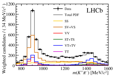
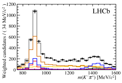
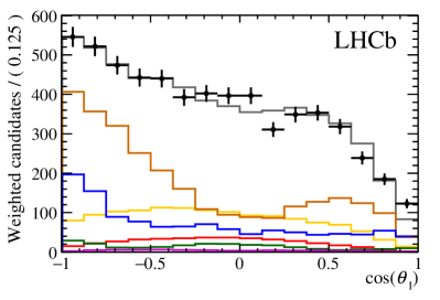
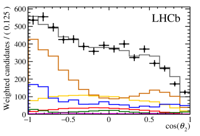
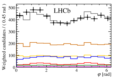
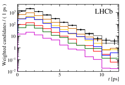
Figure 7: One-dimensional projections of the decay-time-dependent, flavour-tagged fit to (black points) the sPlot weighted data for (top row) the two $(K\pi)$ invariant masses, (middle row) the two $(K\pi)$ decay plane angles, (bottom left) the angle between the two $(K,\pi)$ decay planes and (bottom right) the decay-time. The solid gray line represents the total fit model along with the $C\!P$-averaged components for each contributing decay.

Table 5: Results of the decay-time-dependent amplitude fit to data. The first uncertainty is statistical and the second uncertainty is systematic.

Parameter	Value
Common parameters
$\phi_{s}^{{d}{\overline{d}}}$ [rad]	$-0.10\phantom{0}\pm 0.13\phantom{0}\pm 0.14\phantom{0}$
$|\lambda|$	$\phantom{-}1.035\pm 0.034\pm 0.089$
Vector/Vector (VV)
$f^{VV}$	$\phantom{-}0.067\pm 0.004\pm 0.024$
$f_{\rm L}^{VV}$	$\phantom{-}0.208\pm 0.032\pm 0.046$
$f_{\parallel}^{VV}$	$\phantom{-}0.297\pm 0.029\pm 0.042$
$\delta^{VV}_{\parallel}$ [rad]	$\phantom{-}2.40\phantom{0}\pm 0.11\phantom{0}\pm 0.33\phantom{0}$
$\delta^{VV}_{\perp}$ [rad]	$\phantom{-}2.62\phantom{0}\pm 0.26\phantom{0}\pm 0.64\phantom{0}$
Scalar/Vector (SV and VS)
$f^{SV}$	$\phantom{-}0.329\pm 0.015\pm 0.071$
$f^{VS}$	$\phantom{-}0.133\pm 0.013\pm 0.065$
$\delta^{SV}$ [rad]	$-1.31\phantom{0}\pm 0.10\phantom{0}\pm 0.35\phantom{0}$
$\delta^{VS}$ [rad]	$\phantom{-}1.86\phantom{0}\pm 0.11\phantom{0}\pm 0.41\phantom{0}$
Scalar/Scalar (SS)
$f^{SS}$	$\phantom{-}0.225\pm 0.010\pm 0.069$
$\delta^{SS}$ [rad]	$\phantom{-}1.07\phantom{0}\pm 0.10\phantom{0}\pm 0.40\phantom{0}$
Scalar/Tensor (ST and TS)
$f^{ST}$	$\phantom{-}0.014\pm 0.006\pm 0.031$
$f^{TS}$	$\phantom{-}0.025\pm 0.007\pm 0.033$
$\delta^{ST}$ [rad]	$-2.3\phantom{00}\pm 0.4\phantom{00}\pm 1.7\phantom{00}$
$\delta^{TS}$ [rad]	$-0.10\phantom{0}\pm 0.26\phantom{0}\pm 0.82\phantom{0}$

Parameter	Value
Vector/Tensor (VT and TV)
$f^{VT}$	$\phantom{-}0.160\pm 0.016\pm 0.049$
$f_{\rm L}^{VT}$	$\phantom{-}0.911\pm 0.020\pm 0.165$
$f_{\parallel}^{VT}$	$\phantom{-}0.012\pm 0.008\pm 0.053$
$f^{TV}$	$\phantom{-}0.036\pm 0.014\pm 0.048$
$f_{\rm L}^{TV}$	$\phantom{-}0.62\phantom{0}\pm 0.16\phantom{0}\pm 0.25\phantom{0}$
$f_{\parallel}^{TV}$	$\phantom{-}0.24\phantom{0}\pm 0.10\phantom{0}\pm 0.14\phantom{0}$
$\delta^{VT}_{0}$ [rad]	$-2.06\phantom{0}\pm 0.19\phantom{0}\pm 1.17\phantom{0}$
$\delta^{VT}_{\parallel}$ [rad]	$-1.8\phantom{00}\pm 0.4\phantom{00}\pm 1.0\phantom{00}$
$\delta^{VT}_{\perp}$ [rad]	$-3.2\phantom{00}\pm 0.3\phantom{00}\pm 1.2\phantom{00}$
$\delta^{TV}_{0}$ [rad]	$\phantom{-}1.91\phantom{0}\pm 0.30\phantom{0}\pm 0.80\phantom{0}$
$\delta^{TV}_{\parallel}$ [rad]	$\phantom{-}1.09\phantom{0}\pm 0.19\phantom{0}\pm 0.55\phantom{0}$
$\delta^{TV}_{\perp}$ [rad]	$\phantom{-}0.2\phantom{00}\pm 0.4\phantom{00}\pm 1.1\phantom{00}$
Tensor/Tensor (TT)
$f^{TT}$	$\phantom{-}0.011\pm 0.003\pm 0.007$
$f_{\rm L}^{TT}$	$\phantom{-}0.25\phantom{0}\pm 0.14\phantom{0}\pm 0.18\phantom{0}$
$f_{\parallel_{1}}^{TT}$	$\phantom{-}0.17\phantom{0}\pm 0.11\phantom{0}\pm 0.14\phantom{0}$
$f_{\perp_{1}}^{TT}$	$\phantom{-}0.30\phantom{0}\pm 0.18\phantom{0}\pm 0.21\phantom{0}$
$f_{\parallel_{2}}^{TT}$	$\phantom{-}0.015\pm 0.033\pm 0.107$
$\delta^{TT}_{0}$ [rad]	$\phantom{-}1.3\phantom{00}\pm 0.5\phantom{00}\pm 1.8\phantom{00}$
$\delta^{TT}_{\parallel_{1}}$ [rad]	$\phantom{-}3.00\phantom{0}\pm 0.29\phantom{0}\pm 0.57\phantom{0}$
$\delta^{TT}_{\perp_{1}}$ [rad]	$\phantom{-}2.6\phantom{00}\pm 0.4\phantom{00}\pm 1.5\phantom{00}$
$\delta^{TT}_{\parallel_{2}}$ [rad]	$\phantom{-}2.3\phantom{00}\pm 0.8\phantom{00}\pm 1.7\phantom{00}$
$\delta^{TT}_{\perp_{2}}$ [rad]	$\phantom{-}0.7\phantom{00}\pm 0.6\phantom{00}\pm 1.3\phantom{00}$

10 Summary

A flavour-tagged decay-time-dependent amplitude analysis of the ${{B}^{0}_{s}}\rightarrow({{K}^{+}}{{\pi}^{-}})({{K}^{-}}{{\pi}^{+}})$ decay, for $({{K}^{\pm}}{{\pi}^{\mp}})$ invariant masses in the range from 750 to 1600${\mathrm{\,Me\kern-1.00006ptV\!/}c^{2}}$, is performed on a data set corresponding to an integrated luminosity of $3.0\mbox{\,fb}^{-1}$ obtained by the LHCb experiment with $pp$ collisions at $\sqrt{s}=7\mathrm{\,Te\kern-1.00006ptV}$ and $\sqrt{s}=8\mathrm{\,Te\kern-1.00006ptV}$. Several quasi-two-body decay components are considered, corresponding to $({{K}^{\pm}}{{\pi}^{\mp}})$ combinations with spins of 0, 1 and 2. The longitudinal polarisation fraction for the ${{{B}^{0}_{s}}\rightarrow{{K}^{*0}}{{\kern 1.99997pt\overline{\kern-1.99997ptK}{}}{}^{*0}}}$ vector-vector decay is determined to be $f_{\rm L}^{VV}=0.208\pm 0.032\pm 0.046$, where the first uncertainty is statistical and the second one systematic. This confirms, with improved precision, the relatively low value reported previously by LHCb [14]. The first determination of the $C\!P$ asymmetry of the $(K^{+}\pi^{-})(K^{-}\pi^{+})$ final state and the best, sometimes the first, measurements of 19 $C\!P$-averaged amplitude parameters corresponding to scalar, vector and tensor final states, are also reported. This analysis determines for the first time the mixing-induced $C\!P$-violating phase $\phi_{s}$ using a ${b}\rightarrow{d}{\overline{d}}{s}$ transition. The value of this phase is measured to be $\phi_{s}^{{d}{\overline{d}}}=-0.10\pm 0.13\pm 0.14\mathrm{\,rad}$, which is consistent with both the SM expectation [7] and the corresponding LHCb result of $\phi_{s}^{{s}{\overline{s}}}=-0.17\pm 0.15\pm 0.03\mathrm{\,rad}$ measured using ${{B}^{0}_{s}}\rightarrow\phi\phi$ decays [12]. The statistical uncertainty of the two measurements is at a similar level although the systematic uncertainty of this measurement is larger, which is mainly due to the treatment of the multi-dimensional acceptance. It is expected that this can be reduced by increasing the size of the simulation sample used to determine the acceptance effects. Most other sources of systematic uncertainty are expected to scale with larger data samples.

Appendix A Angular distributions

The angular dependence of the decay amplitudes introduced in Eq. (4) is shown in Table 6.

Table 6: Functions containing the angular dependence of the amplitudes, as introduced in Eq. (4). For a discussion on some of the angular terms see Ref. [7].

$j_{1}$	$j_{2}$	$h$	$Y_{\ell_{1}}^{m_{1}}(\theta_{1},-\varphi)Y_{\ell_{2}}^{m_{2}}(\pi-\theta_{2},0)$	$\Theta^{j_{1}j_{2}}_{h}(\cos\theta_{1},\cos\theta_{2},\varphi)$
0	0	${0}$	$\sqrt{\pi}Y_{0}^{0}Y_{0}^{0}$	$\frac{1}{2\sqrt{2\pi}}$
0	1	${0}$	$\sqrt{\pi}Y_{0}^{0}Y_{1}^{0}$	$-\frac{\sqrt{3}}{2\sqrt{2\pi}}\cos\theta_{2}$
1	0	${0}$	$\sqrt{\pi}Y_{1}^{0}Y_{0}^{0}$	$\frac{\sqrt{3}}{2\sqrt{2\pi}}\cos\theta_{1}$
0	2	${0}$	$\sqrt{\pi}Y_{0}^{0}Y_{2}^{0}$	$\frac{\sqrt{5}}{4\sqrt{2\pi}}(3\cos^{2}\theta_{2}-1)$
2	0	${0}$	$\sqrt{\pi}Y_{2}^{0}Y_{0}^{0}$	$\frac{\sqrt{5}}{4\sqrt{2\pi}}(3\cos^{2}\theta_{1}-1)$
1	1	${0}$	$\sqrt{\pi}Y_{1}^{0}Y_{1}^{0}$	$-\frac{3}{2\sqrt{2\pi}}\cos\theta_{1}\cos\theta_{2}$
1	1	${\parallel}$	$\frac{\sqrt{\pi}}{\sqrt{2}}(Y_{1}^{-1}Y_{1}^{+1}+Y_{1}^{+1}Y_{1}^{-1})$	$-\frac{3}{4\sqrt{\pi}}\sin\theta_{1}\sin\theta_{2}\cos\varphi$
1	1	${\perp}$	$\frac{\sqrt{\pi}}{\sqrt{2}}(Y_{1}^{-1}Y_{1}^{+1}-Y_{1}^{+1}Y_{1}^{-1})$	$-i\frac{3}{4\sqrt{\pi}}\sin\theta_{1}\sin\theta_{2}\sin\varphi$
1	2	${0}$	$\sqrt{\pi}Y_{1}^{0}Y_{2}^{0}$	$\frac{\sqrt{15}}{4\sqrt{2\pi}}\cos\theta_{1}(3\cos^{2}\theta_{2}-1)$
1	2	${\parallel}$	$\frac{\sqrt{\pi}}{\sqrt{2}}(Y_{1}^{-1}Y_{2}^{+1}+Y_{1}^{+1}Y_{2}^{-1})$	$\frac{3\sqrt{5}}{4\sqrt{\pi}}\sin\theta_{1}\sin\theta_{2}\cos\theta_{2}\cos\varphi$
1	2	${\perp}$	$\frac{\sqrt{\pi}}{\sqrt{2}}(Y_{1}^{-1}Y_{2}^{+1}-Y_{1}^{+1}Y_{2}^{-1})$	$i\frac{3\sqrt{5}}{4\sqrt{\pi}}\sin\theta_{1}\sin\theta_{2}\cos\theta_{2}\sin\varphi$
2	1	${0}$	$\sqrt{\pi}Y_{2}^{0}Y_{1}^{0}$	$-\frac{\sqrt{15}}{4\sqrt{2\pi}}(3\cos^{2}\theta_{1}-1)\cos\theta_{2}$
2	1	${\parallel}$	$\frac{\sqrt{\pi}}{\sqrt{2}}(Y_{2}^{-1}Y_{1}^{+1}+Y_{2}^{+1}Y_{1}^{-1})$	$-\frac{3\sqrt{5}}{4\sqrt{\pi}}\sin\theta_{1}\cos\theta_{1}\sin\theta_{2}\cos\varphi$
2	1	${\perp}$	$\frac{\sqrt{\pi}}{\sqrt{2}}(Y_{2}^{-1}Y_{1}^{+1}-Y_{2}^{+1}Y_{1}^{-1})$	$-i\frac{3\sqrt{5}}{4\sqrt{\pi}}\sin\theta_{1}\cos\theta_{1}\sin\theta_{2}\sin\varphi$
2	2	${0}$	$\sqrt{\pi}Y_{2}^{0}Y_{2}^{0}$	$\frac{5}{8\sqrt{2\pi}}(3\cos^{2}\theta_{1}-1)(3\cos^{2}\theta_{2}-1)$
2	2	${\parallel_{1}}$	$\frac{\sqrt{\pi}}{\sqrt{2}}(Y_{2}^{-1}Y_{2}^{+1}+Y_{2}^{+1}Y_{2}^{-1})$	$\frac{15}{4\sqrt{\pi}}\sin\theta_{1}\cos\theta_{1}\sin\theta_{2}\cos\theta_{2}\cos\varphi$
2	2	${\perp_{1}}$	$\frac{\sqrt{\pi}}{\sqrt{2}}(Y_{2}^{-1}Y_{2}^{+1}-Y_{2}^{+1}Y_{2}^{-1})$	$i\frac{15}{4\sqrt{\pi}}\sin\theta_{1}\cos\theta_{1}\sin\theta_{2}\cos\theta_{2}\sin\varphi$
2	2	${\parallel_{2}}$	$\frac{\sqrt{\pi}}{\sqrt{2}}(Y_{2}^{-2}Y_{2}^{+2}+Y_{2}^{+2}Y_{2}^{-2})$	$\frac{15}{16\sqrt{\pi}}\sin^{2}\theta_{1}\sin^{2}\theta_{2}\cos(2\varphi)$
2	2	${\perp_{2}}$	$\frac{\sqrt{\pi}}{\sqrt{2}}(Y_{2}^{-2}Y_{2}^{+2}-Y_{2}^{+2}Y_{2}^{-2})$	$i\frac{15}{16\sqrt{\pi}}\sin^{2}\theta_{1}\sin^{2}\theta_{2}\sin(2\varphi)$

Appendix B Scalar $K\pi$ mass-dependent amplitude

The variation of the phase with $m(K\pi)$ in the nominal model used for the scalar $K\pi$ mass-dependent amplitude is taken from Ref. [17]. The modulus line-shape is parameterised with a polynomial expansion as follows

$$|\mathcal{M}_{0}(m)|=1+\sum_{i=1}^{4}c_{i}\,T_{i}(X(m)),$$ (20)

where $X(m)=(m-1175\,{\rm MeV}/c^{2})/425\,{\rm MeV}/c^{2}$ $X(m)\in[-1,1]$, and $T_{i}(x)$ are the Chebyshev polynomials defined as

$$T_{0}(x)=1$$, , ,

, .

(21)

This parameterisation is chosen to minimise parameter correlations. The values of the $c_{i}$ coefficients retrieved from the decay-time-dependent fit are given in Table 7. The coefficients decrease with the order of the polynomial term. The expansion is truncated at fourth order since adding an extra term would not significantly affect the result and the size of the fifth coefficient is of the order of its statistical uncertainty.

Table 7: Parameters used in the nominal model for the scalar $K\pi$ mass-dependent amplitude. The correlations among them are found to be small, the largest ones been of the order of $50\%$.

Parameter	Value
$c_{1}$	$-0.287\pm 0.020$
$c_{2}$	$-0.180\pm 0.020$
$c_{3}$	$-0.106\pm 0.016$
$c_{4}$	$-0.066\pm 0.016$

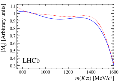
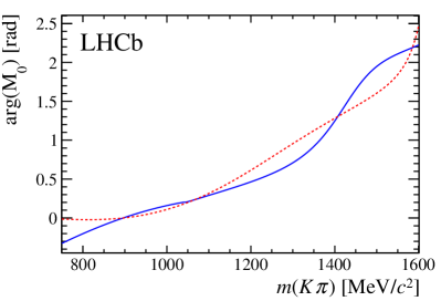
Figure 8: Line-shapes of the (left) modulus and (right) phase of the scalar $K\pi$ mass-dependent amplitude. The nominal model is shown with a solid blue line and the model-independent parameterisation, used in systematic studies, is shown with a dashed red line.

When computing systematic uncertainties, the scalar $K\pi$ mass-dependent amplitude is parameterised using a model-independent (MI) approach as follows

$$\mathcal{M}_{0}^{MI}(m)=\left[1+\sum_{i=1}^{4}\alpha_{i}\,T_{i}(X(m))\right]+i\,\left[\sum_{j=0}^{4}\beta_{j}\,T_{j}(X(m))\right].$$ (22)

The coefficients measured in the decay-time-dependent fit for this case are given in Table 8.

Table 8: Coefficients used in the model-independent parameterisation of the scalar $K\pi$ mass-dependent amplitude.

Parameter	Value	Parameter	Value
$\alpha_{1}$	$-0.854\pm 0.038$	$\beta_{0}$	$\phantom{-}0.278\pm 0.038$
$\alpha_{2}$	$-0.381\pm 0.040$	$\beta_{1}$	$\phantom{-}0.817\pm 0.079$
$\alpha_{3}$	$-0.105\pm 0.032$	$\beta_{2}$	$-0.206\pm 0.082$
$\alpha_{4}$	$\phantom{-}0.046\pm 0.027$	$\beta_{3}$	$-0.367\pm 0.053$
		$\beta_{4}$	$-0.115\pm 0.040$

The line-shapes of the two scalar mass amplitude models are shown in Fig. 8. Both approaches are found to be qualitatively compatible with each other.

LHCb collaboration

R. Aaij⁴⁰, B. Adeva³⁹, M. Adinolfi⁴⁸, Z. Ajaltouni⁵, S. Akar⁵⁹, J. Albrecht¹⁰, F. Alessio⁴⁰, M. Alexander⁵³, A. Alfonso Albero³⁸, S. Ali⁴³, G. Alkhazov³¹, P. Alvarez Cartelle⁵⁵, A.A. Alves Jr⁵⁹, S. Amato², S. Amerio²³, Y. Amhis⁷, L. An³, L. Anderlini¹⁸, G. Andreassi⁴¹, M. Andreotti^17,g, J.E. Andrews⁶⁰, R.B. Appleby⁵⁶, F. Archilli⁴³, P. d’Argent¹², J. Arnau Romeu⁶, A. Artamonov³⁷, M. Artuso⁶¹, E. Aslanides⁶, M. Atzeni⁴², G. Auriemma²⁶, M. Baalouch⁵, I. Babuschkin⁵⁶, S. Bachmann¹², J.J. Back⁵⁰, A. Badalov^38,m, C. Baesso⁶², S. Baker⁵⁵, V. Balagura^7,b, W. Baldini¹⁷, A. Baranov³⁵, R.J. Barlow⁵⁶, C. Barschel⁴⁰, S. Barsuk⁷, W. Barter⁵⁶, F. Baryshnikov³², V. Batozskaya²⁹, V. Battista⁴¹, A. Bay⁴¹, L. Beaucourt⁴, J. Beddow⁵³, F. Bedeschi²⁴, I. Bediaga¹, A. Beiter⁶¹, L.J. Bel⁴³, N. Beliy⁶³, V. Bellee⁴¹, N. Belloli^21,i, K. Belous³⁷, I. Belyaev^32,40, E. Ben-Haim⁸, G. Bencivenni¹⁹, S. Benson⁴³, S. Beranek⁹, A. Berezhnoy³³, R. Bernet⁴², D. Berninghoff¹², E. Bertholet⁸, A. Bertolin²³, C. Betancourt⁴², F. Betti¹⁵, M.O. Bettler⁴⁰, M. van Beuzekom⁴³, Ia. Bezshyiko⁴², S. Bifani⁴⁷, P. Billoir⁸, A. Birnkraut¹⁰, A. Bizzeti^18,u, M. Bjørn⁵⁷, T. Blake⁵⁰, F. Blanc⁴¹, S. Blusk⁶¹, V. Bocci²⁶, T. Boettcher⁵⁸, A. Bondar^36,w, N. Bondar³¹, I. Bordyuzhin³², S. Borghi^56,40, M. Borisyak³⁵, M. Borsato³⁹, F. Bossu⁷, M. Boubdir⁹, T.J.V. Bowcock⁵⁴, E. Bowen⁴², C. Bozzi^17,40, S. Braun¹², J. Brodzicka²⁷, D. Brundu¹⁶, E. Buchanan⁴⁸, C. Burr⁵⁶, A. Bursche^16,f, J. Buytaert⁴⁰, W. Byczynski⁴⁰, S. Cadeddu¹⁶, H. Cai⁶⁴, R. Calabrese^17,g, R. Calladine⁴⁷, M. Calvi^21,i, M. Calvo Gomez^38,m, A. Camboni^38,m, P. Campana¹⁹, D.H. Campora Perez⁴⁰, L. Capriotti⁵⁶, A. Carbone^15,e, G. Carboni^25,j, R. Cardinale^20,h, A. Cardini¹⁶, P. Carniti^21,i, L. Carson⁵², K. Carvalho Akiba², G. Casse⁵⁴, L. Cassina²¹, M. Cattaneo⁴⁰, G. Cavallero^20,40,h, R. Cenci^24,t, D. Chamont⁷, M.G. Chapman⁴⁸, M. Charles⁸, Ph. Charpentier⁴⁰, G. Chatzikonstantinidis⁴⁷, M. Chefdeville⁴, S. Chen¹⁶, S.F. Cheung⁵⁷, S.-G. Chitic⁴⁰, V. Chobanova³⁹, M. Chrzaszcz⁴², A. Chubykin³¹, P. Ciambrone¹⁹, X. Cid Vidal³⁹, G. Ciezarek⁴⁰, P.E.L. Clarke⁵², M. Clemencic⁴⁰, H.V. Cliff⁴⁹, J. Closier⁴⁰, V. Coco⁴⁰, J. Cogan⁶, E. Cogneras⁵, V. Cogoni^16,f, L. Cojocariu³⁰, P. Collins⁴⁰, T. Colombo⁴⁰, A. Comerma-Montells¹², A. Contu¹⁶, G. Coombs⁴⁰, S. Coquereau³⁸, G. Corti⁴⁰, M. Corvo^17,g, C.M. Costa Sobral⁵⁰, B. Couturier⁴⁰, G.A. Cowan⁵², D.C. Craik⁵⁸, A. Crocombe⁵⁰, M. Cruz Torres¹, R. Currie⁵², C. D’Ambrosio⁴⁰, F. Da Cunha Marinho², C.L. Da Silva⁷³, E. Dall’Occo⁴³, J. Dalseno⁴⁸, A. Davis³, O. De Aguiar Francisco⁴⁰, K. De Bruyn⁴⁰, S. De Capua⁵⁶, M. De Cian¹², J.M. De Miranda¹, L. De Paula², M. De Serio^14,d, P. De Simone¹⁹, C.T. Dean⁵³, D. Decamp⁴, L. Del Buono⁸, H.-P. Dembinski¹¹, M. Demmer¹⁰, A. Dendek²⁸, D. Derkach³⁵, O. Deschamps⁵, F. Dettori⁵⁴, B. Dey⁶⁵, A. Di Canto⁴⁰, P. Di Nezza¹⁹, H. Dijkstra⁴⁰, F. Dordei⁴⁰, M. Dorigo⁴⁰, A. Dosil Suárez³⁹, L. Douglas⁵³, A. Dovbnya⁴⁵, K. Dreimanis⁵⁴, L. Dufour⁴³, G. Dujany⁸, P. Durante⁴⁰, J.M. Durham⁷³, D. Dutta⁵⁶, R. Dzhelyadin³⁷, M. Dziewiecki¹², A. Dziurda⁴⁰, A. Dzyuba³¹, S. Easo⁵¹, U. Egede⁵⁵, V. Egorychev³², S. Eidelman^36,w, S. Eisenhardt⁵², U. Eitschberger¹⁰, R. Ekelhof¹⁰, L. Eklund⁵³, S. Ely⁶¹, S. Esen¹², H.M. Evans⁴⁹, T. Evans⁵⁷, A. Falabella¹⁵, N. Farley⁴⁷, S. Farry⁵⁴, D. Fazzini^21,i, L. Federici²⁵, D. Ferguson⁵², G. Fernandez³⁸, P. Fernandez Declara⁴⁰, A. Fernandez Prieto³⁹, F. Ferrari¹⁵, L. Ferreira Lopes⁴¹, F. Ferreira Rodrigues², M. Ferro-Luzzi⁴⁰, S. Filippov³⁴, R.A. Fini¹⁴, M. Fiorini^17,g, M. Firlej²⁸, C. Fitzpatrick⁴¹, T. Fiutowski²⁸, F. Fleuret^7,b, M. Fontana^16,40, F. Fontanelli^20,h, R. Forty⁴⁰, V. Franco Lima⁵⁴, M. Frank⁴⁰, C. Frei⁴⁰, J. Fu^22,q, W. Funk⁴⁰, E. Furfaro^25,j, C. Färber⁴⁰, E. Gabriel⁵², A. Gallas Torreira³⁹, D. Galli^15,e, S. Gallorini²³, S. Gambetta⁵², M. Gandelman², P. Gandini²², Y. Gao³, L.M. Garcia Martin⁷¹, J. García Pardiñas³⁹, J. Garra Tico⁴⁹, L. Garrido³⁸, D. Gascon³⁸, C. Gaspar⁴⁰, L. Gavardi¹⁰, G. Gazzoni⁵, D. Gerick¹², E. Gersabeck⁵⁶, M. Gersabeck⁵⁶, T. Gershon⁵⁰, Ph. Ghez⁴, S. Gianì⁴¹, V. Gibson⁴⁹, O.G. Girard⁴¹, L. Giubega³⁰, K. Gizdov⁵², V.V. Gligorov⁸, D. Golubkov³², A. Golutvin^55,69, A. Gomes^1,a, I.V. Gorelov³³, C. Gotti^21,i, E. Govorkova⁴³, J.P. Grabowski¹², R. Graciani Diaz³⁸, L.A. Granado Cardoso⁴⁰, E. Graugés³⁸, E. Graverini⁴², G. Graziani¹⁸, A. Grecu³⁰, R. Greim⁹, P. Griffith¹⁶, L. Grillo⁵⁶, L. Gruber⁴⁰, B.R. Gruberg Cazon⁵⁷, O. Grünberg⁶⁷, E. Gushchin³⁴, Yu. Guz³⁷, T. Gys⁴⁰, C. Göbel⁶², T. Hadavizadeh⁵⁷, C. Hadjivasiliou⁵, G. Haefeli⁴¹, C. Haen⁴⁰, S.C. Haines⁴⁹, B. Hamilton⁶⁰, X. Han¹², T.H. Hancock⁵⁷, S. Hansmann-Menzemer¹², N. Harnew⁵⁷, S.T. Harnew⁴⁸, C. Hasse⁴⁰, M. Hatch⁴⁰, J. He⁶³, M. Hecker⁵⁵, K. Heinicke¹⁰, A. Heister⁹, K. Hennessy⁵⁴, P. Henrard⁵, L. Henry⁷¹, E. van Herwijnen⁴⁰, M. Heß⁶⁷, A. Hicheur², D. Hill⁵⁷, P.H. Hopchev⁴¹, W. Hu⁶⁵, W. Huang⁶³, Z.C. Huard⁵⁹, W. Hulsbergen⁴³, T. Humair⁵⁵, M. Hushchyn³⁵, D. Hutchcroft⁵⁴, P. Ibis¹⁰, M. Idzik²⁸, P. Ilten⁴⁷, R. Jacobsson⁴⁰, J. Jalocha⁵⁷, E. Jans⁴³, A. Jawahery⁶⁰, F. Jiang³, M. John⁵⁷, D. Johnson⁴⁰, C.R. Jones⁴⁹, C. Joram⁴⁰, B. Jost⁴⁰, N. Jurik⁵⁷, S. Kandybei⁴⁵, M. Karacson⁴⁰, J.M. Kariuki⁴⁸, S. Karodia⁵³, N. Kazeev³⁵, M. Kecke¹², F. Keizer⁴⁹, M. Kelsey⁶¹, M. Kenzie⁴⁹, T. Ketel⁴⁴, E. Khairullin³⁵, B. Khanji¹², C. Khurewathanakul⁴¹, K.E. Kim⁶¹, T. Kirn⁹, S. Klaver¹⁹, K. Klimaszewski²⁹, T. Klimkovich¹¹, S. Koliiev⁴⁶, M. Kolpin¹², R. Kopecna¹², P. Koppenburg⁴³, A. Kosmyntseva³², S. Kotriakhova³¹, M. Kozeiha⁵, L. Kravchuk³⁴, M. Kreps⁵⁰, F. Kress⁵⁵, P. Krokovny^36,w, W. Krzemien²⁹, W. Kucewicz^27,l, M. Kucharczyk²⁷, V. Kudryavtsev^36,w, A.K. Kuonen⁴¹, T. Kvaratskheliya^32,40, D. Lacarrere⁴⁰, G. Lafferty⁵⁶, A. Lai¹⁶, G. Lanfranchi¹⁹, C. Langenbruch⁹, T. Latham⁵⁰, C. Lazzeroni⁴⁷, R. Le Gac⁶, A. Leflat^33,40, J. Lefrançois⁷, R. Lefèvre⁵, F. Lemaitre⁴⁰, E. Lemos Cid³⁹, O. Leroy⁶, T. Lesiak²⁷, B. Leverington¹², P.-R. Li⁶³, T. Li³, Y. Li⁷, Z. Li⁶¹, X. Liang⁶¹, T. Likhomanenko⁶⁸, R. Lindner⁴⁰, F. Lionetto⁴², V. Lisovskyi⁷, X. Liu³, D. Loh⁵⁰, A. Loi¹⁶, I. Longstaff⁵³, J.H. Lopes², D. Lucchesi^23,o, M. Lucio Martinez³⁹, H. Luo⁵², A. Lupato²³, E. Luppi^17,g, O. Lupton⁴⁰, A. Lusiani²⁴, X. Lyu⁶³, F. Machefert⁷, F. Maciuc³⁰, V. Macko⁴¹, P. Mackowiak¹⁰, S. Maddrell-Mander⁴⁸, O. Maev^31,40, K. Maguire⁵⁶, D. Maisuzenko³¹, M.W. Majewski²⁸, S. Malde⁵⁷, B. Malecki²⁷, A. Malinin⁶⁸, T. Maltsev^36,w, G. Manca^16,f, G. Mancinelli⁶, D. Marangotto^22,q, J. Maratas^5,v, J.F. Marchand⁴, U. Marconi¹⁵, C. Marin Benito³⁸, M. Marinangeli⁴¹, P. Marino⁴¹, J. Marks¹², G. Martellotti²⁶, M. Martin⁶, M. Martinelli⁴¹, D. Martinez Santos³⁹, F. Martinez Vidal⁷¹, A. Massafferri¹, R. Matev⁴⁰, A. Mathad⁵⁰, Z. Mathe⁴⁰, C. Matteuzzi²¹, A. Mauri⁴², E. Maurice^7,b, B. Maurin⁴¹, A. Mazurov⁴⁷, M. McCann^55,40, A. McNab⁵⁶, R. McNulty¹³, J.V. Mead⁵⁴, B. Meadows⁵⁹, C. Meaux⁶, F. Meier¹⁰, N. Meinert⁶⁷, D. Melnychuk²⁹, M. Merk⁴³, A. Merli^22,40,q, E. Michielin²³, D.A. Milanes⁶⁶, E. Millard⁵⁰, M.-N. Minard⁴, L. Minzoni¹⁷, D.S. Mitzel¹², A. Mogini⁸, J. Molina Rodriguez¹, T. Mombächer¹⁰, I.A. Monroy⁶⁶, S. Monteil⁵, M. Morandin²³, M.J. Morello^24,t, O. Morgunova⁶⁸, J. Moron²⁸, A.B. Morris⁵², R. Mountain⁶¹, F. Muheim⁵², M. Mulder⁴³, D. Müller⁵⁶, J. Müller¹⁰, K. Müller⁴², V. Müller¹⁰, P. Naik⁴⁸, T. Nakada⁴¹, R. Nandakumar⁵¹, A. Nandi⁵⁷, I. Nasteva², M. Needham⁵², N. Neri^22,40, S. Neubert¹², N. Neufeld⁴⁰, M. Neuner¹², T.D. Nguyen⁴¹, C. Nguyen-Mau^41,n, S. Nieswand⁹, R. Niet¹⁰, N. Nikitin³³, T. Nikodem¹², A. Nogay⁶⁸, D.P. O’Hanlon⁵⁰, A. Oblakowska-Mucha²⁸, V. Obraztsov³⁷, S. Ogilvy¹⁹, R. Oldeman^16,f, C.J.G. Onderwater⁷², A. Ossowska²⁷, J.M. Otalora Goicochea², P. Owen⁴², A. Oyanguren⁷¹, P.R. Pais⁴¹, A. Palano¹⁴, M. Palutan^19,40, G. Panshin⁷⁰, A. Papanestis⁵¹, M. Pappagallo⁵², L.L. Pappalardo^17,g, W. Parker⁶⁰, C. Parkes⁵⁶, G. Passaleva^18,40, A. Pastore^14,d, M. Patel⁵⁵, C. Patrignani^15,e, A. Pearce⁴⁰, A. Pellegrino⁴³, G. Penso²⁶, M. Pepe Altarelli⁴⁰, S. Perazzini⁴⁰, D. Pereima³², P. Perret⁵, L. Pescatore⁴¹, K. Petridis⁴⁸, A. Petrolini^20,h, A. Petrov⁶⁸, M. Petruzzo^22,q, E. Picatoste Olloqui³⁸, B. Pietrzyk⁴, G. Pietrzyk⁴¹, M. Pikies²⁷, D. Pinci²⁶, F. Pisani⁴⁰, A. Pistone^20,h, A. Piucci¹², V. Placinta³⁰, S. Playfer⁵², M. Plo Casasus³⁹, F. Polci⁸, M. Poli Lener¹⁹, A. Poluektov⁵⁰, I. Polyakov⁶¹, E. Polycarpo², G.J. Pomery⁴⁸, S. Ponce⁴⁰, A. Popov³⁷, D. Popov^11,40, S. Poslavskii³⁷, C. Potterat², E. Price⁴⁸, J. Prisciandaro³⁹, C. Prouve⁴⁸, V. Pugatch⁴⁶, A. Puig Navarro⁴², H. Pullen⁵⁷, G. Punzi^24,p, W. Qian⁵⁰, J. Qin⁶³, R. Quagliani⁸, B. Quintana⁵, B. Rachwal²⁸, J.H. Rademacker⁴⁸, M. Rama²⁴, M. Ramos Pernas³⁹, M.S. Rangel², I. Raniuk^45,†, F. Ratnikov^35,x, G. Raven⁴⁴, M. Ravonel Salzgeber⁴⁰, M. Reboud⁴, F. Redi⁴¹, S. Reichert¹⁰, A.C. dos Reis¹, C. Remon Alepuz⁷¹, V. Renaudin⁷, S. Ricciardi⁵¹, S. Richards⁴⁸, M. Rihl⁴⁰, K. Rinnert⁵⁴, P. Robbe⁷, A. Robert⁸, A.B. Rodrigues⁴¹, E. Rodrigues⁵⁹, J.A. Rodriguez Lopez⁶⁶, A. Rogozhnikov³⁵, S. Roiser⁴⁰, A. Rollings⁵⁷, V. Romanovskiy³⁷, A. Romero Vidal^39,40, M. Rotondo¹⁹, M.S. Rudolph⁶¹, T. Ruf⁴⁰, P. Ruiz Valls⁷¹, J. Ruiz Vidal⁷¹, J.J. Saborido Silva³⁹, E. Sadykhov³², N. Sagidova³¹, B. Saitta^16,f, V. Salustino Guimaraes⁶², C. Sanchez Mayordomo⁷¹, B. Sanmartin Sedes³⁹, R. Santacesaria²⁶, C. Santamarina Rios³⁹, M. Santimaria¹⁹, E. Santovetti^25,j, G. Sarpis⁵⁶, A. Sarti^19,k, C. Satriano^26,s, A. Satta²⁵, D.M. Saunders⁴⁸, D. Savrina^32,33, S. Schael⁹, M. Schellenberg¹⁰, M. Schiller⁵³, H. Schindler⁴⁰, M. Schmelling¹¹, T. Schmelzer¹⁰, B. Schmidt⁴⁰, O. Schneider⁴¹, A. Schopper⁴⁰, H.F. Schreiner⁵⁹, M. Schubiger⁴¹, M.H. Schune⁷, R. Schwemmer⁴⁰, B. Sciascia¹⁹, A. Sciubba^26,k, A. Semennikov³², E.S. Sepulveda⁸, A. Sergi⁴⁷, N. Serra⁴², J. Serrano⁶, L. Sestini²³, P. Seyfert⁴⁰, M. Shapkin³⁷, I. Shapoval⁴⁵, Y. Shcheglov³¹, T. Shears⁵⁴, L. Shekhtman^36,w, V. Shevchenko⁶⁸, B.G. Siddi¹⁷, R. Silva Coutinho⁴², L. Silva de Oliveira², G. Simi^23,o, S. Simone^14,d, M. Sirendi⁴⁹, N. Skidmore⁴⁸, T. Skwarnicki⁶¹, I.T. Smith⁵², J. Smith⁴⁹, M. Smith⁵⁵, l. Soares Lavra¹, M.D. Sokoloff⁵⁹, F.J.P. Soler⁵³, B. Souza De Paula², B. Spaan¹⁰, P. Spradlin⁵³, S. Sridharan⁴⁰, F. Stagni⁴⁰, M. Stahl¹², S. Stahl⁴⁰, P. Stefko⁴¹, S. Stefkova⁵⁵, O. Steinkamp⁴², S. Stemmle¹², O. Stenyakin³⁷, M. Stepanova³¹, H. Stevens¹⁰, S. Stone⁶¹, B. Storaci⁴², S. Stracka^24,p, M.E. Stramaglia⁴¹, M. Straticiuc³⁰, U. Straumann⁴², S. Strokov⁷⁰, J. Sun³, L. Sun⁶⁴, K. Swientek²⁸, V. Syropoulos⁴⁴, T. Szumlak²⁸, M. Szymanski⁶³, S. T’Jampens⁴, A. Tayduganov⁶, T. Tekampe¹⁰, G. Tellarini^17,g, F. Teubert⁴⁰, E. Thomas⁴⁰, J. van Tilburg⁴³, M.J. Tilley⁵⁵, V. Tisserand⁵, M. Tobin⁴¹, S. Tolk⁴⁹, L. Tomassetti^17,g, D. Tonelli²⁴, R. Tourinho Jadallah Aoude¹, E. Tournefier⁴, M. Traill⁵³, M.T. Tran⁴¹, M. Tresch⁴², A. Trisovic⁴⁹, A. Tsaregorodtsev⁶, P. Tsopelas⁴³, A. Tully⁴⁹, N. Tuning^43,40, A. Ukleja²⁹, A. Usachov⁷, A. Ustyuzhanin³⁵, U. Uwer¹², C. Vacca^16,f, A. Vagner⁷⁰, V. Vagnoni^15,40, A. Valassi⁴⁰, S. Valat⁴⁰, G. Valenti¹⁵, R. Vazquez Gomez⁴⁰, P. Vazquez Regueiro³⁹, S. Vecchi¹⁷, M. van Veghel⁴³, J.J. Velthuis⁴⁸, M. Veltri^18,r, G. Veneziano⁵⁷, A. Venkateswaran⁶¹, T.A. Verlage⁹, M. Vernet⁵, M. Vesterinen⁵⁷, J.V. Viana Barbosa⁴⁰, D.  Vieira⁶³, M. Vieites Diaz³⁹, H. Viemann⁶⁷, X. Vilasis-Cardona^38,m, M. Vitti⁴⁹, V. Volkov³³, A. Vollhardt⁴², B. Voneki⁴⁰, A. Vorobyev³¹, V. Vorobyev^36,w, C. Voß⁹, J.A. de Vries⁴³, C. Vázquez Sierra⁴³, R. Waldi⁶⁷, J. Walsh²⁴, J. Wang⁶¹, Y. Wang⁶⁵, D.R. Ward⁴⁹, H.M. Wark⁵⁴, N.K. Watson⁴⁷, D. Websdale⁵⁵, A. Weiden⁴², C. Weisser⁵⁸, M. Whitehead⁴⁰, J. Wicht⁵⁰, G. Wilkinson⁵⁷, M. Wilkinson⁶¹, M. Williams⁵⁶, M. Williams⁵⁸, T. Williams⁴⁷, F.F. Wilson^51,40, J. Wimberley⁶⁰, M. Winn⁷, J. Wishahi¹⁰, W. Wislicki²⁹, M. Witek²⁷, G. Wormser⁷, S.A. Wotton⁴⁹, K. Wyllie⁴⁰, Y. Xie⁶⁵, M. Xu⁶⁵, Q. Xu⁶³, Z. Xu³, Z. Xu⁴, Z. Yang³, Z. Yang⁶⁰, Y. Yao⁶¹, H. Yin⁶⁵, J. Yu⁶⁵, X. Yuan⁶¹, O. Yushchenko³⁷, K.A. Zarebski⁴⁷, M. Zavertyaev^11,c, L. Zhang³, Y. Zhang⁷, A. Zhelezov¹², Y. Zheng⁶³, X. Zhu³, V. Zhukov^9,33, J.B. Zonneveld⁵², S. Zucchelli¹⁵.
¹Centro Brasileiro de Pesquisas Físicas (CBPF), Rio de Janeiro, Brazil
²Universidade Federal do Rio de Janeiro (UFRJ), Rio de Janeiro, Brazil
³Center for High Energy Physics, Tsinghua University, Beijing, China
⁴Univ. Grenoble Alpes, Univ. Savoie Mont Blanc, CNRS, IN2P3-LAPP, Annecy, France
⁵Clermont Université, Université Blaise Pascal, CNRS/IN2P3, LPC, Clermont-Ferrand, France
⁶Aix Marseille Univ, CNRS/IN2P3, CPPM, Marseille, France
⁷LAL, Univ. Paris-Sud, CNRS/IN2P3, Université Paris-Saclay, Orsay, France
⁸LPNHE, Université Pierre et Marie Curie, Université Paris Diderot, CNRS/IN2P3, Paris, France
⁹I. Physikalisches Institut, RWTH Aachen University, Aachen, Germany
¹⁰Fakultät Physik, Technische Universität Dortmund, Dortmund, Germany
¹¹Max-Planck-Institut für Kernphysik (MPIK), Heidelberg, Germany
¹²Physikalisches Institut, Ruprecht-Karls-Universität Heidelberg, Heidelberg, Germany
¹³School of Physics, University College Dublin, Dublin, Ireland
¹⁴Sezione INFN di Bari, Bari, Italy
¹⁵Sezione INFN di Bologna, Bologna, Italy
¹⁶Sezione INFN di Cagliari, Cagliari, Italy
¹⁷Universita e INFN, Ferrara, Ferrara, Italy
¹⁸Sezione INFN di Firenze, Firenze, Italy
¹⁹Laboratori Nazionali dell’INFN di Frascati, Frascati, Italy
²⁰Sezione INFN di Genova, Genova, Italy
²¹Sezione INFN di Milano Bicocca, Milano, Italy
²²Sezione di Milano, Milano, Italy
²³Sezione INFN di Padova, Padova, Italy
²⁴Sezione INFN di Pisa, Pisa, Italy
²⁵Sezione INFN di Roma Tor Vergata, Roma, Italy
²⁶Sezione INFN di Roma La Sapienza, Roma, Italy
²⁷Henryk Niewodniczanski Institute of Nuclear Physics Polish Academy of Sciences, Kraków, Poland
²⁸AGH - University of Science and Technology, Faculty of Physics and Applied Computer Science, Kraków, Poland
²⁹National Center for Nuclear Research (NCBJ), Warsaw, Poland
³⁰Horia Hulubei National Institute of Physics and Nuclear Engineering, Bucharest-Magurele, Romania
³¹Petersburg Nuclear Physics Institute (PNPI), Gatchina, Russia
³²Institute of Theoretical and Experimental Physics (ITEP), Moscow, Russia
³³Institute of Nuclear Physics, Moscow State University (SINP MSU), Moscow, Russia
³⁴Institute for Nuclear Research of the Russian Academy of Sciences (INR RAS), Moscow, Russia
³⁵Yandex School of Data Analysis, Moscow, Russia
³⁶Budker Institute of Nuclear Physics (SB RAS), Novosibirsk, Russia
³⁷Institute for High Energy Physics (IHEP), Protvino, Russia
³⁸ICCUB, Universitat de Barcelona, Barcelona, Spain
³⁹Instituto Galego de Física de Altas Enerxías (IGFAE), Universidade de Santiago de Compostela, Santiago de Compostela, Spain
⁴⁰European Organization for Nuclear Research (CERN), Geneva, Switzerland
⁴¹Institute of Physics, Ecole Polytechnique Fédérale de Lausanne (EPFL), Lausanne, Switzerland
⁴²Physik-Institut, Universität Zürich, Zürich, Switzerland
⁴³Nikhef National Institute for Subatomic Physics, Amsterdam, The Netherlands
⁴⁴Nikhef National Institute for Subatomic Physics and VU University Amsterdam, Amsterdam, The Netherlands
⁴⁵NSC Kharkiv Institute of Physics and Technology (NSC KIPT), Kharkiv, Ukraine
⁴⁶Institute for Nuclear Research of the National Academy of Sciences (KINR), Kyiv, Ukraine
⁴⁷University of Birmingham, Birmingham, United Kingdom
⁴⁸H.H. Wills Physics Laboratory, University of Bristol, Bristol, United Kingdom
⁴⁹Cavendish Laboratory, University of Cambridge, Cambridge, United Kingdom
⁵⁰Department of Physics, University of Warwick, Coventry, United Kingdom
⁵¹STFC Rutherford Appleton Laboratory, Didcot, United Kingdom
⁵²School of Physics and Astronomy, University of Edinburgh, Edinburgh, United Kingdom
⁵³School of Physics and Astronomy, University of Glasgow, Glasgow, United Kingdom
⁵⁴Oliver Lodge Laboratory, University of Liverpool, Liverpool, United Kingdom
⁵⁵Imperial College London, London, United Kingdom
⁵⁶School of Physics and Astronomy, University of Manchester, Manchester, United Kingdom
⁵⁷Department of Physics, University of Oxford, Oxford, United Kingdom
⁵⁸Massachusetts Institute of Technology, Cambridge, MA, United States
⁵⁹University of Cincinnati, Cincinnati, OH, United States
⁶⁰University of Maryland, College Park, MD, United States
⁶¹Syracuse University, Syracuse, NY, United States
⁶²Pontifícia Universidade Católica do Rio de Janeiro (PUC-Rio), Rio de Janeiro, Brazil, associated to ^2
63University of Chinese Academy of Sciences, Beijing, China, associated to ^3
64School of Physics and Technology, Wuhan University, Wuhan, China, associated to ^3
65Institute of Particle Physics, Central China Normal University, Wuhan, Hubei, China, associated to ^3
66Departamento de Fisica , Universidad Nacional de Colombia, Bogota, Colombia, associated to ^8
67Institut für Physik, Universität Rostock, Rostock, Germany, associated to ^12
68National Research Centre Kurchatov Institute, Moscow, Russia, associated to ^32
69National University of Science and Technology MISIS, Moscow, Russia, associated to ^32
70National Research Tomsk Polytechnic University, Tomsk, Russia, associated to ^32
71Instituto de Fisica Corpuscular, Centro Mixto Universidad de Valencia - CSIC, Valencia, Spain, associated to ^38
72Van Swinderen Institute, University of Groningen, Groningen, The Netherlands, associated to ^43
73Los Alamos National Laboratory (LANL), Los Alamos, United States, associated to <sup>61

a</sup>Universidade Federal do Triângulo Mineiro (UFTM), Uberaba-MG, Brazil
^bLaboratoire Leprince-Ringuet, Palaiseau, France
^cP.N. Lebedev Physical Institute, Russian Academy of Science (LPI RAS), Moscow, Russia
^dUniversità di Bari, Bari, Italy
^eUniversità di Bologna, Bologna, Italy
^fUniversità di Cagliari, Cagliari, Italy
^gUniversità di Ferrara, Ferrara, Italy
^hUniversità di Genova, Genova, Italy
ⁱUniversità di Milano Bicocca, Milano, Italy
^jUniversità di Roma Tor Vergata, Roma, Italy
^kUniversità di Roma La Sapienza, Roma, Italy
^lAGH - University of Science and Technology, Faculty of Computer Science, Electronics and Telecommunications, Kraków, Poland
^mLIFAELS, La Salle, Universitat Ramon Llull, Barcelona, Spain
ⁿHanoi University of Science, Hanoi, Vietnam
^oUniversità di Padova, Padova, Italy
^pUniversità di Pisa, Pisa, Italy
^qUniversità degli Studi di Milano, Milano, Italy
^rUniversità di Urbino, Urbino, Italy
^sUniversità della Basilicata, Potenza, Italy
^tScuola Normale Superiore, Pisa, Italy
^uUniversità di Modena e Reggio Emilia, Modena, Italy
^vIligan Institute of Technology (IIT), Iligan, Philippines
^wNovosibirsk State University, Novosibirsk, Russia
^xNational Research University Higher School of Economics, Moscow, Russia
^†Deceased

References

- [1] R. Fleischer, Extracting CKM phases from angular distributions of decays into admixtures of CP eigenstates, Phys. Rev. D60 (1999) 073008, arXiv:hep-ph/9903540
- [2] R. Fleischer and M. Gronau, Studying new physics amplitudes in charmless decays, Phys. Lett. B660 (2008) 212, arXiv:0709.4013
- [3] M. Ciuchini, M. Pierini, and L. Silvestrini, CP asymmetries: Golden channels for new physics searches, Phys. Rev. Lett. 100 (2008) 031802, arXiv:hep-ph/0703137
- [4] S. Descotes-Genon, J. Matias, and J. Virto, Penguin-mediated decays and the mixing angle, Phys. Rev. D76 (2007) 074005, Erratum ibid. D84 (2011) 039901, arXiv:0705.0477
- [5] S. Descotes-Genon, J. Matias, and J. Virto, Analysis of mixing angles in presence of new physics and an update of , Phys. Rev. D85 (2012) 034010, arXiv:1111.4882
- [6] B. Bhattacharya, A. Datta, M. Imbeault, and D. London, Searching for new physics with – a reappraisal, Phys. Lett. B717 (2012) 403, arXiv:1203.3435
- [7] B. Bhattacharya, A. Datta, M. Duraisamy, and D. London, Searching for new physics with penguin decays, Phys. Rev. D88 (2013) 016007, arXiv:1306.1911
- [8] Heavy Flavor Averaging Group, Y. Amhis et al., Averages of -hadron, -hadron, and -lepton properties as of summer 2016, arXiv:1612.07233, updated results and plots available at http://www.slac.stanford.edu/xorg/hflav/
- [9] LHCb collaboration, R. Aaij et al., Precision measurement of violation in decays, Phys. Rev. Lett. 114 (2015) 041801, arXiv:1411.3104
- [10] ATLAS collaboration, G. Aad et al., Measurement of the CP-violating phase and the meson decay width difference with decays in ATLAS, JHEP 08 (2016) 147, arXiv:1601.03297
- [11] CMS collaboration, V. Khachatryan et al., Measurement of the CP-violating weak phase and the decay width difference using the (1020) decay channel in collisions at 8 TeV, Phys. Lett. B757 (2016) 97, arXiv:1507.07527
- [12] LHCb collaboration, R. Aaij et al., Measurement of violation in decays, Phys. Rev. D90 (2014) 052011, arXiv:1407.2222
- [13] LHCb collaboration, R. Aaij et al., First observation of the decay , Phys. Lett. B709 (2012) 50, arXiv:1111.4183
- [14] LHCb collaboration, R. Aaij et al., Measurement of asymmetries and polarisation fractions in decays, JHEP 07 (2015) 166, arXiv:1503.05362
- [15] Particle Data Group, C. Patrignani et al., Review of particle physics, Chin. Phys. C40 (2016) 100001
- [16] F. Von Hippel and C. Quigg, Centrifugal-barrier effects in resonance partial decay widths, shapes, and production amplitudes, Phys. Rev. D5 (1972) 624
- [17] J. R. Pelaez and A. Rodas, Pion-kaon scattering amplitude constrained with forward dispersion relations up to 1.6 GeV, Phys. Rev. D93 (2016) 074025, arXiv:1602.08404
- [18] K. M. Watson, Some general relations between the photoproduction and scattering of mesons, Phys. Rev. 95 (1954) 228
- [19] LHCb collaboration, A. A. Alves Jr. et al., The LHCb detector at the LHC, JINST 3 (2008) S08005
- [20] LHCb collaboration, R. Aaij et al., LHCb detector performance, Int. J. Mod. Phys. A30 (2015) 1530022, arXiv:1412.6352
- [21] V. V. Gligorov and M. Williams, Efficient, reliable and fast high-level triggering using a bonsai boosted decision tree, JINST 8 (2013) P02013, arXiv:1210.6861
- [22] T. Sjöstrand, S. Mrenna, and P. Skands, A brief introduction to PYTHIA 8.1, Comput. Phys. Commun. 178 (2008) 852, arXiv:0710.3820
- [23] I. Belyaev et al., Handling of the generation of primary events in Gauss, the LHCb simulation framework, J. Phys. Conf. Ser. 331 (2011) 032047
- [24] D. J. Lange, The EvtGen particle decay simulation package, Nucl. Instrum. Meth. A462 (2001) 152
- [25] P. Golonka and Z. Was, PHOTOS Monte Carlo: A precision tool for QED corrections in and decays, Eur. Phys. J. C45 (2006) 97, arXiv:hep-ph/0506026
- [26] Geant4 collaboration, J. Allison et al., Geant4 developments and applications, IEEE Trans. Nucl. Sci. 53 (2006) 270
- [27] Geant4 collaboration, S. Agostinelli et al., Geant4: A simulation toolkit, Nucl. Instrum. Meth. A506 (2003) 250
- [28] M. Clemencic et al., The LHCb simulation application, Gauss: Design, evolution and experience, J. Phys. Conf. Ser. 331 (2011) 032023
- [29] L. Breiman, J. H. Friedman, R. A. Olshen, and C. J. Stone, Classification and regression trees, Wadsworth international group, Belmont, California, USA, 1984
- [30] Y. Freund and R. E. Schapire, A decision-theoretic generalization of on-line learning and an application to boosting, J. Comput. Syst. Sci. 55 (1997) 119
- [31] A. Blum, A. Kalai, and J. Langford, Beating the hold-out: Bounds for k-fold and progressive cross-validation, in Proceedings of the Twelfth Annual Conference on Computational Learning Theory, COLT ’99, (New York, NY, USA), pp. 203–208, ACM, 1999. doi: 10.1145/307400.307439
- [32] M. Pivk and F. R. Le Diberder, sPlot: A statistical tool to unfold data distributions, Nucl. Instrum. Meth. A555 (2005) 356, arXiv:physics/0402083
- [33] D. Martínez Santos and F. Dupertuis, Mass distributions marginalized over per-event errors, Nucl. Instrum. Meth. A764 (2014) 150, arXiv:1312.5000
- [34] LHCb collaboration, R. Aaij et al., Measurement of the fragmentation fraction ratio and its dependence on meson kinematics, JHEP 04 (2013) 001, arXiv:1301.5286, value updated in LHCb-CONF-2013-011
- [35] ARGUS collaboration, Search for hadronic decays, Phys. Lett. B241 (1990) 278
- [36] LHCb collaboration, R. Aaij et al., Neural-network-based same side kaon tagging algorithm calibrated with and decays, JINST 11 (2016) P05010, arXiv:1602.07252
- [37] LHCb collaboration, R. Aaij et al., Opposite-side flavour tagging of mesons at the LHCb experiment, Eur. Phys. J. C72 (2012) 2022, arXiv:1202.4979
- [38] LHCb collaboration, R. Aaij et al., Measurement of the – and – production asymmetries in collisions at , Phys. Lett. B739 (2014) 218, arXiv:1408.0275
- [39] T. M. Karbach, G. Raven, and M. Schiller, Decay time integrals in neutral meson mixing and their efficient evaluation, arXiv:1407.0748
- [40] T. du Pree, Search for a strange phase in beautiful oscillations, PhD thesis, Nikhef, Amsterdam, 2010, CERN-THESIS-2010-124
- [41] T. Skwarnicki, A study of the radiative cascade transitions between the Upsilon-prime and Upsilon resonances, PhD thesis, Institute of Nuclear Physics, Krakow, 1986, DESY-F31-86-02
- [42] LHCb collaboration, R. Aaij et al., Measurement of violation and the meson decay width difference with and decays, Phys. Rev. D87 (2013) 112010, arXiv:1304.2600
- [43] D. Martínez Santos et al., Ipanema-: Tools and examples for HEP analysis on GPU, arXiv:1706.01420
- [44] A. Klöckner et al., PyCUDA and PyOpenCL: A scripting-based approach to GPU run-time code generation, Parallel Computing 38 (2012) 157, arXiv:0911.3456