Least-Squares Temporal Difference Learning for the Linear Quadratic Regulator
Abstract
Reinforcement learning (RL) has been successfully used to solve many continuous control tasks. Despite its impressive results however, fundamental questions regarding the sample complexity of RL on continuous problems remain open. We study the performance of RL in this setting by considering the behavior of the Least-Squares Temporal Difference (LSTD) estimator on the classic Linear Quadratic Regulator (LQR) problem from optimal control. We give the first finite-time analysis of the number of samples needed to estimate the value function for a fixed static state-feedback policy to within -relative error. In the process of deriving our result, we give a general characterization for when the minimum eigenvalue of the empirical covariance matrix formed along the sample path of a fast-mixing stochastic process concentrates above zero, extending a result by Koltchinskii and Mendelson [19] in the independent covariates setting. Finally, we provide experimental evidence indicating that our analysis correctly captures the qualitative behavior of LSTD on several LQR instances.
1 Introduction
Despite excellent performance on locomotion [18, 27, 30, 43, 46] and manipulation [20, 26, 28, 29] tasks, model-free reinforcement learning (RL) is still considered very data intensive. This is especially a problem for learning on robotic systems which requires human supervision, limiting the applicability of RL. While there have been various attempts to improve the sample efficiency of RL in practice [15, 16, 41], a theoretical understanding of the issue is still an open question. A more rigorous foundation could help to differentiate between whether RL suffers from fundamental statistical limitations in the continuous setting, or if more sample efficient estimators are possible.
For continuous control tasks, the Linear Quadratic Regulator (LQR) is an ideal benchmark for studying RL, due to a combination of its theoretical tractability combined with its practical application in various engineering domains. Recent work by Dean et al. [11] adopts this point of view, and studies the problem of designing a stabilizing controller for LQR when the system dynamics are unknown to the practitioner. Here, the authors take a model-based approach, and propose to directly estimate the state-transition matrices that describe the dynamics from observations. In practice however, model-free methods such as -learning or policy-gradient type algorithms are preferred over model-based methods due to their flexibility and ease of use. This naturally raises the question of how well do model-free RL methods perform on the LQR problem.
In this paper, we shed light on this question by focusing on the classic Least-Squares Temporal Difference (LSTD) estimator [6, 9]. Given a sample trajectory from a Markov Decision Process (MDP) in feedback with a fixed policy , LSTD computes the value function associated to . Estimating is the core primitive in value and policy-iteration type algorithms [45]. The key property exploited by LSTD is the linear-architecture assumption, which states that the value function can be expressed as a linear function after applying a known non-linear transformation to the state. To the best of our knowledge, LQR is the simplest continuous problem which exhibits this property.
Our main result regarding the LSTD estimator for LQR is an upper bound on the necessary length of a single trajectory to estimate the value function of a stabilizing state-feedback policy. Letting denote the dimension of the state and ignoring instance specific factors, we establish that roughly samples are sufficient to estimate the value function up to -relative error. Our analysis builds upon the work of Lazaric et al. [25], which requires bounding the minimum eigenvalue of the sample covariance matrix formed by the transformed state vectors; the same eigenvalue quantity also appears in many other analyses of the LSTD estimator in the literature [25, 31, 32, 38]. We bound this quantity by studying the more general problem of controlling the minimum eigenvalue of the covariance matrix formed from dependent covariates that mix quickly to a stationary distribution. Our analysis extends an elegant technique based on small-ball probabilities from Koltchinskii and Mendelson [19], and is of independent interest. Specializing to the setting when the covariates are bounded almost surely, our result improves upon the analysis given by Lazaric et al.
We conclude our work with an end-to-end empirical comparison of the model-free Least-Squares Policy Iteration (LSPI) algorithm [24] with the model-based methods proposed in Dean et al. Our experiments show that model-free LSPI can be substantially less sample efficient and less robust compared to model-based methods. This corroborates our theoretical results which suggest a factor of state-dimension gap between the number of samples needed to estimate a value function versus the bounds given in Dean et al. for robustly computing a stabilizing controller. We hope that our findings encourage further investigation, both theoretical and empirical, into the performance of RL on continuous control problems.
1.1 Related Work
Least-squares methods for temporal difference learning are well-studied in reinforcement learning, with asymptotic convergence results in a general MDP setting provided by [48, 51]. More recently, non-asymptotic analyses were given in both the batch setting [3, 13, 25] and the online setting [31, 32, 38]. The prevailing assumption employed in prior art is that the MDP has uniformly bounded features and rewards, which excludes the LQR problem. We note that earlier results by Bradtke [7, 8] studied policy-iteration specifically for LQR, and proved an asymptotic convergence result. To the best of our knowledge, our work is the first to provide finite-time results for temporal difference learning on LQR. Furthermore, our concentration result for the sample covariance matrix drawn from a mixing process specialized to the bounded setting improves upon Lemma 4 of Lazaric et al. [25], by reducing the necessary trajectory length from to , where is the dimension of the features.
The problem of estimating the spectra of an empirical covariance matrix formed from independent samples has received much attention in the past decade. Some representative results can be found in [1, 19, 34, 39, 44, 49] and the references within. Our focus on the result of Koltchinskii and Mendelson in this paper is primarily motivated by the fact that their proof technique is generalizable to the dependent-data setting using standing mixing assumptions. The use of distributional mixing assumptions for proving uniform convergence bounds is by now a well-established technique in the statistics and machine learning literature; see [35, 36, 50] for some of the earlier results, and [2, 21, 22, 33] for generalizations to time-series and online learning. In this work, our focus is on bounding a very particular empirical process (the minimum eigenvalue of a sample covariance matrix), and not in developing general machinery for empirical process theory on dependent data.
2 A Sample Covariance Bound for Fast-Mixing Processes
In this section, we state and prove our result regarding the minimum eigenvalue of the sample covariance matrix formed along a trajectory of a -mixing process. We start by fixing notation. Let be an -valued discrete-time stochastic process adapted to a filtration . For all , let denote the marginal distribution of . We assume that admits a stationary distribution , and we define the -mixing coefficient with respect to as
| (2.1) |
In (2.1), the notation refers to the prefix and refers to the total-variation norm on probability measures. Our main assumption in what follows is that is -mixing to its stationary distribution at an exponential decay rate, i.e. for some fixed and . We note that our analysis is easily amendable to slower (e.g. polynomial) decay rates.
We consider a sample-path drawn from this stochastic process. Fix positive integers and satisfying and define:
| (2.2) |
Let the integers (resp. index sets ) denote the sizes (resp. indices) of . Also, let be i.i.d. draws from the stationary distribution . With this notation in hand, the following lemma is one of the standard ways to utilize mixing assumptions in analysis.
Lemma 2.1 (Proposition 2, Kuznetsov and Mohri [23]).
Let be a real-valued Borel measurable function satisfying . Then, for all ,
where is defined in (2.1).
In our analysis, we will take the in Lemma 2.1 to be the indicator function on an event, which will allow us to relate events on the stochastic process to events on the blocked version of the stochastic process . We are now ready to prove our generalization of Theorem 2.1 from Koltchinskii and Mendelson [19] for fast-mixing processes. We note that no attempt was made to optimize the constants appearing in the result.
Theorem 2.2.
Fix a . Suppose that is a discrete-time stochastic process with stationary distribution that satisfies for some , , where is defined in (2.1). For any positive define the small-ball probability as
| (2.3) |
Suppose that there exists a satisfying . Furthermore, suppose that satisfies
| (2.4) |
Then, with probability at least ,
Proof.
The first part of this proof follows the argument of Theorem 2.1 from [19]. Hence, we adopt their notation. Fix an arbitrary function class of functions mapping to . We associate to the function defined for a positive parameter as
| (2.5) |
Next, define as
It has the property that for all , and .
Now let be an arbitrary function class, and fix an . Clearly, we have for . Therefore,
| (2.6) |
Since is arbitrary, (2.6) holds for . The rest of the proof is devoted to upper bounding the empirical process
To do this, we will partition our ’s into groups , , where we define to be
| (2.7) |
With this in mind, we write,
| (2.8) |
By the definition of the ’s, we know that
and therefore each . Setting to
| (2.9) |
we have by combining (2.8) with a union bound,
| (2.10) |
The inequality (a) follows from Lemma 2.1, (b) holds by the bounded differences inequality, since contains i.i.d. datapoints, (c) uses the assumption on , and (d) follows by the definition of in (2.7). Furthermore, using the fact that is -Lipschitz, we bound the expected supremum via the standard symmetrization inequality,
| (2.11) |
Above, denotes the Rademacher complexity,
In view of (2.9), (2.10), and (2.11), with probability at least ,
| (2.12) |
Combining this inequality with (2.6), if
| (2.13) | ||||
| (2.14) |
then on this event we have
Now we specialize to , for which
In this case,
Hence, (2.13) is satisfied if
| (2.15) |
We now verify that these two inequalities on are indeed valid. Using the fact that for any real number we have and ,
where the last inequality holds from the assumption on in (2.4). By performing a change of variables , we see that (2.14) and (2.15) both hold. ∎
Following a similar line of reasoning as in Koltchinskii and Mendelson, we immediately recover a corollary to Theorem 2.2, where the small-ball condition in (2.3) is replaced by a stronger moment contractivity assumption.
Corollary 2.3.
Fix a . Suppose that is a discrete-time stochastic process as described in the hypothesis of Theorem 2.2. For drawn from the stationary measure , suppose that the following conditions hold,
| (2.16) |
Furthermore, suppose that satisfies
Then, with probability at least ,
3 Fast-Mixing of Linear Dynamical Systems
In order to pave the way for our main result regarding LQR, we need to understand the mixing time of a stable linear, time-invariant (LTI) dynamical system. This will allow us to directly apply the results from Section 2. Consider the LTI system
| (3.1) |
with an matrix, initial condition , and independent from for all . This section is dedicated towards bounding the -mixing coefficient of (3.1).
It is not hard to see that the marginal distribution of evolving according to (3.1) is , where the covariance is positive-definite. The stability of the linear system (3.1) is equivalent to the spectral radius of , denoted , being strictly less than one. When , the stationary distribution of is , where the covariance matrix is the unique, positive-definite solution of the discrete-time Lyapunov equation
| (3.2) |
Observe that in the case of a Markov chain, the -mixing coefficient (2.1) simplifies to
The following upper bound on uses the assumption of a known decay on the spectral norm of .
Proposition 3.1.
Suppose that for all , where and . Let denote the conditional distribution of given . We have that for all and any distribution over ,
Proof.
By Pinsker’s inequality,
where denotes the KL-divergence. It is easy to check that . Using the formula for KL-divergence between two multivariate Gaussians,
Now, write , where . We have,
Therefore, using the inequality that for any positive definite ,
On the other hand,
Hence, combining these inequalities and letting for a positive-definite matrix and denote the nuclear norm of a matrix ,
where the last inequality follows from von Neumann’s trace inequality combined with Hölder’s inequality. Using the decay assumption,
Furthermore, since , we have that and . This gives the bound
The claim now follows by Jensen’s inequality. ∎
Now we turn our attention to obtaining a quantitative handle on the decay rate of the spectral norm of . To do this, we introduce some basic concepts from robust control theory; see [52] for a more thorough treatment. Let (resp. ) denote the unit circle (resp. open unit disk) in the complex plane. Let denote the space of matrix-valued, real-rational functions which are analytic on . For a , we define the -norm as
| (3.3) |
Furthermore, given a square matrix , we define its resolvant as
| (3.4) |
When is stable, , and hence . The next proposition characterizes the decay rate in terms of the stability radius and the -norm . While the result is standard, we include its proof for completeness.
Proposition 3.2 (See e.g. Lemma 1 from [14]).
Let be a stable matrix with spectral radius . Fix any . For all , we have
| (3.5) |
Proof.
We first prove the following claim. Let with stability radius . Fix any , and write in its power-series expansion . Then, for all , we have
| (3.6) |
Fix two vectors . Define the function , which is analytic for all . It is easy to check that -th derivative . Therefore,
Above, the first inequality is Cauchy’s estimate formula for analytic functions, and the last equality follows from the maximum modulus principle. Since the upper bound is independent of , we can take the supremum over all and reach the conclusion (3.6).
We now apply this claim to the resolvant , which has the series expansion . For any , (3.6) states that for all ,
∎
Combining these last two claims with (3) and using the fact that for all , we have the following corollary, which is the main result of this section.
Corollary 3.3.
Fix any . For any we have
| (3.7) |
4 Least-Squares Temporal Difference Learning
We turn our attention to the LSTD estimator. The goal of LSTD is to compute the value function associated with a policy for an MDP. This is an important primitive operation in many RL algorithms, such as policy-iteration.
Consider an MDP , where denotes the state-space, denotes the action-space, denotes the transition kernel of the dynamics with denoting the space of measures on , is the discount factor, and is the reward function. Given a policy , its value function is defined as
Bellman’s equation for the discounted, infinite-horizon cost [4] states that is the solution to the fixed-point equation
| (4.1) |
When is finite, dynamic programming can be used to solve (4.1). However, when is continuous, solving (4.1) in general is difficult without imposing additional structure. By assuming that admits the representation for some feature map , one turns (4.1) into a system of linear equations; this is known as the linear-architecture assumption. Specifically, if the dynamics are known, then can be recovered as the solution to the system of linear equations for ,
| (4.2) |
Of course, we are interested in settings where the dynamics are not known, and hence we cannot directly compute in (4.2). This is where the LSTD estimator enters the picture: given a trajectory of length , the LSTD estimator approximates the solution to (4.2) by solving
| (4.3) |
where denotes the pseudo-inverse. The curious looking nature of (4.3) accounts for the fact that when is used as an estimate for in (4.2), the noise in the linear measurement is not independent from the covariate; see e.g. [9] for a more detailed discussion of the issue. For completeness, in Appendix B we provide a more rigorous justification for the estimator (4.3) which follows the development in Lazaric et al. [25].
We will let the matrix denote the matrix where the -th row is . While the main result of this section is a bound on the sample complexity of the LSTD estimator on LQR, we first consider the implications of Theorem 2.2 on LSTD when both the features and the rewards are bounded, in order to compare to the setting of Lazaric et al. We will then study the LQR problem, which is the simplest non-trivial MDP which relaxes these boundedness assumptions.
4.1 Bounded features and rewards
For this section only we assume that and . Under these assumptions, we immediately have . The following result from Lazaric et al. gives a bound on the in-sample prediction error of the estimator .
Theorem 4.1 (Theorem 1, Lazaric et al. [25]).
With probability at least , we have
| (4.4) |
where is the smallest non-zero eigenvalue of and denotes the -norm w.r.t. the empirical measure .
Corollary 4.2.
Suppose that the stochastic process mixes to some stationary measure at a rate . Furthermore, suppose that
| (4.5) |
Fix a , and suppose that satisfies
Then, with probability at least ,
We remark that Lemma 4 of Lazaric et al. also provides an analysis of , but under the boundedness assumptions of this section. Let us compare Corollary 2.3 to their Lemma 4. Specializing their result to the case when the mixing is characterized by , they prove that where as long as
Under the same setting, as long as the contractivity condition (4.5) holds for the stationary distribution, our result relaxes the condition on to
where . Our work thus improves on the bound from Lazaric et al. by reducing the minimum trajectory length from to .
4.2 Linear Quadratic Regulator
We now study the performance of LSTD on LQR. The LQR problem is an MDP with linear dynamics
| (4.6) |
and quadratic rewards
where is , is , and are positive-definite matrices, and is independent from for all . It is well known that the LQR problem can be solved with a linear feedback policy , and hence we will assume linear policies in the sequel. We will further assume that the policy stabilizes the dynamics, i.e. the closed-loop matrix is a stable matrix. This stability assumption ensures that the dynamics mix and the value function is finite. We note that our analysis does not handle the case when is not stable, but is. In this case, the value function is finite, but the dynamics do not mix.
Under our assumptions, it is straightforward to show by Bellman’s equation (4.1) that , where and uniquely solves the discrete-time Lyapunov equation,
Furthermore, the stationary distribution of the dynamics is , where uniquely solves the Lyapunov equation . To cast this problem into the linear-architecture format of LSTD, we define the feature map as . Here, is the linear operator mapping the space of symmetric matrices (denoted ) to vectors while preserving the property that for all symmetric . We will also let denote the inverse of . Hence in our setting, (the dimension of the lifted features) is . We will denote .
The main result of this section is the following theorem which gives a bound on the error of the difference between the LSTD estimator and the true value function .
Theorem 4.3.
Fix and . Define . Let denote the LSTD estimator (4.3) for the LQR problem. Suppose that is large enough to satisfy
| (4.7) |
Then, with probability at least ,
| (4.8) |
Before we prove Theorem 4.3, we make several remarks on the behavior of (4.8). Let us first simplify it to ease the exposition, by applying the bound and assuming we are in the regime when so that dominates . With these simplifications, (4.8) becomes
which yields the sufficient condition that
| (4.9) |
samples ensure the relative error is less than .
We now remark on the dependence of (4.9) on the spectral properties of . In particular, (4.9) suggests that as increases, more samples are needed to reach a fixed tolerance. In controls parlance, the matrix is known as the controllability gramian. A system with large is one where different modes exhibit qualitatively different behaviors. The simplest example of this is when the closed-loop matrix is with , in which case . Here, as increases towards one, (4.9) predicts that estimating the value function requires more samples. In Section 5.1, we show that this predicted behavior actually occurs in numerical simulations.
Let us now compare (4.9) to the setting of Dean et al. [11], where ordinary least-squares is used to estimate the state-transition matrices of (4.6), and a robust control procedure is used to design a controller to stabilize (4.6). Ignoring problem specific parameters, Corollary 4.3 of Dean et al. states that at most samples are needed to design a controller which incurs a relative error of at most . On the other hand, (4.9) suggests that samples are needed to estimate a single value function. This gap between upper bounds suggests that for LQR, model-based methods may perform better than policy-iteration methods such as Least-Squares Policy Iteration (LSPI), which require multiple policy evaluation steps. In Section 5.2, we provide empirical evidence that shows this is indeed the case for certain LQR instances. We leave as future work lower bounds to separate the sample complexities of model-free and model-based methods for LQR.
The remainder of the section is dedicated to the proof of Theorem 4.3. Because the estimator (4.3) is not a standard least-squares estimator (despite its name), some analysis is needed to manipulate the estimator into a form that is easier to analyze. We follow the development in Lazaric et al. and state the main structural result of their paper below. For completeness, we provide a proof in Appendix B, noting that our development removes the technical restriction that the last state observed along the trajectory is discarded.
Lemma 4.4 (Lazaric et al. [25]).
As long as has full column rank, the LSTD estimator satisfies the following inequality,
| (4.10) |
The proof of Theorem 4.3 proceeds by bounding the terms on the RHS of (4.10). Theorem 2.2 from Section 2 combined with the mixing analysis in Section 3 can be directly applied to estimate the minimum eigenvalue of the matrix . The term in the numerator can also be dealt with via standard martingale techniques. We start with the eigenvalue bound.
Lemma 4.5.
Suppose that the hypothesis of Theorem 4.3 hold. Then, with probability at least ,
Before we prove Lemma 4.5, we state a technical result that we will need.
Lemma 4.6.
Let be a degree polynomial and . We have that
Proof.
By the Paley-Zygmund inequality, for any ,
Now by Gaussian hypercontractivity (Lemma A.2), we have that . The claim follows by setting and plugging in this inequality. ∎
Proof.
(Lemma 4.5). We first need to estimate the small-ball probability (2.3). To do this, write , with . Fix any , and let . With this notation,
Clearly is a degree two polynomial in . Furthermore, using Proposition A.1, we can lower bound its second moment by
The last inequality follows by standard properties of the Kronecker product,
Combining these inequalities, we have that . By Lemma 4.6, we conclude
Hence, we can take . We now compute the second-moment ,
The claim now follows from the mixing time calculation in Corollary 3.3 and Theorem 2.2. In order to apply Corollary 3.3 to the stochastic process , we let for any measurable set and observe that for any ,
and hence . ∎
We now turn our attention to the term in the numerator of (4.10). In the sequel, we will make repeated use of the Hanson-Wright inequality from Rudelson and Vershynin [40]. We first start with a technical claim that will be used in the main proof.
Proposition 4.7.
Let and be independent. Fix a matrix . There exists a universal constant such that with probability at least ,
Proof.
Observe we can write
where is an isotropic Gaussian. Now recall that . The result now follows by the Hanson-Wright inequality. ∎
We now establish a bound on the numerator of (4.10).
Lemma 4.8.
Fix . With probability at least , we have,
Proof.
The proof uses a standard martingale argument. The only complication here is that the random vectors are heavy tailed, and hence a truncation argument is needed; we use a truncation argument similar to Lemma 1 of Bubeck et al. [10]. In the proof, constants will denote universal constants.
We introduce the shorthand notation and . We first show the following identities,
Observe that by the linearity of ,
Therefore,
Next, expanding out ,
The claimed identities now follows by observing that,
where (a) follows from Proposition A.1.
By the Hanson-Wright inequality, with probability at least ,
Also, since and is independent of , by Proposition 4.7, with probability at least ,
Hence, applying the triangle inequality and a union bound, there is an event such that and on ,
Next, by standard Gaussian concentration results and a union bound, combined with the fact that for all , there exists an event , such that and on ,
Furthermore, since , similar arguments yield that there is an event with and on ,
Hence, on , setting ,
Now, observe that,
Hence,
We now turn our attention to bounding the martingale difference sequence,
Observe that is -measurable and . Also,
holds almost surely. Hence, by Freedman’s inequality for matrix martingales (Corollary 1.3 of Tropp [47]), for every , there exists an event with probability at least such that
-
(a)
, or
-
(b)
.
We now bound from above so we can exclude the possibility of the second condition. To do this, we observe that on ,
from which we conclude that . Hence, setting
we conclude there exists an event such that and on ,
We are now ready to combine the above calculations. We introduce the shorthand and . For what follows, we assume we are on the event . By a union bound, this occurs with probability at least . On this event, we have that and for all . Hence, using the fact that ,
The claim now follows by observing that
followed by straightforward simplifications. ∎
5 Experiments
We conduct numerical experiments on LSTD for value function estimation, and
Least-Squares Policy Iteration (LSPI) for an end-to-end comparison with the
model-based methods in Dean et al. [11].
Our implementation
is carried out in Python using numpy for linear algebraic computations
and PyWren [17] for parallelization.
In our first set of experiments, we construct synthetic examples where we vary the condition number of the resulting closed-loop controllability gramian matrix. We find that on these instances, as the condition number increases, the required number of samples to estimate the value function to fixed relative error increases, as predicted by our result in Theorem 4.3. In our second set of experiments, we compare model-free policy iteration (LSPI) to two model-based methods: (a) the naïve nominal model controller which uses a controller designed assuming that the nominal model has zero error, and (b) a controller based on a semidefinite relaxation to the non-convex robust control problem with static state-feedback. Our experiments show that model-free policy iteration requires more samples than model-based methods for the instances we consider.
5.1 Synthetic Data
The goal in this section is to showcase the qualitative behavior of LSTD on LQR predicted by Theorem 4.3 as the conditioning of the closed-loop controllability gramian varies. We consider several instances of LQR with , , and , where the state transition matrices and the policy will be specified later. For each configuration, we collect trajectories of length . For each trajectory, we take the first points for and compute the LSTD estimator on the first data points. We then compute the relative error for each , and report the median and -th to -th percentile over the trajectories.
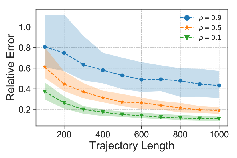
In the first experiment, we set , and we vary so that and for . Theorem 4.3 predicts that as increases towards one, the number of samples required for -relative error increases as well. Figure 2 corroborates this finding.
For our second experiment, we set so that the closed-loop response is simply . We generate random instances of as follows. For each , we generated instances by setting for all diagonal entries and independently for all upper triangular entries. We order the instances by , where and take the median. This results in , , and for , respectively. We then run LSTD on the three median instances, reporting the results in Figure 2. Once again, as increases, the required trajectory length increases, as suggested by Theorem 4.3. We note, however, that Theorem 4.3 appears to be conservative in predicting the actual scaling behavior with .
/* Estimate Q-function for K. */
/* Policy improvement step. */
5.2 Least-Squares Policy Iteration
We now describe our comparison of the Least-Squares Policy Iteration (LSPI) algorithm from Lagoudakis and Parr [24] to the model-based approaches of Dean et al. [11]. It is interesting to empirically compare the end-to-end sample complexity of model-free versus model-based methods for LQR in order to reach a specified controller cost, since our theoretical results in Section 4.2 suggest that LSPI can require more samples than the model-based approaches. We look at the same LQR instance from Dean et al., which is described by
| (5.1) |
We will consider both the discounted LQR problem with and the average cost LQR problem, given by
The choice of ensures that the closed-loop system with the optimal discounted controller is stable. Our metric of interest will be the relative error , where is the optimal infinite-horizon cost on either the discounted or average cost objective, and is the infinite-horizon cost of using the controller in feedback with the true system (5.1).
We run our experiments as follows. We collect independent trajectories of the system (5.1) excited by independent Gaussian noise of length . This produces a collection of tuples . We repeat this whole process times. In our experiments, we will refer to the value as the number of timesteps, and each set of tuples collected will be referred to as a trial. As in the previous experiment, we use the prefix of the data to report different values for the number of timesteps used. We now describe in more detail the different algorithms we evaluate.
LSPI.
For completeness, LSPI is described in Algorithm 1. LSPI relies on a variant of LSTD for -functions instead of value functions, which is described in Algorithm 2. To run LSPI, we need a starting controller . The trivial controller is insufficient, since the matrix is not stable, and hence does not induce a finite -function. This is a drawback of LSPI; a reasonable initialization must be chosen for the algorithm to work. For the purposes of comparison, we set such that the closed loop matrix and is hence a valid starting point for LSPI. Furthermore, the relative error for the discounted case and for the average cost case. When running LSPI for discounted cost (resp. average cost), if at any point we estimate a policy such that (resp. ) is not stable, we consider the algorithm as having failed and assign it a score of .
Nominal controller.
The nominal controller works by first estimating the state-transition matrices from the given trajectories via ordinary least-squares. With the estimates , we directly solve via algebraic Ricatti equations for the optimal discounted/average cost controllers under the assumption that the dynamics are exactly . We then check to see if the resulting costs with the nominal controller in feedback with the true system are finite, and assign a score of otherwise.
Common Lyapunov controller.
The common Lyapunov synthesis procedure is developed in Dean et al. as a semidefinite relaxation to the non-convex robust controller synthesis problem with static state-feedback. The advantage of the common Lyapunov controller over the nominal is that, if the program succeeds, it provides a certificate that the actual closed-loop system is stable (this is not guaranteed by the nominal controller, nor LSPI). The disadvatage is that this robustness guarantee typically trades off with performance. Since the formulation in Dean et al. is for the average cost setting, we only run the procedure in this setting. Because the procedure is a robust synthesis algorithm, it takes as input an upper bound on the estimation errors and . We use both the true errors and the true errors as the input bounds. The former showcases the best possible performance, and the latter simulates the non-parametric bootstrap method used in Dean et al. to compute these confidence bounds; their results suggest that the bootstrap over-estimates the true errors by roughly a factor of two. We solve the resulting semidefinite programs using cvxpy [12] with MOSEK [37] as the backend solver.
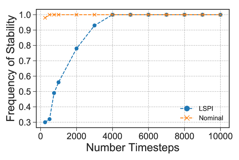

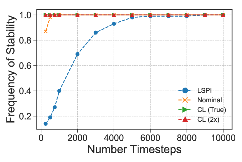
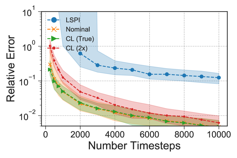
The results for the discounted LQR problem are shown in Figure 4 and Figure 4, and the results for the average cost LQR problem are shown in Figure 6 and Figure 6. We observe on the discounted problem that LSPI less robust and more sample inefficient than the nominal controller. In Figure 4, we observe that even with timesteps the frequency of stability for LSPI is worse than that of the nominal controller at timesteps. Similarly, in Figure 4, we see that the relative error achieved by LSPI at timesteps is comparable to that achieved by the nominal controller at timesteps. The qualitative differences between LSPI and the nominal controller remain the same when we move to the average cost controller. In Figure 6, we see that the nominal controller and the common Lyapunov controller given the actual error bounds perform the best, the common Lyapunov controller given the actual error bound performs slightly worse, and the performance of LSPI is substantially behind the rest, taking for instance over more samples compared to the nominal controller to achieve a relative error of .
6 Conclusion
We studied the number of samples needed for the LSTD estimator to return a -accurate solution in relative error for the value function associated to a fixed policy for LQR. In the process of deriving our result, we provided a concentration result for the minimum eigenvalue of a sample covariance matrix formed along the trajectory of a -mixing stochastic process. Empirically, we demonstrated that model-free policy iteration (LSPI) requires substantially more samples on certain LQR instances than the model-based methods from Dean et al. We hope our results encourage further investigation into the foundations of RL for continuous control problems. We now highlight some possible extensions of our work.
End-to-end guarantees.
Theorem 4.3 provides an upper bound on the estimation error of the value function for a fixed policy. While extending our analysis to estimating a fixed -function is straightforward, it is not as clear how to iterate this process. In particular, how many samples are needed until policy-iteration reaches a policy which receives an expected reward that is within additive or relative error to the optimal value? Our experiments in Section 5.2 suggest that the answer may be more than model-free methods, but it is not clear if this phenomenon is general or if there are instances where LSPI outperforms model-based methods. Can we establish conditions under which model-based methods will always outperform model-free methods?
Lower bounds.
Another interesting question is how sharp the bound in Theorem 4.3 is, especially in terms of its dependence on the spectral properties of . While our numerical experiments in Section 5.1 suggest that the qualitative behavior is correct, we do not have any algorithmic lower bounds for LSTD which confirm this rigorously. Furthermore, what are the information-theoretic lower bounds incurred by any RL algorithm for the LQR problem in terms of number of samples?
Other model-free RL estimators.
Policy gradient algorithms such as Trust Region Policy Optimization [42] have become increasingly popular for solving MDPs in robotics. How does the sample complexity of policy gradient or TRPO compare to LSPI and the model-based methods of Dean et al.?
Acknowledgements
We thank Orianna DeMasi, Vitaly Kuznetsov, Horia Mania, Max Simchowitz, Vikas Sindhwani, and Xinyan Yan for many helpful comments and suggestions. Part of this work was completed when ST was interning at Google Brain, New York, NY. BR is generously supported by NSF award CCF-1359814, ONR awards N00014-14-1-0024 and N00014-17-1-2191, the DARPA Fundamental Limits of Learning (Fun LoL) Program, a Sloan Research Fellowship, and a Google Faculty Award.
References
- [1] R. Adamczak, A. E. Litvak, A. Pajor, and N. Tomczak-Jaegermann. Sharp bounds on the rate of convergence of empirical covariance matrix. C. R., Math., Acad. Sci. Paris, 349, 2011.
- [2] A. Agarwal and J. C. Duchi. The Generalization Ability of Online Algorithms for Dependent Data. IEEE Transactions on Information Theory, 59(1), 2013.
- [3] A. Antos, C. Szepesvári, and R. Munos. Learning near-optimal policies with Bellman-residual minimization based fitted policy iteration and a single sample path. Machine Learning, 71(1), 2008.
- [4] D. P. Bertsekas. Dynamic Programming and Optimal Control, Vol. II. 2007.
- [5] V. I. Bogachev. Gaussian Measures. 2015.
- [6] J. Boyan. Least-Squares Temporal Difference Learning. In International Conference on Machine Learning, 1999.
- [7] S. J. Bradtke. Reinforcement Learning Applied to Linear Quadratic Regulation. In Neural Information Processing Systems, 1993.
- [8] S. J. Bradtke. Incremental Dynamic Programming for On-Line Adaptive Optimal Control. PhD thesis, University of Massachusetts Amherst, 1994.
- [9] S. J. Bradtke and A. G. Barto. Linear Least-Squares Algorithms for Temporal Difference Learning. Machine Learning, 22, 1996.
- [10] S. Bubeck, N. Cesa-Bianchi, and G. Lugosi. Bandits With Heavy Tail. IEEE Transactions on Information Theory, 59(11), 2013.
- [11] S. Dean, H. Mania, N. Matni, B. Recht, and S. Tu. On the Sample Complexity of the Linear Quadratic Regulator. arXiv:1710.01688, 2017.
- [12] S. Diamond and S. Boyd. CVXPY: A Python-embedded modeling language for convex optimization. Journal of Machine Learning Research, 17(83), 2016.
- [13] A. Farahmand, M. Ghavamzadeh, C. Szepesvári, and S. Mannor. Regularized Policy Iteration with Nonparametric Function Spaces. Journal of Machine Learning Research, 17(139), 2016.
- [14] A. Goldenshluger and A. Zeevi. Nonasymptotic bounds for autoregressive time series modeling. The Annals of Statistics, 29(2), 2001.
- [15] S. Gu, T. Lillicrap, Z. Ghahramani, R. E. Turner, and S. Levine. Q-Prop: Sample-Efficient Policy Gradient with An Off-Policy Critic. In International Conference on Learning Representations, 2017.
- [16] S. Gu, T. Lillicrap, I. Sutskever, and S. Levine. Continuous Deep Q-Learning with Model-based Acceleration. In International Conference on Machine Learning, 2016.
- [17] E. Jonas, Q. Pu, S. Venkataraman, I. Stoica, and B. Recht. Occupy the Cloud: Distributed Computing for the 99%. In ACM Symposium on Cloud Computing, 2017.
- [18] J. Kober, J. A. Bagnell, and J. Peters. Reinforcement Learning in Robotics: A Survey. The International Journal of Robotics Research, 32(11), 2013.
- [19] V. Koltchinskii and S. Mendelson. Bounding the smallest singular value of a random matrix without concentration. arXiv:1312.3580, 2013.
- [20] S. Krishnan, R. Fox, I. Stoica, and K. Goldberg. DDCO: Discovery of Deep Continuous Options for Robot Learning from Demonstrations. In Conference on Robot Learning, 2017.
- [21] V. Kuznetsov and M. Mohri. Learning Theory and Algorithms for Forecasting Non-Stationary Time Series. In Neural Information Processing Systems, 2015.
- [22] V. Kuznetsov and M. Mohri. Time Series Prediction and Online Learning. In Conference on Learning Theory, 2016.
- [23] V. Kuznetsov and M. Mohri. Generalization bounds for non-stationary mixing processes. Machine Learning, 106(1), 2017.
- [24] M. G. Lagoudakis and R. Parr. Least-Squares Policy Iteration. Journal of Machine Learning Research, 4, 2003.
- [25] A. Lazaric, M. Ghavamzadeh, and R. Munos. Finite-Sample Analysis of Least-Squares Policy Iteration. Journal of Machine Learning Research, 13, 2012.
- [26] S. Levine, C. Finn, T. Darrell, and P. Abbeel. End-to-End Training of Deep Visuomotor Policies. Journal of Machine Learning Research, 17(39), 2016.
- [27] S. Levine and V. Koltun. Learning Complex Neural Network Policies with Trajectory Optimization. In International Conference on Machine Learning, 2014.
- [28] S. Levine, P. Pastor, A. Krizhevsky, and D. Quillen. Learning Hand-Eye Coordination for Robotic Grasping with Deep Learning and Large-Scale Data Collection. arXiv:1603.02199, 2016.
- [29] S. Levine, N. Wagener, and P. Abbeel. Learning Contact-Rich Manipulation Skills with Guided Policy Search. In International Conference on Robotics and Automation, 2015.
- [30] T. P. Lillicrap, J. J. Hunt, A. Pritzel, N. Heess, T. Erez, Y. Tassa, D. Silver, and D. Wierstra. Continuous control with deep reinforcement learning. In International Conference on Learning Representations, 2016.
- [31] B. Liu, J. Liu, M. Ghavamzadeh, S. Mahadevan, and M. Petrik. Finite-Sample Analysis of Proximal Gradient TD Algorithms. In Uncertainty in Artificial Intelligence, 2015.
- [32] B. Liu, S. Mahadevan, and J. Liu. Regularized Off-Policy TD-Learning. In Neural Information Processing Systems, 2012.
- [33] D. J. McDonald, C. R. Shalizi, and M. Schervish. Nonparametric Risk Bounds for Time-Series Forecasting. Journal of Machine Learning Research, 18(32), 2017.
- [34] S. Mendelson and G. Paouris. On the singular values of random matrices. Journal of the European Mathematical Society, 16, 2014.
- [35] M. Mohri and A. Rostamizadeh. Rademacher Complexity Bounds for Non-I.I.D. Processes. In Neural Information Processing Systems, 2008.
- [36] M. Mohri and A. Rostamizadeh. Stability Bounds for Stationary -mixing and -mixing Processes. Journal of Machine Learning Research, 11, 2010.
- [37] MOSEK ApS. The MOSEK optimization toolbox for MATLAB manual. Version 7.1 (Revision 28)., 2015.
- [38] L. Prashanth, N. Korda, and R. Munos. Fast LSTD using stochastic approximation: Finite time analysis and application to traffic control. arXiv:1306.2557, 2014.
- [39] M. Rudelson and R. Vershynin. Smallest Singular Value of a Random Rectangular Matrix. Communications on Pure and Applied Mathematics, 62(12), 2009.
- [40] M. Rudelson and R. Vershynin. Hanson-Wright inequality and sub-gaussian concentration. Electronic Communications in Probability, 18(82), 2011.
- [41] T. Schaul, J. Quan, I. Antonoglou, and D. Silver. Prioritized Experience Replay. In International Conference on Learning Representations, 2016.
- [42] J. Schulman, S. Levine, P. Moritz, M. I. Jordan, and P. Abbeel. Trust Region Policy Optimization. In International Conference on Machine Learning, 2015.
- [43] J. Schulman, P. Moritz, S. Levine, M. Jordan, and P. Abbeel. High-Dimensional Continuous Control Using Generalized Advantage Estimation. In International Conference on Learning Representations, 2016.
- [44] N. Srivastava and R. Vershynin. Covariance estimation for distributions with moments. The Annals of Probability, 41(5), 2013.
- [45] R. S. Sutton and A. G. Barto. Reinforcement Learning. 1998.
- [46] R. Tedrake, T. W. Zhang, and H. S. Seung. Stochastic Policy Gradient Reinforcement Learning on a Simple 3D Biped. In International Conference on Intelligent Robots and Systems, 2004.
- [47] J. A. Tropp. Freedman’s inequality for matrix martingales. Electronic Communications in Probability, 16, 2011.
- [48] J. N. Tsitsiklis and B. V. Roy. An Analysis of Temporal-Difference Learning with Function Approximation. IEEE Transactions on Automatic Control, 42(5), 1997.
- [49] R. Vershynin. Introduction to the non-asymptotic analysis of random matrices. arXiv:1011.3027, 2011.
- [50] B. Yu. Rates of Convergence for Empirical Processes of Stationary Mixing Sequences. The Annals of Probability, 22(1), 1994.
- [51] H. Yu and D. P. Bertsekas. Convergence Results for Some Temporal Difference Methods Based on Least Squares. IEEE Transactions on Automatic Control, 54(7), 2009.
- [52] K. Zhou, J. C. Doyle, and K. Glover. Robust and Optimal Control. 1995.
Appendix A Gaussian Moment Lemmas
First, we present an elementary claim regarding the fourth moment of a non-isotropic multivariate Gaussian. For completeness, we provide a proof.
Proposition A.1.
Let , and two fixed symmetric matrices. We have that
Proof.
First, let be two fixed vectors. Let us compute
Fix an . We have that
On the other hand, for a fixed ,
Hence,
From this we conclude that
Now write the eigen-decompositions of and as and . We have that
Taking expectations,
∎
Next, we state a well-known result regarding Gaussian hypercontractivity.
Lemma A.2 (See e.g. Bogachev [5]).
Let be a degree polynomial and . For any , we have
Appendix B Proof of Lemma 4.4
This follows the development of Lazaric et al. [25]. From a given trajectory , let us define three matrices , , and as follows:
Above, , where is the transition dynamics of the MDP at state with action . The LSTD estimator is to find a such that
where is the vector of rewards received. Under the linear-architecture assumption, Bellman’s equation (4.1) implies that
| (B.1) |
Define the shift operator as
and define the empirical Bellman operator as
Let . We now see that the operator is contractive, where denotes the orthogonal projector onto the range of .
Proposition B.1.
For all , we have
Proof.
By definition, we have . By construction, we have that . The claim now follows since the projection operator is non-expansive in the -norm. ∎
Hence, by Banach’s fixed-point theorem, the operator has a unique fixed-point. It turns out the LSTD estimator is solving for this fixed point, as the following proposition demonstrates.
Proposition B.2 (Section 5.2, Lagoudakis and Parr [24]).
Suppose that has full column rank, and that satisfies
Then, we have that the fixed-point equation holds
Proof.
First, we observe the following equivalences
Next, it is easy to see that
Hence, the following relation holds
∎
Next is a structural result for the LSTD estimator.
Proposition B.3 (Theorem 1, Lazaric et al. [25]).
Let denote the LSTD estimator and suppose that has full column rank. We have that
Proof.
First, observe that
Above, (a) uses the fact that the LSTD estimator satisfies the fixed-point equation from Proposition B.2, and (b) uses the -contractive property of the operator from Proposition B.1. At this point, we have shown that
To finish the proof, we note that
where (a) comes from Bellman’s equation (B.1). The claim now follows. ∎