Dynamical bunching and density peaks in expanding Coulomb clouds

Abstract

Expansion dynamics of single-species, non-neutral clouds, such as electron bunches used in ultrafast electron microscopy, show novel behavior due to high acceleration of particles in the cloud interior. This often leads to electron bunching and dynamical formation of a density shock in the outer regions of the bunch. We develop analytic fluid models to capture these effects, and the analytic predictions are validated by PIC and N-particle simulations. In the space-charge dominated regime, two and three dimensional systems with Gaussian initial densities show bunching and a strong shock response, while one dimensional systems do not; moreover these effects can be tuned using the initial particle density profile and velocity chirp.

I Introduction

Non-neutral plasma systems arise in a variety of physical contexts ranging from astrophysicsArbañil et al. (2014); Maurya et al. (2015); Yousefi et al. (2014); accelerator technologies Bacci et al. (2014); Boine-Frankenheim et al. (2015); Whelan et al. (2016); Bernal et al. (2016); ion and neutron production Bulanov et al. (2002); Fukuda et al. (2009); Esirkepov et al. (2004); Kaplan (2015); Parks et al. (2001); Bychenkov et al. (2015); sources for electron and ion microscopyMurphy et al. (2014); Gahlmann et al. (2008); to high power vacuum electronicsBooske et al. (2011); Liu et al. (2015); Zhang and Lau (2016). Understanding of the dynamics of spreading of such systems is critical to the design of next generation technologies, and simple analytic models are particularly helpful for instrument design. As a result, substantial theoretical efforts have already been made in this veinJansen (1988); Reiser (1994); Batygin (2001); Bychenkov and Kovalev (2005); Grech et al. (2011); Kaplan et al. (2003); Kovalev and Bychenkov (2005); Last et al. (1997); Eloy et al. (2001); Krainov and Roshchupkin (2001); Morrison and Grant (2015); Boella et al. (2016). Specifically, free expansion of clouds of charged single-specie particles starting from rest have been well studied both analytically and computationallyLast et al. (1997); Eloy et al. (2001); Grech et al. (2011); Batygin (2001); Degtyareva et al. (1998); Siwick et al. (2002); Qian and Elsayed-Ali (2002); Reed (2006); Collin et al. (2005); Gahlmann et al. (2008); Tao et al. (2012); Portman et al. (2013, 2014); Michalik and Sipe (2006), and a number of studies have found evidence of the formation of a region of high-density, often termed a “shock”, on the periphery of the clouds under certain conditionsGrech et al. (2011); Kaplan et al. (2003); Kovalev and Bychenkov (2005); Last et al. (1997); Murphy et al. (2014); Reed (2006); Degtyareva et al. (1998).

One application of these theories that is of particular current interest is to high-density electron clouds used in next-generation ultrafast electron microscopy (UEM) developmentKing et al. (2005); Hall et al. (2014); Williams et al. (2017a). The researchers in the UEM and the ultrafast electron diffraction (UED) communities have conducted substantial theoretical treatment of initially extremely short bunches of thousands to ultimately hundreds of millions of electrons that operate in a regime dominated by a virtual cathode (VC) limitValfells et al. (2002); Luiten et al. (2004); King et al. (2005); Miller (2014); Tao et al. (2012) which is akin to the Child-Langmuir current limit for beams generated under the steady-state conditionsZhang and Lau (2016). These short bunches are often generated by photoemission, and such bunches inheret an initial profile similar to that of the driving laser pulse profile. Typically, the laser pulse has an in-plane, “transverse” extent that is of order one hundred microns and a duration on the order of fifty femtoseconds, and these parameters translate into an initial electron bunch with similar transverse extents and sub-micron widthsKing et al. (2005). After photoemission, the electrons are extracted longitudinally using either a DC or AC field typically in the 1-10 MV/mSrinivasan et al. (2003); Ruan et al. (2009); Van Oudheusden et al. (2010); Sciaini and Miller (2011) through tens of MV/mMusumeci et al. (2010); Weathersby et al. (2015); Murooka et al. (2011) ranges, respectively. However, the theoretical treatments of such “pancake-like” electron bunch evolution have largely focused on the longitudinal dimensionLuiten et al. (2004); Siwick et al. (2002); Qian and Elsayed-Ali (2002); Reed (2006); Collin et al. (2005), and the few studies looking at transverse dynamics have either assumed a uniform-transverse distributionCollin et al. (2005) or have looked at the effect of a smooth Gaussian-to-uniform evolution of the transverse profile on the evolution of the pulse in the longitudinal directionReed (2006); Portman et al. (2013). Of specific note, only one analytic study found any indication, a weak longitudinal signal, of a shockReed (2006).

(a) full z-x

(b) full x-y

(c) sliced z-x

(d) sliced x-y

(e) sliced radial evolution

Figure 1: (a-d.) Two dimensional projections of $1\times 10^{6}$ electron positions simulated with the N-particle code, COSY, for approximately 300 ps after injection with a Gaussian ($\sigma_{r}=100~{}\mu m$) transverse profile into a cavity with an electric field of 10 MV/m. Colors from white to red indicate electron density on a linear scale. (a.) and (b.) are projections of the full distribution to the x-z and x-y planes, respectively. (c.) and (d.) are x-z and x-y projections, respectively, of just the portion of the distribution within 20% of the standard deviation of the median value of y and z, respectively. Notice the ring-like substructure that is evident in the “slices”, (c.) and (d.) but absent from the full distribution projections, (a.) and (b.). (e.) N-particle radial-distributions obtained near the longitudinal median plane of the bunch at various times. Density is calculated by binning 1000 macroparticles and assigning the resulting density to the average radial position of those particles. The initial distribution is sampled from a Gaussian, and the square-like nature of the plot results from the discreteness of the bins. The sub-graph in the upper left corner shows the position of maximum density as a function of time, which is non-zero at initial time due to binning resulting in a non-zero minimum radial position. The sub-graph in the upper right shows the ratio of the maximum density to the density at the minimum $r$ value. Notice, the “phase transition” in the 45-80 ps range where the location of the non-zero, non-stochastic peak first appears well away from the origin.

On the other hand, an attractive theoretical observation is that an ellipsoidal cloud of cool, uniformly distributed charged particles has a linear electric field within the ellipsoid which results in maintenance of the uniform charge density as the cloud spreads Grech et al. (2011). In the accelerator community, such a uniform distribution is a prerequisite in employing techniques such as emittance compensationRosenzweig et al. (2006) as well as forming the basis of other theoretical analyses. It has long been proposed that such a uniform ellipsoid may be generated through proper control of the transverse profile of a short charged-particle bunch emitted from a source into vacuumLuiten et al. (2004), and experimental results have shown that an electron cloud emitted from a photocathode and rapidly accelerated into the highly-relativistic regime can develop into a final ellipsoidal profile characteristic of a uniform charge distributionMusumeci et al. (2008). Contrary to expectations from the free expansion work but consistent with the longitudinal analyses, this shadow lacks any indication of a peripheral region of high-density shocks. However, recent work has indicated that a substantial high density region may indeed form in the transverse directionWilliams et al. (2017b), and N-particle simulation results, as demonstrated in Fig. (1), demonstrate a rapidly-developed substantial ring-like shock circumscribing the median of the bunch when the bunch starts from sufficient density. Moreover, this shock corresponds to a region of exceedingly low brightness, or conversely, high, local temperature, and that experiments show that removal of this region results in a dramatic increase in the bunch brightnessWilliams et al. (2017b), which we term “Coulomb cooling” as it is similar to evaporative cooling in the fact that the “hottest” charged particles are removed from the distribution’s edge thus leaving behind a higher-quality, cooler bunch.

To understand Coulomb cooling, we first investigate this transverse shock. Here we demonstrate the formation of a ring-like shock within N-particle simulations Berz et al. (1987); Zhang et al. (2015) of electron bunches with initial transverse Gaussian profile and offer an explanation of why this phenomena has not been noted previously within the UED literature. We then utilize a Poisson fluid approach to derive analytic predictions for the expansion dynamics in planar (1D), cylindrical, and spherical geometries, and we derive conditions for the emergence of density peaks distinct from any initial density maximum. We show that peak formation has a strong dependence on dimension, with one dimensional systems less likely to form shocks, while in cylindrical and spherical geometries bunching is more typical. Particle-in-cell (PIC) methods, utilizing WARPFriedman et al. (2014), and N-particle simulation are then used to validate the analytical predictions for peak emergence.

II Observation of Transverse Shock

One reason that a transverse shock has not been seen previously in N-particle simulations is apparent in Fig. (1). We consider pancake electron bunches typical of 100keV ultrafast electron microscopy, and we consider the thin direction of the bunch to be the z-axis. Previous studies of the expansion dynamics of these bunches, including our own work, have looked at the projection of the particle density distribution to the x-z planeLuiten et al. (2004); Musumeci et al. (2008); Portman et al. (2014); Morrison et al. (2013); Li and Lewellen (2008). Fig. (1) shows that by projecting the distribution in this manner, and with the ability to statistically discern density fluctuations at about the 10% level, results in what appears to be a uniform distribution; however, by restricting the projection to only electrons near the median of the bunch, a restriction that can only be done computationally presently, results in evidence of a transverse ring-like density substructure near the median longitudinal (z) position.

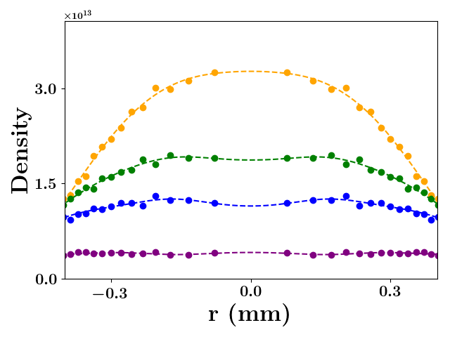
(a) $N=1,000$

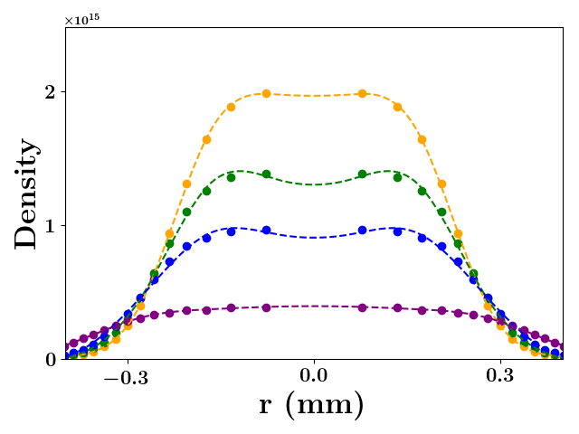
(b) $N=10,000$

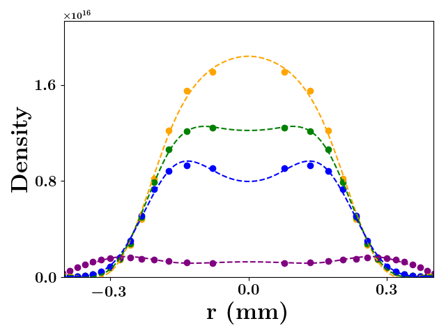
(c) $N=100,000$

Figure 2: Average density near the z-median of 30 simulations calculated from bunch profiles evaluated at different times: $5~{}\tau_{p}$ (yellow), $6~{}\tau_{p}$ (green), $7~{}\tau_{p}$ (blue), and $10~{}\tau_{p}$ (purple) where $\tau_{p}=2\pi\sqrt{\frac{m\epsilon_{0}}{ne^{2}}}$, $n=\frac{N}{\pi\sigma_{r}^{2}\sigma_{z}}$, and $\sigma_{z}\approx 0.4~{}\mu$m, for different values of the total number of electrons, $N$. Dotted lines represent spline fits of order 3 with 10 knots.

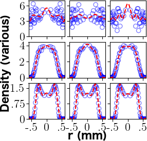
Figure 3: Density near the z-median of simulated pancake bunches with transverse Gaussian profiles ($\sigma_{r}=100~{}\mu$m) in an extraction field of 10 MV/m. Each figure is the transverse radial density of a section of width $\sigma_{z}\approx 0.4~{}\mu$m for different initial conditions and different numbers of electrons, at time $10~{}\tau_{p}$ where $\tau_{p}=2\pi\sqrt{\frac{m\epsilon_{0}}{ne^{2}}}$ is the plasma frequency; where $n=\frac{N}{\pi\sigma_{r}^{2}\sigma_{z}}$. The number of electrons in each horizontal panel is different and equal to $N=1,000$ (top), $N=10,000$ (middle), and $N=100,000$ (bottom). For the density at $10~{}\tau_{p}$, 30 cylindrical shells of equal volume and length $\sigma_{z}$ partitioned the distribution out to $0.6$ mm, and the numbers of electrons in each of these shells were used to calculate a density at the shell’s average radius. Due partially to the different numbers of electrons and partially due to the fact that the longer simulations, namely the simulation with $N=1000$, resulted in significantly more electrons migrating out of the analysis region as a result of the initial velocity spread , the density scales are different for the three rows in the figure: $\frac{1}{(0.1mm)^{3}}$ for the top row, $\frac{0.1}{(0.01mm)^{3}}$ for the middle row, and $\frac{1}{(0.01mm)^{3}}$ for the bottom row. Red dashed lines represent splines of order 3 with 10 knots. Notice the clear presence of a shock for the case $N=100,000$, an ambiguous shock at $N=10,000$, and essentially noise at $N=1,000$.

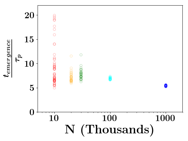
Figure 4: The emergence time divided by the plasma period as a function of the number of electrons in the initial Gaussian profile with $\sigma_{r}\approx 100~{}\mu$m and $\sigma_{z}\approx 0.4\mu$m. Emergence time was determined as the first time the density away from the inner-most-value exceeded the inner-most-value by 2%. Notice that the emergence time converges to about $5~{}\tau_{p}$ for high densities, but at low densities the emergence time has high variability with a median shifted to higher multiples of the plasma period.

To better understand when this shock emerges, simulations with the same distribution parameters ($\sigma_{r}\approx 100~{}\mu$m and $\Delta z\approx 0.4~{}\mu$m) but various numbers of electrons were run. The average radial density was calculated for 30 instances of bunches with 1 thousand, 10 thousand, and 100 thousand electrons. As can be seen in Fig. (2), the shock emergence is present for bunches with 100 thousand electrons but not for those with 1 thousand electrons. The case of bunches with 10 thousand electrons suggests the emergence of the shock, but the shock becomes less defined at later times. Fig (3) shows nine density profiles at time $10~{}\tau_{p}$, where $\tau_{p}$ represents the plasma period, with $\tau_{p}=2\pi\sqrt{\frac{m\epsilon_{0}}{ne^{2}}}$ and $n=\frac{N}{\pi\sigma_{r}^{2}\sigma_{z}}$. The dots in each figure indicate average densities in cylindrical rings, originating from three randomly chosen initial conditions (figures in each row) and for three values of the total number of electrons $N$: 1 thousand, 10 thousand, and 100 thousand electrons; for the top, middle, and bottom rows, respectively. These representative density plots support the conclusion that the shock is only present in the case of bunches with 100 thousand electrons; where the spline fit to the data indicates a significant peak removed from the center of the bunch in all instances examined. As expected, the density of bunches with one thousand electrons is noisy due to low statistics both from the small number of electrons in the simulation and the large proportion of electrons that spread beyond the analysis region due to the initial velocity spread; and the density profile of bunches with 10 thousand electron has a consistent general shape that fits well to the spline fit but lacks significant emergent peaks; which are the indicators of shock formation.

We define the emergence time as the time at which peaks indicative of a shock emerge in the dynamics of Coulomb clouds. Fig. (4) shows the dependence of the emergence time, and its variability, on the number of electrons in a bunch. It also shows very clearly that the emergence time is proportional to the plasma period, $\tau_{p}$. As can be seen in this figure, the spread in the emergence time is large for a bunch with 10 thousand electrons, but this spread decreases as the density of the bunch increases. For bunches with $N\geq 100,000$ the spread in the emergence time is small, moreover the emergence time appears to converge toward approximately $5~{}\tau_{p}$ at large $N$ (for Gaussian initial distributions). We note here that for Gaussian pulses with similar spatial and temporal extents, simulations at and above $10$ million electrons, a goal of the communityLessner et al. (2016), result in relativistic velocities as a result of the stronger space-charge effects. As the discussion here focuses on non-relativistic physics, we present data for up to 1 million electrons, where the velocity obtained from the self-field remains non-relativistic.

The results presented in Figs. 2-4 are a second reason that shock formation has not been seen previously in studies of electron bunches. Specifically, most work has been conducted using $\leq 10,000$ electrons with a transverse standard deviation of 100 $\mu$m, and in the regime where there is no consistent emergence of a shock. Moreover, the fact that the non-relativistic evolution of the bunch profile has a time scale proportional to the plasma period, a fact that we derive under special geometries later in this manuscript, means that higher density bunches result in faster, more consistent evolution of the transverse profile. In other words, the emergence time of a shock happens earlier as the density of the bunch is increased. Specifically, a transverse shock emerges at on the order of $50$ ps for an initially Gaussian profile ($\sigma_{r}=100~{}\mu$m with sub-micron length) with $10^{6}$ electrons, which is the number of electrons which is the current goal for the diffraction communityLessner et al. (2016). This implies that for modern bunches, this transverse shock is happening well within the photoemission gun before the onset of the relativistic regime. The goal of $10^{8}$ electrons for the imaging community needs to be further examined as the transverse velocity spread will be relativistic, but we expect to find this effect there as well, however we expect that it occurs at short times, of order a few picoseconds.

III 1D model

As noted in the introduction, formation of a shock in the longitudinal direction of an expanding pancake pulse has not been observed, and the analysis of Reed Reed (2006) demonstrates that this is true for cold initial conditions. Here we re-derive this result using an elementary method, which enables extension to include the possibility of an initial chirp; and we find chirp conditions at which shock formation in the longitudinal direction can occur.

Consider the non-relativistic spreading of an electron bunch in a one dimensional model, which is a good early time approximation to the longitudinal spreading of a pancake-shaped electron cloud generated at a photocathode. In one dimensional models, the density, $\rho$, only depends on one coordinate, which we take to be $z$. We also take $\rho$ to be normalized so that its integral is one. For the sake of readability, denote the position of a particle from the Lagrangian perspective to be $z=z(t)$ and $z_{0}=z(0)$. The acceleration of a Lagrangian particle is

$$a(z;t)=\frac{qQ_{\text{tot}}}{2m\epsilon_{0}}\delta\sigma$$ (1)

where $q$ is the charge of the particle (e.g. electron), $m$ is its mass, $Q_{\text{tot}}$ is the total charge in the bunch, and

$$\delta\sigma=\int_{-z}^{z}\rho(\tilde{z};t)d\tilde{z}$$ (2)

The key observation enabling analytic analysis is that if the flow of electrons is lamellar, so that there is no crossing of particle trajectories, then these integrals and the acceleration calculated from them are time independent and hence may be determined from the initial distribution. Therefore, we denote $a(z;t)=a_{0}$, $\rho_{0}=\rho(z;0)$, and $\delta\sigma=\int_{-z_{0}}^{z_{0}}\rho_{0}(\tilde{z})d\tilde{z}$. Moreover, due to the fact that for any particle trajectory, the acceleration is constant and given by $a_{0}$, the Lagrangian particle dynamics reduces to the elementary constant acceleration kinematic equation

$$z(t)=z_{0}+v_{0}t+{1\over 2}a_{0}t^{2}$$ (3)

where $v_{0}$ is the initial velocity of the charged particle that has initial position $z_{0}$. Notice that both $v_{0}$ and $a_{0}$ are functions of the initial position, $z_{0}$, and we shall see later that the derivatives of these parameters, $v^{\prime}=\frac{dv_{0}}{dz_{0}}$ and $a^{\prime}=\frac{da_{0}}{dz_{0}}$ are important in describing the relative dynamics of Langrangian particles starting at different initial positions. Moreover, the special case of $v_{0}=0$ everywhere, which we will call the cold-case, is commonly assumed in the literature, and we now examine this case in detail.

First we consider the speading charge distribution within the Eulerian perspective, where $z$ is an independent variable instead of it describing the trajectory of a particle. We denote the charge distribution at all times to be $Q_{\text{tot}}\rho(z;t)$ with $\rho(z;t)$ a unitless, probability-like density and $Q_{\text{tot}}$ the total charge per unit area in the bunch. Since particle number is conserved, we have

$$\rho(z;t)dz=\rho_{0}dz_{0}$$ (4)

so that in the non-relativistic case derived above

$$\rho(z,t) =\rho_{0}\left({dz\over dz_{0}}\right)^{-1}=\frac{\rho_{0}}{1+v_{0}^{\prime}t+\frac{1}{2}a_{0}^{\prime}t^{2}}$$ (5)

Notice that the derivative of the acceleration with respect to the initial position is directly proportional to the initial distribution, so that for initial distributions that are symmetric about the origin,

$$a_{0}^{\prime} =\frac{qQ_{\text{tot}}}{2m\epsilon_{0}}\frac{d{\delta\sigma}}{dz_{0}}$$

$$=\frac{qQ_{\text{tot}}}{m\epsilon_{0}}\rho_{0}$$ (6)

Plugging Eq. (III) into Eq. (5), we get

$$\rho(z,t) ={\rho_{0}\over 1+v_{0}^{\prime}t+\frac{qQ_{\text{tot}}}{2m\epsilon_{0}}\rho_{0}t^{2}}$$ (7)

$$\frac{d}{dz}\rho(z,t) =\frac{\rho_{0}^{\prime}\left(1+v_{0}^{\prime}t\right)-\rho_{0}v_{0}^{\prime\prime}t}{\left(1+v_{0}^{\prime}t+\frac{qQ_{\text{tot}}}{2m\epsilon_{0}}\rho_{0}t^{2}\right)^{3}}$$ (8)

where $\rho_{0}^{\prime}=\frac{d\rho_{0}}{dz_{0}}$ and $v_{0}^{\prime\prime}=\frac{d^{2}v_{0}}{dz_{0}^{2}}$. A detailed derivation of the second expression is in Appendix A.

For the cold-case, Eq. (7) reduces to the density evolution equation derived by ReedReed (2006) using different methods. Also, in the cold-case, Eq. (8) simplifies into a proportionality between the initial slope of the distribution and the slope of the distribution at any later time. Therefore, a charge distribution that is initially at rest and unimodal, i.e only a single initial location has non-zero density with $\rho_{0}^{\prime}=0$, never develops a dynamically generated second maximum. This explains why we should not expect to see an emergent shock in the longitudinal direction; provided the 1D model is applicable and cold initial conditions are valid.

However, if particles in the initial state have an initial velocity that depends on initial position, i.e. $v_{0}(z_{0})$, then density peaks will emerge at $z$ when $t=\frac{1}{v_{0}^{\prime\prime}\rho_{0}-v_{0}^{\prime}\rho_{0}^{\prime}}$. This occurs at positive time if $v_{0}^{\prime\prime}\rho_{0}>v_{0}^{\prime}\rho_{0}^{\prime}$. In the special case $v_{0}^{\prime\prime}\rho_{0}=v_{0}^{\prime}\rho_{0}^{\prime}$, the distribution may be reframed as a cold-case distribution starting from $t=-\frac{mc_{1}\epsilon_{0}}{qQ_{\text{tot}}}$ for some $z_{0}$-independent constant $c_{1}$ with velocity units when $\frac{mc_{1}^{2}\epsilon_{0}}{qQ_{\text{tot}}}<1$ or a distribution starting from a singularity with velocity distribution ${\tilde{v}}_{0}=c_{1}\left(\rho_{0}-\frac{1}{2}\delta\sigma\right)$. As noted earlier, the function $a_{0}(z_{0})$ is monotonically increasing as a function of distance from the center of the pulse, which means that electrons at the edges of the bunch always have larger accelerations away from the center of the pulse than electrons nearer the pulse center. Thus crossover, where an inner electron moves past an outer electron, cannot occur unless the initial velocities of inner electrons overcome this relative acceleration.

A practical case where crossover may be designed is where the initial distribution has an initial velocity chirp, i.e. $v_{0}=cz_{0}$ where $c$ has units of inverse time. Intuitively we can expect that the velocity chirp needs to be negative in order for crossover to occur. To find the crossover time, we consider the time at which two electrons that were initially apart, are at the same position at the same time. In this case it is straight forward to find the time at which crossover occurs by considering an electron at initial position $z_{0}$, and a second electron at position $z_{0}+\delta z_{0}$. Before either of these electrons experiences a crossover Eq. (3) is valid, and setting $z(z_{0},t_{x})=z(z_{0}+dz_{0},t_{x})$ reduces to,

$$At^{2}_{x}+Bt_{x}+1=0$$ (9)

where $A=\frac{q}{2m\epsilon_{0}}\rho_{0}(z_{0})$ and $B=\frac{dz}{dz_{0}}$. Solving the quadratic equation leads to the crossover time given by

$$t_{x} =\frac{-B\pm\sqrt{B^{2}-4A}}{2A}$$ (10)

Since $A$ is always positive, the square root is real only if $B^{2}$ is larger than $4A$. Moreover the time is only positive if $B$ is negative. Therefore crossover only occurs if the chirp has a negative slope, as expected on physical grounds. The conditions for tuning the chirp to produce crossover in 1D are then

$$\frac{dv_{0}}{dz_{0}} <0$$ (11)

$$\left|\frac{dv_{0}}{dz_{0}}\right| \geq\sqrt{\frac{2q}{m\epsilon_{0}}\rho_{0}(z_{0})})$$ (12)

The results above are applicable to the spreading in the longitudinal direction of non-relativistic pancake bunches, because the expression Eq. (3) is linear in acceleration. In that case, the position of a charged particle at any time can be calculated from a superposition of the contribution from the space-charge field and any external constant field such as a constant and uniform extraction field. In that case, the space charge field leads to spreading of the pulse, while the extraction field leads solely to an acceleration of the center of mass of the entire bunch. In that case the center of mass and spreading dynamics are independent and can be decoupled. The extension of the description above to asymmetric charge density functions is also straightforward, as is the inclusion of an image field at the photocathode. Moreover, inclusion of these effects does not change Eq. (7), Eq. (8), nor the conclusions we have drawn from them. These results apply generally to all times before the initial crossover event within the evolution of the bunch, and once crossover occurs, the distribution can be reset with a new Eq. (7) to follow further density evolution.

As we show in the next section the one-dimensional results do not apply, even qualitatively, to higher dimensions, as the constant acceleration situation is not valid and crossover can occur even with cold initial conditions, as demonstrated in the simulations presented in previous section. In the next section we present fluid models in higher dimensions where the origin of these new effects is evident.

IV Cylindrical and Spherical Models

The methodology for the cylindrical and spherical systems is similar so we develop the analysis concurrently.

Consider a non-relativistic evolving distribution $Q_{\text{tot}}\rho(r,t)$, where $\rho(r,t)$ is again taken to be the unitless particle distribution and $Q_{\text{tot}}$ is again the total charge in the bunch. In a system with cylindrical symmetry, the mean field equation of motion for a charge at $r\equiv r(t)$ is given by

$$\frac{d\vec{p}_{\text{r}}}{dt}={qQ_{\text{tot}}\lambda(r,t)\over 2\pi\epsilon_{0}r}\hat{r},$$ (13)

where $\vec{p}_{\text{r}}$ is the momentum of a Lagrangian particle, $\lambda(r,t)$ is the cummulative distribution function (cdf)

$$\lambda(r,t)=\int_{0}^{r}2\pi\tilde{r}\rho(\tilde{r},t)d\tilde{r}$$ (14)

and $Q_{\text{tot}}\lambda(r;t)$ is the charge inside radius $r$. Analogously in a system with spherical symmetry, the equation of motion for an electron at position $r$ is given by

$$\frac{d\vec{p}_{\text{r}}}{dt}={qQ_{\text{tot}}P(r,t)\over 4\pi\epsilon_{0}r^{2}}\hat{r},$$ (15)

where $P(r,t)=\int_{0}^{r}4\pi\tilde{r}^{2}\rho(\tilde{r},t)d\tilde{r}$ is the cdf and $Q_{\text{tot}}P(r;t)$ is the charge within the spherical shell of radius $r$. Notice, $r$ in Eq. (13) denotes the cylindrical radius while $r$ in Eq. (15) represents the spherical radius. In both cases, before any crossover occurs, the cdf of a Lagrangian particle is constant in time. For simplicity we write $\lambda(r,t)=\lambda(r_{0},0)\equiv\lambda_{0}$ and $P(r,t)=P(r_{0},0)\equiv P_{0}$ for a particle starting at $r_{0}\equiv r(0)$. In other words, since $Q_{\text{tot}}\lambda_{0}$ and $Q_{\text{tot}}P_{0}$ can be interpreted as the charge contained in the appropriate Gaussian surface, if we track the particle that starts at $r_{0}$, these contained charges should remain constant before crossover occurs. It is convenient to also define the average particle density to be $\bar{\rho}_{0}=\frac{\lambda_{0}}{\pi r_{0}^{2}}$ in the cylindrically symmetric case and $\bar{\rho}_{0}=\frac{3P_{0}}{4\pi r_{0}^{3}}$ in the spherically symmetric case. Notice that these average particle densities are a function solely of $r_{0}$, and we will use these parameters shortly. Eq. (13) and Eq. (15) may now be rewritten as, for the cylindrical and spherical cases respectively

$$\frac{dp_{r}}{dt} ={qQ_{\text{tot}}\lambda_{0}\over 2\pi\epsilon_{0}r},$$ (16)

$$\frac{dp_{r}}{dt} ={qQ_{\text{tot}}P_{0}\over 4\pi\epsilon_{0}r^{2}},$$ (17)

which apply for the period of time before particle crossover. Note that unlike the one dimensional case, in two and three dimensional systems the acceleration on a Lagrangian particle is not constant, and has a time dependence through the time dependent position $r=r(r_{0}:t)$ term in the denominator.

Since Eq. (16) and Eq. (17) represent the force on the particle in the cylindrical and spherical contexts, respectively, we can integrate over the particle’s trajectory to calculate the change in the particle’s energy. Integrating from $r_{0},0$ to $r,t$ gives for the cylindrical and spherical cases respectively

$$E(r,t)-E(r_{0},0) =\frac{qQ_{\text{tot}}\lambda_{0}}{2\pi\epsilon_{0}}ln\left(\frac{r}{r_{0}}\right)$$ (18)

$$E(r,t)-E(r_{0},0) =\frac{qQ_{\text{tot}}P_{0}}{4\pi\epsilon_{0}}\left(\frac{1}{r_{0}}-\frac{1}{r}\right)$$ (19)

where the term on the right side of the equality can be interpreted as the change in the potential energy within the self-field of the bunch.

These expressions are fully relativistic, and in the non-relativistic limit, we can derive implicit position-time relations for the particle by setting the energy difference equal to the non-relativisitic kinetic energy $mv^{2}/2$, and integrating. The details of this derivation have been placed in Appendix B, and the resulting expressions in the cold-case for the cylindrical and spherical systems are respectively

$$t =\frac{\bar{\tau}_{p,0}}{\pi}\frac{r}{r_{0}}F\left(\sqrt{ln\left(\frac{r}{r_{0}}\right)}\right)$$ (20)

$$t =\sqrt{\frac{3}{2}}\frac{\bar{\tau}_{p,0}}{2\pi}\left(\tanh^{-1}\left(\sqrt{1-\frac{r_{0}}{r}}\right)+\frac{r}{r_{0}}\sqrt{1-\frac{r_{0}}{r}}\right)$$ (21)

where $F(\cdot)$ represents the Dawson function and $\bar{\tau}_{p,0}$ represents the plasma period determined from the initial conditions: $\bar{\tau}_{p,0}=2\pi\sqrt{\frac{m\epsilon_{0}}{qQ_{\text{tot}}\bar{\rho}_{0}}}=\frac{2\pi}{{\bar{\omega}}_{0}}$, indicating that the appropriate time scale is the scaled plasma period as seen in Figs. (2) and (4) for the case of pancake bunches used in ultrafast electron diffraction systems. Eq. (21) and its derivation is equivalent to previous time-position relations reported in the literatureBoyer et al. (1989); Last et al. (1997) although the previous work did not identify the plasma period as the key time-scale of Coulomb spreading processes and cylindrical symmetry was not discussed (Eq. (20)).

The time-position relations detailed in the equations above depend solely on the amount of charge nearer to the origin than the point in question, i.e. $Q_{\text{tot}}\bar{\rho}_{0}$, and not on the details of the distribution. Notice however, that it is the difference between the time-position relationships of different locations where the details of the distribution become important and may cause neighboring particles to have interesting relative dynamics; leading to the possibility of shock formation in the density.

To translate the Lagrangian particle evolution equations above to an understanding of the dynamics of the charge density distribution, we generalize Eq. (5) to

$$\rho(r,t)=\rho_{0}\left(\left(\frac{r}{r_{0}}\right)^{d-1}{\frac{dr}{dr_{0}}}\right)^{-1}$$ (22)

where d is the dimensionality of the problem, i.e. 1 (planar symmetry), 2 (cylindrical symmetry), or 3 (spherical symmetry). The factor in the denominator, ${\frac{dr}{dr_{0}}}$, may be determined implicitly from the time-position relations above, and the details are presented in Appendix C. The resulting expressions for the density dynamics, in the cold case, for $d=2$ (cylindrical) and $d=3$ (spherical) cases are

$$\frac{dr}{dr_{0}} =\frac{r}{r_{0}}\left(1+D_{d}(r_{0})f_{\text{d}}\left(\frac{r}{r_{0}}\right)\right)$$ (23)

where

$$D_{d}=D_{d}(r_{0})=\frac{d}{2}\left(\frac{\rho_{0}}{\bar{\rho}_{0}}-1\right),$$ (24)

is a function only of the initial position. The functions $f_{d}$ for cylindrical systems is given by

$$f_{\text{2}}\left(\frac{r}{r_{0}}\right)=2\sqrt{\ln\left(\frac{r}{r_{0}}\right)}F\left(\sqrt{\ln\left(\frac{r}{r_{0}}\right)}\right),$$ (25)

while for systems with spherical symmetry we find

$$f_{\text{3}}\left(\frac{r}{r_{0}}\right)=\frac{r_{0}}{r}\sqrt{1-\frac{r_{0}}{r}}\tanh^{-1}(\sqrt{1-\frac{r_{0}}{r}})+1-\frac{r_{0}}{r}.$$ (26)

Note that these are functions of the ratio $r/r_{0}$. The functions $f_{d}$ can also be written as mixed functions of $r$ and $t$, specifically $f_{2}\left(\frac{r}{r_{0}}\right)=\frac{r_{0}}{r}\sqrt{\ln\left(\frac{r}{r_{0}}\right)}{\bar{\omega}}_{0}t$ and $f_{3}\left(\frac{r}{r_{0}}\right)=\frac{r_{0}}{r}\sqrt{1-\frac{r_{0}}{r}}{\bar{\omega}}_{0}t$. However, care must be used when using these mixed forms as $r$ is implicitly dependent on $t$. Here we work with these functions in terms of relative position, $\frac{r}{r_{0}}$. Substituting Eq. (23) into Eq. (22), we find that the density evolution in systems with cylindrical (d=2) and spherical symmetry(d=3) can be compactly written as

$$\rho(r;t) =\left(\frac{r_{0}}{r}\right)^{d}\frac{\rho_{0}}{1+D_{d}(r_{0})f_{\text{d}}\left(\frac{r}{r_{0}}\right)}$$ (27)

This expression is general and can be applied to arbitrary, spherically symmetric or cylindrically symmetric initial conditions.

Analogously to the 1D case the condition $\frac{dr}{dr_{0}}<0$ results in particle crossover. However, as detailed in Eq. (23), the sign of $\frac{dr}{dr_{0}}$ depends on the sign of $1+D_{d}(r_{0})f_{\text{d}}\left(\frac{r}{r_{0}}\right)$. It is very interesting to note that $D_{\text{d}}(r_{0})$ is the deviation from a uniform distribution function, so that the $D$ functions are solely functions of the initial conditions and are positive at locations where the local density is larger than the average density at $r_{0}$, and negative when the local density is smaller than the average density at $r_{0}$. On the other hand, the functions $f_{d}$ are functions of the evolution of the Langrangian particle. One immediate consequence of Eq.(27) is that for a uniform initial density distribution, for either cylindrical or spherical systems, the corresponding $D$ function is zero at every location where the original density is defined. Thus, the uniform density evolution in Eq. (22) reduces to the generally recognized expressions: $\rho(r,t)\pi r^{2}=\rho_{0}\pi r_{0}^{2}$ for the cylindrical case; and $\rho(r,t)\frac{4}{3}\pi r^{3}=\rho_{0}\frac{4}{3}\pi r_{0}^{3}$ in the spherical case. We provide additional details for the uniform distribution in the next section. However, Eq. (23) is general for any distribution before particle crossover, not just the uniform distribution.

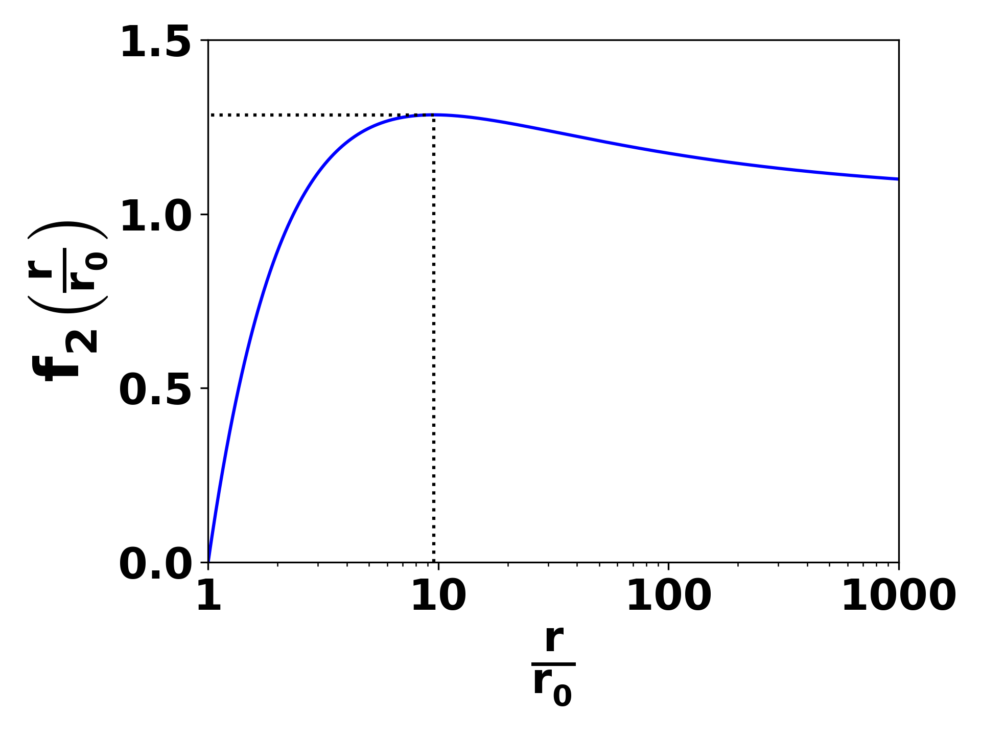
(a) $f_{\text{2}}\left(\frac{r(t)}{r(0)}\right)$

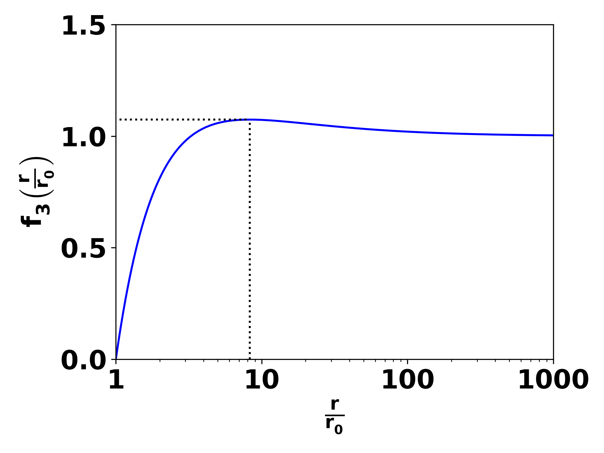
(b) $f_{\text{3}}\left(\frac{r(t)}{r(0)}\right)$

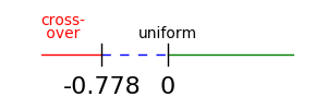
(c) $D_{\text{2}}(r(0))$ classification

(d) $D_{\text{3}}(r(0))$ classification

Figure 5: (a-b.) Plot of the functions $f_{\text{2}}$ and $f_{\text{3}}$ against $\frac{r}{r_{0}}$. Since particles are always moving away from the origin, $\frac{r}{r_{0}}>1$ for positive times and this ratio go to infinity for infinite time. Both functions have a similar character with a maximum in the $8-10~{}r_{0}$ range, and they both eventually approach one from above. Dashed lines in the plots indicate the location of the functions’ maxima. These functions allow us to analytically classify the distribution by the initial value of $D_{\text{d}}(r_{0})=\frac{d}{2}\left(\frac{\rho_{0}(r_{0})}{\bar{\rho}_{0}(r_{0})}-1\right)$ as is done in (c-d.). Specifically, crossover may occur at some time when $\frac{dr}{dr_{0}}<0$. For negative values of $D_{d}$ crossover first occurs at the maximum of $f_{d}$ and the value of $D_{d}$ at which that occurs is given in the schematics of (c,d). For values of $D_{d}$ that are more negative than this value, crossover will occurs at some time in some parts of the distrubiton. For the uniform distribution, $D(r_{0})=0$ for all points inside the distribution. The dashed blue line indicates expansion less quickly than the uniform distribution, while the green line indicates more rapid expansion than for the uniform distribution.

For a particle starting at position $r_{0}$ and having a deviation from uniform function $D_{\text{d}}(r_{0})$, crossover occurs when the particle is at a position, $r$, that satisfies $f_{\text{d}}\left(\frac{r}{r_{0}}\right)=-1/D_{d}(r_{0})$. Since every particle moves toward positive $r$, every particle will have a time for which it will assume every value of the function $f\left(\frac{r}{r_{0}}\right))$. The character of the two and three dimensional $f$’s are similar as can be seen in Fig (5) where the value of the function is plotted against $\frac{r}{r_{0}}$. Specifically, both functions increase to a maximum and then asymptote towards 1 from above. This means that all density positions eventually experience uniform-like scaling since $\lim_{r\to\infty}f_{d}(\frac{r}{r_{0}})=1$ results in Eq. (22) simplifying to $\rho\pi r^{2}=\rho_{0}\frac{\pi r_{0}^{2}}{1+D_{\text{d}}(r_{0})}$ and $\rho\frac{4}{3}\pi r^{3}=\rho_{0}\frac{\frac{4}{3}\pi r_{0}^{3}}{1+D_{\text{d}}(r_{0})}$ in the cylindrical and spherical cases, respectively, for large enough $r$. Notice, this uniform-like scaling does not mean that the distribution goes to the uniform distribution, which is what happens in 1D but need not happen under cylindrical and spherical geometries.

The main difference between the cylindrical and spherical symmetries are that the cylindrical function’s maximum is larger than the spherical function’s maximum; and we find $max(f_{\text{2}})\approx 1.28$ while $max(f_{\text{3}})\approx 1.07$. Moreover the maximum of the cylindrical function occurs at a larger value of $\frac{r_{0}}{r}$ than that of the spherical function; specifically $r\approx 9.54r_{0}$ instead of $r\approx 8.27r_{0}$, respectively. The first observation means cylindrical symmetry is more sensitive to the distribution than the spherical case, while the second observation indicates that if crossover is going to occur for a specific particle, it will occur before the $r$ value for which the corresponding $f$ function is maximum (i.e. $r\approx 9.54r_{0}$ or $r\approx 8.27r_{0}$), otherwise the particle will never experience crossover. From this reasoning, we obtain the earliest time for crossover by minimizing the time taken for a trajectory to reach the maximum of the function $f_{d}$, with the crossover constraint ${\frac{dr}{dr_{0}}}=0$. This may be achieved by using Lagrange multipliers or by running calculations for a series of values of $r/r_{0}$ to find the position at which crossover happens first. The mean field theory is valid before the minimum crossover time, and the results presented below are well below this time.

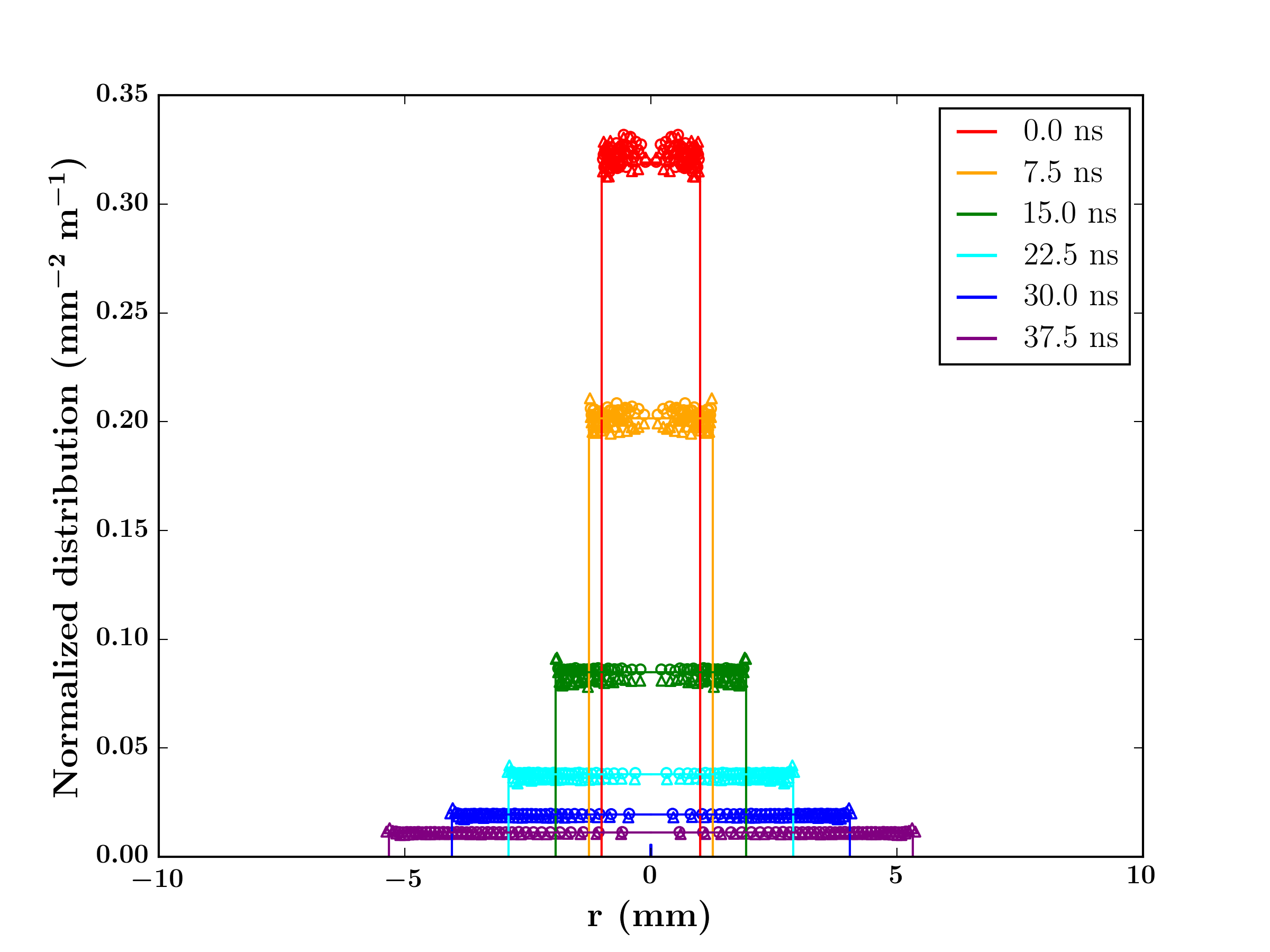
(a) cylindrical symmetry uniform

(b) spherical symmetry uniform

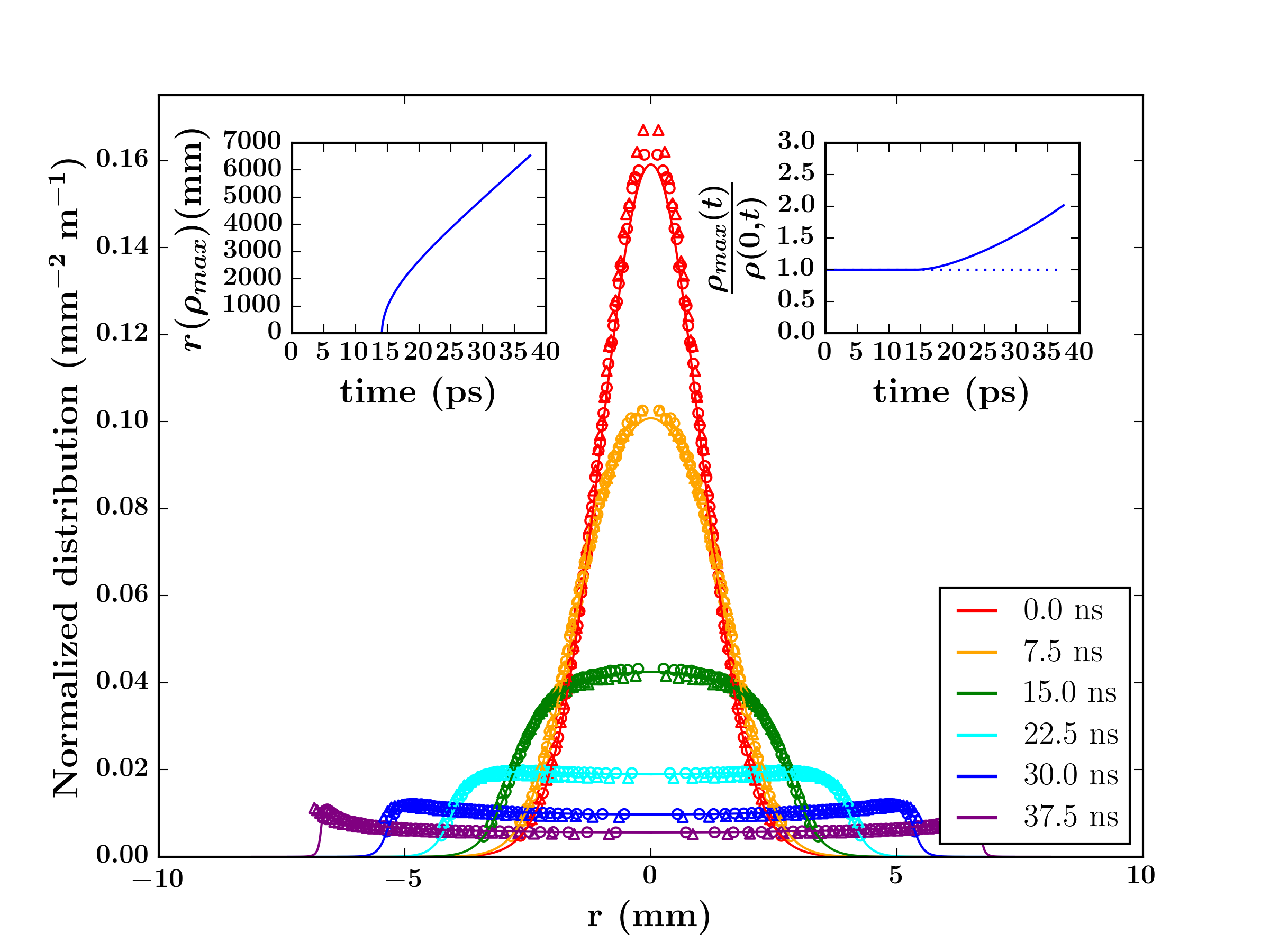
(c) cylindrical symmetry Gaussian

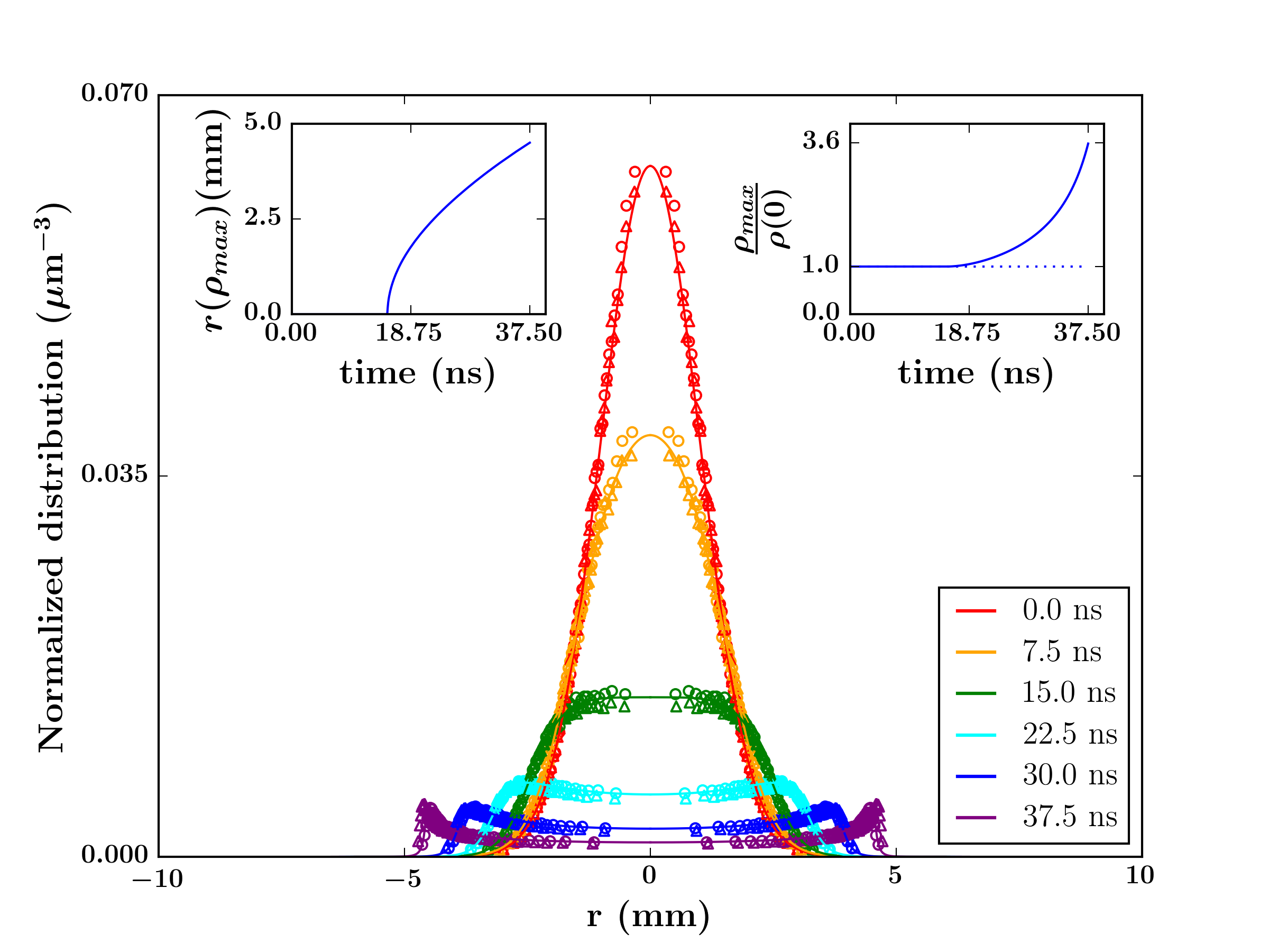
(d) spherical symmetry Gaussian

Figure 6: Analytical (solid line), PIC (circles), and N-particle (triangles) results of the normalized density evolution of (a.,c.) cylindrically and (b., d.) spherically symmetric (a., b.) uniform and (c.,d.) Gaussian distributions with $R=\sigma_{r}=1$ mm and $N$ of $1.875\times 10^{7}$, $2\times 10^{4}$, $3.75\times 10^{7}$, and $10^{5}$ electrons, respectively. The sub-graph in the upper left corner of (c.,d.) shows the analytic position of max density as a function of time, and the sub-graph in the upper right of (c.d.) shows the analytic ratio of the max density to the density at the minimum r value both. The corresponding analytic ratio for the uniform distribution is shown in this sub-graph as a dashed horizontal line at 1. Unsurprisingly, the PIC results and the analytical results, both mean-field models, are in almost perfect agreement, and the N-particle results are in surprisingly good agreement as well. Notice that the models predict peak formation on a time-scale dependent on the initial plasma frequency similar to the peak formation seen in the N-particle disc-like density evolution seen in Fig. (1(e)) and detailed in Fig. (4).

V Uniform and Gaussian Evolutions: Theory and Simulation

In this section, the mean field predictions are compared to the N-particle and PIC simulations. First we present the evolution of the initially-at-rest cylindrically- and spherically- symmetric uniform distribution of $1.875\times 10^{7}$ and $2\times 10^{4}$ electrons within radii’s of 1 mm (see Fig. (6(a,b)). Note, in this fairly trivial case, crossover should not occur and the analytic results should be valid mean-field-results for all time. Since $\rho_{0}={\bar{\rho}}_{0}$ in this case, $D_{d}(r_{0})=0$ and Eq. (27) reduces to

$$\rho(r;t)=\left(\frac{r_{0}}{r}\right)^{d}\rho_{0}(r_{0})$$ (28)

Notice that $r$ can be solved for a specific time using Eq. (20) or Eq. (21), depending on whether we are examining the cylindrically- or spherically- symmetric case, respectively, and due to ${\bar{\rho}}_{0}$’s independence from $r_{0}$, these equations need only be solved once for a give time to describe all $r$. Therefore, we may write $r=\alpha(t)r_{0}\equiv\alpha r_{0}$, where $\alpha$ is independent of $r_{0}$, and we immediately see that Eq. (28) can be written as $\rho(r;t)=\alpha^{d}\rho_{0}(r_{0})$ suggesting that the density simply scales with time as generally recognized by the community. We solve for $\alpha$ at 6 times, and present a comparison with both PIC and N-particle cylindrically- symmetric and spherically-symmetric simulations in Fig. (6(a,b)). As can be seen, despite the presence of initial density fluctuations arising from sampling, the simulated results follow the analytic results exceedingly well. Specifically, the distributions simply expand while remaining essentially uniform, and the analytic mean field formulation correctly calculates the rate of this expansion. While this comparison is arguably trivial, it is reassuring to see that our general equation reduces to a form that captures these dynamics.

Less trivial is the evolution of Gaussian distributions. We simulated $3.75\times 10^{7}$ and $10^{5}$ electrons for the cylindrical and spherical cases, respectively, using $\sigma_{r}=1~{}$ mm. Solving for the minimum crossover time, we get approximately 44 ns for each distribution. Therefore, we simulate for 37.5 ns, which is well before any crossover events.

For the Gaussian distributions we introduce the scaled radius variables $s=\frac{r}{\sqrt{2}\sigma_{r}}$ and $s_{0}=\frac{r_{0}}{\sqrt{2}\sigma_{r}}$, so that from Eq. (25) for the cylindrical and spherical cases we have,

$$D_{2}(s_{0}) =\frac{(1+s_{0}^{2})e^{-s_{0}^{2}}-1}{1-e^{-s_{0}^{2}}}$$ (29)

$$D_{3}(s_{0}) =\frac{(2s_{0}^{3}+3s_{0})e^{-s_{0}^{2}}-\frac{3\sqrt{\pi}}{2}\text{erf}(s_{0})}{\sqrt{\pi}\text{erf}(s_{0})-2s_{0}e^{-s_{0}^{2}}}$$ (30)

where erf is the well known error function. Putting these expressions into Eq. (27) we find for the cylindrical and spherical cases respectively

$$\rho(s;t) =\frac{\frac{s_{0}^{2}}{\pi s^{2}}e^{-s_{0}^{2}}}{1+2\frac{(1+s_{0}^{2})e^{-s_{0}^{2}}-1}{1-e^{-s_{0}^{2}}}\sqrt{\ln\left(\frac{s}{s_{0}}\right)}F\left(\sqrt{\ln\left(\frac{s}{s_{0}}\right)}\right)}$$ (31)

$$\rho(s;t) =\frac{\frac{s_{0}^{3}}{\pi^{\frac{3}{2}}s^{3}}e^{-s_{0}^{2}}}{1+\frac{(2s_{0}^{3}+3s_{0})e^{-s_{0}^{2}}-\frac{3\sqrt{\pi}}{2}\text{erf}(s_{0})}{\sqrt{\pi}\text{erf}(s_{0})-2s_{0}e^{-s_{0}^{2}}}\left(\frac{s_{0}}{s}\sqrt{1-\frac{s_{0}}{s}}\tanh^{-1}\left(\sqrt{1-\frac{s_{0}}{s}}\right)+1-\frac{s_{0}}{s}\right)}$$ (32)

To find $r(t)/r_{0}$ we solve Eq. (20) or Eq. (21), depending on whether we are examining the cylindrically- or spherically- symmetric cases, respectively; and for $\frac{r}{r_{0}}$, and for every time step, we calculate the predicted distribution at 5000 positions, $r$, corresponding to 5000 initial positions, $r_{0}$, evolved to time $t$. As can be seen in Fig. (6), both the cylindrically- and spherically- symmetric Gaussian distributions develop peaks similar to those seen in the simulations of expanding pancake bunches described in the first section of the paper. As can be seen in Fig. (6), both the PIC and the N-particle results match the analytical results very well. Notice, the primary differences between the cylindrically- and spherically- symmetric evolutions is in their rate of width expansion and the sharpness of the peak that forms, and both of these facets are captured by the analytic models.

VI Conclusions

In this work, we have shown that a shock occurs in the transverse, but not longitudinal, direction during expansion of pancake-like charged particle distributions typical of those use in ultrafast electron microscope (UEM) systems.

Fluid models for arbitrary initial distributions, Eq. (7), a generalization of a model already in the literature, showed that the formation of such a shock should not occur for any cold initial distribution in one dimension. This result is consistent with the finding that typically no shock is visible in the longitudinal direction dynamics of UEM bunches; however by tuning the initial velocity distribution it should be possible to generate a dynamic shock.

We generalized the fluid theory to cylindrical and spherical symmetries deriving implicit evolution equations for the charge density distributions Eq. (27). We analyzed these models for the advent of particle crossover, which occur for some distributions even when the initial distribution is cold due to the behavior of the Coulomb force in higher dimensions; and we found that the time scales associated with the space charge expansion are proportional to the plasma period. One interesting detailed observation is that in the case of cylindrical symmetry, the pre-factor of $\frac{\tau_{p}}{\pi}$ of Eq. (20) is roughly 0.3 while for the spherical symmetric case, corresponding prefactor in Eq. (21), $\sqrt{\frac{3}{2}}\frac{\tau_{p}}{2\pi}$, is roughly 0.2 plasma periods. Interestingly beam relaxation has been independently found to occur at roughly 0.25 the plasma periodWangler et al. (1985), which falls directly in the middle of our cylindrically and spherically symmetric models. The analytic theory predicts that emergence of a shock is distribution dependent, and as expected, a uniform initial distribution does not produce a shock. However we showed that electron bunches that are initially Gaussian distributed produce a shock well before the advent of particle crossover indicating that the emergence of a shock is well described by fluid models presented here. This is consistent with the observation of a shock in N-particle simulations of the transverse expansion of UEM pancake bunches (see Figs. 1-4).

To our knowledge, we have presented the first analytic derivation of the cold, single-species, non-neutral density evolution equations for cylindrical and spherical symmetries. These equations are general enough to handle any distribution under these symmetries, and can be used across specialties from accelerator technology, to electronics, to astrophysics. While simulation methods, like the N-particle and PIC codes used here are general tools, the insights provided by these simple analytical equations should provide fast and easy first-approximations for a number of calculations; while providing physical insights and parameter dependences that are more difficult to extract from purely computational studies.

The analysis presented here has been carried out for the non-relativistic regime; which is only valid for cases of sufficiently low density where the shock occurs prior to the electrons achieving relativistic velocities. For higher densities or other physical situations where the bunch becomes relativistic more quickly than the formation of this shock, a relativistic analysis is needed. On the other hand, for sufficiently high densities, i.e. approaching $10^{7}$ or more electrons in the pancake geometry used in this manuscript and typical in the UE field, relativistic effects in the transverse direction become important and need to be considered. The extension to fully relativistic cases will be addressed in future work.

We point out that Child-Langmuir current should not have these dynamic shocks except at the onset of the current before the steady-state condition sets in. Previous studies note the “hollowing” of a steady-state beam due to fringe field effectsLuginsland et al. (1996), but a steady state Child-Langmuir current is largely independent of emission parameters; so that this hollowing effect is not dynamical, but part of the continuous emission process itself, and is therefore a very different mechanism than the dynamic shocks we see here. It would be interesting to study the combined effects of steady state beam hollowing and dynamic shock formation in pancake bunches to determine if the combination of these processes provides new opportunities for optimization of beam properties.

The analytic models presented here treat free expansion whereas most applications have lattice elements to confine the bunches. Substantial work, in particular the particle-core model, has been very successful at predicting transverse particle halos of beamsGluckstern (1994); Wangler et al. (1998). This model assumes a uniform-in-space beam-core density called a Kapchinsky-Vladimirsky (KV) distribution due to its ease of theoretical treatment. Such an assumption is supported by the analysis presented here as we find that the distribution within the shock is nearly uniform. However, the particle-core models do not treat the initial distribution as having a large density on the periphery. It would be interesting to revisit such treatments with this new perspective although we would like to point out that the main effect the particle-core model attempts to capture, halos, occur even after aperturing the beamGluckstern (1994). Specifically, it should be possible to examine the effect of radial-focussing fields on the evolution of the three-dimensional distributions we have investigated here.

The experimental work that motivated this analysis, Williams et al. (2017b), not only predicted a shock but also a correlated decrease in brightness near the periphery. We emphasize that the mean-field equations used here explain the density shock only and do not provide a quantitative theory of the emittance and the Coulomb cooling achieved by removing the electrons in the shock. Specifically, the true emittance in the analytic models presented here remains zero for all time as all particles at a radius $r$ have velocity $\sqrt{\frac{2}{3}}\frac{r_{0}}{{\bar{\omega}}_{p,0}}\sqrt{1-\frac{r_{0}}{r}}$ resulting in zero local spread in velocity space. This perfect relationship between velocity and position means that the true emittance is zero even if the relation is non-linear; however, in such a non-linear chirp case, the rms emittance will not remain zero despite the true emittance being zero. Moreover, the analytic model does capture some of the rms emittance growth as a change in the distribution has a corresponding change on the variance measures used to determine the rms emittance. Specifically, a Gaussian distribution should have especially large emittance growth due to its evolution to a bimodal distribution, a distribution that is specifically problematic for variance measures. Such a large change in the emittance of the transverse Gaussian profile has been seen by LuitenLuiten et al. (2004) experimentally and us computationallyPortman et al. (2013, 2014). On the other hand, the perfectly uniform distribution does not change its distribution throughout its evolution and therefore should have zero rms emittance growth as the chirp exactly cancels out the expansion of the pulse at all times. Moreover, Luiten et al. found experimentally that the uniform distribution does have an increase in emittance although less than the Gaussian caselLuiten et al. (2004), an observation that is corroborated by our own work with PIC and N-particle calculationsPortman et al. (2013, 2014). The analytic formulation of mean-field theory presented here provides new avenues to treating emittance growth, by treating fluctuations to these equations in a systematic manner. This analysis will be presented elsewhere.

Acknowledgment This work was supported by NSF Grant 1625181, the College of Natural Science, the College of Communication Arts and Sciences, and the Provost’s office at Michigan State University. Computational resources were provided by the High Performance Computer Center at MSU. We thank Martin Berz and Kyoko Makino for their help with employing COSY as an N-particle code.

Appendix A 1D Density Derivative

In the main text, we argued

$$\rho(z)=\rho_{0}(z_{0})\left({dz\over dz_{0}}\right)^{-1}$$ (33)

To determine the slope of the density, we take the derivative with respect to the z coordinate

$$\frac{d}{dz}\rho(z) =\frac{d}{dz_{0}}\left(\rho_{0}(z_{0})\left(\frac{dz}{dz_{0}}\right)^{-1}\right)\left(\frac{dz}{dz_{0}}\right)^{-1}$$

$$=\frac{d}{dz_{0}}\left(\rho_{0}(z_{0})\right)\left(\frac{dz}{dz_{0}}\right)^{-2}-\rho_{0}(z_{0})\left(\frac{dz}{dz_{0}}\right)^{-3}\frac{d^{2}z}{dz_{0}^{2}}$$

$$=\frac{\frac{d}{dz_{0}}\left(\rho_{0}(z_{0})\right)\frac{dz}{dz_{0}}-\rho_{0}(z_{0})\frac{d^{2}z}{dz_{0}^{2}}}{\left(\frac{dz}{dz_{0}}\right)^{3}}$$ (34)

For the sake of conciseness, denote $\rho_{0}=\rho_{0}(z_{0})$, $\rho^{\prime}=\frac{d}{dz}\rho(z)$, $\rho_{0}^{\prime}=\frac{d}{dz_{0}}\rho_{0}$, $v_{0}^{\prime}=\frac{dv_{0}}{dz_{0}}$, and $v_{0}^{\prime\prime}=\frac{d^{2}v_{0}}{dz_{0}^{2}}$. From the main text, we have

$$\frac{dz}{dz_{0}} =1+v_{0}^{\prime}t+\frac{q}{2m\epsilon_{0}}\rho_{0}(z_{0})t^{2}$$ (35)

and from this it is straightforward to show

$$\frac{d^{2}z}{dz_{0}^{2}} =v_{0}^{\prime\prime}t+\frac{q}{2m\epsilon_{0}}\rho_{0}^{\prime}t^{2}$$ (36)

Subbing this back into Eq. (34), we get

$$\rho^{\prime} =\frac{\rho_{0}^{\prime}\left(1+v_{0}^{\prime}t+\frac{q}{2m\epsilon_{0}}\rho_{0}t^{2}\right)-\rho_{0}\left(v_{0}^{\prime\prime}t+\frac{q}{2m\epsilon_{0}}\rho_{0}^{\prime}t^{2}\right)}{\left(1+v_{0}^{\prime}t+\frac{q}{2m\epsilon_{0}}\rho_{0}t^{2}\right)^{3}}$$

$$=\frac{\rho_{0}^{\prime}\left(1+v_{0}^{\prime}t\right)-\rho_{0}v_{0}^{\prime\prime}t}{\left(1+v_{0}^{\prime}t+\frac{q}{2m\epsilon_{0}}\rho_{0}t^{2}\right)^{3}}$$ (37)

Appendix B Derivation of Time-location Relations

B.1 Integral form

Starting with the relativistic expression for change in particle energy derived in the main text

$$\text{cyl: }E(t)-E(0) =\frac{qQ_{tot}\lambda_{0}}{2\pi\epsilon_{0}}ln\left(\frac{r}{r_{0}}\right)$$ (38)

$$\text{sph: }E(t)-E(0) =\frac{qQ_{tot}P_{0}}{4\pi\epsilon_{0}}\left(\frac{1}{r_{0}}-\frac{1}{r}\right)$$ (39)

we approximate the energy change with a change in non-relativistic kinetic energy starting from rest

$$\text{cyl: }\frac{1}{2}mv^{2} =\frac{qQ_{tot}\lambda_{0}}{2\pi\epsilon_{0}}ln\left(\frac{r}{r_{0}}\right)$$ (40)

$$\text{sph: }\frac{1}{2}mv^{2} =\frac{qQ_{tot}P_{0}}{4\pi\epsilon_{0}}\left(\frac{1}{r_{0}}-\frac{1}{r}\right)$$ (41)

where $v=\frac{dr}{dt}$ are the velocity of the particle at time $t$ in the two or one of the three dimensional models, respectively, with the appropriate definition of $r$. Solving these equations for the velocity at time $t$, we get

$$\text{cyl: }\frac{dr}{dt} =\sqrt{\frac{qQ_{tot}\lambda_{0}}{\pi m\epsilon_{0}}ln\left(\frac{r}{r_{0}}\right)}$$ (42)

$$\text{sph: }\frac{dr}{dt} =\sqrt{\frac{qQ_{tot}P_{0}}{2\pi m\epsilon_{0}}\left(\frac{1}{r_{0}}-\frac{1}{r}\right)}$$ (43)

Separating the variables and integrating, we obtain

$$\text{cyl: }t =\int_{r_{0}}^{r}\frac{d\tilde{r}}{\sqrt{\frac{qQ_{tot}\lambda_{0}}{\pi m\epsilon_{0}}ln\left(\frac{\tilde{r}}{r_{0}}\right)}}$$ (44)

$$\text{sph: }t =\int_{r_{0}}^{r}\frac{d\tilde{r}}{\sqrt{\frac{qQ_{tot}P_{0}}{2\pi m\epsilon_{0}}\left(\frac{1}{r_{0}}-\frac{1}{\tilde{r}}\right)}}$$ (45)

Defining $a=\frac{qQ_{\text{tot}}}{\pi m\epsilon_{0}}$, we rewrite Eq. (44) and Eq. (45) as

$$\text{cyl: }t =\int_{r_{0}}^{r}\frac{d\tilde{r}}{\sqrt{a\lambda_{0}ln\left(\frac{\tilde{r}}{r_{0}}\right)}}$$ (46)

$$\text{sph: }t =\int_{r_{0}}^{r}\frac{d\tilde{r}}{\sqrt{\frac{aP_{0}}{2r_{0}}}\sqrt{1-\frac{r_{0}}{\tilde{r}}}}$$ (47)

B.2 Cylindrically-symmetric integral solution

We solve the sylindrically-symmetric integral first. Define $\tilde{u}=\sqrt{a\lambda_{0}ln\left(\frac{\tilde{r}}{r_{0}}\right)}$. Solving this equation for $\tilde{r}$ in terms of $\tilde{u}$, we see that $\tilde{r}=r_{0}e^{\frac{\tilde{u}^{2}}{a\lambda_{0}}}$. It is also straightforward to see that

$$d\tilde{u} =\frac{1}{2}\frac{1}{\sqrt{a\lambda_{0}ln\left(\frac{\tilde{r}}{r_{0}}\right)}}\frac{a\lambda_{0}}{\tilde{r}}d\tilde{r}$$

$$=\frac{1}{\sqrt{a\lambda_{0}ln\left(\frac{\tilde{r}}{r_{0}}\right)}}\frac{a\lambda_{0}}{2r_{0}}e^{\frac{-\tilde{u}^{2}}{a\lambda_{0}}}d\tilde{r}$$

Applying this change of coordinates to Eq. (46), we get

$$\text{cyl: }t =\int_{0}^{u}\frac{2r_{0}}{a\lambda_{0}}e^{\frac{\tilde{u}^{2}}{a\lambda_{0}}}d\tilde{u}$$

$$=\frac{2r_{0}}{a\lambda_{0}}e\int_{0}^{u}e^{\frac{\tilde{u}^{2}}{a\lambda_{0}}}d\tilde{u}$$

$$=\frac{2r_{0}}{\sqrt{a\lambda_{0}}}\int_{0}^{w}e^{\tilde{w}^{2}}d\tilde{w}$$ (48)

where $u=\sqrt{a\lambda_{0}ln\left(\frac{r}{r_{0}}\right)}$, $\tilde{w}=\frac{\tilde{u}}{\sqrt{a\lambda_{0}}}$, and $w=\sqrt{ln\left(\frac{r}{r_{0}}\right)}$. The remaining integral, $\int_{0}^{w}e^{\tilde{w}^{2}}d\tilde{w}$ can be written in terms of the well-studied Dawson function, $F(\cdot)$:

$$\int_{0}^{w}e^{\tilde{w}^{2}}d\tilde{w} =e^{w^{2}}F(w)$$

$$=\frac{r}{r_{0}}F\left(\sqrt{ln\left(\frac{r}{r_{0}}\right)}\right)$$ (49)

Subbing Eq. (49) back into Eq. (48) gives us our time-position relation

$$\text{cyl: }t =\frac{2r}{\sqrt{a\lambda_{0}}}F\left(\sqrt{ln\left(\frac{r}{r_{0}}\right)}\right)$$

$$=2\frac{r}{r_{0}}\sqrt{\frac{\pi r_{0}^{2}m\epsilon_{0}}{qQ_{\text{tot}}\lambda_{0}}}F\left(\sqrt{ln\left(\frac{r}{r_{0}}\right)}\right)$$

$$=2\frac{r}{r_{0}}\sqrt{\frac{m\epsilon_{0}}{qQ_{\text{tot}}\frac{\lambda_{0}}{\pi r_{0}^{2}}}}F\left(\sqrt{ln\left(\frac{r}{r_{0}}\right)}\right)$$

$$=2\frac{r}{r_{0}}\sqrt{\frac{m\epsilon_{0}}{qQ_{\text{tot}}{\bar{\rho}}_{0}}}F\left(\sqrt{ln\left(\frac{r}{r_{0}}\right)}\right)$$

$$=\frac{2}{{\bar{\omega}}_{p,0}}\frac{r}{r_{0}}F\left(\sqrt{ln\left(\frac{r}{r_{0}}\right)}\right)$$

$$=\frac{{\bar{\tau}}_{p,0}}{\pi}\frac{r}{r_{0}}F\left(\sqrt{ln\left(\frac{r}{r_{0}}\right)}\right)$$ (50)

where ${\bar{\rho}}_{0}=\frac{\lambda_{0}}{\pi r_{0}^{2}}$ and ${\bar{\omega}}_{p,0}=\sqrt{\frac{qQ_{\text{tot}}{\bar{\rho}}_{0}}{m\epsilon_{0}}}=\frac{2\pi}{{\bar{\tau}}_{p,0}}$.

B.3 Spherically-symmetric Integral Solution

We solve the spherically-symmetric integral with an analogous approach. Define $\tilde{u}=\sqrt{1-\frac{r_{0}}{\tilde{r}}}$ and solving for $\tilde{r}$ gives $\tilde{r}=\frac{r_{0}}{1-\tilde{u}^{2}}$. Thus

$$d\tilde{u} =\frac{1}{2}\frac{1}{\sqrt{1-\frac{r_{0}}{\tilde{r}}}}\frac{r_{0}}{\tilde{r}^{2}}d\tilde{r}$$

$$=\frac{1}{\sqrt{1-\frac{r_{0}}{\tilde{r}}}}\frac{(1-\tilde{u}^{2})^{2}}{2r_{0}}d\tilde{r}$$

Applying this change of coordinates to Eq. (47) with $u=\sqrt{1-\frac{r_{0}}{r}}$, we get

$$\text{sph: }t =\sqrt{\frac{2r_{0}}{aP_{0}}}\int_{0}^{u}\frac{2r_{0}}{(1-\tilde{u}^{2})^{2}}d\tilde{u}$$

$$=2\sqrt{\frac{2r_{0}^{3}}{aP_{0}}}\int_{0}^{u}\frac{1}{(1-\tilde{u}^{2})^{2}}d\tilde{u}$$

$$=2\sqrt{\frac{2r_{0}^{3}}{aP_{0}}}\left(\frac{1}{2}\tanh^{-1}\left(\tilde{u}\right)+\frac{1}{2}\frac{\tilde{u}}{1-\tilde{u}^{2}}\right)\bigg{\rvert}_{\tilde{u}=0}^{\tilde{u}=\sqrt{1-\frac{r_{0}}{r}}}$$

$$=\sqrt{\frac{2r_{0}^{3}}{aP_{0}}}\left(\tanh^{-1}\left(\sqrt{1-\frac{r_{0}}{r}}\right)+\frac{\sqrt{1-\frac{r_{0}}{r}}}{1-1+\frac{r_{0}}{r}}\right)$$

$$=\sqrt{\frac{2\pi r_{0}^{3}m\epsilon_{0}}{qQ_{\text{tot}}P_{0}}}\left(\tanh^{-1}\left(\sqrt{1-\frac{r_{0}}{r}}\right)+\frac{r}{r_{0}}\sqrt{1-\frac{r_{0}}{r}}\right)$$

$$=\sqrt{\frac{2}{3}}\sqrt{\frac{m\epsilon_{0}}{qQ_{\text{tot}}\frac{P_{0}}{\frac{4}{3}\pi r_{0}^{3}}}}\left(\tanh^{-1}\left(\sqrt{1-\frac{r_{0}}{r}}\right)\right.$$

$$\quad\quad\left.+\frac{r}{r_{0}}\sqrt{1-\frac{r_{0}}{r}}\right)$$

$$=\sqrt{\frac{2}{3}}\sqrt{\frac{m\epsilon_{0}}{qQ_{\text{tot}}{\bar{\rho}}_{0}}}\left(\tanh^{-1}\left(\sqrt{1-\frac{r_{0}}{r}}\right)\right.$$

$$\quad\quad\left.+\frac{r}{r_{0}}\sqrt{1-\frac{r_{0}}{r}}\right)$$

$$=\sqrt{\frac{2}{3}}\frac{1}{{\bar{\omega}}_{p,0}}\left(\tanh^{-1}\left(\sqrt{1-\frac{r_{0}}{r}}\right)+\frac{r}{r_{0}}\sqrt{1-\frac{r_{0}}{r}}\right)$$

$$=\sqrt{\frac{2}{3}}\frac{{\bar{\tau}}_{p,0}}{2\pi}\left(\tanh^{-1}\left(\sqrt{1-\frac{r_{0}}{r}}\right)+\frac{r}{r_{0}}\sqrt{1-\frac{r_{0}}{r}}\right)$$ (51)

where the solution to the integral was obtained with Mathematica’s online toolInc. and where ${\bar{\rho}}_{0}=\frac{P_{0}}{\frac{4}{3}\pi r_{0}^{3}}$ and ${\bar{\omega}}_{p,0}=\frac{qQ_{\text{tot}}{\bar{\rho}}_{0}}{m\epsilon_{0}}=\frac{2\pi}{{\bar{\tau}}_{p,0}}$.

Appendix C Derivation of Derivatives with Respect to Initial Position

As noted in the main text, much of the physics of distribution evolution in our models is captured in the term $\frac{dr}{dr_{0}}$. The procedure to derive the expressions for this derivative is to take the derivative of Eq. (B.2) and Eq. (51). We do this mathematics here.

C.1 The Cylindrically-symmetric Derivative

We begin by re-writing $t$ from Eq. (B.2) as

$$t =2r\sqrt{\frac{1}{a\lambda_{0}}}F\left(y\right)$$ (52)

where $y=\sqrt{ln\left(\frac{r}{r_{0}}\right)}=\sqrt{\ln\left(r\right)-\ln\left({r_{0}}\right)}$. So

$$\frac{dy}{dr_{0}} =\frac{1}{2y}\left(\frac{1}{r}\frac{dr}{dr_{0}}-\frac{1}{r_{0}}\right)$$ (53)

The Dawson function has the property $\frac{d}{dy}F(y)=1-2yF(y)=\left(\frac{1}{F(y)}-2y\right)F(y)$, and with the chain rule this becomes $\frac{d}{dr_{0}}F(y)=\left(\frac{1}{F(y)}-2y\right)\frac{dy}{dr_{0}}F(y)$. Using Eq. (53), this becomes

$$\frac{d}{dr_{0}}F\left(y\right) =\left(\frac{1}{F(y)}-2y\right)\frac{F(y)}{2y}\left(\frac{1}{r}\frac{dr}{dr_{0}}-\frac{1}{r_{0}}\right)$$

$$=F(y)\left(\frac{1}{2yF(y)}-1\right)\left(\frac{1}{r}\frac{dr}{dr_{0}}-\frac{1}{r_{0}}\right)$$ (54)

Also, note

$$\frac{d}{dr_{0}}\frac{1}{\sqrt{\lambda_{0}}} =-\frac{1}{2}\frac{1}{(\lambda_{0})^{3/2}}\frac{d\lambda_{0}}{dr_{0}}$$

$$=-\frac{1}{2\sqrt{\lambda_{0}}}\frac{d\ln(\lambda_{0})}{dr_{0}}$$ (55)

So

$$0 =\frac{dt}{dr_{0}}$$

$$=\frac{t}{r}\frac{dr}{dr_{0}}-\frac{1}{2}t\frac{d\ln(\lambda_{0})}{dr_{0}}+t\left(\frac{1}{2yF(y)}-1\right)\left(\frac{1}{r}\frac{dr}{dr_{0}}-\frac{1}{r_{0}}\right)$$

$$=\frac{t}{r}\frac{1}{2yF(y)}\frac{dr}{dr_{0}}-t\left(\frac{1}{2}\frac{d\ln(\lambda_{0})}{dr_{0}}+\left(\frac{1}{2yF(y)}-1\right)\frac{1}{r_{0}}\right)$$ (56)

which gives

$$\frac{dr}{dr_{0}} =2yF(y)r\left(\frac{1}{2}\frac{d\ln(\lambda_{0})}{dr_{0}}+\left(\frac{1}{2yF(y)}-1\right)\frac{1}{r_{0}}\right)$$

$$=\frac{r}{r_{0}}\left(1+\left(\frac{r_{0}}{2}\frac{d\ln(\lambda_{0})}{dr_{0}}-1\right)2yF(y)\right)$$

$$=\frac{r}{r_{0}}\left(1+\left(\frac{r_{0}}{2}\frac{2\pi r_{0}\rho_{0}}{\lambda_{0}}-1\right)2yF(y)\right)$$

$$=\frac{r}{r_{0}}\left(1+\left(\frac{\rho_{0}}{\frac{\lambda_{0}}{\pi r_{0}^{2}}}-1\right)2yF(y)\right)$$

$$=\frac{r}{r_{0}}\left(1+\left(\frac{\rho_{0}}{\bar{\rho}_{0}}-1\right)2\sqrt{\ln\left(\frac{r}{r_{0}}\right)}F\left(\sqrt{\ln\left(\frac{r}{r_{0}}\right)}\right)\right)$$ (57)

C.2 The Spherically-symmetric Derivatives

We begin by re-writing $t$ from Eq. (51) as

$$t =\sqrt{\frac{2r_{0}^{3}}{aP_{0}}}\left(\tanh^{-1}y+\frac{r}{r_{0}}y\right)$$ (58)

where $y=\sqrt{1-\frac{r_{0}}{r}}$. So

$$\frac{dy}{dr_{0}} =\frac{1}{2y}\left(\frac{r_{0}}{r^{2}}\frac{dr}{dr_{0}}-\frac{1}{r}\right)$$

$$=-\frac{1}{2yr}\left(1-\frac{r_{0}}{r}\frac{dr}{dr_{0}}\right)$$ (59)

Hence

$$\frac{d\tanh^{-1}y}{dr_{0}} =\frac{1}{1-y^{2}}\frac{dy}{dr_{0}}$$

$$=\frac{r}{r_{0}}\left(-\frac{1}{2yr}\left(1-\frac{r_{0}}{r}\frac{dr}{dr_{0}}\right)\right)$$

$$=-\frac{1}{2yr_{0}}\left(1-\frac{r_{0}}{r}\frac{dr}{dr_{0}}\right)$$ (60)

and

$$\frac{d\left(\frac{r}{r_{0}}y\right)}{dr_{0}} =\frac{y}{r_{0}}\frac{dr}{dr_{0}}-\frac{r}{r_{0}^{2}}y+\frac{r}{r_{0}}\frac{dy}{dr_{0}}$$

$$=\frac{1}{r_{0}}\left(\left(\frac{dr}{dr_{0}}-\frac{r}{r_{0}}\right)y-\frac{1}{2y}\left(1-\frac{r_{0}}{r}\frac{dr}{dr_{0}}\right)\right)$$

$$=\frac{1}{2yr_{0}}\left(2\left(\frac{dr}{dr_{0}}-\frac{r}{r_{0}}\right)\left(1-\frac{r_{0}}{r}\right)-1+\frac{r_{0}}{r}\frac{dr}{dr_{0}}\right)$$

Therefore

$$\frac{d\left(\tanh^{-1}y+\frac{r}{r_{0}}y\right)}{dr_{0}} =\frac{1}{yr_{0}}\left(\left(\frac{dr}{dr_{0}}-\frac{r}{r_{0}}\right)\left(1-\frac{r_{0}}{r}\right)\right.$$

$$\quad\quad\left.-1+\frac{r_{0}}{r}\frac{dr}{dr_{0}}\right)$$

$$=\frac{1}{yr_{0}}\left(\frac{dr}{dr_{0}}-\frac{r}{r_{0}}\right)$$

Also, similar to Eq. (55), $\frac{d}{dr_{0}}\frac{1}{\sqrt{P_{0}}}=-\frac{1}{2\sqrt{P_{0}}}\frac{d\ln(P_{0})}{dr_{0}}$. Putting this together we have

$$0 =\frac{dt}{dr_{0}}$$

$$=\frac{3}{2}\frac{t}{r_{0}}-\frac{t}{2}\frac{d\ln(P_{0})}{dr_{0}}+\sqrt{\frac{2r_{0}^{3}}{aP_{0}}}\frac{d\left(\tanh^{-1}y+\frac{r}{r_{0}}y\right)}{dr_{0}}$$

$$=\frac{3}{2}\frac{t}{r_{0}}-\frac{t}{2}\frac{d\ln(P_{0})}{dr_{0}}+\sqrt{\frac{2r_{0}^{3}}{aP_{0}}}\frac{1}{yr_{0}}\left(\frac{dr}{dr_{0}}-\frac{r}{r_{0}}\right)$$ (63)

Solving for $\frac{dr}{dr_{0}}$ we get

$$\frac{dr}{dr_{0}} =\frac{r}{r_{0}}-\frac{3y}{2}\left(\tanh^{-1}y+\frac{r}{r_{0}}y\right)$$

$$\quad\quad+\frac{yr_{0}}{2}\left(\tanh^{-1}y+\frac{r}{r_{0}}y\right)\frac{d\ln(P_{0})}{dr_{0}}$$

$$=\frac{r}{r_{0}}+\frac{3y}{2}\left(\frac{r_{0}}{3}\frac{d\ln(P_{0})}{dr_{0}}-1\right)\left(\tanh^{-1}y+\frac{r}{r_{0}}y\right)$$

$$=\frac{r}{r_{0}}\left(1+\frac{3}{2}\left(\frac{r_{0}}{3}\frac{4\pi r_{0}^{2}\rho_{0}}{P_{0}}-1\right)\left(\frac{r_{0}}{r}y\tanh^{-1}y+y^{2}\right)\right)$$

$$=\frac{r}{r_{0}}\left(1+\frac{3}{2}\left(\frac{\rho_{0}}{\frac{P_{0}}{\frac{4}{3}\pi r_{0}^{3}}}-1\right)\left(\frac{r_{0}}{r}\sqrt{1-\frac{r_{0}}{r}}\tanh^{-1}\left(\sqrt{1-\frac{r_{0}}{r}}\right)\right.\right.$$

$$\quad\quad\left.\left.+1-\frac{r_{0}}{r}\right)\right)$$

$$=\frac{r}{r_{0}}\left(1+\frac{3}{2}\left(\frac{\rho_{0}}{{\bar{\rho}}_{0}}-1\right)\left(\frac{r_{0}}{r}\sqrt{1-\frac{r_{0}}{r}}\tanh^{-1}\left(\sqrt{1-\frac{r_{0}}{r}}\right)\right.\right.$$

$$\quad\quad\left.\left.+1-\frac{r_{0}}{r}\right)\right)$$ (64)

References

- Arbañil et al. (2014) J. D. Arbañil, J. P. Lemos, and V. T. Zanchin, Physical Review D 89, 104054 (2014).
- Maurya et al. (2015) S. Maurya, Y. Gupta, S. Ray, and S. R. Chowdhury, The European Physical Journal C 75, 389 (2015).
- Yousefi et al. (2014) R. Yousefi, A. B. Davis, J. Carmona-Reyes, L. S. Matthews, and T. W. Hyde, Physical Review E 90, 033101 (2014).
- Bacci et al. (2014) A. Bacci, A. Rossi, et al., Nuclear Instruments and Methods in Physics Research Section A: Accelerators, Spectrometers, Detectors and Associated Equipment 740, 42 (2014).
- Boine-Frankenheim et al. (2015) O. Boine-Frankenheim, I. Hofmann, J. Struckmeier, and S. Appel, Nuclear Instruments and Methods in Physics Research Section A: Accelerators, Spectrometers, Detectors and Associated Equipment 770, 164 (2015).
- Whelan et al. (2016) B. Whelan, S. Gierman, L. Holloway, J. Schmerge, P. Keall, and R. Fahrig, Medical physics 43, 1285 (2016).
- Bernal et al. (2016) S. Bernal, B. Beaudoin, I. Haber, T. Koeth, Y. Mo, E. Montgomery, K. Rezaei, K. Ruisard, D. Sutter, H. Zhang, et al., in AIP Conference Proceedings, Vol. 1777 (AIP Publishing, 2016) p. 100003.
- Bulanov et al. (2002) S. Bulanov, T. Z. Esirkepov, F. Kamenets, Y. Kato, A. Kuznetsov, K. Nishihara, F. Pegoraro, T. Tajima, and V. Khoroshkov, Plasma Physics Reports 28, 975 (2002).
- Fukuda et al. (2009) Y. Fukuda, A. Y. Faenov, M. Tampo, T. Pikuz, T. Nakamura, M. Kando, Y. Hayashi, A. Yogo, H. Sakaki, T. Kameshima, et al., Physical review letters 103, 165002 (2009).
- Esirkepov et al. (2004) T. Esirkepov, M. Borghesi, S. Bulanov, G. Mourou, and T. Tajima, Physical review letters 92, 175003 (2004).
- Kaplan (2015) A. Kaplan, arXiv preprint arXiv:1503.06368 (2015).
- Parks et al. (2001) P. Parks, T. Cowan, R. Stephens, and E. Campbell, Physical Review A 63, 063203 (2001).
- Bychenkov et al. (2015) V. Y. Bychenkov, A. V. Brantov, E. A. Govras, and V. F. Kovalev, Physics-Uspekhi 58, 71 (2015).
- Murphy et al. (2014) D. Murphy, R. Speirs, D. Sheludko, C. Putkunz, A. McCulloch, B. Sparkes, and R. Scholten, Nature communications 5 (2014).
- Gahlmann et al. (2008) A. Gahlmann, S. T. Park, and A. H. Zewail, Physical Chemistry Chemical Physics 10, 2894 (2008).
- Booske et al. (2011) J. H. Booske, R. J. Dobbs, C. D. Joye, C. L. Kory, G. R. Neil, G.-S. Park, J. Park, and R. J. Temkin, IEEE Transactions on Terahertz Science and Technology 1, 54 (2011).
- Liu et al. (2015) Y. Liu, P. Zhang, S. Chen, and L. Ang, Physical Review Special Topics-Accelerators and Beams 18, 123402 (2015).
- Zhang and Lau (2016) P. Zhang and Y. Lau, Journal of Plasma Physics 82 (2016).
- Jansen (1988) G. H. Jansen, Coulomb interactions in particle beams [book] (Technische Universiteit Delft, Delft, 1988).
- Reiser (1994) M. Reiser, Theory and Design of Charged Particle Beams (John Wiley & Sons, New York, 1994).
- Batygin (2001) Y. K. Batygin, Physics of Plasmas 8, 3103 (2001).
- Bychenkov and Kovalev (2005) V. Y. Bychenkov and V. Kovalev, Plasma physics reports 31, 178 (2005).
- Grech et al. (2011) M. Grech, R. Nuter, A. Mikaberidze, P. Di Cintio, L. Gremillet, E. Lefebvre, U. Saalmann, J. M. Rost, and S. Skupin, Physical Review E 84, 056404 (2011).
- Kaplan et al. (2003) A. E. Kaplan, B. Y. Dubetsky, and P. Shkolnikov, Physical review letters 91, 143401 (2003).
- Kovalev and Bychenkov (2005) V. Kovalev and V. Y. Bychenkov, Journal of Experimental and Theoretical Physics 101, 212 (2005).
- Last et al. (1997) I. Last, I. Schek, and J. Jortner, The Journal of chemical physics 107, 6685 (1997).
- Eloy et al. (2001) M. Eloy, R. Azambuja, J. Mendonca, and R. Bingham, Physics of Plasmas 8, 1084 (2001).
- Krainov and Roshchupkin (2001) V. Krainov and A. Roshchupkin, Physical Review A 64, 063204 (2001).
- Morrison and Grant (2015) J. Morrison and E. Grant, Physical Review A 91, 023423 (2015).
- Boella et al. (2016) E. Boella, B. P. Paradisi, A. D’Angola, L. O. Silva, and G. Coppa, Journal of Plasma Physics 82, 905820110 (2016).
- Degtyareva et al. (1998) V. P. Degtyareva, M. A. Monastyrsky, M. Y. Schelev, and V. A. Tarasov, Optical Engineering 37, 2227 (1998).
- Siwick et al. (2002) B. J. Siwick, J. R. Dwyer, R. E. Jordan, and R. J. Dwayne Miller, Journal of Applied Physics 92, 1643 (2002).
- Qian and Elsayed-Ali (2002) B.-L. Qian and H. E. Elsayed-Ali, Journal of Applied Physics 91, 462 (2002).
- Reed (2006) B. W. Reed, Journal of Applied Physics 100, 034916 (2006).
- Collin et al. (2005) S. Collin, M. Merano, M. Gatri, S. Sonderegger, P. Renucci, J.-D. Ganiere, and B. Deveaud, Journal of applied physics 98, 094910 (2005).
- Tao et al. (2012) Z. Tao, H. Zhang, P. Duxbury, M. Berz, and C.-Y. Ruan, Journal of Applied Physics 111, 044316 (2012).
- Portman et al. (2013) J. Portman, H. Zhang, Z. Tao, K. Makino, M. Berz, P. Duxbury, and C.-Y. Ruan, Applied Physics Letters 103, 253115 (2013).
- Portman et al. (2014) J. Portman, H. Zhang, K. Makino, C. Ruan, M. Berz, and P. Duxbury, Journal of Applied Physics 116, 174302 (2014).
- Michalik and Sipe (2006) A. Michalik and J. Sipe, Journal of applied physics 99, 054908 (2006).
- King et al. (2005) W. E. King, G. H. Campbell, A. Frank, B. Reed, J. F. Schmerge, B. J. Siwick, B. C. Stuart, and P. M. Weber, Journal of Applied Physics 97, 111101 (2005).
- Hall et al. (2014) E. Hall, S. Stemmer, H. Zheng, Y. Zhu, and G. Maracas, Future of Electron Scattering and Diffraction, Tech. Rep. (US Department of Energy, Washington, DC (United States), 2014).
- Williams et al. (2017a) J. Williams, F. Zhou, T. Sun, K. Chang, K. Makino, M. Berz, P. Duxbury, and C.-Y. Ruan, Structural Dynamics 4 (2017a).
- Valfells et al. (2002) A. Valfells, D. Feldman, M. Virgo, P. O’shea, and Y. Lau, Physics of Plasmas (1994-present) 9, 2377 (2002).
- Luiten et al. (2004) O. J. Luiten, S. B. V. D. Geer, M. J. D. Loos, F. B. Kiewiet, and M. J. V. D. Wiel, Physical review letters 93, 094802 (2004).
- Miller (2014) R. D. Miller, Science 343, 1108 (2014).
- Srinivasan et al. (2003) R. Srinivasan, V. Lobastov, C.-Y. Ruan, and A. Zewail, Helvetica Chimica Acta 86, 1761 (2003).
- Ruan et al. (2009) C.-Y. Ruan, Y. Murooka, R. K. Raman, R. A. Murdick, R. J. Worhatch, and A. Pell, Microscopy and Microanalysis 15, 323 (2009).
- Van Oudheusden et al. (2010) T. Van Oudheusden, P. Pasmans, S. Van Der Geer, M. De Loos, M. Van Der Wiel, and O. Luiten, Physical review letters 105, 264801 (2010).
- Sciaini and Miller (2011) G. Sciaini and R. D. Miller, Reports on Progress in Physics 74, 096101 (2011).
- Musumeci et al. (2010) P. Musumeci, J. Moody, C. Scoby, M. Gutierrez, M. Westfall, and R. Li, Journal of Applied Physics 108, 114513 (2010).
- Weathersby et al. (2015) S. Weathersby, G. Brown, M. Centurion, T. Chase, R. Coffee, J. Corbett, J. Eichner, J. Frisch, A. Fry, M. Gühr, N. Hartmann, C. Hast, R. Hettel, R. K. Jobe, E. N. Jongewaard, J. R. Lewandowski, R. K. Li, A. M. Lindenberg, I. Makasyuk, J. E. May, D. McCormick, M. N. Nguyen, A. H. Reid, X. Shen, K. Sokolowski-Tinten, T. Vecchione, S. L. Vetter, J. Wu, J. Yang, D. H. A., and X. J. Wang, Review of Scientific Instruments 86, 073702 (2015).
- Murooka et al. (2011) Y. Murooka, N. Naruse, S. Sakakihara, M. Ishimaru, J. Yang, and K. Tanimura, Applied Physics Letters 98, 251903 (2011).
- Rosenzweig et al. (2006) J. Rosenzweig, A. Cook, R. England, M. Dunning, S. Anderson, and M. Ferrario, Nuclear Instruments and Methods in Physics Research Section A: Accelerators, Spectrometers, Detectors and Associated Equipment 557, 87 (2006).
- Musumeci et al. (2008) P. Musumeci, J. T. Moody, R. J. England, J. B. Rosenzweig, and T. Tran, Physical review letters 100, 244801 (2008).
- Williams et al. (2017b) J. Williams, F. Zhou, T. Sun, P. Duxbury, S. Lund, B. Zerbe, and C.-Y. Ruan, Bulletin of the American Physical Society 62 (2017b).
- Berz et al. (1987) M. Berz, H. Hoffmann, and H. Wollnik, Nuclear Instruments and Methods in Physics Research Section A: Accelerators, Spectrometers, Detectors and Associated Equipment 258, 402 (1987).
- Zhang et al. (2015) H. Zhang, J. Portman, Z. Tao, P. Duxbury, C.-Y. Ruan, K. Makino, and M. Berz, Microscopy and Microanalysis 21, 224 (2015).
- Friedman et al. (2014) A. Friedman, R. H. Cohen, D. P. Grote, S. M. Lund, W. M. Sharp, J.-L. Vay, I. Haber, and R. A. Kishek, IEEE Transactions on Plasma Science 42, 1321 (2014).
- Morrison et al. (2013) V. R. Morrison, R. P. Chatelain, C. Godbout, and B. J. Siwick, Optics express 21, 21 (2013).
- Li and Lewellen (2008) Y. Li and J. W. Lewellen, Physical review letters 100, 074801 (2008).
- Lessner et al. (2016) E. Lessner, X. Wang, and P. Musumeci, Report of the Basic Energy Sciences Workshop on the Future of Electron Sources, (SLAC National Accelerator Laboratory, 2016).
- Boyer et al. (1989) K. Boyer, T. Luk, J. Solem, and C. Rhodes, Physical Review A 39, 1186 (1989).
- Wangler et al. (1985) T. Wangler, K. Crandall, R. Mills, and M. Reiser, IEEE Transactions on Nuclear Science 32, 2196 (1985).
- Luginsland et al. (1996) J. Luginsland, Y. Lau, and R. Gilgenbach, Physical review letters 77, 4668 (1996).
- Gluckstern (1994) R. L. Gluckstern, Physical review letters 73, 1247 (1994).
- Wangler et al. (1998) T. Wangler, K. Crandall, R. Ryne, and T. Wang, Physical review special topics-accelerators and beams 1, 084201 (1998).
- (67) W. R. Inc., “Mathematica, Version 11.1,” Champaign, IL, 2017.