Generalized W-state of four qubits with exclusively threetangle

Abstract

We single out a class of states possessing only threetangle but distributed all over four qubits. This is a three-site analogue of states from the $W$-class, which only possess globally distributed pairwise entanglement as measured by the concurrence. We perform an analysis for four qubits, showing that such a state indeed exists. To this end we analyze specific states of four qubits that are not convexly balanced as for $SL$ invariant families of entanglement, but only affinely balanced. For these states all possible $SL$-invariants vanish, hence they are part of the $SL$ null-cone. Instead, they will possess at least a certain unitary invariant.

As an interesting byproduct it is demonstrated that the exact convex roof is reached in the rank-two case of a homogeneous polynomial $SL$-invariant measure of entanglement of degree $2m$, if there is a state which corresponds to a maximally $m$-fold degenerate solution in the zero-polytope that can be combined with the convexified minimal characteristic curve to give a decomposition of $\rho$. If more than one such state does exist in the zero polytope, a minimization must be performed. A better lower bound than the lowest convexified characteristic curve is obtained if no decomposition of $\rho$ is obtained in this way.

I Introduction

W-states are at the borderline between three distinct and important features of multipartite entanglement: pure W-states are satisfying the Coffman-Kundu-Wootters inequalityCoffman et al. (2000); Osborne and Verstraete (2006) as an equalityCoffman et al. (2000), they appear as representative of one of two classes of entanglementDür et al. (2000) for three qubits, and it is seen to be related to a ladder from $SL$ invariance to $U$ invarianceJohansson et al. (2014) for an arbitrary number of qubits. Indeed, three qubits have been shown to separate into the GHZ-class which is detected by the threetangleCoffman et al. (2000) and the remaining W-class sharing entanglement among two parties onlyCoffman et al. (2000). A further peculiarity of the $q$ qubit W-state is hence that it has no $SL$ invariant $n$-tangle with $n>2$ Osterloh and Siewert (2006, 2010).
It is therefor reasonable to ask the following question: do such states also exist for $q$ qubits and an arbitrary $n<q$; in other words: are there certain $q$ qubit states possessing only $n$-tangle? The corresponding states should in particular have no $SL$-invariant, we call it $q$-tangle, (with a $(2m,0)$ bidegree of unitary invariants) and thus be part of the $SL$ null-cone. The $SL$ null-cone, however, has a finer structure which is classified by further $SU$ invariants with a general bidegree $(2m-l,l)$ (see e.g. Luque et al. (2007)). $SU$-invariants of bidegree $(2m-l,l)$ are $(2m-l)$-linear in the wave-function $\psi$ and $l$-linear in its complex conjugate $\psi^{*}$ (or vice-versa). Every state which lies outside the null-cone must futhermore have a part which is balancedOsterloh and Siewert (2010) or equivalently termed c-balanced (c for convex) in Ref. Johansson et al. (2014). In contrast, there are those states which are a-balanced (a for affine) without being c-balanced. These states have been singled out having discrete topological phases under the cyclic local $SU$ group-operationJohansson et al. (2012) and emerge from the c-balanced states by means of partial spin flips Johansson et al. (2014). Simple examples are the states in the $SL$ W-class

$$|\psi_{\rm{W-class}}\rangle=a_{0}|000\rangle+a_{1}|100\rangle+a_{2}|010\rangle+a_{3}|001\rangle$$ (1)

for three qubits which do possess a $SU$ $(3,1)$-invariant. These states, by means of a partial spin flip, are connected to the $(4,0)$-invariant states which are in the $SL$-invariant $GHZ$-class

$$|\psi_{\rm{GHZ-class}}\rangle=a_{0}|111\rangle+a_{1}|100\rangle+a_{2}|010\rangle+a_{3}|001\rangle\ .$$ (2)

In both formulae $a_{i}\neq 0$ for $i=0,\dots,3$. The original W-states are however $(q,q)$-invariant and are $SL$- but not $U$-equivalent to $|\psi_{\rm{W-class}}\rangle$. They do not emerge from this procedure after performing $q$ partial spin flips since they are completely unbalanced statesOsterloh and Siewert (2010). They are however obtained, when omitting some product basis state from the outcome of such a procedure. Nevertheless, every state displaying a unitary $(2m-l,l)$-invariant and which therefor has no $(2m,0)$-invariant will be a good starting point to look at as soon as it is not bipartite.

The work is organized as follows: in the next section we descibe the states we are analysing. In section 3 we emphasize on details about the calculation of the convex-roof singling out those states which merely contain threetangle. In the conclusions we discuss the obtained results and give an outlook.

II States from the $SL$ null-cone

We start from the four-qubit maximally entangled c-balanced states

$$|\Psi^{4}_{6}\rangle = \frac{1}{\sqrt{3}}|1111\rangle+\sqrt{\frac{2}{3}}|W^{4}\rangle$$ (3)

$$|\Psi^{4}_{4}\rangle = \frac{1}{2}(|1111\rangle+|1100\rangle+|0010\rangle+|0001\rangle)$$ (4)

Here, $|\Psi^{q}_{L}\rangle$ means a $q$ qubit state which is irreducibly c-balanced of length $L=2n$Osterloh and Siewert (2010), and $|W^{4}\rangle=(|1000\rangle+|0100\rangle+|0010\rangle+|0001\rangle)/2$.

II.1 States derived from $\Psi^{4}_{6}$

The state taken from Eq. (3) is detected by the only genuine $(6,0)$-filter-invariantOsterloh and Siewert (2005); D–oković and Osterloh (2009); Osterloh and Siewert (2010); Johansson et al. (2014) of $SU$ giving a non-zero result due to its length. Possible states in the $SL$ null-cone therefore have $(5,1)$-, $(4,2)$-, and $(3,3)$-invarianceJohansson et al. (2014) and are obtained by a partial spin flip on one, two, or three components respectively of the product basis. Since the state is translation symmetric (even with respect to the symmetric group of permutations) it does not matter on which of the four components of the $W^{4}$-state the partial spin flips are acting on. Therefore we have a single case of $(5,1)$-, $(4,2)$-, and $(3,3)$-invariance each and one $(4,2)$-invariant acting on the $|1111\rangle$-component together with a $(3,3)$-invariant if the next partial spin flip is acting on the $W^{4}$-state. The $(3,3)$-invariant states, however, are bipartite product states and therefore will not be considered any further. This translates into the following states

$$|\Psi^{4}_{6;1}\rangle = \frac{1}{\sqrt{3}}|0000\rangle+\sqrt{\frac{2}{3}}|W^{4}\rangle$$ (5)

$$|\Psi^{4}_{6;2}\rangle = \frac{1}{\sqrt{3}}|1111\rangle+$$ (6)

$$\ \frac{1}{\sqrt{6}}(|0111\rangle+|0100\rangle+|0010\rangle+|0001\rangle)$$

$$|\Psi^{4}_{6;23}\rangle = \frac{1}{\sqrt{3}}|1111\rangle+$$ (7)

$$\ \frac{1}{\sqrt{6}}(|0111\rangle+|1011\rangle+|0010\rangle+|0001\rangle)$$

where the indices after the colon in $|\Psi^{4}_{6;234}\rangle$ would indicate the partial spin flip operation, acting here on the components $2$, $3$, and $4$ of the state $|\Psi^{4}_{6}\rangle$.

Whereas the state $|\Psi^{4}_{6;1}\rangle$ becomes a mixture of states in the W-class and therefore contains no threetangle, $|\Psi^{4}_{6;2}\rangle$ and $|\Psi^{4}_{6;23}\rangle$ may contain threetangle instead.

II.2 States derived from $\Psi^{4}_{4}$

The state taken from Eq. (4) is detected by all of the three $(4,0)$-invariants which are called ${\cal C}^{(4)}_{ij}$ in Ref. D–oković and Osterloh (2009) respectively ${\cal B}^{I}_{[4]}$, ${\cal B}^{II}_{[4]}$, and ${\cal B}^{III}_{[4]}$ in Ref. Viehmann et al. (2011). It is a state which has length $4$ and hence cannot be detected by the $(6,0)$-filter invariant as the original state considered previously. Due to the symmetries of the state by permutations of the qubits there are only four distinct states in the $SL$ null-cone: three states have a $(3,1)$-invariant; the one with a $(2,2)$-invariant of $SU$ is a bipartite state and will therefore not be considered. These three states are:

$$|\Psi^{4}_{4;1}\rangle = \frac{1}{2}(|0000\rangle+|1100\rangle+|0010\rangle+|0001\rangle)$$ (8)

$$|\Psi^{4}_{4;2}\rangle = \frac{1}{2}(|1111\rangle+|0011\rangle+|0010\rangle+|0001\rangle)$$ (9)

$$|\Psi^{4}_{4;4}\rangle = \frac{1}{2}(|1111\rangle+|1100\rangle+|0010\rangle+|1110\rangle)$$ (10)

The notations is reflecting where the partial spin flip is acting on as in the previous section. Here however the trace over the first or second qubit leads to a mixed state that is free from threetangle whereas tracing out one of the other two sites leads to a reduced density matrix that may contain threetangle.

III Convex-roof construction

Since we intend to find a state with threetangle distributed all over the chain and ideally without any concurrence, we look at first to the reduced three-site density matrices.

Figure 1: The Bloch sphere of density matrices made of the orthonormal states $|\psi_{i}\rangle$, $i\in\{1,2\}$ is shown, together with the two superposition states $|Z_{i}\rangle$, $i\in\{1,2\}$ which decompose the density matrix $\rho$.

III.1 Relevant formulae

For completeness we give explicit formulae for where the central line connecting a pure state $|Z_{1}\rangle\langle Z_{1}|$ at $2p_{1}-1$ with the density matrix

$$\rho=p|\psi_{1}\rangle\langle\psi_{1}|+(1-p)|\psi_{2}\rangle\langle\psi_{2}|$$ (11)

hits the surface of the bloch sphere, hence in the pure state $|Z_{2}\rangle\langle Z_{2}|$ at $2p_{2}-1$, which is split into the corresponding lengths $l_{1}$ and $l_{2}$ according to

$$l_{1} = \sqrt{1+(2p-1)^{2}-2(2p-1)(2p_{1}-1)}\;,$$ (12)

$$l_{2} = \frac{2\sqrt{2}p(1-p)}{\sqrt{1+(2p-1)^{2}-2(2p-1)(2p_{1}-1)}}\;,$$ (13)

$$p_{2} = \frac{p^{2}(1-p_{1})}{p(p-p_{1})+p_{1}(1-p)}\;.$$ (14)

The lengths $l_{i}$, $i\in\{1,2\}$, are therefor yielding the corresponding weights

$$q_{1}=\frac{l_{2}}{l_{1}+l_{2}}\quad;\quad\;q_{2}=\frac{l_{1}}{l_{1}+l_{2}}$$ (15)

that convexly combine the states $|Z_{i}\rangle\langle Z_{i}|$, $i\in\{1,2\}$, to $\rho$ (see Fig. 1).

III.2 States derived from $\Psi^{4}_{6}$

As already mentioned, the state $|\Psi^{4}_{6;1}\rangle$ possesses, similar to the W-states, merely concurrence and no threetangle. These states do occur for every number of qubits. We will term all those states to be of the W-type, in this case for four qubits, and don’t discuss this state any further.

We have two states remaining: a) $|\Psi^{4}_{6;2}\rangle$, and b) $|\Psi^{4}_{6;23}\rangle$.

III.2.1 The state $|\Psi^{4}_{6;2}\rangle$

There are only two essentially different cases due to the form-invariance of

$$|\Psi^{4}_{6;2}\rangle = \sqrt{p_{1}}|1111\rangle+\sqrt{p_{2}}e^{i\eta}|0111\rangle+c_{3}|0100\rangle$$ (16)

$$+c_{4}|0010\rangle+c_{5}|0001\rangle$$

with respect to permutations of the last three qubits. The coefficients $c_{i}\in{\rm\kern 2.40005pt\vrule width=0.39993pt,height=6.28612pt,depth=-0.3014pt\kern-3.00003ptC}$, $i=2,\dots,5$, and the state is normalized: $|c_{i}|^{2}=p_{i}$ with $\sum_{i=1}^{5}p_{i}=1$. This leads to two different reduced classes of three-site density matrices to be considered:

$${\rm tr}\;_{1}|\Psi^{4}_{6;2}\rangle\langle\Psi^{4}_{6;2}|\!\! = \!\!p_{1}|111\rangle\langle 111|+(\sqrt{p_{2}}e^{i\eta}|111\rangle+$$ (17)

$$c_{3}|100\rangle\!\! + \!\!c_{4}|010\rangle+c_{5}|001\rangle)(h.c.)$$

$${\rm tr}\;_{2}|\Psi^{4}_{6;2}\rangle\langle\Psi^{4}_{6;2}|\!\! = \!\!(\sqrt{p_{1}}|111\rangle+\sqrt{p_{2}}e^{i\eta}|011\rangle+$$ (18)

$$c_{3}|000\rangle)(h.\!\!\! c. \!\!\!)\;+\;(c_{4}|010\rangle+c_{5}|001\rangle)(h.c.)$$

with $h.c.$ indicating the hermitean conjugation. Whereas in the second case both states are already orthogonal, we have to do a bit of algebra in order to construct the eigenstates for the first instance.

Diagonalizing this density matrices and re-purifying the result, or equivalently, applying a proper local unitary

$$U=\left(\begin{array}[]{cc}\cos\alpha&e^{i\chi}\sin\alpha\\ -e^{-i\chi}\sin\alpha&\cos\alpha\end{array}\right)$$ (19)

with the angle $\alpha$ and the phase $\chi$ on the first site leads to

$$|\widetilde{\Psi}^{4}_{6;2}\rangle = \sqrt{p_{1}(q)}|1111\rangle+\sqrt{p_{2}(q)}e^{i\eta}|0111\rangle+$$

$$\!\!c_{3}|0100\rangle+c_{4}|0010\rangle+c_{5}|0001\rangle\;.$$

Parametrizing $(2q-1)=:\sin\beta$ and $p_{\rm rem}:=1-\sum_{i=3}^{5}p_{i}\;\in\;[0,1]$ we obtain

$$p_{1}(q) := p_{\rm rem}\cos^{2}{\beta}=4p_{\rm rem}q(1-q)$$ (21)

$$p_{2}(q) := p_{\rm rem}\sin^{2}{\beta}=p_{\rm rem}(2q-1)^{2}\;.$$ (22)

and the condition for $\alpha$ which derives from the orthogonality relation of the two eigenstates is

$$p_{\rm rem}\sin(2\beta) = \tan(2\alpha)$$ (23)

$$\chi = \eta$$ (24)

with the solution for $\alpha$ given by

$$\alpha=\frac{1}{2}{\rm arctan}\left[p_{\rm rem}\sin(2\beta)\right]\;.$$ (25)

The corresponding eigenstates of the reduced density matrix are

$$|\psi_{1}\rangle \!\!= \!\!\sqrt{p_{\rm rem}}e^{i\eta}\cos{(\alpha+\beta)}|111\rangle-$$ (26)

$$\sin\alpha|W_{3}(c_{3},c_{4},c_{5})\rangle$$

$$|\psi_{2}\rangle \!\!= \!\!\sqrt{p_{\rm rem}}e^{i\eta}\sin{(\alpha+\beta)}|111\rangle+$$ (27)

$$\cos\alpha|W_{3}(c_{3},c_{4},c_{5})\rangle\;.$$

The states are normalized to the relative probability with which they occur in the density matrix, hence

$$\rho_{1}(p_{\rm rem},q)={\rm tr}\;_{1}|\Psi^{4}_{6;2}\rangle\langle\Psi^{4}_{6;2}|=|\psi_{1}\rangle\langle\psi_{1}|+|\psi_{2}\rangle\langle\psi_{2}|\;.$$ (28)

The corresponding probabilities are the modulus squared of the wavefunctions, i.e.

$$P_{1} = 1-p_{\rm rem}\sin^{2}(\alpha+\beta)$$ (29)

$$P_{2} = 1-p_{\rm rem}\cos^{2}(\alpha+\beta).$$ (30)

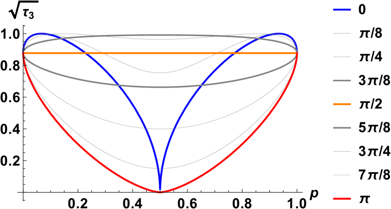
Figure 2: Characteristic curves for certain values of $\varphi=0$ (blue curve that interconnects concavely the points at $p=0,1$ with $(p,\sqrt{\tau_{3}})=(1/2,0)$) to the straight orange line at $\varphi=\pi/2$ up to $\varphi=\pi$ (the lowest red curve). The curves are symmetrically distributed around $\varphi=0$ and $\varphi=\pi$. The red lowest curve is the minimal characteristic curve and already convex. Therfore it constitutes a lower bound to $\widehat{\sqrt{\tau_{3}}}$. The zero polytope consists of a threefold degenerate zero at the angle $\varphi=\pi$ and a single zero at $\varphi=0$.

The pure states under consideration are hence

$$|\Psi(p,\varphi)\rangle:=\sqrt{pP_{1}}|\psi_{1}\rangle-\sqrt{(1-p)P_{2}}e^{i\varphi}|\psi_{2}\rangle\;.$$ (31)

In what follows, we will only consider the case $p_{3}=p_{4}=p_{5}=1/6$. This case implies $p_{rem}=1/2$ and the missing probabilities are $p_{1}(q)=(\cos^{2}\beta)/2=2q(1-q)$ and $p_{2}(q)=(\sin^{2}\beta)/2=(2q-1)^{2}/2$. Therefore the state $\Psi^{4}_{6;2}$ appears at the value of $1-q=(3+\sqrt{3})/6$ in the following diagrams. We obtain for the angle for this specific case $\alpha=-{\rm arctan}[\frac{\sqrt{2}}{3}]/2\approx-0.220255$.

Other values for the probabilities can be achieved by local $SL$-operations taking into consideration the invariance of the corresponding threetangle with respect to these operations. It must however be taken care that the normalization in general is not conserved.

The characteristic curves, hence the values of their absolute value for $\sqrt{\tau_{3}}$, are shown in Fig. 2 for various values of $\varphi$. We refer to Ref. Osterloh (2016a) to elucidate the procedure.

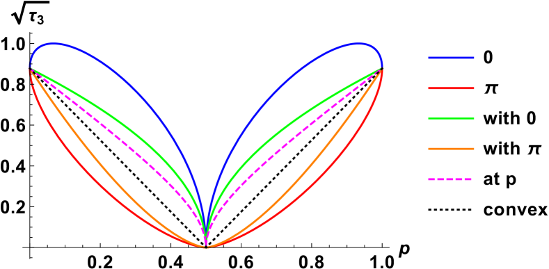
Figure 3: Upper bounds to the convex roof $\widehat{\sqrt{\tau_{3}}}$ of $\sqrt{\tau_{3}}$. The characteristic curves at the angles $\varphi=0,\pi$ are shown together with valid decompositions of the density matrix, namely a convex combination of a) one of the two eigenstates and $\rho_{0}=\frac{1}{2}(|\Psi(\frac{1}{2},0)\rangle\langle\Psi(\frac{1}{2},0)|+|\Psi(\frac{1}{2},\pi)\rangle\langle\Psi(\frac{1}{2},\pi)|)$ (black dotted lines) of the states taken from the zero-polytope $\Psi(\frac{1}{2},0)$ and $\Psi(\frac{1}{2},\pi)$, b) $|\Psi(p,0)\rangle\langle\Psi(p,0)|$ and $|\Psi(p,\pi)\rangle\langle\Psi(p,\pi)|$ (magenta dashed line), c) the state $|\Psi(\frac{1}{2},0)\rangle\langle\Psi(\frac{1}{2},0)|$ from the zero polytope and a state $|\Psi(q,\pi)\rangle\langle\Psi(q,\pi)|$ such that the line connecting both states intersects the center line of the bloch sphere at $(2p-1)$ (orange curve below the dotted line), d) the same as in c) but with $|\Psi(\frac{1}{2},\pi)\rangle\langle\Psi(\frac{1}{2},\pi)|$ from the zero-polytope and the corresponding state $|\Psi(q,0)\rangle\langle\Psi(q,0)|$ (green curve above the dashed and dotted line). The orange curve coincides with the convex roof.

Valid decompositions of the density matrix i.e. upper bounds to the convex roof $\widehat{\sqrt{\tau_{3}}}$ of $\sqrt{\tau_{3}}$ are visualized in Fig. (3). They show various convex combinations of $\rho$. The orange curve is given by the expression

$$\widehat{\sqrt{\tau_{3}}}[\rho_{1}(\frac{1}{2},p)]=\frac{2}{3^{3/4}}|2p-1|^{3/2}\;;$$ (32)

it coincides with the convex roof which we explain in what follows. For $p_{0}=(3\pm\sqrt{3})/6$ the convex-roof of $\rho_{0}:=\rho_{1}(1/2,p_{0})$ is $\widehat{\sqrt{\tau_{3}}}[\rho_{0}]=2/(3\sqrt{3})\approx 0.3849$.

As seen in Fig. 2, the characteristic curves are strictly concave around the single zero at $\varphi=0$ and $p=1/2$. This has two effects: a) any deviation of a decomposition-state around this value is greater than zero with a square-root behavior. And b) the weight of the states appears enhanced if more than one state is comprising the decomposition yielding a mixed state. For these two reasons one of the decomposition states is known to be the pure state which lies in the minimum of the single zero of the zero-polytope with concave behavior (linear behavior is included). One valid decomposition made of this decomposition state is the orange curve in Fig. 3. This acquires the absolute minimum because the characteristic curve at angle $\varphi=\pi$ is the minimal characteristic curve which is convex. Hence, any decomposition of pure states gives a resulting tangle which lies above that curve, similar to the argument in Lohmayer et al. (2006). More generally this is true for any homogeneous polynomial $SL$-invariant measure of entanglement of degree $2m$, if there exists a state which corresponds to a maximally $m$-fold degenerate solution in the zero-polytope that can be combined with the convexified minimal characteristic curve to give a decomposition of $\rho$, as is the case here. For a given density matrix $\rho$ the interconnecting straight lines with the minimal convexified characteristic curve hits the surface of the zero-polytope somewhere. A minimization of the effective entanglement measure along this decomposition of $\rho$ will give the convex roof. Due to convexity, it is enough minimizing along the curve on the surface of the zero-polytope that is facing the minimal characteristic curve on the bloch sphere.

It must be emphasized that also one of the upper bounds in Ref. Osterloh (2016b) was similar to this type except that the lowest convex curve was not convex; one should of course consider its convexification for reaching the convex roof. This should be reconsidered in the future.

If the zeros in the zero-polytope are not precisely at opposite angles of the sphere the optimal decomposition in the convex roof will change continuously from this absolutely optimal decomposition that we have in this case. It can therefor be considered as lower bound for this type of solutions and gives a better lower bound than the minimal characteristic curve as used in Refs. Eltschka and Siewert (2012a); Siewert and Eltschka (2012); Eltschka and Siewert (2014); Sentís et al. (2016) to lower bound the convex-roof making use of the symmetry in certain states.

We now briefly come back to the second case, in which the eigenstates can be directly read off Eq. (18). We have

$$\rho_{2}(\{p_{i}\};p)=pP_{1}|\psi_{1}\rangle\langle\psi_{1}|+(1-p)P_{2}|\psi_{2}\rangle\langle\psi_{2}|$$ (33)

where

$$|\psi_{1}\rangle = \sqrt{p_{1}}|111\rangle+\sqrt{p_{2}}e^{i\eta}|011\rangle+c_{3}|000\rangle\;,$$ (34)

$$|\psi_{2}\rangle = c_{4}|010\rangle+c_{5}|001\rangle\;,$$ (35)

and

$$P_{1} = p_{1}+p_{2}+p_{3}$$ (36)

$$P_{2} = p_{4}+p_{5}\;.$$ (37)

There is only one convex characteristic curve, which is the straight line connecting zero with $\sqrt{p_{1}p_{3}}/(p_{1}+p_{2}+p_{3})$. Hence

$$\widehat{\sqrt{\tau_{3}}}[\rho_{2}(\{p_{i}\};p)]=\frac{p\sqrt{p_{1}p_{3}}}{P_{1}}\;,$$ (38)

which means inserting $p=P_{1}$ for ${\rm tr}\;_{2}|\Psi^{4}_{6;2}\rangle\langle\Psi^{4}_{6;2}|$. For the same choice of probabilities as above we get $\widehat{\sqrt{\tau_{3}}}[\rho_{2}]=\frac{1}{3\sqrt{2}}\approx 0.2357$.

At the end, we briefly comment on the CKW inequality noting that for this particular state all concurrences do vanish. The extended inequality would however already be satisfied with $(\widehat{\sqrt{\tau_{3}}})^{2}$ as threetangleRegula et al. (2014, 2016a, 2016b).

To conclude, we have found states that, similar to the $W$-class which have all of their entanglement stored among two parties distributed all over the chain, do possess merely threetangle, again distributed all over the four parties. The states have the form $|\Psi^{4}_{6;2}\rangle$ (see Eq. (16)).

III.2.2 The state $|\Psi^{4}_{6;23}\rangle$

The state

$$|\Psi^{4}_{6;23}\rangle := \sqrt{p_{1}}|1111\rangle+$$

$$\sqrt{p_{2}}e^{i\eta}|0111\rangle+c_{3}|1011\rangle+c_{4}|0010\rangle+c_{5}|0001\rangle$$

with $c_{i}\in{\rm\kern 2.40005pt\vrule width=0.39993pt,height=6.28612pt,depth=-0.3014pt\kern-3.00003ptC}$, $i=2,\dots,5$, $|c_{i}|^{2}=p_{i}$, is normalized for $\sum_{i=1}^{5}p_{i}=1$. It is form-invariant with respect to permutation of the first and the last two qubits. Hence, there are also two essentially different reduced density matrices to be considered. They are

$${\rm tr}\;_{1}|\Psi^{4}_{6;23}\rangle\langle\Psi^{4}_{6;23}| = (\sqrt{p_{1}}|111\rangle+c_{3}|011\rangle)({\rm h.c.})$$

$$+(\sqrt{p_{2}}e^{i\eta}|111\rangle+c_{4}|010\rangle+c_{5}|001\rangle)({\rm h.c.})$$

$${\rm tr}\;_{3}|\Psi^{4}_{6;23}\rangle\langle\Psi^{4}_{6;23}| = p_{5}|001\rangle\langle 001|$$

$$+(\sqrt{p_{1}}|111\rangle+\sqrt{p_{2}}e^{i\eta}|011\rangle+c_{3}|101\rangle+c_{4}|000\rangle)({\rm h.c.})$$

The first reduced density matrix is written in subnormalized eigenvector form

$$\rho=|\psi_{1}\rangle\langle\psi_{1}|+|\psi_{2}\rangle\langle\psi_{2}|$$ (41)

whose subnormalized eigenvectors (obtained with the same method as in the preceding section) are

$$|\psi_{1}\rangle = \left(\sqrt{p_{1}}\cos\alpha-\sqrt{p_{2}}\sin\alpha\right)e^{i\eta}|111\rangle$$

$$+c_{3}e^{i\eta}\cos\alpha|011\rangle-\sin\alpha(c_{4}|010\rangle+c_{5}|001\rangle)$$

$$|\psi_{2}\rangle = \left(\sqrt{p_{1}}\sin\alpha+\sqrt{p_{2}}\cos\alpha\right)e^{i\eta}|111\rangle$$

$$+c_{3}e^{i\eta}\sin\alpha|011\rangle+\cos\alpha(c_{4}|010\rangle+c_{5}|001\rangle)$$

where

$$\tan 2\alpha = \frac{\sqrt{2p_{1}p_{2}}}{2(p_{1}+p_{3})-1}$$ (44)

$$\chi = \eta$$ (45)

and whose threetangle vanishes.

Only the second reduced density matrix

$$\rho_{3}=|\psi_{1}\rangle\langle\psi_{1}|+|\psi_{2}\rangle\langle\psi_{2}|$$ (46)

with

$$|\psi_{1}\rangle = \sqrt{p_{1}}|111\rangle+c_{4}|000\rangle+$$

$$\qquad\sqrt{p_{2}}e^{i\eta}|011\rangle+c_{3}|101\rangle$$

$$|\psi_{2}\rangle = \sqrt{p_{5}}|001\rangle$$ (48)

has nontrivial threetangle. Its zero-simplex consists of a single point at the end of the interval $[0,1]$ which goes back to a fourfold-degenerate root. It leads consequently to a single linear characteristic curve. Therefore the convex roof of

$$\rho(\{p_{i}\};p):=\frac{p}{1-p_{5}}|\psi_{1}\rangle\langle\psi_{1}|+\frac{1-p}{p_{5}}|\psi_{2}\rangle\langle\psi_{2}|$$ (49)

equals

$$\widehat{\sqrt{\tau_{3}}}[\rho(\{p_{i}\};p)]=p\frac{\sqrt{p_{1}p_{4}}}{(1-p_{5})}\;,$$ (50)

so that we obtain

$$\widehat{\sqrt{\tau_{3}}}[\rho_{3}]=\sqrt{p_{1}p_{4}}\;.$$ (51)

These states however have always a non-vanishing concurrence $C[\rho_{ij}]=\sqrt{2p_{\!{}_{J_{i}}}p_{\!{}_{J_{j}}}}$ and $\vec{J}=(3,2,5,4)$ for non-vanishing $p_{k}$, $k=2,\dots,5$. However, an extended monogamy inequality would be satisfied with $\widehat{\sqrt{\tau_{3}}}^{2}$ as threetangle, as before.

III.3 States derived from $\Psi^{4}_{4}$

As we come to the states derived from $\Psi^{4}_{4}$ there are two cases to be considered left. Inserting the weights for the state (8) we obtain

$$|\Psi^{4}_{4;1}\rangle = \sqrt{p_{1}}|0000\rangle+c_{2}|1100\rangle+c_{3}|0010\rangle+$$ (52)

$$\quad\sqrt{p_{4}}e^{i\eta}|0001\rangle$$

where the $c_{i}$ are complex, $|c_{i}|^{2}=p_{i}$, and which is normalized if $\sum_{i=1}^{4}p_{i}=1$. This state is form-invariant under permutations of the first and last two qubits, and hence only two different reduced density matrices exist. They consist of two states which have no three-tangled state in their range.

The second state has the same form-invariance as above. It is

$$|\Psi^{4}_{4;2}\rangle = c_{1}|1111\rangle+\sqrt{p_{2}}|0011\rangle+\sqrt{p_{3}}e^{i\eta}|0010\rangle+$$ (53)

$$\quad c_{4}|0001\rangle$$

So there are only two essentially different reduced density matrices

$${\rm tr}\;_{1}|\Psi^{4}_{4;2}\rangle\langle\Psi^{4}_{4;2}| = p_{1}|111\rangle\langle 111|+$$

$$(\sqrt{p_{2}}|011\rangle+\sqrt{p_{3}}e^{i\eta}|010\rangle+c_{4}|001\rangle)({\rm h.c.})$$

$${\rm tr}\;_{4}|\Psi^{4}_{4;2}\rangle\langle\Psi^{4}_{4;2}| = p_{3}|001\rangle\langle 001|+$$

$$(c_{1}|111\rangle+\sqrt{p_{2}}|001\rangle+c_{4}|000\rangle)({\rm h.c.})$$

Whereas the first density matrix has no threetangled state in its range, the eigenstates of ${\rm tr}\;_{4}|\Psi^{4}_{4;2}\rangle\langle\Psi^{4}_{4;2}|$ are

$$|\psi_{1}\rangle \propto \cos\alpha\left(c_{1}|111\rangle+c_{4}|000\rangle\right)$$

$$+(\sqrt{p_{2}}\cos\alpha-\sqrt{p_{3}}e^{2i\eta}\sin\alpha)|001\rangle$$

$$|\psi_{2}\rangle \propto \sin\alpha\left(c_{1}|111\rangle+c_{4}|000\rangle\right)$$

$$+(\sqrt{p_{2}}\sin\alpha+\sqrt{p_{3}}e^{2i\eta}\cos\alpha)|001\rangle$$

with the condition for orthogonality of the two vectors being

$$\tan(2\alpha) = \frac{\sqrt{p_{2}p_{3}}}{2(2p_{3}-1)}$$ (58)

$$\chi = -\eta$$ (59)

The weights of the normalized eigenfunctions are

$$P_{1}=\cos^{2}\alpha-p_{3}\cos(2\alpha)-\sqrt{p_{1}p_{3}}\sin(2\alpha)\cos(2\eta)$$ (60)

$$P_{2}=\sin^{2}\alpha+p_{3}\cos(2\alpha)+\sqrt{p_{1}p_{3}}\sin(2\alpha)\cos(2\eta)$$ (61)

respectively. This state has a four-fold solution for the vanishing of the threetangle. They to a zero-polytope which is consisted of a single point in ${\rm\kern 2.40005pt\vrule width=0.39993pt,height=6.28612pt,depth=-0.3014pt\kern-3.00003ptC}$ corresponding to a single state whose threetangle vanishes. The convex roof is known exactly for this situationRegula and Adesso (2016). It is independent of the decomposition of the density matrix, hence it is a linear function connecting the threetangles of the eigenvectors, which are

$$\sqrt{\tau_{3}}[\psi_{1}] = \frac{\cos^{2}(\alpha)\,\sqrt{p_{1}p_{4}}}{P_{1}}$$ (62)

$$\sqrt{\tau_{3}}[\psi_{2}] = \frac{\sin^{2}(\alpha)\,\sqrt{p_{1}p_{4}}}{P_{2}}\;.$$ (63)

This results in

$$\widehat{\sqrt{\tau_{3}}}[{\rm tr}\;_{4}|\Psi^{4}_{4;2}\rangle\langle\Psi^{4}_{4;2}|]=\sqrt{p_{1}p_{4}}\;.$$ (64)

The remaining state is

$$|\Psi^{4}_{4;4}\rangle = \sqrt{p_{1}}|1111\rangle+c_{2}|1100\rangle+c_{3}|0010\rangle+$$ (65)

$$\quad\sqrt{p_{4}}e^{i\eta}|1110\rangle$$

where $c_{i}\in{\rm\kern 2.40005pt\vrule width=0.39993pt,height=6.28612pt,depth=-0.3014pt\kern-3.00003ptC}$, $|c_{i}|^{2}=p_{i}$ and with the same condition $\sum_{i=1}^{4}p_{i}=1$ for normalization. This state possesses form-invariance with respect to the first two qubits only. The reduced density matrices are

$${\rm tr}\;_{1}|\Psi^{4}_{4;4}\rangle\langle\Psi^{4}_{4;4}| = p_{2}|010\rangle\langle 010|+$$

$$(\sqrt{p_{1}}|111\rangle+c_{2}|100\rangle+\sqrt{p_{4}}e^{i\eta}|110\rangle)({\rm h.c.})$$

$${\rm tr}\;_{3}|\Psi^{4}_{4;4}\rangle\langle\Psi^{4}_{4;4}| = p_{2}|010\rangle\langle 010|+$$

$$(\sqrt{p_{1}}|111\rangle+c_{3}|000\rangle+\sqrt{p_{4}}e^{i\eta}|110\rangle)({\rm h.c.})$$

$${\rm tr}\;_{4}|\Psi^{4}_{4;4}\rangle\langle\Psi^{4}_{4;4}| = p_{1}|111\rangle\langle 111|+$$

$$(c_{2}|110\rangle+c_{3}|001\rangle+\sqrt{p_{4}}e^{i\eta}|111\rangle)({\rm h.c.})$$

The first state has no threetangled state in its whole range; only tracing out the third, or the fourth qubit renders a non-zero contribution.

Tracing out the third qubit leads directly to the eigenvectors $\psi_{2}=|010\rangle$ and $\psi_{1}\propto\sqrt{p_{1}}|111\rangle+c_{3}|000\rangle+\sqrt{p_{4}}e^{i\eta}|110\rangle$ with corresponding eigenvalues $p_{2}$ and $1-p_{2}$, respectively. As above the convex roof is known exactly to be the linear interpolation between the eigenstates of $\rho$; hence between zero and

$$\sqrt{\tau_{3}}[\psi_{1}]=\frac{\sqrt{p_{1}p_{3}}}{1-p_{2}}\;.$$ (69)

Here again, this is trivially seen because the characteristic curves all coincide with a straight line which is hence identical with the lowest characteristic curve which is already convex. Hence, this corresponds to a unique four-fold solution of the zero-polytopeRegula and Adesso (2016).

Tracing out the fourth qubit gives the eigenstates

$$|\psi_{1}\rangle \propto (\sqrt{p_{1}}\sin\alpha+\sqrt{p_{4}}\cos\alpha)|111\rangle$$ (70)

$$+e^{i\eta}\cos\alpha(c_{2}|110\rangle+c_{3}|001\rangle)$$

$$|\psi_{2}\rangle \propto (\sqrt{p_{1}}\cos\alpha-\sqrt{p_{4}}\sin\alpha)|111\rangle$$ (71)

$$-e^{i\eta}\sin\alpha(c_{2}|110\rangle+c_{3}|001\rangle)$$

where

$$\tan(2\alpha) = \frac{2\sqrt{p_{1}p_{4}}}{1-2p_{1}}\;,$$ (72)

$$\chi = \eta\;.$$ (73)

The modulus squared of the eigenstates are

$$P_{1} = \sin^{2}\alpha+p_{1}\cos(2\alpha)-\sin(2\alpha)\sqrt{p_{1}p_{4}}\;,$$ (74)

$$P_{2} = \cos^{2}\alpha-p_{1}\cos(2\alpha)+\sin(2\alpha)\sqrt{p_{1}p_{4}}\;.$$ (75)

The convex roof for the threetangle linearly connects the tangles of the eigenstatesRegula and Adesso (2016)

$$\sqrt{\tau_{3}}[\psi_{1}] = \frac{\cos^{2}(\alpha)\,\sqrt{p_{2}p_{3}}}{P_{1}}\;,$$ (76)

$$\sqrt{\tau_{3}}[\psi_{2}] = \frac{\sin^{2}(\alpha)\,\sqrt{p_{2}p_{3}}}{P_{2}}\;.$$ (77)

The only non-zero concurrences are $C[\rho_{1,2}]=\sqrt{2p_{3}p_{4}}$ and $C[\rho_{3,4}]=\sqrt{2p_{1}p_{2}}$, where $\rho_{i,j}$ is the reduced density matrix of qubits $i$ and $j$. We state that whenever all the concurrences vanish, also all the threetangles are zero. We therefor have no perfect analogy to the $W$ states.

Hence, states derived from $\Psi^{4}_{4}$ do never lead to a perfect analogue of the $W$-class. In all cases the derived states do satisfy an extended monogamy relation with $\widehat{\sqrt{\tau_{3}}}^{2}$ inserted as threetangle.

IV Conclusions

In conclusion we have singled out states for four qubits that, different from the states from the $W$-class that contain two-tangle, contain only threetangle which however is globally distributed. To this end we have analyzed specific four-qubit states which are located in the $SL$ null-cone: this guarantees that all possible $SL$-invariant four-tangles are zero. For having states like this, we apply partial spin flips to a c-balanced stateJohansson et al. (2014). All states satisfy an extended monogamy relation with $\widehat{\sqrt{\tau_{3}}}^{2}$ inserted as threetangle. It has however already been excluded that an extension of this kind might existRegula et al. (2016b). Since the value of the threetangle will shrinkOsterloh (2016b) (see also Ref. Eltschka et al. (2009)) with growing $q$ in $\widehat{\sqrt[q]{\tau_{3}}}^{q}$, the result will finally be upper bounded by $q=2$.
It will be of interest if the various threetangles can be rendered equal. The latter could be achieved by locally applying $SL$ operations to the states, making use of $SL$-invariants which scale quadratically in $\psi$ (or linearly in $\rho$) Viehmann et al. (2011, 2012). Also would it be intriguing if such states exist for larger number of qubits $q$ and $n$-site entanglement. However, for growing number of qubits, the considered reduced density matrices usually are of higher rank. It would be nice to see whether translationally (or even permutationally) invariant versions of such states will exist and whether it is possible to write such a state for arbitrary number of qubits as for the $W$ state. It is however clear that the permutationally extended version of the state $|\Psi^{4}_{6;2}\rangle$ with real coefficients will always carry four-tangle unless it becomes a state in the $W$-class for $p_{2}=0$.

As an interesting byproduct it is demonstrated that the exact convex roof is achieved for the rank-two case of a homogeneous degree $2m$ polynomial $SL$-invariant measure of entanglement, if there are states which correspond to a maximally $m$-fold degenerate solution in the zero-polytope that can be combined with the convexified minimal characteristic curve to give a decomposition of $\rho$. One has to take the minimum of the results, if more than one such state does exist. The threetangle has homogeneous degree 4, hence $m=2$ for this case. The minimum over thus constructed decomposition states represents a lower bound to the $SL$-invariant entanglement measure under consideration; it is of course larger than the lowest characteristic curve used in Refs. Eltschka and Siewert (2012a); Siewert and Eltschka (2012); Eltschka and Siewert (2012b); Eltschka and Siewert (2013).

We consider it worth to hint towards the alternating signs appearing in the monogamy equality of Ref. Eltschka and Siewert (2015). It could therefore be that a full analogue to the $W$ state may appear only for an even number of $n$. In order to test this, one should at least analyze corresponding states for five qubits.
This alternating sum also appears elsewhere: for representations of the univeral state inversionEltschka and Siewert (2017) and in the shadow inequalitiesHuber et al. (2017). Here merge apparently very different fields as multipartite entanglement and quantum error correcting codes. Also the Gell-Mann representatives for the operator $\sigma_{y}$ for qubits emerging from the representation of the general state inversionEltschka and Siewert (2017) have also appeared before inside the operator with full $SL(d)$ symmetryOsterloh (2015) that creates the determinant and is used to form the $SL$-invariant analogue to the concurrence for qubits.

References

• Coffman et al. (2000) V. Coffman, J. Kundu, and W. K. Wootters, Phys. Rev. A 61, 052306 (2000).
• Osborne and Verstraete (2006) T. J. Osborne and F. Verstraete, Phys. Rev. Lett. 96, 220503 (2006).
• Dür et al. (2000) W. Dür, G. Vidal, and J. I. Cirac, Phys. Rev. A 62, 062314 (2000).
• Johansson et al. (2014) M. Johansson, M. Ericsson, E. Sjöqvist, and A. Osterloh, Phys. Rev. A 89, 012320 (2014).
• Osterloh and Siewert (2006) A. Osterloh and J. Siewert, Int. J. Quant. Inf. 4, 531 (2006).
• Osterloh and Siewert (2010) A. Osterloh and J. Siewert, New J. Phys. 12, 075025 (2010).
• Luque et al. (2007) J.-G. Luque, J.-Y. Thibon, and F. Toumazet, Math. Struct. Comp. Sc. 1133 (2007).
• Johansson et al. (2012) M. Johansson, M. Ericsson, K. Singh, E. Sjöqvist, and M. S. Williamson, Phys. Rev. A 85, 032112 (2012).
• Osterloh and Siewert (2005) A. Osterloh and J. Siewert, Phys. Rev. A 72, 012337 (2005).
• Doković and Osterloh (2009) D. Ž.  Doković and A. Osterloh, J. Math. Phys. 50, 033509 (2009).
• Viehmann et al. (2011) O. Viehmann, C. Eltschka, and J. Siewert, Phys. Rev. A 83 (2011).
• Osterloh (2016a) A. Osterloh, Phys. Rev. A 94, 062333 (2016a).
• Lohmayer et al. (2006) R. Lohmayer, A. Osterloh, J. Siewert, and A. Uhlmann, Phys. Rev. Lett. 97, 260502 (2006).
• Osterloh (2016b) A. Osterloh, Phys. Rev. A 94, 012323 (2016b).
• Eltschka and Siewert (2012a) C. Eltschka and J. Siewert, Phys. Rev. Lett. 108, 020502 (2012a).
• Siewert and Eltschka (2012) J. Siewert and C. Eltschka, Phys. Rev. Lett. 108, 230502 (2012).
• Eltschka and Siewert (2014) C. Eltschka and J. Siewert, Phys. Rev. A 89, 022312 (2014).
• Sentís et al. (2016) G. Sentís, C. Eltschka, and J. Siewert, Phys. Rev. A 94, 020302(R) (2016).
• Regula et al. (2014) B. Regula, S. Di Martino, S. Lee, and G. Adesso, Phys. Rev. Lett. 113, 110501 (2014).
• Regula et al. (2016a) B. Regula, S. Di Martino, S. Lee, and G. Adesso, Phys. Rev. Lett. 116, 049902(E) (2016a).
• Regula et al. (2016b) B. Regula, A. Osterloh, and G. Adesso, Phys. Rev. A 93, 052338 (2016b).
• Regula and Adesso (2016) B. Regula and G. Adesso, Phys. Rev. Lett. 116, 070504 (2016).
• Eltschka et al. (2009) C. Eltschka, A. Osterloh, and J. Siewert, Phys. Rev. A 80, 032313 (2009).
• Viehmann et al. (2012) O. Viehmann, C. Eltschka, and J. Siewert, Appl. Phys. B 106, 533 (2012), spring Meeting of the German-Physical-Society, Dresden, GERMANY, 2011.
• Eltschka and Siewert (2012b) C. Eltschka and J. Siewert, Sci. Rep. 2, 942 (2012b).
• Eltschka and Siewert (2013) C. Eltschka and J. Siewert, Quant. Inf. Comp. 13, 210 (2013).
• Eltschka and Siewert (2015) C. Eltschka and J. Siewert, Phys. Rev. Lett. 114, 140402 (2015).
• Eltschka and Siewert (2017) C. Eltschka and J. Siewert (2017), arXiv:1708.09639.
• Huber et al. (2017) F. Huber, C. Eltschka, J. Siewert, and O. Gühne (2017), arXiv:1708.06298.
• Osterloh (2015) A. Osterloh, J. Phys. A 48, 065303 (2015).