Neutron Electric Dipole Moment on the Lattice

Abstract

For the neutron to have an electric dipole moment (EDM), the theory of nature must have T, or equivalently CP, violation. Neutron EDM is a very good probe of novel CP violation in beyond the standard model physics. To leverage the connection between measured neutron EDM and novel mechanism of CP violation, one requires the calculation of matrix elements for CP violating operators, for which lattice QCD provides a first principle method. In this paper, we review the status of recent lattice QCD calculations of the contributions of the QCD $\Theta$-term, the quark EDM term, and the quark chromo-EDM term to the neutron EDM.

1 Introduction

Electric dipole moment (EDM) of the neutron measures the separation of positive and negative charge in the neutron and is necessarily aligned along the spin axis. For a neutron to have an EDM, the theory of elementary particles must violate parity (P) and time reversal (T) invariance, and charge conjugation and parity (CP) symmetry if CPT is conserved. Under a parity transformation, the EDM of any particle changes its sign while the direction of the spin remains the same. Under time-reversal transformation, the spin flips its direction while the EDM stays unchanged.

So far, a nonvanishing neutron EDM (nEDM) has not been observed, and the current experimental upper bound is $3.0\times 10^{-26}e{\cdot}\textrm{cm}$ Afach:2015sja . In recent experiments, the nEDM is measured by the change in the spin precession frequency of ultracold-neutrons aligned in a magnetic field under a flip in the direction of a strong background electric field. Figure 1 shows the history of the experimental upper bound on the neutron EDM, as well as the target precision, $\sim 5\times 10^{-28}e{\cdot}\textrm{cm}$ psi ; Picker:2016ygp ; fermII ; sns ; CryoEDM , of proposed experiments.

In the standard model, the leading contribution to nEDM due to the CP violating phase in the CKM matrix comes from three-loop and higher order diagrams, and the expected size is more than 5 orders of magnitude below the current experimental bound Dar:2000tn . In extensions of the standard models, however, nEDM can appear at one-loop due to novel CP violating interactions. In some of the most popular models, such as supersymmetric (SUSY) models, the expected size of the nEDM is between $10^{-25}$–$10^{-28}$$e{\cdot}\textrm{cm}$ as shown in Figure 1. Therefore, a nEDM smaller that $10^{-28}$$e{\cdot}\textrm{cm}$ will put a serious constraint on those models Pospelov:2005pr ; RamseyMusolf:2006vr ; Engel:2013lsa .

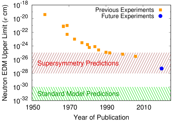
Figure 1: The timeline of the upper bound on the neutron EDM from previous and future experiments. The yellow squares are the previous bounds, and the blue dot is the sensitivity target of next generation experiments. In the standard model, the leading contribution to nEDM from the CP violating phase in the CKM matrix arises at three-loops, and the expected size of nEDM is more than 5 orders of magnitude below the current experimental bound, as shown by the green shaded area in the plot Dar:2000tn . In extensions of the standard models, however, nEDM can appear at one-loop with the new CP violating interactions. In some of the most popular models, such as SUSY, the expected size of nEDM covers the regions of the current and future experimental bound, as shown by the red shaded area Pospelov:2005pr ; RamseyMusolf:2006vr ; Engel:2013lsa .

There are two main outcomes of neutron EDM experiments for BSM physics. First, a non-zero measurement of nEDM would establish new sources of CP violation, which is one of Sakharov’s three conditions for weak-scale baryogenesis Sakharov:1967dj . The CP violation in the standard model is not sufficient to explain observed the baryon asymmetry of the universe, and it requires new sources of CP violation from beyond the standard model (BSM) Bernreuther:2002uj . Neutron EDM is a good probe for such novel CP violation. Second, most BSM theories have additional sources of CP violation. There are many BSM scenarios predicting a nEDM between $10^{-25}$ – $10^{-28}e{\cdot}\textrm{cm}$, and upcoming experiments will put constraints on them psi ; Picker:2016ygp ; fermII ; sns ; CryoEDM . This requires both the measurement of, or a bound on, the neutron EDM, and the calculations of the matrix elements of novel CP violating operators within the neutron states. Current non-lattice estimates of the matrix elements have large uncertainties Engel:2013lsa . Lattice QCD can provide a first principle, non-perturbative method for calculating these matrix elements.

To analyze novel CP violation, we work within the framework of effective field theories and classify operators by their canonical dimension Pospelov:1999mv . At hadronic scale, the effective Lagrangian for the CP violating interactions at dimension 4, 5 and 6 can be written as

$$\mathcal{L}_{\text{CPV}}^{d=4,5,6}= -\frac{\mathrm{g}^{2}}{32\pi^{2}}{\theta}G{\widetilde{G}}-\frac{i}{2}\sum_{q=u,d,s}d_{q}\bar{q}(\sigma_{\mu\nu}F^{\mu\nu})\gamma_{5}q-\frac{i}{2}\sum_{q=u,d,s}\tilde{d}_{q}\bar{q}(\sigma_{\mu\nu}G^{\mu\nu})\gamma_{5}q$$

$$+d_{w}\frac{\mathrm{g}}{6}f^{abc}G^{a}_{\mu\nu}{\widetilde{G}}^{\nu\rho,b}G_{\rho}^{\mu,c}+\sum_{i}C_{i}^{(4q)}O_{i}^{(4q)}\,,$$ (1)

where $\mathrm{g}$ is the QCD coupling constant, and ${\widetilde{G}}^{\mu\nu,b}=\varepsilon^{\mu\nu\alpha\beta}G^{b}_{\alpha\beta}/2$. The first term on the right hand side (r.h.s) is the dimension-4 $\Theta$-term already allowed in QCD, and the next two terms are the dimension-5 quark EDM (qEDM) and quark chromo-EDM (cEDM) terms. There are two types of dimension-6 terms in the second line in the above equation: the Weinberg three-gluon operator and various four-quark operators.

If the matrix elements of all the operators are $O(1)$ and the anomalous dimensions are small, then the $\mathcal{O}(1/\Lambda_{\rm scale}^{D-4})$ suppression implies that the lower mass dimension operators are more important. However, it turns out that the current bound on the nEDM already makes the dimension-4 QCD $\Theta$-term unnaturally tiny; $\bar{\theta}\leq\mathcal{O}(10^{-9}-10^{-11})$ Crewther:1979pi ; Abada:1990bj ; Pospelov:1999mv ; Mereghetti:2010kp , where $\bar{\theta}$ is the total effective CP violating angle $\bar{\theta}=\theta+\arg\det M_{\textrm{CKM}}$ with the quark mixing matrix $M_{\textrm{CKM}}$ . The unexpected smallness of this number is known as the strong CP problem. One of the popular models explaining the strong CP problem is the Peccei-Quinn mechanism Peccei:1977hh ; Peccei:1977ur , which requires the existence of the, as yet unobserved, axion. The two dimension-5 operators typically arise at the TeV scale as dimension-6 operators involving a Higgs. At the hadronic scale, 1 GeV, the Higgs fields are replaced by its vacuum expectation value, $v_{\mathrm{EM}}$, and the operator becomes dimension-5 with the coefficients suppressed by $v_{\mathrm{EM}}/M_{\mathrm{BSM}}^{2}$. How well these dimensional arguments work and which terms in Eq. (1) make the largest contribution to nEDM depends on the details of the BSM theory. But, while the couplings depend on the starting BSM model, the matrix elements of these operators within the neutron states are model independent results. Thus, lattice QCD calculation of the matrix elements of these operators will play an important role in connecting the measured neutron EDM and novel CP violation in BSM scenarios, i.e., knowing the matrix elements along with the bound on (or the value of) the nEDM, one can put bounds on the couplings and thus on the parameter space of allowed BSM theories.

In this paper, we review recent progress in Lattice QCD calculations of the matrix elements of these CP violating operators. We start by discussing the contribution of the QCD $\Theta$-term to the nEDM and use it to illustrate the various methods used in the calculations.

2 QCD $\Theta$-term

There are three strategies for the calculation of the contribution of CP violating operators to the neutron EDM on the lattice. We illustrate these three approaches for the case of the CP-violating $\Theta$-term whose volume integral is the topological charge $Q_{\mathrm{top}}$. They are the external electric field method Aoki:1989rx ; Aoki:1990ix ; Shintani:2006xr ; Shintani:2008nt , expansion in ${{\theta}}$ Shintani:2005xg ; Berruto:2005hg ; Shindler:2015aqa ; Alexandrou:2015spa ; Shintani:2015vsx , and simulation with imaginary ${{\theta}}$ Izubuchi:2008mu ; Aoki:2008gv ; Guo:2015tla .

2.1 External Electric Field Method

The first method uses an external electric field Aoki:1989rx ; Aoki:1990ix ; Shintani:2006xr ; Shintani:2008nt , in which the neutron EDM, $d_{N}$, is extracted from the energy difference of the neutron states with spin $\vec{S}$ aligned [anti]parallel to the external electric field $\vec{\mathcal{E}}$:

$$E^{{\theta}}_{\vec{S}}-E^{{\theta}}_{-\vec{S}}\approx 2d_{N}{{\theta}}\vec{S}\cdot\vec{\mathcal{E}}\,.$$ (2)

For a given value of ${{\theta}}$, the effect of the $\Theta$-term is included by reweighting the nucleon correlation function with the topological charge:

$$\big{\langle}N\bar{N}\big{\rangle}_{{\theta}}(\vec{\mathcal{E}},t)=\big{\langle}N(t)\bar{N}(0)e^{i{{\theta}}Q_{\mathrm{top}}}\big{\rangle}_{\vec{\mathcal{E}}}\,,$$ (3)

where the expectation value on the r.h.s is evaluated on lattice configurations generated without the $\Theta$-term. This method extracts the neutron EDM from a spectral quantity, not the form factor $F_{3}$ as discussed next, so the results are not affected by the mixing under parity violation problem discussed in Section 3.

2.2 Expansion in ${{\theta}}$

Based on the current experimental bound of the neutron EDM and model studies, we know that the coupling ${\theta}$ is tiny. Hence it can be treated as a small expansion parameter. Any expectation value in presence of a small QCD $\Theta$-term can then be written as follows Shintani:2005xg ; Berruto:2005hg ; Shindler:2015aqa ; Alexandrou:2015spa ; Shintani:2015vsx :

$$\big{\langle}O(x)\big{\rangle}_{{\theta}} =\frac{1}{Z_{{\theta}}}\int d[U,q,\bar{q}]O(x)e^{-S_{QCD}+i{{\theta}}Q_{\mathrm{top}}}$$

$$=\big{\langle}O(x)\big{\rangle}_{{{\theta}}=0}+i{{\theta}}\big{\langle}O(x)Q_{\mathrm{top}}\big{\rangle}_{{{\theta}}=0}+O({{\theta}}^{2})\,.$$ (4)

In the second line of the above equation, the QCD $\Theta$-term effect is included at the lowest order by measuring the correlation of the topological charge with the observable $O$, using configurations generated without the $\Theta$-term.

To calculate the nEDM, the operator $O$ is chosen as the matrix element of the vector current within the neutron states. Assuming PT invariance, the matrix element, calculated as a function of $q_{\mu}$, the momentum transfered by the vector current, can be decomposed in terms of Lorentz covariant form factors:

$$\langle NV_{\mu}N\rangle_{{\theta}}=\bar{u}\left[F_{1}(q^{2})\gamma_{\mu}+i\frac{F_{2}(q^{2})}{2m_{N}}\sigma_{\mu\nu}q^{\nu}-\frac{F_{3}(q^{2})}{2m_{N}}\sigma_{\mu\nu}q^{\nu}\gamma_{5}\right]u\,.$$ (5)

Of these, the form factor of interest is $F_{3}$ at zero-momentum transfer. This is extracted by extrapolating $F_{3}(q^{2})$, measured at finite $q^{2}$, because the term containing $F_{3}$ only contributes at $q^{\nu}\neq 0$ as can be seen from Eq. (5). Then the contribution to $d_{N}$ is given by

$$d_{N}=\lim_{q^{2}\rightarrow 0}\frac{F_{3}(q^{2})}{2m_{N}}\,.$$ (6)

This approach, which relies on calculating the form-factor $F_{3}$ from nucleon matrix elements, requires a careful handling of the neutron spinors in a theory with P violation. Most previous calculations did not correctly account for this subtlety Abramczyk:2017oxr . The problem can be corrected retroactively, and in Figure 3 we show the resulting reduction in the value reported in recent calculations Alexandrou:2015spa ; Shintani:2015vsx ).

2.3 Imaginary ${{\theta}}$ Simulation

The $\Theta$-term in Euclidean space-time is purely imaginary, and Monte Carlo simulations including the $\Theta$-term face the sign problem. One way to circumvent this issue is to make the action real by taking ${{\theta}}$ to be purely imaginary Izubuchi:2008mu ; Aoki:2008gv ; Guo:2015tla . Assuming that the theory is analytic around ${{\theta}}=0$, the results can then be continued to real ${{\theta}}$ for small ${{\theta}}$. Furthermore, this calculation can be carried out using the axial anomaly whereby the QCD $\Theta$-term is chirally rotated to the fermionic term $S_{{\theta}}^{q}$ as

$${{\theta}}\to i\tilde{{{\theta}}},\qquad S_{{\theta}}^{q}=\tilde{{{\theta}}}\frac{m_{l}m_{s}}{2m_{s}+m_{l}}\sum_{x}\bar{q}(x)\gamma_{5}q(x)\,.$$ (7)

Lattice simulation can then be performed by adding $S_{{\theta}}^{q}$ to the original QCD action. In this approach, the EDM is again extracted from the form factor analysis, so the results are affected by the mixing induced by parity violation discussed in Section 3. Again, in Figure 3 we show one of the recent results Guo:2015tla with and without the correction due to this mixing problem.

2.4 Variance Reduction using Cluster Decomposition

In the calculation of neutron EDM induced by the QCD $\Theta$-term using ${{\theta}}$-expansion or external electric field method, one needs to calculate correlators reweighted by the topological charge. Recently, the authors of Ref. Liu:2017man reported an error reduction technique using cluster decomposition. The main idea is to calculate the topological charge only in the vicinity of the sink in the momentum projection summation. Let us consider a neutron two-point correlator reweighted with the topological charge $Q$:

$$C_{R}(t) =\left\langle\sum_{x}N(\vec{x},t)\bar{N}(\mathcal{G},0)Q_{R}(x)\right\rangle,$$

$$Q_{R}(x) =\sum_{||x-y||<R}q(y)\,,$$ (8)

where $\mathcal{G}$ is the source grid. In conventional calculations, $Q$ is calculated by summing the topological charge density $q(y)$ from all lattice points. In the new formula, however, the topological charge is calculated only up to a certain radius $R$ from the sink point under the assumption that correlations due to long-distance points are negligible.

Figure 2 presents the CP violating phase, labeled $\alpha^{1}$ and calculated using the Eq. (8), as a function of the cutoff radius $R$. Data show that the mean value of $\alpha^{1}$ saturates at some reasonably small value of $R$. Including the contributions of the topological density from larger $R$ only increases the statistical noise. Considering that the mean value still exhibits significant fluctuations, a more detailed cost-benefit analysis of the approximation is required.

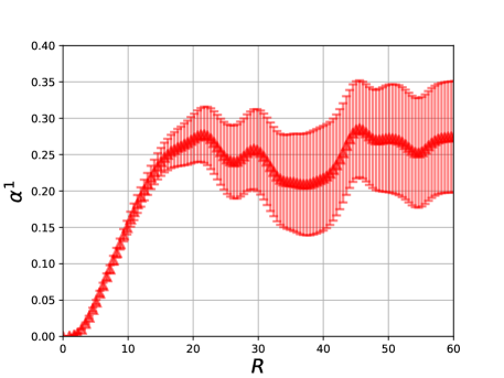
Figure 2: CP violating phase $\alpha$ (denoted as $\alpha^{1}$ in the figure) as a function of the cutoff radius $R$ presented in Ref. Liu:2017man . The central value of the $\alpha$ appears to saturate after $R$ is larger than about 15 lattice spacings, which corresponds to 1.71 fm in physical unit, while the statistical error grows as $R$ is increased.

3 Extracting $F_{3}$ in a Theory with Parity Violation

In a theory with P and CP symmetry, the spinor $u$ of the neutron state satisfies the following Dirac equation:

$$\left(ip_{\mu}\gamma_{\mu}+m\right)u=0\,,$$ (9)

with $\gamma_{4}$ the parity operator: $u_{\vec{p}}\rightarrow\gamma_{4}u_{-\vec{p}}$ under P. When CP, but not PT, is violated, the Dirac equation is only modified by a phase factor to

$$\left(ip_{\mu}\gamma_{\mu}+me^{-2i\alpha\gamma_{5}}\right)\tilde{u}=0\,,$$ (10)

where the spinor that solves the modified equation is defined to be $\tilde{u}$. Furthermore, for this equation, $\gamma_{4}$ is no longer the parity operator, rather under parity $\tilde{u}_{\vec{p}}\rightarrow e^{-2i\alpha\gamma_{5}}\gamma_{4}\tilde{u}_{-\vec{p}}$. The two solutions $u$ and $\tilde{u}$ are related as

$$\tilde{u}=e^{i\alpha\gamma_{5}}u,\qquad\bar{\tilde{u}}=\bar{u}e^{i\alpha\gamma_{5}}.$$ (11)

When calculating the form factors $F_{2}$ and $F_{3}$, it is important to enforce that $F_{2}$ is the parity-even magnetic form factor while $F_{3}$ is the P and CP odd electric form factor. There are two ways to enforce these symmetry requirements. The first is to properly include the phase defined in Eq. (11) in the definition of the matrix element. In that case the decomposition into the form factors is the same as in a theory with CP symmetry with unmodified spinors $u$. Alternatively, one can calculate the standard matrix element, and then undo the mixing between $F_{2}$ and $F_{3}$ due to the non-standard parity transformation with phase $\alpha$. Then, the two form factors $F_{2}$ and $F_{3}$ are given in terms of $\tilde{F}_{2}$ and $\tilde{F}_{3}$ as in Eq. (14).

In both cases, the phase $\alpha$ has to be extracted from the nucleon 2-point function. In this extraction, it is important to note that the phase $\alpha$ is state dependent. In Section 5, we show that the $\alpha$ corresponding to the ground state is given by the long-time behavior of the nucleon 2-point function, i.e., when the ground state dominates.

In the first approach, one includes the phase in the calculation of the n-point functions:

$$e^{-i\alpha\gamma_{5}}\langle\tilde{N}V_{\mu}\bar{\tilde{N}}\rangle e^{-i\alpha\gamma_{5}}=\langle NV_{\mu}\bar{N}\rangle,\qquad e^{-i\alpha\gamma_{5}}\langle\tilde{N}\bar{\tilde{N}}\rangle e^{-i\alpha\gamma_{5}}=\langle N\bar{N}\rangle$$

$$\Longrightarrow\quad\bar{u}\left(F_{1}(q^{2})\gamma_{\mu}+i\frac{[\gamma_{\mu},\gamma_{\nu}]}{2}q_{\nu}\frac{F_{2}(q^{2})}{2m_{N}}-\frac{[\gamma_{\mu},\gamma_{\nu}]}{2}q_{\nu}\gamma_{5}\frac{F_{3}(q^{2})}{2m_{N}}\right)u.$$ (12)

The resulting $F_{3}(0)/2M_{N}$ is the desired contribution to the nEDM.

In the second approach, one calculates

$$\langle\tilde{N}V_{\mu}\tilde{\bar{N}}\rangle,\quad\langle\tilde{N}\tilde{\bar{N}}\rangle\quad\Longrightarrow\quad\bar{\tilde{u}}\left(\tilde{F}_{1}(q^{2})\gamma_{\mu}+i\frac{[\gamma_{\mu},\gamma_{\nu}]}{2}q_{\nu}\frac{\tilde{F}_{2}(q^{2})}{2m_{N}}-\frac{[\gamma_{\mu},\gamma_{\nu}]}{2}q_{\nu}\gamma_{5}\frac{\tilde{F}_{3}(q^{2})}{2m_{N}}\right)\tilde{u}\,.$$ (13)

and one has to extract $F_{3}$ from the following mixing structure:

$$\begin{split}F_{2}=\cos(2\alpha)\tilde{F}_{2}-\sin(2\alpha)\tilde{F}_{3}\,,\\ F_{3}=\sin(2\alpha)\tilde{F}_{2}+\cos(2\alpha)\tilde{F}_{3}\,.\end{split}$$ (14)

The two approaches are equivalent.

Unfortunately, as pointed out in Ref. Abramczyk:2017oxr , all calculations based on the $F_{3}$ extraction prior to their work, starting with the 2005 work in Ref. Shintani:2005xg , used the second approach but did not carry out the rotation defined in Eq. (14) to get the $F_{3}$. Their quoted results are, therefore, for $\tilde{F}_{3}$. The authors of Ref. Abramczyk:2017oxr show that correcting for this omission reduces the value of an already hard to measure $F_{3}$ by about a factor of ten. Thus, all previous estimates of the contribution of the $\Theta$-term and the cEDM based on evaluating $F_{3}$ need to be revised.

Figure 3 shows some of the recent lattice results of $F_{3}$ induced by the QCD $\Theta$-term, before and after the parity mixing correction. The interesting point is that all corrected numbers are close to zero. Previous phenomenological estimates were an order of magnitude smaller than lattice QCD results. This tension may disappear after a proper analysis of the phase $\alpha$ introduced in the neutron states due to the breaking of parity. Further discussion of the mixing between $F_{2}$ and $F_{3}$ when parity is violated can be found in Ref. Abramczyk:2017oxr .

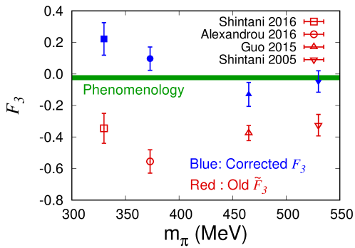
Figure 3: Recent lattice results of $F_{3}$ induced by the QCD $\Theta$-term calculated with $M_{\pi}<550$ MeV. Red points are the original results, which give $\tilde{F}_{3}$, and the blue points are the corrected results. Original results are obtained from Refs. Shintani:2015vsx (labeled Shintani 2016), Alexandrou:2015spa (Alexandrou 2016), Guo:2015tla (Guo 2015), and Shintani:2005xg (Shintani 2005), and the corrected results are obtained from Refs. Abramczyk:2017oxr ; Shintani:priv_com . As noted in Ref. Abramczyk:2017oxr , some assumptions are made to calculate the corrected $F_{3}$ numbers as some of the original papers do not contain full information needed for the parity induced rotation Eq. (14), so the $F_{3}$ results presented in this plot may not be precise.

4 quark EDM

The electromagnetic current, $V_{\mu}\equiv\delta\cal{L}/\delta A_{\mu}$, gets an additional contribution when the quark EDM operator is added to $\cal{L}_{\rm SM}$. Thus, while the standard conserved vector current interacts with a quark with charge $q_{f}$, this additional contribution, which is is just the flavor diagonal tensor operator for each quark flavor, couples with strength $d_{f}^{\gamma}g_{T}^{f}$, where $d_{f}^{\gamma}$ are the BSM model dependent CP violating couplings and $g_{T}^{u}$, $g_{T}^{s}$, $g_{T}^{s}$, $\ldots$ are the tensor charges, i.e., matrix elements of the quark bilinear tensor operator within the nucleon states. Furthermore, the effects analogous to the mixing discussed in Section 3 are suppressed by powers of the electromagnetic coupling $\alpha_{\rm EM}\sim 1/137$. Thus, the leading contribution of the EDM of the quarks to the nEDM is given by the flavor diagonal tensor charges:

$$\big{\langle}N|\bar{q}\sigma_{\mu\nu}q|N\big{\rangle}=g_{T}^{q}\bar{u}_{N}\sigma_{\mu\nu}u_{N}\,,$$

$$d_{N}=d_{u}g^{u}_{T}+d_{d}g^{d}_{T}+d_{s}g^{s}_{T}\,.$$ (15)

In many models, such as the supersymmetric models, the quark EDMs are proportional to the corresponding quark masses ($d_{q}\propto m_{q}$), because in these theories all connections between left and right-handed quarks are mediated by a common set of Yukawa interactions. Since the strange quark is much heavier than the u and the d quarks, the strange quark contribution gets enhanced, by $m_{s}/m_{d}\approx 20$. On the other hand $g_{T}^{s}\ll g_{T}^{l}$. Since the contribution is the product of the two, it is, therefore, important to determine the strange quark, and perhaps even the charm quark, tensor charge precisely.

There are two classes of diagrams in the calculation of flavor diagonal tensor charges: quark-line connected and the quark-line disconnected diagrams as illustrated in Figure 4. In case of the strange (charm) quark tensor charge, only the disconnected diagram with strange (charm) quark loop contributes. This is the basis of the expectation that $g_{T}^{s}\ll g_{T}^{l}$.

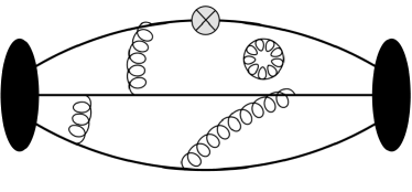
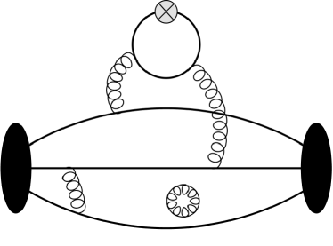
Figure 4: Quark-line connected (left) and disconnected (right) diagrams contribute to the quark EDM. Black ellipses are the neutrons, and the cross is the quark bilinear operator with tensor structure.

In Refs. Bhattacharya:2015esa ; Bhattacharya:2015wna , the tensor charges were calculated using clover fermions on the HISQ lattices, and extrapolated to continuum and physical pion mass limit, as illustrated in Figure 5 (left). The disconnected diagrams were estimated using a stochastic method, and it turned out that the disconnected diagram contribution to the tensor charges is very small. Their results are

$$g_{T}^{u}=-0.23(3),\quad g_{T}^{d}=0.79(7),\quad g_{T}^{s}=0.008(9)\,.$$ (16)

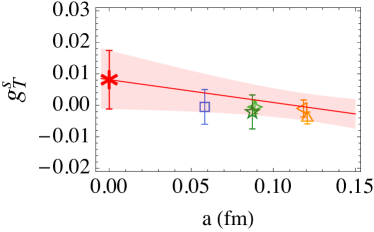
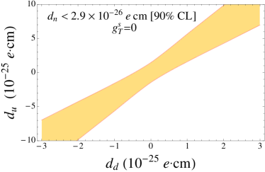
Figure 5: (Left) Extrapolation of $g_{T}^{s}$ to the continuum limit. The fit is performed simultaneously in $a$ and $M_{\pi}$ but only the projection to the $a$-plane with data extrapolated to the physical $M_{\pi}$, is presented. (Right) Bounds on $d_{u}$ and $d_{d}$ are obtained using the formula given in Eq. (15), the tensor charges given in Eq. (16) and the experimental bounds $|d_{N}|<2.9\times 10^{-26}e{\cdot}\textrm{cm}$. Since the strange quark tensor charge is consistent with zero within statistics, it imposes no constraint on $d_{s}$. Both figures are taken from Ref. Bhattacharya:2015esa .

There are BSM models in which the quark EDMs are the dominant sources of CP violation at low energy. In these scenarios, constraints can be placed on the couplings of the EDM of each quark flavor using the experimental bound on the neutron EDM and the lattice results for the tensor charges. Neglecting all other sources of CP violation, figure 5 (right) shows the allowed region of $d_{u}$ and $d_{d}$ using the lattice results, Eq. (16), described in Ref. Bhattacharya:2015esa ; Bhattacharya:2015wna . Of all the CP violating operators listed in Eq. (1), the calculation of the quark EDM, including renormalization, is theoretically well-established and the results in Eq. (16) for $g_{T}^{u}$ and $g_{T}^{d}$ indicate that these are already available at the $15\%$ level. Further improvement in precision will occur as higher precision data are generated in future calculations.

5 Quark Chromo-EDM

The last dimension-5 term is the quark chromo-electric dipole moment (cEDM) operator. The modification to the action in presence of the CP violating cEDM term is:

$$S=S_{QCD}-\frac{i}{2}\int d^{4}x\ \tilde{d}_{q}\bar{q}(\sigma\cdot G)\gamma_{5}q\,,$$ (17)

where $\tilde{d}_{q}$ are again BSM couplings evolved to the hadronic scale for each quark flavor. The lattice calculation consists of evaluating the matrix element of the insertion of the product of the electromagnetic current $V_{\mu}$ and the $\bar{q}(\sigma\cdot G)\gamma_{5}q$ operator within the neutron states. Then, the contribution of cEDM operators to the nEDM, ignoring the complicated operator mixing problem under renormalization discussed in Section 5.4 below, is obtained from $\sum_{q}\tilde{d}_{q}\langle N|V_{\mu}\bar{q}(\sigma\cdot G)\gamma_{5}q|N\rangle$.

Lattice QCD studies of the cEDM operator have started only recently, and three methods are being explored: an expansion in $\tilde{d}_{q}$ Abramczyk:2017oxr , external electric field method Abramczyk:2017oxr , and the Schwinger source method Bhattacharya:2016oqm ; Bhattacharya:2016rrc .

5.1 Expansion in $\tilde{d}_{q}$

The expansion in $\tilde{d}_{q}$ method proceeds analogously to the expansion in ${{\theta}}$ in the QCD $\Theta$-term calculation. For small BSM cEDM couplings, $\tilde{d}_{q}$, the neutron matrix element of the electromagnetic current can be written in terms of the expectation values evaluated on the standard CP even lattices,

$$\big{\langle}NV_{\mu}\bar{N}\big{\rangle}_{CPV} =\big{\langle}NV_{\mu}\bar{N}\big{\rangle}+\tilde{d}_{q}\Big{\langle}NV_{\mu}\bar{N}\cdot\sum_{x}O_{\mathrm{c}EDM}(x)\Big{\rangle}+\mathcal{O}(\tilde{d}_{q}^{2})\,,$$ (18)

$$O_{\mathrm{c}EDM} =\frac{i}{2}\bar{q}(\sigma\cdot G)\gamma_{5}q\,.$$ (19)

Their contribution to the neutron EDM is extracted from the CP violating form factor, $F_{3}$ as defined in Eq. (5). The calculation is challenging because it requires calculating the expectation value of four-point functions because one has to insert both the vector current and the cEDM operator between the neutron source and sink, with the cEDM operator defined as a sum over all space-time points.

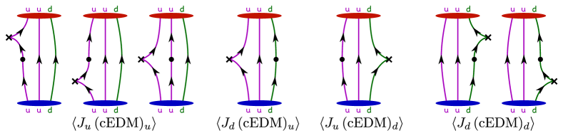
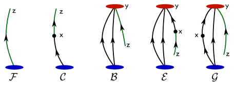
Figure 6: (Top) Connected diagrams needed for the calculation of the cEDM operator. Crosses are the cEDM operator insertion, and dots are the vector current insertion. (Bottom) Propagators needed for the quark-line connected four-point correlators. In this figure, the electromagnetic current is denoted as $J$. Figures are taken from Ref. Abramczyk:2017oxr .

Figure 6 (top) shows all the required quark-line connected diagrams. These four-point correlators are constructed using five types of propagators used as building blocks that are shown in the bottom panel of Figure 6 (bottom). $\mathcal{F}$ and $\mathcal{B}$ are the usual forward and backward propagators. $\mathcal{C}$ is the cEDM-sequential propagator. It is constructed by starting with the regular quark propagator and inserting the chromo-EDM operator at all lattice sinks points. This is then used as the source for calculating the chromo-EDM inserted propagator.

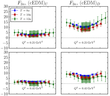
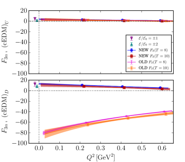
Figure 7: (Left) Plateau plots for $F_{3}$ induced by the cEDM operator calculated by expanding in $\tilde{d}_{q}$. Simulations were performed on $24^{3}\times 64$, $a=0.11$ fm and $M_{\pi}=340$ MeV DWF lattices. (Right) Results for cEDM contribution to $F_{3}$ extrapolated to $Q^{2}=0$ from the $\tilde{d}_{q}$-expansion results compared with the $F_{3}$ obtained by using the external electric field method. OLD and NEW $F_{3}$ label the results before and after fixing the parity mixing rotation given in (14). Same lattices used in (left) plot are used for this calculation. $\mathcal{E}_{0}=0.039\leavevmode\nobreak\ \mathrm{GeV}^{2}$. Note that these results are not renormalized. Figures are taken from Ref. Abramczyk:2017oxr .

Results from Ref. Abramczyk:2017oxr for the signal in $F_{3}$ and the source-sink separation dependence of the signal are shown in Figure 7 (left). $F_{3}$ has larger value when the cEDM is inserted in the d-quarks of the neutron. In Figure 7 (right), the results are extrapolated to zero-momentum to obtain the contribution $F_{3}(0)$ as needed for the neutron EDM.

5.2 External Electric Field Method

The chromo-EDM contribution to the neutron EDM also can be calculated using the external electric field. Similarly to the QCD $\Theta$-term, the neutron EDM is extracted from the energy difference of nucleon states under spin flip in presence of a uniform external electric field $i\mathcal{E}$:

$$E^{\mathrm{cEDM}}_{\vec{S}}-E^{\mathrm{cEDM}}_{-\vec{S}}\approx 2d_{N}\vec{S}\cdot i\vec{\mathcal{E}}\,,$$ (20)

where the neutron correlators in the presence of the cEDM term are obtained by reweighting,

$$\big{\langle}N\bar{N}\big{\rangle}_{\mathrm{cEDM}}(i\vec{\mathcal{E}},t)=\big{\langle}N(t)\bar{N}(0)O_{\mathrm{cEDM}}\big{\rangle}_{i\vec{\mathcal{E}}}\,.$$ (21)

This method needs only two- and three-point functions of the neutron, the latter with the insertion of the cEDM bilinear operator. In Ref. Abramczyk:2017oxr , $F_{3}$ is extracted using the external electric field method on the same ensemble of lattices used for the calculation using the $\tilde{d}_{q}$-expansion method, and the results are presented in Figure 7 (right). The signal is poorer in the external electric field method compared to those in expansion in $\tilde{d}_{q}$ method, but the results of the two methods are consistent. Note that the external electric field method is not affected by the parity mixing problem described in Section 3, while the $\tilde{d}_{q}$-expansion method is. Therefore, the consistency of the results from the two methods, after taking care of the parity mixing rotation given in (14), suggests that both methods are yielding a reliable signal.

5.3 Schwinger Source Method

Another method to calculate the contribution of the cEDM operator to the neutron EDM is the Schwinger source method Bhattacharya:2016oqm ; Bhattacharya:2016rrc . Noting that the cEDM operator is a quark bilinear, $i\bar{q}(\sigma\cdot G)\gamma_{5}q$, one can add it to the QCD fermion action:

$$D_{\mathrm{clov}}\longrightarrow D_{\mathrm{clov}}+i\varepsilon\sigma^{\mu\nu}\gamma_{5}G_{\mu\nu}\,,$$ (22)

where $D_{\mathrm{clov}}$ is the Dirac operator for the Wilson-clover action, and $\varepsilon$ is a small control parameter the dependence on which will be removed by taking a derivative with respect to it at the end of the calculation. Because cEDM is a quark bilinear, the integration over the fermion degrees of freedom in the path integral can still be carried out as before. In the case of the clover fermions, the addition of the cEDM operator is equivalent to shifting the coefficient of the dimension-5 clover term by $i\varepsilon\gamma_{5}$:

$$c_{\mathrm{sw}}\sigma^{\mu\nu}G_{\mu\nu}\longrightarrow\sigma^{\mu\nu}(c_{\mathrm{sw}}+i\varepsilon\gamma_{5})G_{\mu\nu}\,.$$ (23)

In this approach, the insertion of the cEDM term is carried out by calculating valence quark propagators including this modified clover term, and using this propagator in all diagrams requiring a cEDM insertion. Having taken care of the cEDM term, the calculation of the original 4-point functions reduces to three-point functions, with an insertion of the vector current within the neutron state, made up of propagators with and without cEDM insertion.

To perform this calculation on ensembles generated with just the standard QCD action, however, requires taking into account the change in the Boltzmann factor under the addition of the cEDM term to the action as shown in Eq. (22). This, a priori, non-unitary formulation between sea and valence quarks can be accounted for at leading order in $\varepsilon$ by reweighting each configuration by ratio of the fermion determinant with and without the cEDM term:

$$\frac{\det\Big{(}D_{\mathrm{clov}}+i\varepsilon\sigma^{\mu\nu}\gamma_{5}G_{\mu\nu}\Big{)}}{\det\Big{(}D_{\mathrm{clov}}\Big{)}}\approx\exp\Big{[}i\varepsilon\mathrm{Tr}\big{(}\sigma^{\mu\nu}\gamma_{5}G_{\mu\nu}D_{\mathrm{clov}}^{-1}\big{)}\Big{]}\,.$$ (24)

Diagrammatically, all the terms that need to be calculated in this Schwinger source method are shown in Figure 8. There are three classes of diagrams at leading order in $\varepsilon$: the reweighting factor for each configuration, and the quark-line connected and disconnected diagrams on that configuration.

Figure 8: Quark line diagrams needed for the Swinger source method. The reweighting factor (left), the quark-line disconnected (middle four), and the quark-line connected (right four) diagrams. Red crossed box is the cEDM operator insertion, $P$ is the regular quark propagator without the cEDM operator insertion, and $P_{\varepsilon}$ is the quark propagator with the cEDM operator insertion. An identical calculation has to be done with the cEDM operator replaced by the $\gamma_{5}$ operator in order to define a finite renormalized quantity.

Current calculations are at the stage of demonstrating a signal in the full evaluation of Figure 8 with both the cEDM and the $\gamma_{5}$ operator with which it mixes under renormalization as discussed in Section 5.4. First, in Figure 9, we show the success at extraction of the phase $\alpha$ that is induced in the ground state nucleon spinor by the CP violating cEDM and $\gamma_{5}$ operators. In the right panel of Figure 9, we also show that this $\alpha$ is linear in $\varepsilon$, which allows us to tune the value of $\varepsilon$. We want to use a large $\varepsilon$ to increase the signal but remain in the linear response regime.

First examples of the quality of the signal in the contribution of the connected diagrams to the form factor $F_{3}$ induced by the cEDM and $\gamma_{5}$ operators are shown in Figures 10 for two different source and sink separations. At present, the signal is consistent with zero for both operators.

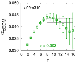
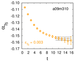
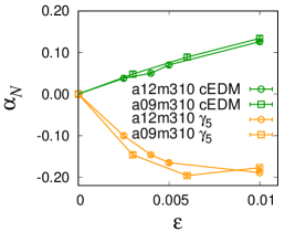
Figure 9: The left panel shows the extraction of the CP violating phase $\alpha$ induced by the cEDM operator from the long-time behavior of the 2-point correlator. The middle panel shows the extraction of the phase for the $\gamma_{5}$ operator insertion. The right panel shows that both kinds of phases are linear in $\varepsilon$ when $\varepsilon$ is small. These data are from the Clover-on-HISQ analysis on the $M_{\pi}\approx 310$ MeV ensembles with lattice spacing $a=0.12$ (a12m310) and $0.09$ (a09m310) fm.

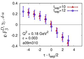
Figure 10: (Left) Signal of $F_{3}$ form-factor for two different separation of source and sink on a09m310 lattices. cEDM is inserted on d-quarks. Only the connected diagrams are considered. (Right) Same plot as the (middle), but $\gamma_{5}$ is inserted instead of the cEDM operator. Results shown are for the bare operators.

5.4 Renormalization of cEDM Operator

The renormalization of the cEDM operator is studied both in one-loop perturbation theory with Twisted-mass fermions Constantinou:2015ela , and in nonperturbative RI-SMOM scheme Bhattacharya:2015rsa . The most challenging outcome is the divergent mixing with lower-dimensional operators: in particular the $1/a^{2}$ mixing with the pseudoscalar quark bilinear operator:

$$O_{\mathrm{cEDM}}=a^{2}\bar{q}\sigma^{\mu\nu}\gamma_{5}G_{\mu\nu}q,\qquad O_{P}=\bar{q}\gamma_{5}q\,.$$ (25)

Because the mixing is $1/a^{2}$ divergent, it needs to be calculated precisely so that a finite operator can be constructed, ensemble by ensemble, by subtracting the two terms. In Ref. Constantinou:2015ela , the authors presented the results of the $1/a^{2}$ mixing coefficients for the Twisted-mass fermions calculated non-perturbatively and using the one-loop perturbation theory. In Ref. Bhattacharya:2015rsa , authors defined a momentum subtraction scheme, RI-$\tilde{\text{S}}$MOM, for the non-perturbative renormalization of the cEDM operator on the lattice, and provided one-loop matching coefficients to the $\overline{\text{MS}}$ scheme in continuum limit.

6 Summary

In this talk, we reviewed the recent lattice QCD calculations of the contribution of dimension four and five CP violating operators to the EDM of the neutron.

We reviewed the three approaches, external electric field method, expansion in ${{\theta}}$, and simulation with imaginary ${{\theta}}$, used for the calculation of the QCD $\Theta$-term in Section 2. We also summarized the observation made in Ref. Abramczyk:2017oxr concerning the subtlety of properly defining the neutron spinor in the presence of parity violating interactions and its consequences vis-a-vis mixing between the form factors $F_{2}$ and $F_{3}$ in Section 3. All calculations based on extracting $F_{3}$, previous to Ref. Abramczyk:2017oxr , had missed this mixing. After correction, current lattice QCD results for the QCD $\Theta$-term, are reduced by about a factor of ten and do not show a statistically significant non-zero signal.

The quark EDM contribution to the neutron EDM can be written in terms of the neutron tensor charges $g_{q}^{T}$. Currently, the $g_{u,d}^{T}$ are determined to within 15% uncertainty including the quark-line disconnected diagrams, and $g_{s}^{T}$ is known to be very small. The results are summarized in Section 4.

Lattice QCD calculation for the quark chromo-EDM operator have just started. Three methods for the calculation of the contribution of cEDM and the construction of a finite renormalized operator are described in Section 5. The methodology for calculation of the 3-point (or 4-point) correlation functions is under control but a non-zero signal in all the diagrams has yet to be demonstrated. Once a signal is achieved, we will still be a long way away from a full calculation due to the divergent mixing between the cEDM and $\gamma_{5}$ operators.

A few brief words on other lattice QCD calculations related to the neutron EDM that have not been covered in this review. First, preliminary results for the Weinberg three-gluon operator, one of the dimension-six operators, were presented at the Lattice 2017 conference Dragos:2017talk . Calculations of the Weinberg operator are at the stage of demonstrating a signal and have not even begun to address the issue of renormalization that is potentially even more complicated than that for the cEDM operator. Calculations exploring the four-fermion dimension six operators are yet to begin. Second, there are efforts to study the neutron EDM using lattice spectroscopy, and other matrix elements combined with chiral perturbation theory deVries:2016jox , in addition to the direct calculation of the matrix elements with the CP violating operators.

To summarize, the theoretical calculations of matrix elements needed to extend the importance and reach of nEDM experiments to constrain BSM physics have begun in earnest but are very challenging and will require many new innovations in both theory and computations.

References

- (1) J.M. Pendlebury et al., Phys. Rev. D92, 092003 (2015), 1509.04411
- (2) Search for the neutron electric dipole moment at PSI, https://www.psi.ch/nedm/
- (3) R. Picker, JPS Conf. Proc. 13, 010005 (2017), 1612.00875
- (4) A next generation measurement of the electric dipole moment of the neutron at the FRM-II, http://nedm.ph.tum.de/
- (5) Search for a neutron electric dipole moment at the SNS, http://fsnutown.phy.ornl.gov/fsnufiles/positionpapers/FSN_position_nEDM_2014_5.pdf
- (6) A cryogenic experiment to search for the EDM of the neutron, http://hepwww.rl.ac.uk/EDM/index_files/CryoEDM.htm
- (7) S. Dar (2000), hep-ph/0008248
- (8) M. Pospelov, A. Ritz, Annals Phys. 318, 119 (2005), hep-ph/0504231
- (9) M.J. Ramsey-Musolf, S. Su, Phys. Rept. 456, 1 (2008), hep-ph/0612057
- (10) J. Engel, M.J. Ramsey-Musolf, U. van Kolck, Prog.Part.Nucl.Phys. 71, 21 (2013), 1303.2371
- (11) A. Sakharov, Pisma Zh.Eksp.Teor.Fiz. 5, 32 (1967)
- (12) W. Bernreuther, Lect. Notes Phys. 591, 237 (2002), [,237(2002)], hep-ph/0205279
- (13) M. Pospelov, A. Ritz, Nucl. Phys. B573, 177 (2000), hep-ph/9908508
- (14) R.J. Crewther, P. Di Vecchia, G. Veneziano, E. Witten, Phys. Lett. 88B, 123 (1979), [Erratum: Phys. Lett.91B,487(1980)]
- (15) A. Abada, J. Galand, A. Le Yaouanc, L. Oliver, O. Pene, J.C. Raynal, Phys. Lett. B256, 508 (1991)
- (16) E. Mereghetti, J. de Vries, W.H. Hockings, C.M. Maekawa, U. van Kolck, Phys. Lett. B696, 97 (2011), 1010.4078
- (17) R.D. Peccei, H.R. Quinn, Phys. Rev. Lett. 38, 1440 (1977)
- (18) R.D. Peccei, H.R. Quinn, Phys. Rev. D16, 1791 (1977)
- (19) S. Aoki, A. Gocksch, Phys. Rev. Lett. 63, 1125 (1989), [Erratum: Phys. Rev. Lett.65,1172(1990)]
- (20) S. Aoki, A. Gocksch, A.V. Manohar, S.R. Sharpe, Phys. Rev. Lett. 65, 1092 (1990)
- (21) E. Shintani, S. Aoki, N. Ishizuka, K. Kanaya, Y. Kikukawa, Y. Kuramashi, M. Okawa, A. Ukawa, T. Yoshie, Phys. Rev. D75, 034507 (2007), hep-lat/0611032
- (22) E. Shintani, S. Aoki, Y. Kuramashi, Phys. Rev. D78, 014503 (2008), 0803.0797
- (23) E. Shintani, S. Aoki, N. Ishizuka, K. Kanaya, Y. Kikukawa, Y. Kuramashi, M. Okawa, Y. Tanigchi, A. Ukawa, T. Yoshie, Phys. Rev. D72, 014504 (2005), hep-lat/0505022
- (24) F. Berruto, T. Blum, K. Orginos, A. Soni, Phys. Rev. D73, 054509 (2006), hep-lat/0512004
- (25) A. Shindler, T. Luu, J. de Vries, Phys. Rev. D92, 094518 (2015), 1507.02343
- (26) C. Alexandrou, A. Athenodorou, M. Constantinou, K. Hadjiyiannakou, K. Jansen, G. Koutsou, K. Ottnad, M. Petschlies, Phys. Rev. D93, 074503 (2016), 1510.05823
- (27) E. Shintani, T. Blum, T. Izubuchi, A. Soni, Phys. Rev. D93, 094503 (2016), 1512.00566
- (28) T. Izubuchi, S. Aoki, K. Hashimoto, Y. Nakamura, T. Sekido, G. Schierholz, PoS LAT2007, 106 (2007), 0802.1470
- (29) S. Aoki, R. Horsley, T. Izubuchi, Y. Nakamura, D. Pleiter, P.E.L. Rakow, G. Schierholz, J. Zanotti (2008), 0808.1428
- (30) F.K. Guo, R. Horsley, U.G. Meissner, Y. Nakamura, H. Perlt, P.E.L. Rakow, G. Schierholz, A. Schiller, J.M. Zanotti, Phys. Rev. Lett. 115, 062001 (2015), 1502.02295
- (31) M. Abramczyk, S. Aoki, T. Blum, T. Izubuchi, H. Ohki, S. Syritsyn, Phys. Rev. D96, 014501 (2017), 1701.07792
- (32) K.F. Liu, J. Liang, Y.B. Yang (2017), 1705.06358
- (33) Private communication with Eigo Shintani.
- (34) T. Bhattacharya, V. Cirigliano, R. Gupta, H.W. Lin, B. Yoon, Phys. Rev. Lett. 115, 212002 (2015), 1506.04196
- (35) T. Bhattacharya, V. Cirigliano, S. Cohen, R. Gupta, A. Joseph, H.W. Lin, B. Yoon (PNDME), Phys. Rev. D92, 094511 (2015), 1506.06411
- (36) T. Bhattacharya, V. Cirigliano, R. Gupta, E. Mereghetti, B. Yoon, PoS LATTICE2015, 238 (2016), 1601.02264
- (37) T. Bhattacharya, V. Cirigliano, R. Gupta, B. Yoon, PoS LATTICE2016, 225 (2016), 1612.08438
- (38) M. Constantinou, M. Costa, R. Frezzotti, V. Lubicz, G. Martinelli, D. Meloni, H. Panagopoulos, S. Simula, Phys. Rev. D92, 034505 (2015), 1506.00361
- (39) T. Bhattacharya, V. Cirigliano, R. Gupta, E. Mereghetti, B. Yoon, Phys. Rev. D92, 114026 (2015), 1502.07325
- (40) J. Dragos, A. Shindler, T. Luu, J. de Vries (2017), Lattice 2017 conference, https://makondo.ugr.es/event/0/session/95/contribution/249
- (41) J. de Vries, E. Mereghetti, C.Y. Seng, A. Walker-Loud, Phys. Lett. B766, 254 (2017), 1612.01567