Analysis of a model for hepatitis C virus transmission that
includes the effects of vaccination with waning immunity

Abstract

This paper considers a mathematical model based on the transmission dynamics of hepatitis C virus (HCV) infection. In addition to the usual compartments for susceptible, exposed, and infected individuals, this model includes compartments for individuals who are under treatment and those who have had vaccination against HCV infection. It is assumed that the immunity provided by the vaccine fades with time. The basic reproduction number, $R_{0}$, and the equilibrium solutions of the model are determined. The model exhibits the phenomenon of backward bifurcation where a stable disease-free equilibrium co-exists with a stable endemic equilibrium whenever $R_{0}$ is less than unity. It is shown that the use of only a perfect vaccine can eliminate backward bifurcation completely. Furthermore, a unique endemic equilibrium of the model is proved to be globally asymptotically stable under certain restrictions on the parameter values. Numerical simulation results are given to support the theoretical predictions. [epidemiological model; equilibrium solutions; backward bifurcation; global asymptotic stability; Lyapunov function.]

1 Introduction

The liver of a hepatitis patient is one of the most frequently damaged organs in the body, and it is indeed fortunate that it has a very large functional reserve. In the experimental animal, it has been shown that only 10% of the hepatic parenchyma (the functional part of the liver) is required to maintain normal liver function (Cotran et al. 1994). The liver can be infected due to a variety of infectious agents such as parasites, viruses, and bacteria, and diseases of the liver have a variety of causes such as obstructive, vascular, metabolic and toxic involvements.

Hepatitis C is the inflammation of the liver caused by hepatitis C virus (HCV), and spreads through contact with contaminated blood. Hepatitis C may be an acute infection, which spans over a period of weeks to a few months, or chronic infection, in which the virus persists for a longer time (Di Bisceglie 2000; Das et al. 2005). Acute hepatitis is characterized by moderate liver injury and if symptoms appear, they include fatigue, loss of appetite, abdominal pain, fever and jaundice. However, most of the times, acute hepatitis is asymptomatic. A large percentage of patients with HCV infection recover completely, but some develop long term chronic hepatitis or massive necrosis of the liver. Chronic HCV infection may damage the liver permanently, cause cirrhosis, hepatic failure, and sometimes liver cancer.

Today, HCV infects an estimated 170 million people worldwide (Qesmi et al. 2010). Around 150 million people are chronically infected with HCV. HCV infection is a major cause of death of more than 350,000 people every year. Countries with the highest prevalence of chronic liver infection are Egypt (15%), Pakistan (4.8%) and China (3.2%) (Lozano 1990). Although, treatment for this infection does exist, the current drug therapies are ineffective in completely eliminating the virus and patients suffering from chronic illness may require a liver transplant (Qesmi et al. 2010). Unfortunately, there is no effective vaccine yet developed that may help prevent the spread of the disease. At present, various attempts are being made to create such a vaccine (Chen and Li 2006). Thus, it is crucial to assess the potential impact of HCV vaccine on the population.

Some mathematical models on HCV infection have been formulated recently, but much work has not been done, since it is a relatively new disease (discovered in 1989) and data is not available on account of the high variability of the HCV. In contrast, more research has been carried out on hepatitis B virus (HBV) infection. Several epidemiological models have focused on the effects of preventive measures as well as control of HBV infection (Zhang and Zhou 2012). This has helped in creating cost effective disease prevention techniques. The modes of transmission of both HCV and HBV are same, i.e. through blood, thus mathematical models on both infections are somewhat inter related. Some mathematical models were formed on HCV infection that considered infected cells, uninfected cells and viral cells in the human host. The basic aim of these models was to study the effects of liver transplant in patients with HCV infection. But in major cases, HCV infection is not completely eliminated even after the transplant. Thus, these models were extended to include more infected compartments (Dahari et al. 2005). Martcheva and Castillo-Chavez (2003) introduced an epidemiologic model of HCV infection with chronic infectious stage in a varying population. Their model does not include a recovered or immune class and it falls within the susceptible-infected- susceptible (SIS) category of models. A susceptible-infected-recovered (SIR) model was used by Jager et al. (2004) to study the transmission of HCV among injecting drug users, while susceptible-infected-removed-susceptible (SIRS) type models that allow waning immunity are presented in Zeiler et al. (2010). Also, a deterministic model for HCV transmission is used by Elbasha (2013), with the objective of assessing the impact of therapy on public health.

Our aim is to meticulously analyze the model and examine various parameters to explore their effect on the transmission of HCV and its control. The model focuses on studying the effects of imperfect vaccines on the control of hepatitis C. The model shows that an imperfect vaccine reduces the number of individuals who are exposed to HCV, while a perfect vaccine completely removes them. We have subdivided the total population into six mutually-exclusive compartments of susceptible, exposed, acutely infected, chronically infected, treated and vaccinated individuals. Ordinary differential equations are used to model the HCV infection. This model can help provide insights into the spread of HCV infection and the assessment of the effectiveness of immunization techniques.

This paper is organized as follows: The mathematical model is developed and analyzed in Section 2. The stability of the disease free equilibrium, and the endemic equilibrium is discussed, along with the effects of vaccination on backward bifurcation phenomenon. Numerical simulations are also provided in the same section. Section 3 summarizes the final results of the paper.

2 Model Formulation

The total population at time $t$, denoted by $N(t)$, is divided into sub-populations of susceptible individuals, $S(t)$, exposed individuals with hepatitis C symptoms, $E(t)$, individuals with acute infection, $I(t)$, individuals undergoing treatment, $T(t)$, individuals with chronic infection, $C_{h}(t)$, and vaccinated individuals, $V(t)$, so that

$$N(t)=S(t)+E(t)+I(t)+T(t)+C_{h}(t)+V(t).$$

It is assumed that the mode of transmission of HCV infection is horizontal. We further assume that mixing of individual hosts is homogeneous (every person in the population $N(t)$ has an equal chance of getting HCV infection). The following system of ordinary differential equations describes the dynamics of the HCV infection

$$\begin{array}[]{rcl}\displaystyle\frac{dS}{dt}&=&(1-b)\Lambda+\rho T+\alpha V-(\beta_{1}I+\beta_{2}C_{h}+\beta_{3}T)S+\sigma C_{h}-\mu S,\cr\cr\displaystyle\frac{dE}{dt}&=&(\beta_{1}I+\beta_{2}C_{h}+\beta_{3}T)S+(1-\psi)(\beta_{1}I+\beta_{2}C_{h}+\beta_{3}T)V-(\epsilon+\mu)E,\cr\cr\displaystyle\frac{dI}{dt}&=&\epsilon E-(\kappa+\mu)I,\cr\cr\displaystyle\frac{dT}{dt}&=&\pi_{1}\kappa I+\pi_{2}C_{h}-(\rho+\mu)T,\cr\cr\displaystyle\frac{dC_{h}}{dt}&=&(1-\pi_{1})\kappa I-(\pi_{2}+\sigma+\mu)C_{h},\cr\cr\displaystyle\frac{dV}{dt}&=&b\Lambda-(\alpha+\mu)V-(1-\psi)(\beta_{1}I+\beta_{2}C_{h}+\beta_{3}T)V.\end{array}$$ (2.1)

The recruitment rate of susceptible humans is $\Lambda$. A proportion, $b$, of these susceptible individuals is vaccinated. The death rate of individuals is denoted by $\mu$. The rate of progression from acute infected class to both treated and chronic infected class is given by $\kappa$. The acutely infected proportion of individuals who enter the treated class is $\pi_{1}$. The remaining infected proportion, $(1-\pi_{1})$, progresses to the chronic infectious stage. The rate of progression for treatment from chronic hepatitis is given by $\pi_{2}$. The term $\epsilon$ is the rate of progression from exposed class to acute infected class. The recovery rates due to treatment and naturally from the chronic group are $\rho$ and $\sigma$, respectively.

The transmission coefficients of HCV infection by individuals with acute hepatitis C, $I(t)$, chronic hepatitis C, $C_{h}(t)$ and individuals undergoing treatment but not yet cured, $T(t)$ are $\beta_{1},\beta_{2},$ and $\beta_{3}$, respectively. Following effective contact with $I(t)$, $C_{(}t)$, and $T(t)$, susceptible individuals can acquire HCV at a rate $(\beta_{1}I+\beta_{2}C_{h}+\beta_{3}T)$. $\psi$ ($0<\psi\leq 1$) represents the vaccine efficacy, with $\psi=1$ representing a perfect vaccine, and $\psi\in(0,1)$ corresponding to an imperfect vaccine which wanes with time. The term $(1-\psi)$ corresponds to the decrease in disease transmission in vaccinated individuals, in contrast to susceptible individuals who are not vaccinated. Hence, vaccinated individuals acquire HCV at a reduced rate $(1-\psi)(\beta_{1}I+\beta_{2}C_{h}+\beta_{3}T)$. The rate at which the vaccine wanes is denoted by $\alpha$. The parameter description is described in Table 1.

Table 1: Description of parameters

Parameter	Description
$\Lambda$	recruitment rate of individuals
$\mu$	death rate of individuals
$\alpha$	waning rate of the vaccine
$\psi$	vaccine efficacy
$\beta_{i}$	transmission rate (i=1, 2, 3)
$b$	proportion of vaccinated individuals
$\kappa$	rate of progression from the acute state
	to treated and chronic state
$\epsilon$	rate of transfer from exposed class
	to acute infected class
$\pi_{1}$	proportion of individuals who enter
	the treated class from acutely infected class
$\pi_{2}$	rate of progression for treatment
	from chronic hepatitis
$\rho$	rate of recovery due to treatment
$\sigma$	rate of recovery from the chronic class

In the proposed model (2.1), the total population is $S+E+I+T+C_{h}+V=\frac{\Lambda}{\mu}\$ for all $t\geq 0$, provided that $S(0)+E(0)+I(0)+T(0)+C_{h}(0)+V(0)=\frac{\Lambda}{\mu}.$ Thus, the biologically feasible region for system (2.1) given by

$$\Delta=\{(S,E,I,T,C_{h},V)\in R^{6}:S+E+I+T+C_{h}+V=\displaystyle\frac{\Lambda}{\mu}\},$$

is positively invariant with respect to the system (2.1).

2.1 Local stability of the disease-free equilibrium (DFE)

For the mathematical model in equation (2.1), the DFE, $P_{0}$ is given by

$$(S_{0},E_{0},I_{0},T_{0},C_{h0},V_{0})=\Big{(}\displaystyle\frac{(1-b)\Lambda}{\mu}+\frac{\alpha b\Lambda}{\mu(\alpha+\mu)},0,0,0,0,\displaystyle\frac{b\Lambda}{\alpha+\mu}\Big{)}.$$

The local stability of $P_{0}$ is determined by the next generation operator method (Driessche and Watmough 2002) on system (2.1). For this purpose, the basic reproduction number (the average number of secondary infections produced by an infected individual in a completely susceptible population), denoted by $R_{0}$, is obtained. Using the same notation as in Driessche and Watmough (2002), $R_{0}$ is given by

$$R_{0}=\frac{\epsilon}{K_{1}K_{2}}(\displaystyle\frac{(1-b)\Lambda}{\mu}+\frac{\alpha b\Lambda}{\mu K_{5}}+(1-\psi)\displaystyle\frac{b\Lambda}{K_{5}})\Bigr{[}\beta_{1}+\beta_{2}\frac{\kappa(1-\pi_{1})}{K_{4}}+\beta_{3}\frac{\left(\pi_{1}\kappa K_{4}+\pi_{2}\kappa(1-\pi_{1})\right)}{K_{3}K_{4}}\Bigr{]},$$

where

$$K_{1}=\epsilon+\mu,~{}K_{2}=\kappa+\mu,~{}K_{3}=\rho+\mu,~{}K_{4}=\pi_{2}+\sigma+\mu,K_{5}=\alpha+\mu.$$

Using Theorem 2 in Driessche and Watmough (2002), the following result is established.

Theorem 2.1.

The DFE of the model (2.1), is locally asymptotically stable if $R_{0}<1$, and unstable if $R_{0}>1$.

2.2 Endemic equilibria and backward bifurcation

To calculate the endemic equilibrium, we consider the following reduced system of differential equations

$$\begin{array}[]{rcl}\displaystyle\frac{dE}{dt}&=&(\beta_{1}I+\beta_{2}C_{h}+\beta_{3}T)(\displaystyle\frac{\Lambda}{\mu}-E-I-T-C_{h}-\psi V)-K_{1}E,\cr\cr\displaystyle\frac{dI}{dt}&=&\epsilon E-K_{2}I,\cr\cr\displaystyle\frac{dT}{dt}&=&\pi_{1}\kappa I+\pi_{2}C_{h}-K_{3}T,\cr\cr\displaystyle\frac{dC_{h}}{dt}&=&(1-\pi_{1})\kappa I-K_{4}C_{h},\cr\cr\displaystyle\frac{dV}{dt}&=&b\Lambda-K_{5}V-(1-\psi)(\beta_{1}I+\beta_{2}C_{h}+\beta_{3}T)V.\end{array}$$ (2.2)

We will consider the dynamics of the flow generated by (2.2) in the invariant region

$$\Omega=\{E+I+T+C_{h}+V\leq\displaystyle\frac{\Lambda}{\mu}\}.$$

The endemic equilibrium for system (2.2) is $P^{*}(E^{\ast},I^{\ast},T^{\ast},C_{h}^{\ast},V^{\ast})$, where

$$\begin{array}[]{rcl}E^{\ast}&=&\displaystyle\frac{K_{2}I^{\ast}}{\epsilon},\cr\cr T^{\ast}&=&\displaystyle\frac{(\pi_{1}\kappa K_{4}+\pi_{2}(1-\pi_{1})\kappa)I^{\ast}}{K_{4}K_{3}},\cr\cr C_{h}^{\ast}&=&\displaystyle\frac{(1-\pi_{1})\kappa I^{\ast}}{K_{4}},\cr\cr V^{\ast}&=&\displaystyle\frac{b\Lambda}{K_{5}+(1-\psi)[\beta_{1}+\beta_{2}\displaystyle\frac{\kappa(1-\pi_{1})}{K_{4}}+\beta_{3}\frac{\left(\pi_{1}\kappa K_{4}+\pi_{2}\kappa(1-\pi_{1})\right)}{K_{3}K_{4}}]I^{\ast}},\end{array}$$ (2.3)

and $I^{\ast}$ is the root of the following quadratic equation

$$a_{1}I^{\ast 2}+a_{2}I^{\ast}+a_{3}=0.$$ (2.4)

Here

$$\begin{array}[]{rcl}a_{1}&=&(1-\psi)B^{2}[\mu K_{2}K_{3}K_{4}+\epsilon\mu\ K_{3}K_{4}+\left(\pi_{1}\kappa K_{4}+\pi_{2}\kappa(1-\pi_{1})\right)\epsilon\mu\cr\cr&&+\epsilon\kappa\mu(1-\pi_{1})K_{3}],\cr\cr a_{2}&=&B[\mu K_{2}K_{3}K_{4}K_{5}+\epsilon\mu K_{3}K_{4}K_{5}+\epsilon\mu K_{5}(\pi_{1}\kappa K_{4}+\pi_{2}(1-\pi_{1})\kappa)\cr\cr&&+(1-\pi_{1})\epsilon\kappa\mu K_{3}K_{5}+(1-\psi)\mu K_{1}K_{2}K_{3}K_{4}-(1-\psi)\Lambda\epsilon BK_{3}K_{4}],\cr\cr a_{3}&=&\mu K_{1}K_{2}K_{4}K_{3}K_{5}(1-R_{0}),\end{array}$$ (2.5)

with

$$B=\bigg{[}\beta_{1}+\beta_{2}\frac{\kappa(1-\pi_{1})}{K_{4}}+\beta_{3}\frac{(\pi_{1}\kappa K_{4}+\pi_{2}\kappa(1-\pi_{1}))}{K_{3}K_{4}}\bigg{]}.$$

The endemic equilibria of the model (2.2) can then be obtained by solving for $I^{\ast}$ from (2.4), and substituting the positive values of $I^{\ast}$ into the expressions in (2.3). Hence, $S^{\ast}$ can be determined from $\frac{\Lambda}{\mu}-E^{\ast}-I^{\ast}-T^{\ast}-C_{h}^{\ast}-V^{\ast}$. From (2.5), it can be seen that $a_{1}$ is always positive (for an imperfect vaccine), and $a_{3}$ is positive (negative) if $R_{0}$ is less than (greater than) unity. Thus, the following result is established

Theorem 2.2.

The model in (2.2) has:

(i) a unique endemic equilibrium if $a_{3}<0\Leftrightarrow R_{0}>1$;

(ii) a unique endemic equilibrium if $a_{2}<0$, and $a_{3}=0$ or $a_{2}^{2}-4a_{1}a_{3}=0$;

(iii) two endemic equilibria if $a_{3}>0,a_{2}<0$ and $a_{2}^{2}-4a_{1}a_{3}>0$;

(iv) no endemic equilibrium otherwise.

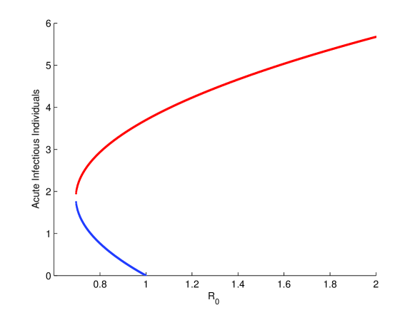
Figure 1: Backward Bifurcation diagram, with parameter values $\beta_{2}=0.09$, $\beta_{3}=0.19$, $\mu=0.00004$, $\alpha=0.1$, $\rho=0.152$, $\pi_{1}=0.001$, $\pi_{2}=0.02$, $\epsilon=0.022$, $\kappa=0.032$, $\Lambda=0.0052$, $\sigma=0.2$, $\psi=0.95$.

Hence, the model has a unique endemic equilibrium ($P^{*}$) whenever $R_{0}>1$, as evident from case (i) of the above theorem. Also, case (iii) indicates a possible chance of backward bifurcation (where a locally asymptotically stable DFE exists along with a locally asymptotically stable endemic equilibrium when $R_{0}<1$). Since, for $a_{3}>0$, $R_{0}<1$, the model will have a disease-free equilibrium and two endemic equilibria. To check for this, the discriminant $a_{2}^{2}-4a_{1}a_{3}$ is set to zero and is solved for the critical value of $R_{0}$. The critical value is denoted by $R_{c}$ and is given by

$$R_{c}=1-\frac{a_{2}^{2}}{4a_{1}\mu K_{1}K_{2}K_{5}K_{3}K_{4}}.$$

Backward bifurcation occurs for those values of $R_{0}$ which satisfy $R_{c}<R_{0}<1$. This is illustrated by simulating the model with these parameter values: $\beta_{1}=0.03$, $\beta_{3}=0.19$, $\mu=0.00004$, $\alpha=0.1$, $\rho=0.152$, $\pi_{1}=0.001$, $\pi_{2}=0.02$, $\epsilon=0.022$, $\kappa=0.032$, $\Lambda=0.0052$, $\sigma=0.2$, $\psi=0.95$. (These values are used merely for illustration purposes, and may not be realistic from epidemiological point of view.) The result is shown in Fig. 1. It can be seen that a locally asymptotically stable disease free equilibrium, a locally asymptotically stable endemic equilibrium, and, an unstable endemic equilibrium coexist when $R_{0}<1$.

2.2.1 Proof of backward bifurcation phenomenon

The phenomenon of backward bifurcation can be proved by using the center manifold theory on system (2.1). A theorem given by Castillo-Chavez and Song (2004) will be used here. To apply this method, the following change of variables is made on the model:

$$x_{1}=S,x_{2}=E,x_{3}=I,x_{4}=T,x_{5}=C_{h},x_{6}=V.$$

Let

$$X=(x_{1},x_{2},x_{3},x_{4},x_{5},x_{6})^{T}.$$

Thus, the system (2.1) can now be written as $\frac{dX}{dt}=(f_{1},f_{2},f_{3},f_{4},f_{5},f_{5},f_{6})^{T}$ and is given below

$$\begin{array}[]{rcl}\displaystyle\frac{dx_{1}}{dt}&=f_{1}=&(1-b)\Lambda+\rho x_{4}+\alpha x_{6}-(\beta_{1}x_{3}+\beta_{2}x_{5}+\beta_{3}x_{4})x_{1}+\sigma x_{5}-\mu x_{1},\cr\cr\displaystyle\frac{dx_{2}}{dt}&=f_{2}=&(\beta_{1}x_{3}+\beta_{2}x_{5}+\beta_{3}x_{4})x_{1}+(1-\psi)(\beta_{1}x_{3}+\beta_{2}x_{5}+\beta_{3}x_{4})x_{6}-K_{1}x_{2},\cr\cr\displaystyle\frac{dx_{3}}{dt}&=f_{3}=&\epsilon x_{2}-K_{2}x_{3},\cr\cr\displaystyle\frac{dx_{4}}{dt}&=f_{4}=&\pi_{1}\kappa x_{3}+\pi_{2}x_{5}-K_{3}x_{4},\cr\cr\displaystyle\frac{dx_{5}}{dt}&=f_{5}=&(1-\pi_{1})\kappa x_{3}-K_{4}x_{5},\cr\cr\displaystyle\frac{dx_{6}}{dt}&=f_{6}=&b\Lambda-K_{5}x_{6}-(1-\psi)(\beta_{1}x_{3}+\beta_{2}x_{5}+\beta_{3}x_{4})x_{6}.\end{array}$$ (2.6)

Choose $\beta_{1}$ as the bifurcation parameter, and let $R_{0}=1$. Solving for $\beta_{1}=\bar{\beta}_{1}$ from $R_{0}=1$ gives

$$\beta_{1}=\bar{\beta}_{1}=\\ ~{}\\ \displaystyle\frac{K_{1}K_{2}}{\epsilon A}-\frac{\beta_{2}(1-\pi_{1})\kappa}{K_{4}}-\frac{\beta_{3}(\pi_{1}\kappa K_{4}+\pi_{2}(1-\pi_{1})\kappa)}{K_{3}K_{4}}$$

where

$$A=\displaystyle\frac{(1-b)\Lambda}{\mu}+\frac{\alpha b\Lambda}{\mu K_{5}}+(1-\psi)\displaystyle\frac{b\Lambda}{K_{5}}.$$

The Jacobian matrix (J) of system (2.6) calculated at $P_{0}$, with $\beta_{1}=\bar{\beta}_{1}$, is given as follows

$$\textbf{J}\\ =\left(\begin{array}[]{cccccc}-\mu\vspace{.5mm}&0\vspace{.5mm}&-\beta_{1}K_{h}\vspace{.5mm}&\rho-\beta_{3}K_{h}\vspace{.5mm}&\sigma-\beta_{2}K_{h}\vspace{.5mm}&\alpha\vspace{.5mm}\cr 0\vspace{.5mm}&-K_{1}\vspace{.5mm}&\beta_{1}A\vspace{.5mm}&\beta_{3}A\vspace{.5mm}&\beta_{2}A\vspace{.5mm}&0\cr 0\vspace{.5mm}&\epsilon\vspace{.5mm}&-K_{2}\vspace{.5mm}&0\vspace{.5mm}&0\vspace{.5mm}&0\cr 0\vspace{.5mm}&0\vspace{.5mm}&\pi_{1}\kappa\vspace{.5mm}&-K_{3}\vspace{.5mm}&\pi_{2}\vspace{.5mm}&0\cr 0\vspace{.5mm}&0\vspace{.5mm}&(1-\pi_{1})\kappa\vspace{.5mm}&0\vspace{.5mm}&-K_{4}\vspace{.5mm}&0\cr 0&0&-\beta_{1}K_{m}&-\beta_{3}K_{m}&-\beta_{2}K_{m}&-K_{5}\end{array}\right),$$

where

$$K_{h}=(\displaystyle\frac{\Lambda}{\mu}-\displaystyle\frac{b\Lambda}{K_{5}}),K_{m}=\displaystyle\frac{(1-\psi)\Lambda b}{K_{5}}.$$

The characteristic equation (in $\lambda$) of J is given as

$$(-\mu-\lambda)(-K_{5}-\lambda)\big{(}\lambda^{4}+D_{1}\lambda^{3}+D_{2}\lambda^{2}+D_{3}\lambda+D_{4}\big{)}=0,$$ (2.7)

where

$$\begin{array}[]{rcl}D_{1}&=&K_{1}+K_{2}+K_{3}+K_{4},\cr\cr D_{2}&=&K_{3}K_{4}+K_{1}K_{3}+K_{2}K_{3}+K_{1}K_{4}+K_{2}K_{4}+K_{1}K_{2}-\beta_{1}\epsilon A,\cr\cr D_{3}&=&K_{1}K_{3}K_{4}+K_{2}K_{3}K_{4}+K_{1}K_{2}K_{3}+K_{1}K_{2}K_{4}-\beta_{1}\epsilon A(K_{3}+K_{4})\cr\cr&&-\beta_{3}\kappa\pi_{1}\epsilon A-(1-\pi_{1})\beta_{2}\kappa\epsilon A,\cr\cr D_{4}&=&K_{1}K_{2}K_{3}K_{4}(1-R_{0}).\end{array}$$

For $R_{0}=1$, the characteristic equation (2.7) becomes

$$\lambda(-\mu-\lambda)(-K_{5}-\lambda)\big{(}\lambda^{3}+D_{1}\lambda^{2}+D_{2}\lambda+D_{3}\big{)}=0.$$ (2.8)

Equation (2.8) has a zero eigenvalue and two negative eigenvalues, $-\mu$ and $-K_{5}$. The remaining three eigenvalues are given by the following cubic equation in $\lambda$

$$\lambda^{3}+D_{1}\lambda^{2}+D_{2}\lambda+D_{3}=0.$$ (2.9)

$D_{1}$ is clearly positive. $D_{2}$ and $D_{3}$ can easily be shown to be positive when $\beta_{1}$ is replaced with $\bar{\beta}_{1}$. Similarly, $D_{1}D_{2}-D_{3}>0$. Hence, using the Routh-Hurwitz criterion (Allen 2007), all roots of the characteristic equation (2.9) have negative real parts. Therefore, the Jacobian matrix of the linearized system has a simple zero eigenvalue, with all other eigenvalues having negative real parts. Hence, the Center Manifold Theory (Castillo-Chavez and Song 2004) can be used to analyze the dynamics of system (2.6).

Corresponding to the zero eigenvalue, the Jacobian matrix $\textbf{J}\mid_{\beta_{1}=\bar{\beta}_{1}}$ can be shown to have a right eigenvector given by $w=(w_{1},w_{2},w_{3},w_{4},w_{5},w_{6})^{T}$, where

$$\begin{array}[]{rcl}w_{1}&=&\displaystyle\frac{1}{\mu}\Bigr{(}\rho(\displaystyle\frac{\pi_{1}\kappa K_{4}+\pi_{2}(1-\pi_{1})\kappa}{K_{3}K_{4}})+\sigma\displaystyle\frac{(1-\pi_{1})\kappa}{K_{4}}-\displaystyle\frac{K_{1}K_{2}}{\epsilon A}(\displaystyle\frac{(1-b)\Lambda}{\mu}+\frac{\alpha b\Lambda}{\mu K_{5}}\cr\cr&&+\displaystyle\frac{\alpha(1-\psi)b\Lambda}{K_{5}^{2}})\Bigr{)}w_{3},\cr\cr w_{2}&=&\displaystyle\frac{K_{2}}{\epsilon}w_{3},\cr\cr w_{3}&=&w_{3},\cr\cr w_{4}&=&\displaystyle\frac{\pi_{1}\kappa}{K_{3}}w_{3}+\displaystyle\frac{\pi_{2}(1-\pi_{1})\kappa}{K_{3}K_{4}}w_{3},\cr\cr w_{5}&=&\displaystyle\frac{(1-\pi_{1})\kappa}{K_{4}}w_{3},\cr\cr w_{6}&=&\displaystyle\frac{-(1-\psi)b\Lambda K_{1}K_{2}}{K_{5}^{2}\epsilon A}w_{3}.\end{array}$$

Similarly, corresponding to the zero eigenvalue, $\textbf{J}\mid_{\beta_{1}=\bar{\beta}_{1}}$ has a left eigenvector given by $v=(v_{1},v_{2},v_{3},v_{4},v_{5},v_{6})$, where

$$\begin{array}[]{rcl}v_{1}&=&0,\cr\cr v_{2}&=&\displaystyle\frac{\epsilon}{K_{1}}v_{3},\cr\cr v_{3}&=&v_{3},\cr\cr v_{4}&=&\displaystyle\frac{\epsilon\beta_{3}A}{K_{1}K_{3}}v_{3},\cr\cr v_{5}&=&\displaystyle\frac{\epsilon\beta_{2}A}{K_{1}K_{4}}v_{3}+\displaystyle\frac{\epsilon\beta_{3}\pi_{2}A}{K_{1}K_{4}K_{3}}v_{3},\cr\cr v_{6}&=&0.\end{array}$$

Calculation of a. For system (2.6), the corresponding non-zero partial derivatives of $f_{i}$ $(i=1,2,...,6)$ calculated at the DFE, $P_{0}$, are given by

$$\frac{\partial^{2}f_{1}}{\partial x_{1}\partial x_{3}}=-\beta_{1},\displaystyle\frac{\partial^{2}f_{1}}{\partial x_{1}\partial x_{5}}=-\beta_{2},\displaystyle\frac{\partial^{2}f_{1}}{\partial x_{1}\partial x_{4}}=-\beta_{3},\displaystyle\frac{\partial^{2}f_{2}}{\partial x_{1}\partial x_{3}}=\beta_{1},\displaystyle\frac{\partial^{2}f_{2}}{\partial x_{1}\partial x_{5}}=\beta_{2},$$

$$\frac{\partial^{2}f_{2}}{\partial x_{1}\partial x_{4}}=\beta_{3},\displaystyle\frac{\partial^{2}f_{2}}{\partial x_{3}\partial x_{6}}=(1-\psi)\beta_{1},\displaystyle\frac{\partial^{2}f_{2}}{\partial x_{5}\partial x_{6}}=(1-\psi)\beta_{2},\displaystyle\frac{\partial^{2}f_{2}}{\partial x_{4}\partial x_{6}}=(1-\psi)\beta_{3},$$

$$\frac{\partial^{2}f_{6}}{\partial x_{3}\partial x_{6}}=-(1-\psi)\beta_{1},\displaystyle\frac{\partial^{2}f_{6}}{\partial x_{3}\partial x_{6}}=-(1-\psi)\beta_{2},\displaystyle\frac{\partial^{2}f_{6}}{\partial x_{4}\partial x_{6}}=-(1-\psi)\beta_{3}.$$

Consequently, the associated bifurcation coefficient, a, is given by

$$\begin{array}[]{rcl}\textrm{a}&=&\displaystyle\sum_{k,i,j=1}^{6}u_{k}w_{i}w_{j}\displaystyle\frac{\partial^{2}f_{k}}{\partial y_{i}\partial y_{j}}(0,0)\cr\cr&=&\displaystyle\frac{\epsilon u_{3}w_{3}^{2}}{K_{1}\mu}\left(\beta_{1}+\beta_{2}\displaystyle\frac{\kappa(1-\pi_{1})}{K_{4}}+\beta_{3}\displaystyle\frac{(\pi_{1}\kappa K_{4}+\pi_{2}\kappa(1-\pi_{1}))}{K_{3}K_{4}}\right)\Bigr{[}\rho\left(\displaystyle\frac{\pi_{1}\kappa K_{4}+\pi_{2}(1-\pi_{1})\kappa}{K_{3}K_{4}}\right)\cr\cr&&+\sigma\displaystyle\frac{(1-\pi_{1})\kappa}{K_{4}}-\displaystyle\frac{K_{1}K_{2}}{\epsilon A}\left(\displaystyle\frac{(1-b)\Lambda}{\mu}+\frac{\alpha b\Lambda}{\mu K_{5}}+\frac{\alpha(1-\psi)b\Lambda}{K_{5}^{2}}\right)-\displaystyle\frac{(1-\psi)^{2}\mu b\Lambda K_{1}K_{2}}{K_{5}^{2}\epsilon A}\Bigr{]}.\end{array}$$

Calculation of b. The required partial derivative, for the computation of b, is calculated at $P_{0}$, and is given by $\displaystyle\frac{\partial^{2}f_{2}}{\partial x_{3}\partial\beta_{1}}=A$. Hence, the associated bifurcation coefficient, b, is given as

$$\begin{array}[]{rcl}\textrm{ b}&=&\displaystyle\sum_{k,i=1}^{6}u_{k}w_{i}\displaystyle\frac{\partial^{2}f_{k}}{\partial x_{i}\partial\phi}(0,0)=\displaystyle\frac{A\epsilon u_{3}w_{3}}{K_{1}}>0.\end{array}$$

Since the coefficient b is always positive, it follows from Theorem 3.3 given by Castillo-Chavez and Song B (2004) that the system (2.2) will undergo backward bifurcation if the coefficient a is positive.

The phenomenon of backward bifurcation poses a lot of problems, since it jeopardizes the possibility of total disease eradication from the population, when the basic reproduction number is less than unity. Hence, it is instructive to try to eliminate the backward bifurcation effect. Since, this effect requires the existence of at least two endemic equilibria when $R_{0}<1$ (Garba et al. 2008; Safi and Gumel 2011), it may be removed by considering such a model in which positive endemic equilibria cease to exist.

2.2.2 Use of a perfect vaccine to eliminate backward bifurcation

The backward bifurcation behavior of the proposed HCV infection model (2.1), can be eliminated by using a perfect vaccine, i.e., when $\psi$=1. For $\psi$=1, the original model now becomes

$$\begin{array}[]{rcl}\displaystyle\frac{dS}{dt}&=&(1-b)\Lambda+\rho T+\alpha V-(\beta_{1}I+\beta_{2}C_{h}+\beta_{3}T)S+\sigma C_{h}-\mu S,\cr\cr\displaystyle\frac{dE}{dt}&=&(\beta_{1}I+\beta_{2}C_{h}+\beta_{3}T)S-K_{1}E,\cr\cr\displaystyle\frac{dI}{dt}&=&\epsilon E-K_{2}I,\cr\cr\displaystyle\frac{dT}{dt}&=&\pi_{1}\kappa I+\pi_{2}C_{h}-K_{3}T,\cr\cr\displaystyle\frac{dC_{h}}{dt}&=&(1-\pi_{1})\kappa I-K_{4}C_{h},\cr\cr\displaystyle\frac{dV}{dt}&=&b\Lambda-K_{5}V.\end{array}$$ (2.10)

System (2.10) has a DFE, $P_{0}(S_{0},0,0,0,0,V_{0})$, which is the same as the original model given in equation (2.1). The corresponding vaccinated reproduction number, $\bar{R}_{0}$, for model (2.10) is given as

$$\bar{R}_{0}=R_{0}\mid_{\psi=1}=\frac{\epsilon}{K_{1}K_{2}}\bigg{(}\displaystyle\frac{(1-b)\Lambda}{\mu}+\frac{\alpha b\Lambda}{\mu K_{5}}\bigg{)}\bigg{(}\beta_{1}+\beta_{2}\frac{\kappa(1-\pi_{1})}{K_{4}}+\beta_{3}\frac{\left(\pi_{1}\kappa K_{4}+\pi_{2}\kappa(1-\pi_{1})\right)}{K_{3}K_{4}}\bigg{)}.$$

Consider now, the quadratic equation (2.4), rewritten below for convenience

$$a_{1}I^{\ast 2}+a_{2}I^{\ast}+a_{3}=0.$$

For $\psi=1$, using the values given in equation (2.5), the coefficients $a_{1},a_{2}$, and $a_{3}$ of the above quadratic equation reduce to $a_{1}=0,$ $a_{2}>0,$ and $a_{3}\geq 0$ (whenever $\bar{R}_{0}=R_{0}\mid_{\psi=1}\leq 1$). In this case, the quadratic equation (2.4) will have just a single non positive solution

$$I^{*}=-\displaystyle\frac{a_{3}}{a_{2}}\leq 0.$$

Hence, whenever $\bar{R}_{0}\leq 1$, the model (2.10) has no positive endemic equilibrium. This clearly suggests the impossibility of backward bifurcation (because for backward bifurcation to occur, there must exist at least two endemic equilibria whenever $\bar{R}_{0}\leq 1$).

Table 2: Values of parameters

Parameter	Value(range)	Units	Source
$\Lambda$	85	per year	(Martin et al. 2011; Martin et al. 2011)
$\mu$	0.085	per year	(Martin et al. 2011; Martin et al. 2011)
$\beta_{i}$	(0,1)	per year	(Martin et al. 2011; Martin et al. 2011)
$\pi_{1}$	0.26	-	(Martin et al. 2011; Martin et al. 2011)
$\rho$	1.992	per year	(Martin et al. 2011)
$\psi$	(0,1]	-	Variable
$\alpha$	0.006	-	Assumed
$b$	0.4	-	Assumed
$\kappa$	2.085	-	Assumed
$\epsilon$	0.569	-	Assumed
$\pi_{2}$	0.25	-	Assumed
$\sigma$	0.004	-	Assumed

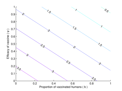
Figure 2: Simulation of the model (2.10), showing a contour plot of $\bar{R}_{0}$ as a function of proportion of vaccinated humans ($b$) and vaccine efficacy ($\psi$).

A contour plot of vaccinated reproduction number ($\bar{R}_{0}$) as a function of proportion of vaccinated humans ($b$) and vaccine efficacy ($\psi$) is shown in Fig. 2. The parameter values used to generate this diagram are given in Table 2. The contours illustrate a significant decrease in the vaccinated reproduction number, $\bar{R}_{0}$, with increasing vaccine efficacy, $\psi$, and proportion of vaccinated humans, $b$. It can be seen that very high vaccine efficacy and vaccine coverage is required to control HCV infection effectively in the population. Almost all of the susceptible individuals should have had vaccination, and vaccine efficacy must be 100% for $\bar{R}_{0}$ to be less than one, so that the spread of HCV infection is controlled effectively.

The global stability of the disease free equilibrium can be proved in the region $\Delta$ as follows.

Theorem 2.3.

For a perfect vaccine ($\psi=1$), $P_{0}$ is globally asymptotically stable in $\Delta$ whenever

$$\bar{R}_{0}\leq\displaystyle\frac{S_{0}\mu}{\Lambda}<1,$$

where

$$S_{0}=\displaystyle\frac{(1-b)\Lambda}{\mu}+\frac{\alpha b\Lambda}{\mu(\alpha+\mu)}.$$

Proof: Let

$$V=A_{1}E+A_{2}I+A_{3}T+A_{4}C_{h},$$

where

$$A_{1}=\displaystyle\frac{S_{0}\mu}{\Lambda},A_{2}=\displaystyle\frac{S_{0}K_{1}\mu}{\epsilon\Lambda},A_{3}=\displaystyle\frac{\beta_{3}S_{0}}{K_{3}},A_{4}=\displaystyle\frac{\beta_{2}S_{0}}{K_{4}}+\frac{\beta_{3}S_{0}\pi_{2}}{K_{3}K_{4}}.$$

Then,

$$\begin{array}[]{rcl}V^{\prime}&=&A_{1}E^{\prime}+A_{2}I^{\prime}+A_{3}T^{\prime}+A_{4}C_{h}^{\prime}\cr\cr&=&A_{1}\Big{[}(\beta_{1}I+\beta_{2}C_{h}+\beta_{3}T)S-K_{1}E\Big{]}+A_{2}\Big{[}\epsilon E-K_{2}I\Big{]}+A_{3}\Big{[}\pi_{1}\kappa I+\pi_{2}C_{h}-K_{3}T\Big{]}\cr\cr&&+A_{4}\Big{[}(1-\pi_{1})\kappa I-K_{4}C_{h}\Big{]}.\end{array}$$

Since, $S+E+I+T+C_{h}+V\leq\frac{\Lambda}{\mu},$ we have that

$$S\leq\frac{\Lambda}{\mu}.$$

Therefore $V^{\prime}$ becomes

$$\begin{array}[]{rcl}V^{\prime}&\leq&A_{1}\Bigr{[}(\beta_{1}I+\beta_{2}C_{h}+\beta_{3}T)\displaystyle\frac{\Lambda}{\mu}-K_{1}E\Bigr{]}+A_{2}\Big{[}\epsilon E-K_{2}I\Big{]}+A_{3}\Big{[}\pi_{1}\kappa I+\pi_{2}C_{h}-K_{3}T\Big{]}\cr\cr&&+A_{4}\Big{[}(1-\pi_{1})\kappa I-K_{4}C_{h}\Big{]}\cr\cr&=&E\Big{[}-K_{1}A_{1}+\epsilon A_{2}\Big{]}+I\Bigr{[}\beta_{1}A_{1}\displaystyle\frac{\Lambda}{\mu}-K_{2}A_{2}+\pi_{1}\kappa A_{3}+A_{4}\kappa(1-\pi_{1})\Bigr{]}+T\Bigr{[}\beta_{3}A_{1}\displaystyle\frac{\Lambda}{\mu}\cr\cr&&-K_{3}A_{3}\Bigr{]}+C_{h}\Bigr{[}\beta_{2}A_{1}\displaystyle\frac{\Lambda}{\mu}+\pi_{2}A_{3}-K_{4}A_{4}\Bigr{]}\cr\cr&=&I\Bigr{[}S_{0}\Big{(}\beta_{1}+\beta_{2}\displaystyle\frac{\kappa(1-\pi_{1})}{K_{4}}+\beta_{3}\displaystyle\frac{(\pi_{1}\kappa K_{4}+\pi_{2}\kappa(1-\pi_{1}))}{K_{3}K_{4}}\Big{)}-\displaystyle\frac{S_{0}K_{2}K_{1}\mu}{\epsilon\Lambda}\Bigr{]}\cr\cr&=&\displaystyle\frac{IK_{1}K_{2}}{\epsilon}\Bigr{[}\bar{R}_{0}-\displaystyle\frac{S_{0}\mu}{\Lambda}\Bigr{]}\leq 0,\end{array}$$

whenever

$$\bar{R}_{0}\leq\displaystyle\frac{S_{0}\mu}{\Lambda}<1.$$

Hence, $V^{\prime}\leq 0$ for $\bar{R}_{0}\leq\displaystyle\frac{S_{0}\mu}{\Lambda}$. It should also be noted that $\displaystyle\frac{S_{0}\mu}{\Lambda}=\displaystyle\frac{\frac{\Lambda}{\mu}-\frac{b\Lambda}{\alpha+\mu}}{\frac{\Lambda}{\mu}}<1.$ $V^{\prime}=0$ whenever $E=0$, $I=0$, $T=0$, $C_{h}=0$, which corresponds to the set $\{(E,I,T,C_{h}):E=I=T=C_{h}=0\}$. In this set, system (2.10) is given as

$$\begin{array}[]{rcl}\displaystyle\frac{dS}{dt}&=&(1-b)\Lambda+\alpha V-\mu S,\cr\cr\displaystyle\frac{dE}{dt}&=&\displaystyle\frac{dI}{dt}\hskip 3.41432pt=\hskip 3.41432pt\displaystyle\frac{dT}{dt}\hskip 3.41432pt=\hskip 3.41432pt\displaystyle\frac{dC_{h}}{dt}\hskip 3.41432pt=\hskip 3.41432pt0,\cr\cr\displaystyle\frac{dV}{dt}&=&b\Lambda-(\alpha+\mu)V.\end{array}$$ (2.11)

When $t\rightarrow\infty$, the solution of system (2.11) becomes

$$S=\displaystyle\frac{(1-b)\Lambda}{\mu}+\frac{\alpha b\Lambda}{\mu(\alpha+\mu)},E=0,I=0,T=0,C_{h}=0,V=\frac{b\Lambda}{\alpha+\mu}.$$

Clearly, when $t\rightarrow\infty,$ the solution to system (2.11) approaches the DFE, $P_{0}(S_{0},0,0,0,0,V_{0})$. By using LaSalle’s invariance principle (LaSalle 1976), $P_{0}$ is found to be globally asymptotically stable in $\Delta$. This result is illustrated by simulating the model (2.10) using a reasonable set of parameter values given in Table 2. The plot in Fig. 3 shows that the disease is eliminated from the population.

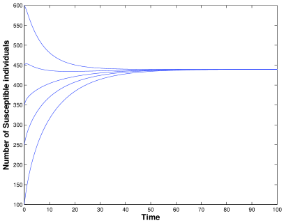
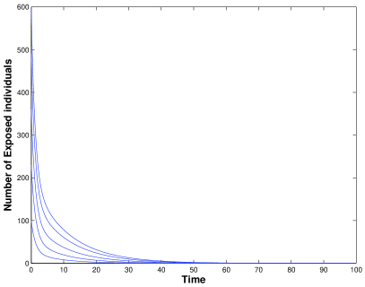
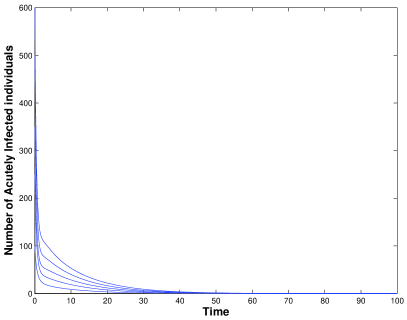
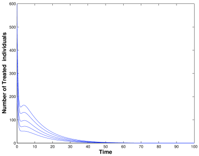
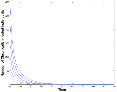
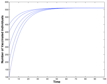
Figure 3: Simulated in MATLAB, these figures from (a) to (f) are a simulation of system (2.10), showing the total number of susceptible, exposed, acutely infected, chronically infected, treated and vaccinated individuals, respectively, as a function of time (years). Parameter values are given in Table 2, with $\psi=1$ for perfect vaccine, $\beta_{1}=0.0009,$ $\beta_{2}=0.0006,$ $\beta_{3}=0.0001$ and $\bar{R}_{0}=0.654<1.$ The numerical simulation shows that the disease is eliminated when $\bar{R}_{0}<1$ . It is assumed that the acute phase is more infectious than the chronic stage which is in turn more infectious than the treatment phase. So $\beta_{1}>\beta_{2}>\beta_{3}$.

2.3 Global stability of the endemic equilibrium

Theorem 2.4.

The endemic equilibrium $P^{\ast}(S^{\ast},E^{\ast},I^{\ast},$ $T^{\ast},C_{h}^{\ast},V^{\ast})$ of the system (2.1), with $\rho=0$ and $\sigma=0$, is globally asymptotically stable whenever it exists.

In order to prove the above theorem, we have used the method given by Li et al. (2012, 2011). At the endemic equilibrium $P^{\ast}$, with $\rho=0$ and $\sigma=0$, the following equations are satisfied:

$$\begin{array}[]{ll}0=\displaystyle(1-b)\Lambda+\alpha V^{*}-(\beta_{1}I^{*}+\beta_{2}C_{h}^{*}+\beta_{3}T^{*})S^{*}-\mu S^{*}\vskip 6.0pt plus 2.0pt minus 2.0pt\\ \displaystyle 0=(\beta_{1}I^{*}+\beta_{2}C_{h}^{*}+\beta_{3}T^{*})S^{*}+(1-\psi)(\beta_{1}I^{*}+\beta_{2}C_{h}^{*}+\beta_{3}T^{*})V^{*}-(\epsilon+\mu)E^{*}\vskip 6.0pt plus 2.0pt minus 2.0pt\\ \displaystyle 0=\epsilon E^{*}-(\kappa+\mu)I^{*}\vskip 6.0pt plus 2.0pt minus 2.0pt\\ \displaystyle 0=\pi_{1}\kappa I^{*}+\pi_{2}C_{h}^{*}-\mu T^{*}\vskip 6.0pt plus 2.0pt minus 2.0pt\\ \displaystyle 0=(1-\pi_{1})\kappa I^{*}-(\pi_{2}+\mu)C_{h}^{*}\vskip 6.0pt plus 2.0pt minus 2.0pt\\ \displaystyle 0=b\Lambda-(\alpha+\mu)V^{*}-(1-\psi)(\beta_{1}I^{*}+\beta_{2}C_{h}^{*}+\beta_{3}T^{*})V^{*}.\end{array}$$ (2.12)

Let

$$x_{1}=\displaystyle\frac{S}{S^{*}},\hskip 5.69046ptx_{2}=\displaystyle\frac{E}{E^{*}},\hskip 5.69046ptx_{3}=\displaystyle\frac{I}{I^{*}},\hskip 5.69046ptx_{4}=\displaystyle\frac{T}{T^{*}},\hskip 5.69046ptx_{5}=\displaystyle\frac{C_{h}}{C_{h}^{*}},\hskip 5.69046ptx_{6}=\displaystyle\frac{V}{V^{*}}.$$ (2.13)

Then (2.1) can be rewritten as

$$\begin{array}[]{rcl}x_{1}^{\prime}&=&x_{1}\Bigr{[}\displaystyle\frac{(1-b)\Lambda}{S^{*}}\bigg{(}\frac{1}{x_{1}}-1\bigg{)}+\frac{\alpha V^{*}}{S^{*}}\bigg{(}\frac{x_{6}}{x_{1}}-1\bigg{)}-\beta_{1}I^{*}(x_{3}-1)-\beta_{2}C_{h}^{*}(x_{5}-1)\cr\cr&&-\beta_{3}T^{*}(x_{4}-1)\Bigr{]},\cr\cr x_{2}^{\prime}&=&x_{2}\Bigr{[}\displaystyle\frac{\beta_{1}I^{*}S^{*}}{E^{*}}\bigg{(}\frac{x_{3}x_{1}}{x_{2}}-1\bigg{)}+\frac{\beta_{2}C_{h}^{*}S^{*}}{E^{*}}\bigg{(}\frac{x_{1}x_{5}}{x_{2}}-1\bigg{)}+\frac{\beta_{3}T^{*}S^{*}}{E^{*}}\bigg{(}\frac{x_{1}x_{4}}{x_{2}}-1\bigg{)}\cr\cr&&+(1-\psi)\displaystyle\frac{\beta_{1}I^{*}V^{*}}{E^{*}}\bigg{(}\frac{x_{3}x_{6}}{x_{2}}-1\bigg{)}+(1-\psi)\frac{\beta_{2}C_{h}^{*}V^{*}}{E^{*}}\bigg{(}\frac{x_{5}x_{6}}{x_{2}}-1\bigg{)}+(1-\psi)\cr\cr&&\displaystyle\frac{\beta_{3}T^{*}V^{*}}{E^{*}}\bigg{(}\frac{x_{4}x_{6}}{x_{2}}-1\bigg{)}\Bigr{]},\cr\cr x_{3}^{\prime}&=&x_{3}\Bigr{[}\displaystyle\frac{\epsilon E^{*}}{I^{*}}\bigg{(}\frac{x_{2}}{x_{3}}-1\bigg{)}\Bigr{]},\cr\cr x_{4}^{\prime}&=&x_{4}\Bigr{[}\displaystyle\frac{\pi_{1}\kappa I^{*}}{T^{*}}\bigg{(}\frac{x_{3}}{x_{4}}-1\bigg{)}+\frac{\pi_{2}C_{h}^{*}}{T^{*}}\bigg{(}\frac{x_{5}}{x_{4}}-1\bigg{)}\Bigr{]},\cr\cr\\ x_{5}^{\prime}&=&x_{5}\Bigr{[}(1-\pi_{1})\displaystyle\frac{\kappa I^{*}}{C_{h}^{*}}\big{(}\frac{x_{3}}{x_{5}}-1\big{)}\Bigr{]},\cr\cr x_{6}^{\prime}&=&x_{6}\Bigr{[}\displaystyle\frac{b\Lambda}{V^{*}}\big{(}\frac{1}{x_{6}}-1\big{)}-(1-\psi)\beta_{1}I^{*}(x_{3}-1)-(1-\psi)\beta_{2}C_{h}^{*}(x_{5}-1)-(1-\psi)\cr\cr&&\beta_{3}T^{*}(x_{4}-1)\Bigr{]}.\end{array}$$ (2.14)

The endemic equilibrium $P^{\ast}(S^{\ast},E^{\ast},I^{\ast},$ $T^{\ast},C_{h}^{\ast},V^{\ast})$ corresponds to the positive equilibrium $\bar{P}^{*}(1,1,1,1,1,1)$ of (2.14). Since, the global stability of $\bar{P}^{*}$ is the same as that of $P^{*}$, the global stability of $\bar{P}^{*}$ is described below instead of $P^{*}$. We define the Lyapunov function as follows

$$\begin{array}[]{rcl}L&=&a_{1}S^{*}(x_{1}-1-\mathrm{ln}x_{1})+a_{2}E^{*}(x_{2}-1-\mathrm{ln}x_{2})+a_{3}I^{*}(x_{3}-1-\mathrm{ln}x_{3})\cr\cr&&+a_{4}T^{*}(x_{4}-1-\mathrm{ln}x_{4})+a_{5}C_{h}^{*}(x_{5}-1-\mathrm{ln}x_{5})+a_{6}V^{*}(x_{6}-1-\mathrm{ln}x_{6}),\end{array}$$

where $a_{1},a_{2},a_{3},a_{4},a_{5}$ and $a_{6}$ are positive numbers which are to be determined. Using (2.12), the time derivative of $L$ along the solutions of system (2.1) is given as

$$\begin{array}[]{rcl}\displaystyle\frac{dL}{dt}&=&a_{1}\big{(}2(1-b)\Lambda+\alpha V^{*}-\beta_{1}I^{*}S^{*}-\beta_{2}C_{h}^{*}S^{*}-\beta_{3}T^{*}S^{*}\big{)}+a_{2}\big{(}\beta_{1}I^{*}S^{*}\cr\cr&&+\beta_{2}C_{h}^{*}S^{*}+\beta_{3}T^{*}S^{*}+(1-\psi)\beta_{1}I^{*}V^{*}+(1-\psi)\beta_{2}C_{h}^{*}V^{*}+(1-\psi)\cr\cr&&\beta_{3}T^{*}V^{*}\big{)}+a_{3}\epsilon E^{*}+a_{4}\pi_{1}\kappa I^{*}+a_{5}(1-\pi_{1})\kappa I^{*}+a_{6}\big{(}2b\Lambda-(1-\psi)\cr\cr&&\beta_{1}I^{*}V^{*}-(1-\psi)\beta_{2}C_{h}^{*}V^{*}-(1-\psi)\beta_{3}T^{*}V^{*}\big{)}-x_{1}\big{(}a_{1}(1-b)\Lambda\cr\cr&&+a_{1}\alpha V^{*}-a_{1}\beta_{1}I^{*}S^{*}-a_{1}\beta_{2}C_{h}^{*}S^{*}-a_{1}\beta_{3}T^{*}S^{*}\big{)}+x_{2}\big{(}-a_{2}\beta_{1}I^{*}S^{*}\cr\cr&&-a_{2}\beta_{2}C_{h}^{*}S^{*}-a_{2}\beta_{3}T^{*}S^{*}-a_{2}(1-\psi)\beta_{1}I^{*}V^{*}-a_{2}(1-\psi)\beta_{2}C_{h}^{*}S^{*}\cr\cr&&-a_{2}(1-\psi)\beta_{3}T^{*}V^{*}+a_{3}\epsilon E^{*}\big{)}+x_{3}\big{(}a_{1}\beta_{1}I^{*}S^{*}-a_{3}\epsilon E^{*}+a_{4}\pi_{1}\kappa I^{*}\cr\cr&&+a_{5}(1-\pi_{1}\kappa I^{*}+a_{6}(1-\psi)\beta_{1}I^{*}V^{*})\big{)}+x_{4}\big{(}a_{1}\beta_{3}T^{*}S^{*}-a_{4}\pi_{1}\kappa I^{*}\cr\cr&&-a_{4}\pi_{2}C_{h}^{*}+a_{6}(1-\psi)\beta_{3}T^{*}V^{*}\big{)}+x_{5}\big{(}a_{1}\beta_{2}C_{h}^{*}S^{*}+a_{4}\pi_{2}C_{h}^{*}-a_{5}(1\cr\cr&&-\pi_{1})\kappa I^{*}+a_{6}(1-\psi)\beta_{2}C_{h}^{*}V^{*}\big{)}-x_{6}\big{(}-a_{1}\alpha V^{*}+a_{6}b\Lambda-a_{6}(1-\psi)\cr\cr&&\beta_{1}I^{*}V^{*}-a_{6}(1-\psi)\beta_{2}C_{h}^{*}V^{*}-a_{6}(1-\psi)\beta_{3}T^{*}V^{*}\big{)}+x_{5}x_{6}\big{(}a_{2}(1-\psi)\cr\cr&&\beta_{2}C_{h}^{*}V^{*}-a_{6}(1-\psi)\beta_{2}C_{h}^{*}V^{*}\big{)}+x_{1}x_{3}\big{(}-a_{1}\beta_{1}I^{*}S^{*}+a_{2}\beta_{1}I^{*}S^{*}\big{)}\cr\cr&&+x_{1}x_{5}\big{(}-a_{1}\beta_{2}C_{h}^{*}S^{*}+a_{2}\beta_{2}C_{h}^{*}S^{*}\big{)}+x_{1}x_{4}\big{(}-a_{1}\beta_{3}T^{*}S^{*}+a_{2}\beta_{3}T^{*}S^{*}\big{)}\cr\cr&&+x_{3}x_{6}\big{(}a_{2}(1-\psi)\beta_{1}I^{*}V^{*}-a_{6}(1-\psi)\beta_{1}I^{*}V^{*}\big{)}+x_{4}x_{6}\big{(}a_{2}(1-\psi)\beta_{3}T^{*}V^{*}\cr\cr&&-a_{6}(1-\psi)\beta_{3}T^{*}V^{*}\big{)}+\displaystyle\frac{1}{x_{1}}\big{(}-a_{1}(1-b)\Lambda\big{)}+\displaystyle\frac{1}{x_{6}}\big{(}-a_{6}b\Lambda\big{)}+\frac{x_{6}}{x_{1}}\big{(}-a_{1}\alpha\cr\cr&&V^{*}\big{)}+\displaystyle\frac{x_{3}}{x_{5}}\big{(}-a_{5}(1-\pi_{1}\kappa I^{*})\big{)}+\displaystyle\frac{x_{5}}{x_{4}}\big{(}-a_{4}\pi_{2}C_{h}^{*}\big{)}+\displaystyle\frac{x_{3}}{x_{4}}\big{(}-a_{4}\pi_{1}\kappa I^{*}\big{)}+\displaystyle\frac{x_{2}}{x_{3}}\cr\cr&&\big{(}-a_{3}\epsilon E^{*}\big{)}+\displaystyle\frac{x_{3}x_{6}}{x_{2}}\big{(}-a_{2}(1-\pi)\beta_{1}I^{*}V^{*}\big{)}+\displaystyle\frac{x_{3}x_{1}}{x_{2}}\big{(}-a_{2}\beta_{1}I^{*}S^{*}\big{)}+\displaystyle\frac{x_{5}x_{1}}{x_{2}}\cr\cr&&\big{(}-a_{2}\beta_{2}C_{h}^{*}S^{*}\big{)}+\displaystyle\frac{x_{1}x_{4}}{x_{2}}\big{(}-a_{2}\beta_{3}T^{*}S^{*}\big{)}+\displaystyle\frac{x_{4}x_{6}}{x_{2}}\big{(}-a_{2}(1-\pi)\beta_{3}T^{*}V^{*}\big{)}\cr\cr&&+\displaystyle\frac{x_{5}x_{6}}{x_{2}}\big{(}-a_{2}(1-\pi)\beta_{2}C_{h}^{*}V^{*}\big{)}\cr\cr&=:&F(x_{1},x_{2},x_{3},x_{4},x_{5},x_{6}).\end{array}$$

We define the function $H=\sum_{i=1}^{14}P_{i}$, where $P_{i}(i=1,2,...,14)$ is given as

$$\begin{array}[]{ll}\displaystyle P_{1}=b_{1}\Big{(}2-x_{1}-\displaystyle\frac{1}{x_{1}}\Big{)},\vspace{.7em}\\ \displaystyle P_{2}=b_{2}\Big{(}2-x_{6}-\displaystyle\frac{1}{x_{6}}\Big{)},\vspace{.7em}\\ \displaystyle P_{3}=b_{3}\Big{(}3-x_{1}-\displaystyle\frac{1}{x_{6}}-\displaystyle\frac{x_{6}}{x_{1}}\Big{)},\vspace{.7em}\\ \displaystyle P_{4}=b_{4}\Big{(}3-\displaystyle\frac{1}{x_{1}}-\displaystyle\frac{x_{1}x_{3}}{x_{2}}-\displaystyle\frac{x_{2}}{x_{3}}\Big{)},\vspace{.5em}\\ \displaystyle P_{5}=b_{5}\Big{(}4-\displaystyle\frac{1}{x_{1}}-\displaystyle\frac{x_{1}x_{4}}{x_{2}}-\displaystyle\frac{x_{3}}{x_{4}}-\displaystyle\frac{x_{2}}{x_{3}}\Big{)},\vspace{.7em}\\ \displaystyle P_{6}=b_{6}\Big{(}4-\displaystyle\frac{1}{x_{1}}-\displaystyle\frac{x_{1}x_{5}}{x_{2}}-\displaystyle\frac{x_{3}}{x_{5}}-\displaystyle\frac{x_{2}}{x_{3}}\Big{)},\vspace{.7em}\\ \displaystyle P_{7}=b_{7}\Big{(}5-\displaystyle\frac{1}{x_{1}}-\displaystyle\frac{x_{1}x_{4}}{x_{2}}-\displaystyle\frac{x_{5}}{x_{4}}-\displaystyle\frac{x_{2}}{x_{3}}-\frac{x_{3}}{x_{5}}\Big{)},\vspace{.7em}\\ \displaystyle P_{8}=b_{8}\Big{(}3-\displaystyle\frac{1}{x_{6}}-\displaystyle\frac{x_{3}x_{6}}{x_{2}}-\displaystyle\frac{x_{2}}{x_{3}}\Big{)},\vspace{.5em}\\ \displaystyle P_{9}=b_{9}\Big{(}4-\displaystyle\frac{1}{x_{6}}-\displaystyle\frac{x_{4}x_{6}}{x_{2}}-\displaystyle\frac{x_{3}}{x_{4}}-\displaystyle\frac{x_{2}}{x_{3}}\Big{)},\vspace{.7em}\\ \displaystyle P_{10}=b_{10}\Big{(}5-\displaystyle\frac{1}{x_{6}}-\displaystyle\frac{x_{4}x_{6}}{x_{2}}-\displaystyle\frac{x_{5}}{x_{4}}-\displaystyle\frac{x_{2}}{x_{3}}-\frac{x_{3}}{x_{5}}\Big{)},\vspace{.7em}\\ \displaystyle P_{11}=b_{11}\Big{(}4-\displaystyle\frac{1}{x_{6}}-\displaystyle\frac{x_{5}x_{6}}{x_{2}}-\displaystyle\frac{x_{3}}{x_{5}}-\displaystyle\frac{x_{2}}{x_{3}}\Big{)},\vspace{.7em}\\ \displaystyle P_{12}=b_{12}\Big{(}4-\displaystyle\frac{1}{x_{6}}-\displaystyle\frac{x_{1}x_{3}}{x_{2}}-\displaystyle\frac{x_{6}}{x_{1}}-\displaystyle\frac{x_{2}}{x_{3}}\Big{)},\vspace{.7em}\\ \displaystyle P_{13}=b_{13}\Big{(}5-\displaystyle\frac{1}{x_{6}}-\displaystyle\frac{x_{1}x_{5}}{x_{2}}-\displaystyle\frac{x_{6}}{x_{1}}-\displaystyle\frac{x_{2}}{x_{3}}-\frac{x_{3}}{x_{5}}\Big{)},\vspace{.7em}\\ \displaystyle P_{14}=b_{14}\Big{(}5-\displaystyle\frac{1}{x_{6}}-\displaystyle\frac{x_{1}x_{4}}{x_{2}}-\displaystyle\frac{x_{6}}{x_{1}}-\displaystyle\frac{x_{2}}{x_{3}}-\frac{x_{3}}{x_{4}}\Big{)}.\vspace{.7em}\end{array}$$ (2.15)

To determine all the coefficients, ( $a_{i}>0$ $(i=1,2,...,6)$, $b_{i}\geq 0$ $(i=1,2,...,14)$ ) we let $F(x_{1},x_{2},x_{3},x_{4},x_{5},x_{6})$ = $H$. Comparing coefficients of $F$ and $H$, we see that the terms $x_{2},~{}x_{4},~{}x_{5},~{}x_{5}x_{6},~{}x_{1}x_{3},~{}x_{1}x_{5},~{}x_{1}x_{4},~{}x_{3}x_{6}$, and $x_{4}x_{6}$ of $F$ do not appear in $H$. Hence their coefficients will be equal to zero. We solve the resulting equations to obtain

$$a_{1}=a_{2}=a_{6}=1,$$

$$a_{3}=\displaystyle\frac{\epsilon+\mu}{\epsilon},$$

$$a_{4}=\displaystyle\frac{\beta_{3}S^{*}+(1-\psi)\beta_{3}V^{*}}{\mu},$$

$$a_{5}=\displaystyle\frac{\big{(}S^{*}+(1-\psi)V^{*}\big{)}\big{(}\beta_{2}+\frac{\beta_{3}\pi_{2}}{\mu}\big{)}}{\pi_{2}+\mu}.$$

Substituting these values into $L^{\prime}=F(x_{1},x_{2},x_{3},x_{4},x_{5},x_{6})$, and using equations (2.12) gives

$$\begin{array}[]{rcl}&&F(x_{1},x_{2},x_{3},x_{4},x_{5},x_{6})=\Big{(}2\Lambda+\alpha V^{*}+(\epsilon+\mu)E^{*}+\beta_{3}\big{(}S^{*}+(1-\psi)V^{*}\big{)}T^{*}\cr\cr&&+\big{(}S^{*}+(1-\psi)V^{*}\big{)}\big{(}\beta_{2}+\displaystyle\frac{\beta_{3}\pi_{2}}{\mu}\big{)}C_{h}^{*}\Big{)}-x_{1}\big{(}\mu S^{*}\big{)}-x_{6}\big{(}\mu V^{*}\big{)}-\displaystyle\frac{1}{x_{1}}\big{(}(1-b)\Lambda\big{)}\cr\cr&&-\displaystyle\frac{1}{x_{6}}\big{(}b\Lambda\big{)}-\frac{x_{6}}{x_{1}}\big{(}\alpha V^{*}\big{)}-\frac{x_{3}}{x_{5}}\Big{(}\big{(}S^{*}+(1-\psi)V^{*}\big{)}\big{(}\beta_{2}+\displaystyle\frac{\beta_{3}\pi_{2}}{\mu}\big{)}C_{h}^{*}\Big{)}-\displaystyle\frac{x_{5}}{x_{4}}\Big{(}\displaystyle\frac{\beta_{3}}{\mu}\cr\cr&&\big{(}S^{*}+(1-\psi)V^{*}\big{)}\pi_{2}C_{h}^{*}\Big{)}-\displaystyle\frac{x_{3}}{x_{4}}\Big{(}\displaystyle\frac{\beta_{3}}{\mu}\big{(}S^{*}+(1-\psi)V^{*}\big{)}\pi_{1}\kappa I^{*}\Big{)}-\displaystyle\frac{x_{2}}{x_{3}}\Big{(}(\epsilon+\mu)E^{*}\Big{)}\cr\cr&&-\displaystyle\frac{x_{3}x_{6}}{x_{2}}\big{(}(1-\psi)\beta_{1}I^{*}V^{*}\big{)}-\displaystyle\frac{x_{1}x_{3}}{x_{2}}\big{(}\beta_{1}I^{*}S^{*}\big{)}-\displaystyle\frac{x_{1}x_{5}}{x_{2}}\big{(}\beta_{2}C_{h}^{*}S^{*}\big{)}-\displaystyle\frac{x_{1}x_{4}}{x_{2}}\big{(}\beta_{3}T^{*}S^{*}\big{)}\cr\cr&&-\displaystyle\frac{x_{4}x_{6}}{x_{2}}\big{(}(1-\psi)\beta_{3}T^{*}V^{*}\big{)}-\displaystyle\frac{x_{5}x_{6}}{x_{2}}\big{(}(1-\psi)\beta_{2}C_{h}^{*}V^{*}\big{)}.\end{array}$$

Comparing the remaining coefficients of $F$ and $H$ gives

$$\begin{array}[]{ll}b_{1}=\mu S^{*}-\alpha V^{*}+b_{12}+b_{13}+b_{14},{}{}\vspace{.5em}\\ b_{2}=\mu V^{*}\geq 0,{}{}\vspace{.5em}\\ b_{3}=\alpha V^{*}-b_{12}-b_{13}-b_{14},{}{}\vspace{.5em}\\ b_{4}=\beta_{1}I^{*}S^{*}-b_{12},{}{}\vspace{.5em}\\ b_{5}=\beta_{3}T^{*}S^{*}-\displaystyle\frac{\beta_{3}}{\mu}\big{(}S^{*}+(1-\psi)V^{*}\big{)}\pi_{2}C_{h}^{*}+b_{10}-b_{14},{}{}\vspace{.5em}\\ b_{6}=\beta_{2}C_{h}^{*}S^{*}-b_{13},{}{}\vspace{.5em}\\ b_{7}=\displaystyle\frac{\beta_{3}}{\mu}\big{(}S^{*}+(1-\psi)V^{*}\big{)}\pi_{2}C_{h}^{*}-b_{10},{}{}\vspace{.5em}\\ b_{8}=(1-\psi)\beta_{1}I^{*}V^{*}\geq 0,{}{}\vspace{.5em}\\ b_{9}=(1-\psi)\beta_{3}T^{*}V^{*}-b_{10},{}{}\vspace{.5em}\\ b_{11}=(1-\psi)\beta_{2}C_{h}^{*}V^{*}\geq 0.\vspace{.5em}\end{array}$$ (2.16)

To assure that $b_{1},b_{3},b_{4},b_{5},b_{6},b_{7}$ and $b_{9}$ are non negative, $b_{10},b_{12},b_{13},b_{14}$ must satisfy the following inequalities

$$\begin{array}[]{ll}\displaystyle\alpha V^{*}-\mu S^{*}\leq b_{12}+b_{13}+b_{14}\leq\alpha V^{*},\vspace{.5em}\\ \displaystyle b_{10}\leq\min\Big{(}(1-\psi)\beta_{3}T^{*}V^{*},\displaystyle\frac{\beta_{3}}{\mu}\big{(}S^{*}+(1-\psi)V^{*}\big{)}\pi_{2}C_{h}^{*}\Big{)},\vspace{.5em}\\ \displaystyle b_{14}-b_{10}\leq\beta_{3}T^{*}S^{*}-\displaystyle\frac{\beta_{3}}{\mu}\big{(}S^{*}+(1-\psi)V^{*}\big{)}\pi_{2}C_{h}^{*},\vspace{.5em}\\ \displaystyle b_{12}\leq\beta_{1}I^{*}S^{*},\vspace{.5em}b_{13}\leq\beta_{2}C_{h}^{*}S^{*}\vspace{.5em}.\end{array}$$ (2.17)

Finally, using equations (2.12), the equality for the constant terms between $F(x_{1},x_{2},x_{3},x_{4},x_{5},x_{6})$ and $H$ can easily be verified.

The constrained conditions in (2.17) show that the available values of $b_{10},b_{12},b_{13},$ and $b_{14}$ are not unique. Since, $b_{1},b_{3},b_{4},b_{5},b_{6},b_{7}$ and $b_{9}$ depend on $b_{10},b_{12},b_{13},$ and $b_{14}$, their values will also be non unique. Using inequalities in (2.17), we can assign different values to $b_{i}(i=1,3,...14,i\neq 2,8,11)$, and hence $H$ can have different forms in following three subregions

Case 1: $\mu S>\alpha V,~{}~{}\displaystyle\frac{\beta_{3}}{\mu}\big{(}S^{*}+(1-\psi)V^{*}\big{)}\pi_{2}C_{h}^{*}\leq(1-\psi)\beta_{3}T^{*}V^{*}.$

For Case 1, using equations (2.16) and (2.17), choose $b_{1}=\mu S^{*}-\alpha V^{*}$, $b_{3}=\alpha V^{*}$, $b_{4}=\beta_{1}I^{*}S^{*}$, $b_{5}=\beta_{3}T^{*}S^{*}$, $b_{6}=\beta_{2}C_{h}^{*}S^{*}$, $b_{7}=0$, $b_{9}=(1-\psi)\beta_{3}T^{*}V^{*}\vspace{.2em}-\displaystyle\frac{\beta_{3}}{\mu}\big{(}S^{*}+(1-\psi)V^{*}\big{)}\pi_{2}C_{h}^{*}$, $b_{10}=\displaystyle\frac{\beta_{3}}{\mu}\big{(}S^{*}+(1-\psi)V^{*}\big{)}\pi_{2}C_{h}^{*}$, $b_{12}=0$, $b_{13}=0$ and $b_{14}=0$.

Using these values, and the values of $b_{2},b_{8}$ and $b_{11}$, the function $F(x_{1},x_{2},x_{3},x_{4},x_{5},x_{6})$ becomes

$F(x_{1},x_{2},x_{3},x_{4},x_{5},x_{6})=$

$$\begin{array}[]{ll}\displaystyle(\mu S^{*}-\alpha V^{*})\Big{(}2-x_{1}-\displaystyle\frac{1}{x_{1}}\Big{)}+\mu V^{*}\Big{(}2-x_{6}-\displaystyle\frac{1}{x_{6}}\Big{)}\displaystyle+\alpha V^{*}\Big{(}3-x_{1}-\displaystyle\frac{1}{x_{6}}\vspace{.2cm}\\ -\displaystyle\frac{x_{6}}{x_{1}}\Big{)}\displaystyle+\beta_{1}I^{*}S^{*}\Big{(}3-\displaystyle\frac{1}{x_{1}}-\displaystyle\frac{x_{2}}{x_{3}}-\displaystyle\frac{x_{1}x_{3}}{x_{2}}\Big{)}\displaystyle+\beta_{3}T^{*}S^{*}\Big{(}4-\displaystyle\frac{1}{x_{1}}-\displaystyle\frac{x_{2}}{x_{3}}-\displaystyle\frac{x_{1}x_{4}}{x_{2}}\vspace{.2cm}\\ -\displaystyle\frac{x_{3}}{x_{4}}\Big{)}\displaystyle+\beta_{2}C_{h}^{*}S^{*}\Big{(}4-\displaystyle\frac{1}{x_{1}}-\displaystyle\frac{x_{2}}{x_{3}}-\displaystyle\frac{x_{1}x_{5}}{x_{2}}-\displaystyle\frac{x_{3}}{x_{5}}\Big{)}\displaystyle+(1-\psi)\beta_{1}I^{*}V^{*}\Big{(}3-\displaystyle\frac{1}{x_{6}}\vspace{.2cm}\\ -\displaystyle\frac{x_{2}}{x_{3}}-\displaystyle\frac{x_{3}x_{6}}{x_{2}}\Big{)}+\Big{(}(1-\psi)\beta_{3}T^{*}V^{*}\displaystyle-\displaystyle\frac{\beta_{3}}{\mu}\big{(}S^{*}+(1-\psi)V^{*}\big{)}\pi_{2}C_{h}^{*}\Big{)}\Big{(}4-\displaystyle\frac{1}{x_{6}}\vspace{.2cm}\\ -\displaystyle\frac{x_{2}}{x_{3}}-\displaystyle\frac{x_{4}x_{6}}{x_{2}}-\displaystyle\frac{x_{3}}{x_{4}}\Big{)}\displaystyle+\displaystyle\frac{\beta_{3}}{\mu}\big{(}S^{*}+(1-\psi)V^{*}\big{)}\pi_{2}C_{h}^{*}\Big{(}5-\displaystyle\frac{1}{x_{6}}\displaystyle-\displaystyle\frac{x_{2}}{x_{3}}-\displaystyle\frac{x_{4}x_{6}}{x_{2}}\vspace{.2cm}\\ -\displaystyle\frac{x_{3}}{x_{5}}-\displaystyle\frac{x_{5}}{x_{4}}\Big{)}\displaystyle+(1-\psi)\beta_{2}C_{h}^{*}V^{*}\Big{(}4-\displaystyle\frac{1}{x_{6}}-\displaystyle\frac{x_{2}}{x_{3}}-\displaystyle\frac{x_{5}x_{6}}{x_{2}}-\displaystyle\frac{x_{3}}{x_{5}}\Big{)}.\end{array}$$

Case 2: $\mu S=\alpha V,~{}~{}\displaystyle\frac{\beta_{3}}{\mu}\big{(}S^{*}+(1-\psi)V^{*}\big{)}\pi_{2}C_{h}^{*}\geq(1-\psi)\beta_{3}T^{*}V^{*}.$

For Case 2, using equations (2.16) and (2.17), choose $b_{1}=0$, $b_{3}=\alpha V^{*}$, $b_{4}=\beta_{1}I^{*}S^{*}$, $b_{5}=\beta_{3}\big{(}S^{*}+(1-\psi)V^{*}\big{)}\displaystyle\frac{\pi_{1}\kappa I^{*}}{\mu}$, $b_{6}=\beta_{2}C_{h}^{*}S^{*}$, $b_{7}=\displaystyle\frac{\beta_{3}}{\mu}\big{(}S^{*}+(1-\psi)V^{*}\big{)}\pi_{2}C_{h}^{*}-(1-\psi)\beta_{3}T^{*}V^{*}$, $b_{9}=0$, $b_{10}=(1-\psi)\beta_{3}T^{*}V^{*}$, $b_{12}=0$, $b_{13}=0$ and $b_{14}=0$.

Using the above values, and the values of $b_{2},b_{8}$ and $b_{11}$, the function $F(x_{1},x_{2},x_{3},x_{4},x_{5},x_{6})$ becomes

$F(x_{1},x_{2},x_{3},x_{4},x_{5},x_{6})$=

$$\begin{array}[]{ll}\mu V^{*}\Big{(}2-x_{6}-\displaystyle\frac{1}{x_{6}}\Big{)}+\alpha V^{*}\Big{(}3-x_{1}-\displaystyle\frac{1}{x_{6}}-\displaystyle\frac{x_{6}}{x_{1}}\Big{)}\displaystyle+\beta_{1}I^{*}S^{*}\Big{(}3-\displaystyle\frac{1}{x_{1}}-\displaystyle\frac{x_{2}}{x_{3}}-\displaystyle\frac{x_{1}x_{3}}{x_{2}}\Big{)}\vspace{.2cm}\\ \displaystyle+\beta_{3}\big{(}S^{*}+(1-\psi)V^{*}\big{)}\displaystyle\frac{\pi_{1}\kappa I^{*}}{\mu}\Big{(}4-\displaystyle\frac{1}{x_{1}}-\displaystyle\frac{x_{2}}{x_{3}}-\displaystyle\frac{x_{1}x_{4}}{x_{2}}-\displaystyle\frac{x_{3}}{x_{4}}\Big{)}\displaystyle+\beta_{2}C_{h}^{*}S^{*}\Big{(}4-\displaystyle\frac{1}{x_{1}}-\displaystyle\frac{x_{2}}{x_{3}}\vspace{.2cm}\\ -\displaystyle\frac{x_{1}x_{5}}{x_{2}}-\displaystyle\frac{x_{3}}{x_{5}}\Big{)}\displaystyle+\big{(}\displaystyle\frac{\beta_{3}}{\mu}\big{(}S^{*}+(1-\psi)V^{*}\big{)}\pi_{2}C_{h}^{*}-(1-\psi)\beta_{3}T^{*}V^{*}\big{)}\displaystyle\Big{(}5-\displaystyle\frac{1}{x_{1}}-\displaystyle\frac{x_{2}}{x_{3}}-\displaystyle\frac{x_{1}x_{4}}{x_{2}}\vspace{.2cm}\\ -\displaystyle\frac{x_{3}}{x_{5}}-\displaystyle\frac{x_{5}}{x_{4}}\Big{)}\displaystyle+(1-\psi)\beta_{1}I^{*}V^{*}\Big{(}3-\displaystyle\frac{1}{x_{6}}-\displaystyle\frac{x_{2}}{x_{3}}-\displaystyle\frac{x_{3}x_{6}}{x_{2}}\Big{)}\displaystyle+(1-\psi)\beta_{3}T^{*}V^{*}\Big{(}5-\displaystyle\frac{1}{x_{6}}-\displaystyle\frac{x_{2}}{x_{3}}\vspace{.2cm}\\ -\displaystyle\frac{x_{4}x_{6}}{x_{2}}-\displaystyle\frac{x_{3}}{x_{5}}-\displaystyle\frac{x_{5}}{x_{4}}\Big{)}\displaystyle+(1-\psi)\beta_{2}C_{h}^{*}V^{*}\Big{(}4-\displaystyle\frac{1}{x_{6}}-\displaystyle\frac{x_{2}}{x_{3}}-\displaystyle\frac{x_{5}x_{6}}{x_{2}}-\displaystyle\frac{x_{3}}{x_{5}}\Big{)}.\end{array}$$

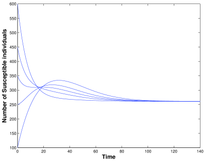
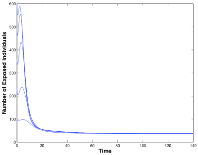
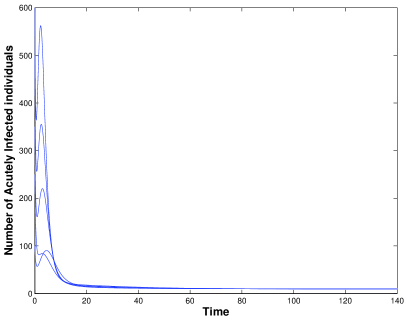
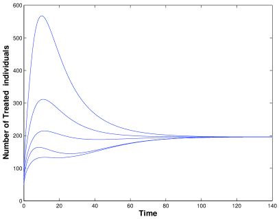
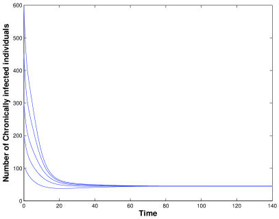
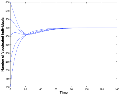
Figure 4: Simulation (in MATLAB) of system (2.1), showing the total number of susceptible, exposed, acutely infected, chronically infected, treated and vaccinated individuals as a function of time (years) when $R_{0}>1$. Parameter values are given in Table 2, with $\psi=0.6$, $\rho=0$, $\sigma=0$, $\beta_{1}=0.0009,$ $\beta_{2}=0.0006,$ and $\beta_{3}=0.0001$. The numerical simulation shows that the disease persists when $R_{0}>1$.

Case 3: $\mu S<\alpha V,~{}~{}\displaystyle\frac{\beta_{3}}{\mu}\big{(}S^{*}+(1-\psi)V^{*}\big{)}\pi_{2}C_{h}^{*}\geq(1-\psi)\beta_{3}T^{*}V^{*}.$

For Case 3, using equations (2.16) and (2.17), we assume that $\alpha V^{*}\leq\beta_{3}\big{(}S^{*}+(1-\psi)V^{*}\big{)}\displaystyle\frac{\pi_{1}\kappa I^{*}}{\mu}$ and choose $b_{1}=\mu S^{*}$, $b_{3}=0$, $b_{4}=\beta_{1}I^{*}S^{*}$, $b_{5}=\beta_{3}\big{(}S^{*}+(1-\psi)V^{*}\big{)}\displaystyle\frac{\pi_{1}\kappa I^{*}}{\mu}-\alpha V^{*}$, $b_{6}=\beta_{2}C_{h}^{*}S^{*}$, $b_{7}=\displaystyle\frac{\beta_{3}}{\mu}\big{(}S^{*}+(1-\psi)V^{*}\big{)}\pi_{2}C_{h}^{*}-(1-\psi)\beta_{3}T^{*}V^{*}$, $b_{9}=0$, $b_{10}=(1-\psi)\beta_{3}T^{*}V^{*}$, $b_{12}=0$, $b_{13}=0$ and $b_{14}=\alpha V^{*}$.

Using the above values, and the values of $b_{2},b_{8}$ and $b_{11}$, the function $F(x_{1},x_{2},x_{3},x_{4},x_{5},x_{6})$ becomes

$F(x_{1},x_{2},x_{3},x_{4},x_{5},x_{6})$=

$$\begin{array}[]{lll}\mu S^{*}\Big{(}2-x_{1}-\displaystyle\frac{1}{x_{1}}\Big{)}+\mu V^{*}\Big{(}2-x_{6}-\displaystyle\frac{1}{x_{6}}\Big{)}+\beta_{1}I^{*}S^{*}\Big{(}3-\displaystyle\frac{1}{x_{1}}-\displaystyle\frac{x_{2}}{x_{3}}-\displaystyle\frac{x_{1}x_{3}}{x_{2}}\Big{)}\vspace{.2cm}\\ +\Big{(}\beta_{3}\big{(}S^{*}+(1-\psi)V^{*}\big{)}\displaystyle\frac{\pi_{1}\kappa I^{*}}{\mu}-\alpha V^{*}\Big{)}\Big{(}4-\displaystyle\frac{1}{x_{1}}-\displaystyle\frac{x_{2}}{x_{3}}-\displaystyle\frac{x_{1}x_{4}}{x_{2}}-\displaystyle\frac{x_{3}}{x_{4}}\Big{)}+\beta_{2}C_{h}^{*}S^{*}\vspace{.2cm}\\ \Big{(}4-\displaystyle\frac{1}{x_{1}}-\displaystyle\frac{x_{2}}{x_{3}}-\displaystyle\frac{x_{1}x_{5}}{x_{2}}-\displaystyle\frac{x_{3}}{x_{5}}\Big{)}+\displaystyle\frac{\beta_{3}}{\mu}\big{(}S^{*}+(1-\psi)V^{*}\big{)}\pi_{2}C_{h}^{*}-(1-\psi)\beta_{3}T^{*}V^{*}\vspace{.2cm}\\ \Big{(}5-\displaystyle\frac{1}{x_{1}}-\displaystyle\frac{x_{2}}{x_{3}}-\displaystyle\frac{x_{1}x_{4}}{x_{2}}-\displaystyle\frac{x_{5}}{x_{4}}-\displaystyle\frac{x_{3}}{x_{5}}\Big{)}+(1-\psi)\beta_{1}I^{*}V^{*}\Big{(}3-\displaystyle\frac{1}{x_{6}}-\displaystyle\frac{x_{2}}{x_{3}}-\displaystyle\frac{x_{3}x_{6}}{x_{2}}\Big{)}\vspace{.2cm}\\ +(1-\psi)\beta_{3}T^{*}V^{*}\Big{(}5-\displaystyle\frac{1}{x_{6}}-\displaystyle\frac{x_{2}}{x_{3}}-\displaystyle\frac{x_{4}x_{6}}{x_{2}}-\displaystyle\frac{x_{3}}{x_{5}}-\displaystyle\frac{x_{5}}{x_{4}}\Big{)}+(1-\psi)\beta_{2}C_{h}^{*}V^{*}\Big{(}4-\vspace{.2cm}\\ \displaystyle\frac{1}{x_{6}}-\displaystyle\frac{x_{2}}{x_{3}}-\displaystyle\frac{x_{5}x_{6}}{x_{2}}-\displaystyle\frac{x_{3}}{x_{5}}\Big{)}+\alpha V^{*}\Big{(}5-\displaystyle\frac{1}{x_{6}}-\displaystyle\frac{x_{2}}{x_{3}}-\displaystyle\frac{x_{1}x_{4}}{x_{2}}-\displaystyle\frac{x_{3}}{x_{4}}-\displaystyle\frac{x_{6}}{x_{1}}\Big{)}.\end{array}$$

Since, the arithmetic mean is greater than or equal to the geometric mean,
$F(x_{1},x_{2},x_{3},x_{4},x_{5},x_{6})$ $\leq 0$ in each of the above three cases. The equality holds only when $x_{1}=x_{6}=1$, and $x_{2}=x_{3}=x_{4}=x_{5}$, i.e. $\{(x_{1},x_{2},x_{3},x_{4},x_{5},x_{6})\in\Delta:F(x_{1},x_{2},x_{3},x_{4},x_{5},x_{6})=0\}=\{(x_{1},x_{2},x_{3},x_{4},x_{5},x_{6}):x_{1}=x_{6}=1,x_{2}=x_{3}=x_{4}=x_{5}\}$.This corresponds to the set $\Delta^{\prime}=\{(S,E,I,T,C_{h},V):S=S^{*},V=V^{*},E/E^{*}=I/I^{*}=T/T^{*}=C_{h}/C_{h}^{*}\}\in\Delta$. Hence, the maximum invariant set of (2.1) on the set $\Delta^{\prime}$ is the singleton $\{P^{*}\}$. Therefore, by LaSalle’s Invariance principle, the endemic equilibrium $P^{*}$ is globally stable in $\Delta$ when $\rho=0$ and $\sigma=0$. This result is illustrated by simulating the model in equation (2.1) using a reasonable set of parameter values given in Table 2. The plot shows that the disease persists in the population (Fig. 4).

3 Conclusions

This paper presents a deterministic model for the transmission dynamics of Hepatitis C virus infection. The formulated model, realistically, allows HCV transmission by acutely and chronically infected individuals. Most importantly, the model includes a compartment of vaccinated individuals, and considers the effect of a waning vaccine on the transfer of individuals from one compartment to another. The model was rigorously analyzed to gain insights into its qualitative dynamics. We obtained the following results:

1. The model has a locally stable disease free equilibrium whenever the associated reproduction number is less than unity.

2. The model exhibits the phenomenon of backward bifurcation, suggesting a case where stable disease-free equilibrium co-exists with a stable endemic equilibrium whenever the basic reproductive number is less than unity.

3. Using an imperfect Hepatitis C vaccine would have no positive epidemiological impact to reduce disease burden in the community.

4. Using a perfect vaccine can result in effective elimination of HCV infection in a community, that is, the efficacy of the vaccine should be $100\%$ for complete removal of the disease.

References

- [1] Allen LJS (2007) An Introduction to Mathematical Biology. Pearson Prentice Hall, New Jersey
- [2] Castillo-Chavez C, Song B (2004) Dynamical model of tuberculosis and their applications. Math Biosci Eng 1:361-404
- [3] Chen JY, Li F (2006) Development of hepatitis C virus vaccine using hepatitis B core antigen as immuno-carrier. World J Gastroentero 12:7774-7778
- [4] Cotran RS, Kumar V, Robbins SL (1994) Pathologic basis of disease. Saunders, Philadelphia
- [5] Dahari H, Feliu A, Garcia-Retortillo M, Forns X, Neumann AU (2005) Second hepatitis C replication compartment indicated by viral dynamics during liver transplantation. J Hepatol 42:491-498
- [6] Das P, Mukherjee D, Sarakar J (2005) Analysis of a disease transmission model of hepatitis C. J Biol Syst 6:331-339
- [7] Di Bisceglie AM (2000) Natural history of hepatitis C: its impact on clinical management. Hepatology 31:1014-1018
- [8] Driessche P, Watmough J (2002) Reproduction numbers and sub-threshold endemic equilibria for compartmental models of disease transmission. Math Biosci 180:29-48
- [9] Elbasha EH (2013) Model for hepatitis C virus transmissions. Math Biosci Eng 10:1045-1065
- [10] Garba SM, Gumel AB, Abu Bakar MR (2008) Backward bifurcations in dengue transmission dynamics. Math Biosci 215:11-25
- [11] Jager J, Limburg W, Kretzschmar M, Postma M, Wiessing L (2004) Hepatitis C and injecting drug use: impact, costs and policy options. Monograph, EMCDDA Lisbon
- [12] LaSalle JP (1976) The stability of dynamical systems. Society for Industrial and Applied Mathematics, SIAM Philadelphia
- [13] Li J, Xiao Y, Zhang F, Yang Y (2012) An algebraic approach to proving the global stability of a class of epidemic models. Nonlinear Anal-Real 13:2006-2016
- [14] Li J, Yang Y, Zhou Y (2011) Global stability of an epidemic model with latent stage and vaccination. Nonlinear Anal-Real 12:2163-2173
- [15] Lozano R, Naghavi M, Foreman K, Lim S, Shibuya K, Aboyans V, Abraham J (1990) Hepatitis C factsheet no.164. World Health Organization. http://www.who.int/mediacentre/factsheets/fs164/en/. Accessed 10 December 2012
- [16] Martcheva M, Castillo-Chavez C (2003) Diseases with chronic stage in a population with varying size. Math Biosci 182:1-25
- [17] Martin NK, Vickerman P, Foster GR, Hutchinson SJ, Goldberg DJ, Hickman M (2011) Can antiviral therapy for hepatitis C reduce the prevalence of HCV among injecting drug user populations? A modeling analysis of its prevention utility. J Hepatol 54:1137-1144
- [18] Martin NK, Vickerman P, Hickman M (2011) Mathematical modelling of hepatitis C treatment for injecting drug users. J Theor Biol 274:58-66
- [19] Qesmi R, Wu J, Heffernan JM (2010) Influence of backward bifurcation in a model of hepatitis B and C viruses. Math Biosci 224:118-125
- [20] Safi MA, Gumel AB (2011) Mathematical analysis of a disease transmission model with quarantine, isolation and an imperfect vaccine. Comput Math Appl 61:3044-3070
- [21] Zeiler I, Langlands T, Murray JM, Ritter A (2010) Optimal targeting of Hepatitis C virus treatment among injecting drug users to those not enrolled in methadone maintenance programs. Drug Alcohol Depen 110:228-233
- [22] Zhang S, Zhou Y (2012) The analysis and application of an HBV model. Appl Math Model 36:1302-1312