Shaping electron wave functions in a carbon nanotube with a parallel magnetic field

Abstract

A magnetic field, through its vector potential, usually causes measurable changes in the electron wave function only in the direction transverse to the field. Here we demonstrate experimentally and theoretically that in carbon nanotube quantum dots, combining cylindrical topology and bipartite hexagonal lattice, a magnetic field along the nanotube axis impacts also the longitudinal profile of the electronic states. With the high (up to 17 T) magnetic fields in our experiment the wave functions can be tuned all the way from “half-wave resonator” shape, with nodes at both ends, to “quarter-wave resonator” shape, with an antinode at one end. This in turn causes a distinct dependence of the conductance on the magnetic field. Our results demonstrate a new strategy for the control of wave functions using magnetic fields in quantum systems with nontrivial lattice and topology.

As first noticed by Aharonov and Bohm Aharonov and Bohm (1959), when a charged quantum particle travels in a finite electromagnetic potential, its wave function acquires a phase whose magnitude depends on the travelled path. For particles with electric charge $q$ moving along a closed path, the phase shift $\varphi_{AB}=q\Phi_{B}/h$, known as Aharonov-Bohm shift, is expressed in terms of the magnetic flux $\Phi_{B}$ across the enclosed area. Because $\Phi_{B}$ depends only on the magnitude of the magnetic field component normal to this area’s surface, the phase is acquired along directions transverse to the magnetic field, see Fig. 1(a). In mesoscopic rings or tubular structures pierced by a magnetic field, the phase changes the quantization condition for the tangential part of the electronic wave vector by $k_{\perp}\rightarrow k_{\perp}+\varphi_{AB}/r$ (with $r$ the radius of the ring or tubulus) and is at the basis of remarkable quantum interference phenomena Webb et al. (1985). However, as the perpendicular components of the magnetic vector potential commute with the parallel component of the momentum, a parallel magnetic field is not expected to affect the wave function along the field.

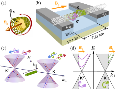
Figure 1: (a) Electrons circulating in closed orbits acquire an Aharonov-Bohm phase proportional to the enclosed magnetic flux. (b) Schematic of a suspended CNT device with its embedded quantum dot (shaded green) and a magnetic field parallel to the nanotube. (c) Dirac cones of the graphene dispersion relation. Blue and red lines indicate the lowermost transverse subbands forming in a CNT. Spin degeneracy is lifted by the spin-orbit coupling. Quantized $k_{\parallel}$ values due to a finite CNT length are marked with dots; $B_{\parallel}=0$. (d) An axial magnetic field changes $k_{\perp}$ via the Aharonov-Bohm effect, shifting the 1-d subbands across the Dirac cones.

Also in carbon nanotubes (CNTs), the electronic wave function acquires an Aharonov-Bohm phase when a magnetic field is applied along the nanotube axis Ajiki and Ando (1993), see Fig. 1(a). The phase gives rise to resistance oscillations in a varying magnetic flux Bachtold et al. (1999). Since it changes $k_{\perp}$, it also changes the energy $E({\bm{k}})$ of an electronic state, through its dependence on the wave vector $\bm{k}=(k_{\parallel},k_{\perp}(B_{\parallel}))$. Such a magnetic field dependence of the energies has been observed through beatings in Fabry-Perot patterns Cao et al. (2004), or in the characteristic evolution of excitation spectra of CNT quantum dots in the sequential tunneling Minot et al. (2004); Kuemmeth et al. (2008); Jespersen et al. (2011a); Steele et al. (2013) and Kondo Jarillo-Herrero et al. (2005); Paaske et al. (2006); Makarovski et al. (2007); Grove-Rasmussen et al. (2012); Schmid et al. (2015); Niklas et al. (2016) regimes.

In this Letter we show that the combination of the bipartite honeycomb lattice, the cylindrical topology of the nanotubes, and the confinement in the quantum dot intertwines the usually separable parallel and transverse components of the wave function. This leads to unusual tunability of the wave function in the direction parallel to the magnetic field. Experimentally, it manifests in a pronounced variation of the conductance with magnetic field, arising from the changes of the wave function amplitude near the tunnel contacts between the electrostatically defined quantum dot and the rest of the CNT.

Similar to graphene, in CNTs the honeycomb lattice gives rise to two non-equivalent Dirac points $\bm{K}$ and $\bm{K^{\prime}}$ (also known as valleys). The valley and spin degrees of freedom characterize the four lowermost CNT subbands, see Fig. 1(c). Our measurements display i) a conductance rapidly vanishing in a magnetic field for transitions associated to the $K$-valley; ii) an increase and then a decrease of the conductance for $K^{\prime}$-valley transitions as the axial field is varied from $0$ up to $17\,\text{T}$. Similar behavior can be found in results on other CNT quantum dots, see, e.g., Figs. 1(c) and S9 of Steele et al. (2013) or Fig. 2 of Deshpande et al. (2009). To our knowledge, no microscopic model explaining it has yet been proposed. Our calculation captures this essential difference between the K and K’ valley states.

Dispersion relation of long CNTs— In CNTs the eigenstates are spinors in the bipartite honeycomb lattice space, solving the Dirac equation, Eq. (2) below. The resulting dispersion is $E(\bm{k})=\pm\hbar v_{F}\sqrt{\kappa^{2}_{\parallel}+\kappa^{2}_{\perp}}$, see Fig. 1(c), where the $\kappa_{\perp/\parallel}=k_{\perp/\parallel}-\tau K_{\perp/\parallel}$ are wave vectors relative to the graphene Dirac points $\bm{K}$ ($\tau=1$) and $\bm{K}^{\prime}=-\bm{K}$ ($\tau=-1$).

The cylindrical geometry restricts the values of the transverse momentum $k_{\perp}$ through the boundary condition $\Psi(\bm{R}+\bm{C})=\Psi(\bm{R})$, with $\bm{C}$ the wrapping vector of the CNT, generating transverse subbands. Furthermore, curvature causes a chirality-dependent offset $\tau\Delta\bm{k}^{c}$ of the Dirac points, opening a small gap in nominally metallic CNTs with $\kappa_{\perp}=0$, as well as a spin-orbit coupling induced shift $\sigma k_{SO}$ of the transverse momentum Izumida et al. (2009); Klinovaja et al. (2011); Laird et al. (2015) ($\sigma=\pm 1$ denotes the projection of the spin along the CNT axis). As shown in Fig. 1(c), the latter removes spin-degeneracy of the transverse subbands. When an axial magnetic field is applied, the Aharonov-Bohm phase further modifies $k_{\perp}$. The energy $E(k_{\parallel},k_{\perp}(B_{\parallel}))$ of an infinite CNT then follows again from the Dirac equation under the replacements

$$k_{\perp} \to k_{\perp}+\frac{\varphi_{AB}}{r}+\sigma\Delta k_{SO}+\tau\Delta k^{c}_{\perp},$$

$$k_{\parallel} \to k_{\parallel}+\tau\Delta k^{c}_{\parallel},$$ (1)

the addition of a Zeeman term $\mu_{\text{B}}\sigma B_{\parallel}$, and a field-independent energy shift due to the spin-orbit coupling Izumida et al. (2009); Klinovaja et al. (2011); Laird et al. (2015). In CNT quantum dots with lengths of few hundreds of nanometers the longitudinal wave vector becomes quantized, leading to discrete bound states (dots in Fig. 1(c)). The magnetic field dependence of $E$ for two bound states belonging to different valleys is shown in Fig. 1(d) for fixed $k_{\parallel}$. A characteristic evolution, distinct for the two valleys, is observed.

Magnetospectrum of a CNT quantum dot— Fig. 1(b) shows a schematic of our device: a suspended CNT grown in situ over rhenium leads Kong et al. (1998); Cao et al. (2005). Tuning the back gate voltage we can explore both hole and electron conduction. As typical for growth over rhenium or platinum electrodes, the metal-CNT contacts are transparent, and the CNT is effectively p-doped near them. In the electron conduction regime, gating then causes two p-n junctions within the CNT, which, as tunnel barriers, lead to Coulomb blockade Park and McEuen (2001); Minot et al. (2004); Steele et al. (2009). We can clearly identify the gate voltage region corresponding to $0\leq N\leq 1$ trapped conduction band electrons; an electron is here confined to a fraction of the $700\,\text{nm}$ metal contact distance, with the rest of the CNT acting as barriers and leads. From the spectrum, we estimate a confinement length $L\sim 400\,\text{nm}$ or $L\sim 240\,\text{nm}$ depending on the method used (see Sec. III of the Supplement sup for details).

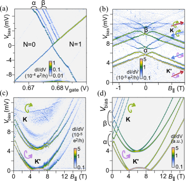
Figure 2: (a) Zero magnetic field differential conductance $\text{d}I/\text{d}V_{\text{bias}}$ of a CNT quantum dot with $0\leq N\leq 1$ conduction band electrons. Two pairs $\alpha$ and $\beta$ of conductance lines, all four representing Kramers doublets, are visible. (b) $\text{d}I/\text{d}V_{\text{bias}}$ for constant $V_{\text{gate}}=0.675\,\text{V}$ and varying $|B_{\parallel}|\leq 1.5\,\text{T}$. The Kramers doublets split at finite field into four states for both $\alpha$ and $\beta$. Spin and valley of the $\alpha$ states for $B_{\parallel}\gg 0.5\,\text{T}$ are indicated. (c) Differential conductance at the same $V_{\text{gate}}$, now for $B_{\parallel}$ up to $17\,\text{T}$. The four visible lines correspond to $K^{\prime}$ states in $\alpha$ and $\beta$; the $K$ lines fade out fast. (d) Calculated conductance, using the reduced density matrix technique and assuming field-independent tunneling coupling of all states to the leads. In contrast to the measurement, both $K$ and $K^{\prime}$ valley lines clearly persist at high magnetic field.

Figure 2(a) shows the stability diagram of the CNT in this gate voltage region. The resonance lines correspond to the single particle energies of the lowest discrete states of the quantum dot Laird et al. (2015). Two closely spaced sets $\alpha$ and $\beta$ of two Kramers doublets are visible. By fixing $V_{\text{gate}}$ and sweeping a magnetic field, the evolution of the states in the field can be recorded, see Figs. 2(b,c). The Kramers degeneracy is then lifted, revealing four states in each set.

Low field spectra similar to Fig. 2(b) have been reported by several groups Minot et al. (2004); Kuemmeth et al. (2008); Jespersen et al. (2011a); Steele et al. (2013) and are now well understood. A quantitative fit can be obtained by a model Hamiltonian for a single longitudinal mode, including valley mixing due to disorder or backscattering at the contact (see Jespersen et al. (2011a) and Sec. VI of the Supplement). For $\left|B_{\parallel}\right|>0.5\,\text{T}$, valley mixing is not relevant and the evolution of the spectral lines can be deduced from the Dirac equation, Eq. (2) below (see Sec. III of the Supplement for needed modifications). Valley and spin can be assigned to each excitation at higher fields, see Fig. 2(b).

We have traced the single particle states from Fig. 2(b) up to a high magnetic field of $B_{\parallel}=17\,\text{T}$. As visible in Figs. 2(b) and 2(c), the four $K$ lines evolve upwards in energy. They are comparatively weak, fading out already below $1\,\text{T}$. In contrast, the four $K^{\prime}$ conductance lines evolve initially downwards, gaining in strength, but then turn upwards above $6\,\text{T}$ and fade too. The presence of both weak $K$ and strong $K^{\prime}$ transitions in Fig. 2(c) at the same bias excludes the possibility of a trivial dependence of tunneling rates on the bias voltage. The model calculation of the conductance in Fig. 2(d), assuming a field independent $k_{\parallel}$, successfully follows the peak positions but clearly fails to reproduce the intensity variations, especially the suppression of $K$ lines already at low fields.

We show in the following that this effect results from the $B_{\parallel}$ dependence of the wave functions’ longitudinal profile. When the field is applied perpendicular to the CNT axis no such effect occurs and all excitation lines are present at almost constant strength; see Fig. S-10 in the Supplement, where this is experimentally reproduced over a wide gate voltage and electron number range sup .

Boundary conditions on bipartite lattices— The spatial profile of the wave functions $\psi(\bm{r})$ of a finite quantum system is determined by the boundary conditions and the resulting quantization of the wave vector. In unipartite lattices, e.g., monoatomic chains, hard-wall boundary conditions are $\psi(\bm{R}_{L})=0=\psi(\bm{R}_{R})$, where $\bm{R}_{L/R}$ are the lattice vectors of the first site beyond the left and right end of the chain, respectively. The linear combinations of Bloch states satisfying these conditions create standing waves with nodes at $\bm{R}_{L}$ and $\bm{R}_{R}$, as those of a half-wave resonator. Their wave vectors are quantized according to the familiar condition $k_{\parallel}=n\pi/L$, where $L$ is the length of the chain and $n\in\mathbb{N}$.

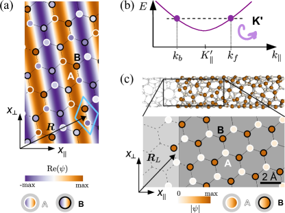
Figure 3: (a) Bloch function $\psi_{\bm{k}_{\!f}}$ in a (6,3) infinite CNT calculated at the atomic positions (filling of white-rimmed circles for the A sublattice, black-rimmed for B). The background shows a forward-propagating [$f$] plane wave with momentum $\bm{k}_{\!f}$. (b) Level diagram corresponding to forward [$f$] and backward [$b$] propagating states in the K’ valley. Standing waves in a finite CNT are composed of such states from the opposite sides of a Dirac cone at the same energy. (c) Left end of a (6,3) chiral CNT. The solid-drawn atoms and bonds belong to the quantum dot, the faint ones to the tunneling region. The calculated amplitude of the energy eigenstate formed by the superposition of $\psi_{\bm{k}_{\!f}}$ and $\psi_{\bm{k}_{b}}$ (circle filling / atom coloring) approaches zero towards the left end on the A atoms only.

The situation is more complex in bipartite lattices, as in the CNT shown in Fig. 3. The eigenstates are spinors in sublattice space, $\Psi^{\dagger}=(\psi_{A}^{\dagger},\psi_{B}^{\dagger})$, and near the Dirac points obey the Dirac equation

$$\hbar v_{F}\!\begin{pmatrix}0\quad\quad e^{i\tau\theta}(\tau\kappa_{\perp}-i\kappa_{\parallel})\\[5.69054pt] e^{-i\tau\theta}(\tau\kappa_{\perp}+i\kappa_{\parallel})\quad\quad 0\end{pmatrix}\!\!\!\begin{pmatrix}\psi_{\bm{k}A}\\ \psi_{\bm{k}B}\end{pmatrix}=E\!\begin{pmatrix}\psi_{\bm{k}A}\\ \psi_{\bm{k}B}\end{pmatrix}\!,$$ (2)

where $v_{F}$ is the Fermi velocity and $\theta$ is the CNT chiral angle. They have the form $\Psi_{\bm{k}}=w(e^{i\eta(\bm{k})}\psi_{\bm{k}A}+e^{-i\eta(\bm{k})}\psi_{\bm{k}B})$, with $w$ a normalization factor, meaning that there is a phase shift $2\eta(\bm{k})=-\tau\arctan(\kappa_{\parallel}/\kappa_{\perp})+\tau\theta$ between the two sublattice wavefunctions $\psi_{\bm{k}A}$ and $\psi_{\bm{k}B}$. On the $A$ atoms the phase is advanced by $\eta(\bm{k})$ with respect to the plane wave part of the Bloch state, on the $B$ atoms it is retarded. This is illustrated in Fig. 3(a), where the real part of the plane wave $e^{i\bm{k}_{\!f}\cdot\bm{r}}$ is plotted in the background, and the real part of the complete Bloch function $\Psi_{\bm{k}_{\!f}}(\bm{r})$ at each atomic position is shown as the filling of the white (sublattice $A$) and black (sublattice $B$) circles.

Standing waves in a finite CNT are formed by appropriate linear combinations of forward [$f$] and backward [$b$] propagating waves of the same energy, see Fig. 3(b). A specific combination of Bloch states $\Psi=c_{f}\Psi_{\bm{k}_{f}}+c_{b}\Psi_{\bm{k}_{b}}$ may satisfy the boundary condition $\psi_{A}(\bm{R}_{L})=0$, but then in general $\psi_{B}(\bm{R}_{L})\neq 0$. The counterpropagating Bloch waves interfering destructively on $A$ remain finite on $B$ because they are superposed with different phases, see Fig. 3(c). There is no non-trivial superposition with nodes at both ends for both sublattice components. Thus, the boundary conditions for bipartite lattices are either $\psi_{A}(\bm{R}_{L})=0=\psi_{B}(\bm{R}_{R})$ or $\psi_{A}(\bm{R}_{R})=0=\psi_{B}(\bm{R}_{L})$, depending on the sublattice to which the majority of the relevant edge atoms belongs Akhmerov and Beenakker (2008); Marganska et al. (2011); not .

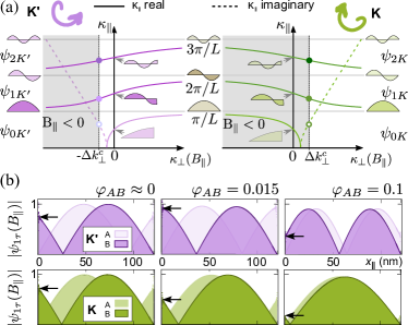
Figure 4: (a) The first solutions of Eq. (3) in the $K^{\prime}$ and $K$ valley for a chiral CNT. The wave function envelope is sketched for $\kappa_{\perp}=0$ and large $\kappa_{\perp}$. Dots mark the values of $\kappa_{\parallel}$ at $B_{\parallel}=0$. (b) Calculated amplitude of the longitudinal wave functions $\psi_{1\tau}(x_{\parallel},B_{\parallel})$ of the $K^{\prime}$ (top row) and $K$ (bottom row) valley states for a (15,3) chiral CNT with $L=121\,\text{nm}$. Black arrows mark $|\psi_{1\tau}|$ on the $B$ sublattice at the left end.

The superposition of forward and backward moving Bloch states with $\pm\kappa_{\parallel}$ and the same $\tau\kappa_{\perp}$, together with the bipartite boundary conditions, leads to the unusual quantization condition Akhmerov and Beenakker (2008); Castro Neto et al. (2009); Marganska et al. (2011)

$$e^{2i\kappa_{\parallel}L}\overset{!}{=}e^{-2i\eta(\bm{k})}\,e^{i\tau\theta}=\frac{\tau\kappa_{\perp}+i\kappa_{\parallel}}{\tau\kappa_{\perp}-i\kappa_{\parallel}}.$$ (3)

Since Eq. (3) couples the transverse and the longitudinal direction, it can be seen as a cross-quantization condition. It implies that in an axial field also $k_{\parallel}$ depends on $B_{\parallel}$.

The solutions of Eq. (3) are plotted as coloured lines in Fig. 4(a). For comparison, the grey lines parallel to the $k_{\perp}$ axis correspond to the familiar half-wave solutions. The envelope wave function on the $A$ sublattice is also sketched; the $B$ counterpart is its mirror image. When $k_{\parallel}$ is close to a multiple of $\pi/L$ (for large $B_{\parallel}$), the wave function has the standard half-wave shape with a node at each end. At low field, the profile on each sublattice is close to a quarter-wave, with an antinode at the corresponding unconstrained end.

Figure 4(b) shows the calculated wave function amplitudes for the lowest mode ($n=1$), $|\psi_{1\tau}(x_{\parallel})|$ on the $A$ and $B$ sublattices, of a (15,3) CNT with $L=121\,\text{nm}$. They were obtained by direct diagonalization of a tight-binding Hamiltonian on finite lattice, with four valence orbitals per atom (for clarity without spin dependence) Izumida et al. (2009); Klinovaja et al. (2011). The shapes follow closely the expectations based on our analysis of Eq. (3).

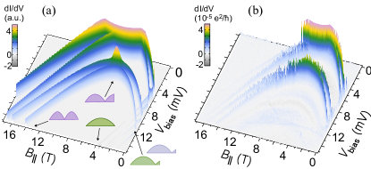
Figure 5: (a) Differential conductance calculated using the cross-quantization condition, Eq. (3), and thus field-dependent tunneling couplings. The wave functions $\psi_{K}(x_{\parallel},B_{\parallel})$ and $\psi_{K^{\prime}}(x_{\parallel},B_{\parallel})$ are assumed to represent the mode $n=1$, with parameters identical for both sets $\alpha$ and $\beta$ (cf. Fig. 2) and spin independent. (b) 3-dimensional plot of the data of Fig. 2(c), showing clearly the variation of peak heights with $B_{\parallel}$.

Fading of the differential conductance— To explain the fading conductance lines in Figs. 2(b,c), we account for the $B_{\parallel}$-dependence of the longitudinal CNT wave function in our transport calculations. This implies a $B_{\parallel}$ dependent tunneling amplitude, given by the overlap between CNT and lead wave functions in the contact region. In the single electron regime of the experiment, tunneling is weak and the tunneling amplitude is to a good approximation determined by the value of the CNT wavefunction at the quantum dot ends. The tunnel coupling at the left ($L$) contact is then

$$\Gamma_{L\mu}(B_{\parallel})=\alpha_{L}\frac{2\pi}{\hbar}|\psi_{B\mu}(x_{\parallel}=0,B_{\parallel})|^{2},$$ (4)

where $\mu=(n,\tau,\sigma)$ is a collective index accounting for the mode, valley, and spin, and $\alpha_{L}$ contains both the square modulus of the lead wave function at the contact and the lead density of states. The tunnel coupling at the right ($R$) contact is obtained by replacing $A\leftrightarrow B$ and $L\leftrightarrow R$. The factors $\alpha_{l}$ ($l=L,R$) encode a possible contact asymmetry. The differential conductance then follows from a reduced density matrix approach to lowest order in $\Gamma_{l\mu}$ Koller et al. (2010); sup . A calculation assuming $\alpha_{L}/\alpha_{R}=1/4$ is shown in Fig. 5(a). The input parameters for Eqs. (1) and (3) (nanotube radius, length, and $\Delta k_{\perp}^{c}$) were obtained by fitting the measured position of the spectral lines shown in Fig. 2(b,c) to the spectrum of the CNT model Hamiltonian, see Sec. III of the Supplement. The fast disappearance of the $K$ lines is in excellent agreement with the data plotted in Fig. 5(b). The suppression of $K^{\prime}$ lines at high field is also clearly reproduced.

In our calculations hard wall boundary conditions were assumed. In the experiment, though, we expect smooth confinement due to electrostatic gating, cf. Fig. S-6 of the Supplement. Hence, we have performed numerical calculations of the CNT eigenmodes as a function of $B_{\parallel}$ for a soft confinement, see Sec. V of the Supplement sup . We find qualitative agreement with the hard wall confinement calculation. Thus, the tunability of the longitudinal wave function with magnetic field occurs for smooth confinement as well.

In conclusion, our experiment can be regarded as the complement of a scanning tunneling microscopy (STM) measurement. In STM the spatial profile of atomic or molecular orbitals is obtained by scanning the tip position over the sample. In CNT quantum dots, the contact position is fixed, but the wavefunction, and thus the tunnel current, is tuned by an axial magnetic field. We are aware of only one other system in which such coupling has been found, a semiconducting quantum dot with pyramid shape Cao et al. (2015). The unusual tunability of the wave function shape with a parallel magnetic field will influence all phenomena dependent on the full spatial profile of the electronic states, such as, e.g., electron-phonon coupling or electron-electron interaction. Thus the parallel magnetic field is an even more versatile tool to investigate and control complex quantum systems than already acknowledged.