Thermodynamics and criticality of supersymmetric spin chains with long-range interactions

Abstract

We study the thermodynamics and critical behavior of $\mathrm{su}(m|n)$ supersymmetric spin chains of Haldane–Shastry type with a chemical potential term. We obtain a closed-form expression for the partition function and deduce a description of the spectrum in terms of the supersymmetric version of Haldane’s motifs, which we apply to obtain an analytic expression for the free energy per site in the thermodynamic limit. By studying the low-temperature behavior of the free energy, we characterize the critical behavior of the chains with $1\leqslant m,n\leqslant 2$, determining the critical regions and the corresponding central charge. We also show that in the $\mathrm{su}(2|1)$, $\mathrm{su}(1|2)$ and $\mathrm{su}(2|2)$ chains the bosonic or fermionic densities can undergo first-order (discontinuous) phase transitions at $T=0$, in contrast with the previously studied $\mathrm{su}(2)$ case.

Keywords: integrable spin chains and vertex models, solvable lattice models, quantum criticality, quantum phase transitions

1 Introduction

Spin chains of Haldane–Shastry type have been extensively studied as the prototypical examples of one-dimensional lattice models with long-range interactions, due to their remarkable physical and mathematical properties. The best known of these models is the original Haldane–Shastry (HS) chain [1, 2], which consists of a circular array of $N$ equispaced spins with inverse-square two-body interactions. This chain is integrable [3, 4] and invariant under the quantum Yangian for arbitrary values of $N$, which in turn makes it possible to derive a complete description of its spectrum in terms of Haldane’s motifs [5]. From a more applied standpoint, the HS chain has appeared in such disparate contexts as conformal field theory [6, 7, 8], fractional statistics and anyons [6, 5, 9, 10], quantum chaos vs. integrability [11, 12, 13, 14, 15], quantum information theory [16] or quantum simulation of long-range magnetism [17]. One of the characteristic features of the HS chain is its close connection with the (dynamical) spin Sutherland model [18], whose spin degrees of freedom are governed by the HS Hamiltonian in the large coupling constant limit. Using this idea, known in the literature as Polychronakos’s freezing trick [19], it is possible to compute in closed form the chain’s partition function [11]. In fact, the same approach can be applied to the long-range dynamical spin models of Calogero [20] and Inozemtsev [21], which yield the so-called Polychronakos–Frahm (PF) [22, 23] and Frahm–Inozemtsev (FI) [24] spin chains. Although they are not translationally invariant, these chains share many fundamental properties with the original HS chain. For this reason, we shall collectively refer in this work to the HS, PF and FI chains as spin chains of Haldane–Shastry type.

In all the chains of HS type discussed in the previous paragraph, the term “spin” actually stands for $\mathrm{su}(m)$ spin. In fact, Haldane himself was the first to consider an $\mathrm{su}(m|n)$ supersymmetric version of the HS chain, whose sites can be occupied either by an $\mathrm{su}(m)$ boson or by an $\mathrm{su}(n)$ fermion [25]. An analogous supersymmetric chain of PF type was introduced shortly afterwards [26]. The partition function of both the HS and the PF supersymmetric chains have been exactly computed using the freezing trick [26, 27, 28], and their spectra have been fully described in terms of a suitable generalization of Haldane’s motifs [29, 30, 31]. On the other hand, the supersymmetric version of the Frahm–Inozemtsev chain [31] has received comparatively less attention in the literature. It should also be noted that, apart from their intrinsic interest, the supersymmetric chains of HS type are closely related to important models in condensed matter theory describing the dynamics of holes in a spin background. Indeed, the HS $\mathrm{su}(1|n)$ chain with $n>1$ is equivalent to the long-range $\mathrm{su}(n)$ $t$-$J$ model with equal exchange and transfer energies proportional to $(z_{i}-z_{j})^{-2}$, originally introduced by Kuramoto and Yokoyama [32].

The study of the thermodynamics of spin chains of HS type, which goes back to the early work of Haldane [6], has received a good deal of attention. In the latter reference the spinon description of the spectrum is used to deduce an expression for the entropy of the $\mathrm{su}(2)$ HS chain in the thermodynamic limit. A heuristic formula for the free energy of the PF chain appeared shortly afterwards in Ref. [23]. A similar result for the FI chain using the transfer matrix method was derived by Frahm and Inozemtsev [24], who also computed the magnetization of this chain in an external constant magnetic field. More recently, a comprehensive study of the thermodynamics of the three (spin $1/2$) chains of HS type in a constant magnetic field was performed in Ref. [33], using again the transfer matrix method. In the supersymmetric case, the thermodynamic functions of the $\mathrm{su}(1|1)$ HS chain (with a chemical potential term) have been exactly computed taking advantage of the equivalence of this model to a free, translationally invariant fermion system [34]. This approach cannot be applied to the $\mathrm{su}(1|1)$ PF and FI chains, since these models are not translationally invariant, nor in fact to any chain of HS type with $m$ or $n$ different from $1$. To the best of our knowledge, the thermodynamics of the supersymmetric chains of the latter type, or the non-supersymmetric ones with $m>2$, have not been analyzed in the literature.

The connection between the original $\mathrm{su}(2)$ HS chain and the level-$1$ $\mathrm{su}(2)$ Wess–Zumino–Novikov–Witten conformal field theory (CFT), stemming from the Yangian symmetry of both types of models, was already numerically observed by Haldane [1] and subsequently established by several authors in the (purely fermionic) $\mathrm{su}(n)$ case [6, 5, 35, 36]. Thus the $\mathrm{su}(n)$ HS chain (with no magnetic field or chemical potential term) is critical (gapless), with central charge $c=n-1$. This result was later extended to the $\mathrm{su}(m|n)$ PF chain (again with zero chemical potentials) in Ref. [29], where it was shown that the central charge in this case is $c=m-1+n/2$ for $m\geqslant 1$. The same is true for the $\mathrm{su}(m|n)$ HS chain with $m\geqslant 1$, by virtue of the relation between the partition functions of the supersymmetric PF and HS chains established in Ref. [7]. The criticality of the $\mathrm{su}(1|1)$ HS chain with a chemical potential was also proved in Ref. [34], where it was shown that the central charge is instead $c=1$ for a certain range of nonzero values of the chemical potential. In particular, it should be noted that in all cases reviewed above the central charge is integer or half-integer, as in a CFT of free bosons and/or fermions.

The aim of this paper is to study the thermodynamics and the critical behavior of the three families of $\mathrm{su}(m|n)$ spin chains of HS type with a general chemical potential term. To this end, we shall first evaluate in closed form the chains’ partition functions for arbitrary finite values of the number of sites $N$. Exploiting the connection of the latter chains with a certain inhomogeneous vertex model, we shall achieve a concise description of the spectrum in terms of a generalization of Haldane’s motifs. This description shall then be used to compute the transfer matrix and obtain a closed-form expression for the free energy per site in the thermodynamic limit. With the help of this expression, we shall study the thermodynamics and criticality of the supersymmetric chains of HS type with $1\leqslant m,n\leqslant 2$. First of all, examining the low-temperature behavior of the free energy per site we shall determine the values of the chemical potentials for which these chains are critical, and compute the corresponding central charge. In particular, it turns out that the central charge can take rational values that are not half-integers. We shall also analyze the existence of phase transitions at zero temperature in the densities of bosons and fermions. We shall show that these densities exhibit only second-order (continuous) transitions for $m=n=1$, while for $m+n>2$ (and $1\leqslant m,n\leqslant 2$) either the bosonic or the fermionic densities undergo a first-order (discontinuous) phase transition.

We shall end this introduction by briefly outlining the paper’s organization. In Section 2 we present the three supersymmetric chains of HS type under study, and discuss their duality under exchange of the bosonic and fermionic degrees of freedom. The partition function of these chains is computed in closed form in Section 3 by means of Polychronakos’s freezing trick. In Section 4 we establish the equivalence of $\mathrm{su}(m|n)$ supersymmetric spin chains of HS type to certain inhomogeneous vertex models, from which we deduce a simple formula for the spectrum in terms of supersymmetric motifs. By means of this formula, in Section 5 we evaluate the chains’ free energy per site in the thermodynamic limit. We also discuss in this section several symmetries of the free energy and the main thermodynamic functions, with particular emphasis on the one arising from the boson-fermion duality. Sections 6-8 are devoted to the analysis of the critical behavior and the existence of zero-temperature phase transitions in the spin densities for the $\mathrm{su}(1|1)$, $\mathrm{su}(2|1)$ and $\mathrm{su}(2|2)$ chains. In Section 9 we present our conclusions and discuss several lines for future research suggested by the present work. The paper ends with a technical appendix providing a detailed discussion of the behavior of the free energy per site of the $\mathrm{su}(1|1)$ chains for finite values of $N$.

2 The models

An $\mathrm{su}(m|n)$ supersymmetric spin chain is a one-dimensional array of $N$ sites, each of which is occupied by either a boson or a fermion with $m$ and $n$ degrees of freedom, respectively. Thus the Hilbert space $\Sigma^{(m|n)}=\otimes_{i=1}^{N}{\mathbb{C}}^{m+n}$ of the system is spanned by the basis vectors

$$|s_{1}\cdots s_{N}\rangle\equiv|s_{1}\rangle\otimes\cdots\otimes|s_{N}\rangle,\qquad s_{i}\in\{1,\dots,m+n\},$$ (2.1)

where the one-particle state $|s_{i}\rangle$ is regarded as bosonic if $s_{i}\in B\equiv\{1,\dots,m\}$ and fermionic if $s_{i}\in F\equiv\{m+1,\dots,m+n\}$. The $\mathrm{su}(m|n)$ permutation operators $P_{ij}^{(m|n)}$ (with $1\leqslant i<j\leqslant N$) are defined by

$$P_{ij}^{(m|n)}|\cdots s_{i}\cdots s_{j}\cdots\rangle=\epsilon_{ij}(s_{1},\dots,s_{N})|\cdots s_{j}\cdots s_{i}\cdots\rangle,$$ (2.2)

where the sign $\epsilon_{ij}(s_{1},\dots,s_{N})$ is equal to $1$ if $s_{i},s_{j}\in B$, $-1$ if $s_{i},s_{j}\in F$, and $(-1)^{\nu}$ if $s_{i}$ and $s_{j}$ are of different type, $\nu$ being the number of fermionic spins $s_{k}$ with $k=i+1,\dots,j-1$. We shall also define the number operators ${\mathcal{N}}_{\alpha}$ with $\alpha=1,\dots,m+n$ by

$${\mathcal{N}}_{\alpha}|s_{1}\cdots s_{N}\rangle=N_{\alpha}(\mathbf{s})|s_{1}\cdots s_{N}\rangle,$$

where

$$N_{\alpha}(\mathbf{s})\equiv\sum_{i=1}^{N}\delta_{s_{i},\alpha}$$ (2.3)

is the number of spins of type $\alpha$ in the state $|s_{1}\cdots s_{N}\rangle$. The supersymmetric spin chains we shall deal with in this paper are described by a Hamiltonian of the form

$${\mathcal{H}}=\sum_{i<j}J_{ij}(1-P_{ij}^{(m|n)})-\sum_{\alpha=1}^{m+n-1}\mu_{\alpha}{\mathcal{N}}_{\alpha}\equiv{\mathcal{H}}_{0}+{\mathcal{H}}_{1},$$ (2.4)

where (as in what follows, unless otherwise stated) the sum over Latin indices ranges from $1$ to $N$. In the last term the real constant $\mu_{\alpha}$ has a natural interpretation as the chemical potential of the $\alpha$-th species, and without loss of generality (since $\sum_{\alpha=1}^{m+n}{\mathcal{N}}_{\alpha}=N$) we have chosen the normalization $\mu_{m+n}=0$. The models we shall focus on are those for which ${\mathcal{H}}_{0}$ is the Hamiltonian of the supersymmetric Haldane–Shastry, Polychronakos–Frahm and Frahm–Inozemtsev spin chains, whose interaction strengths $J_{ij}$ are respectively given by

$$J_{ij} =\frac{J}{2\sin^{2}(\xi_{i}-\xi_{j})},\qquad \xi_{k}=\frac{k\pi}{N}\,,$$ (2.5)

$$J_{ij} =\frac{J}{(\xi_{i}-\xi_{j})^{2}}\,,\qquad H_{N}(\xi_{k})=0\,,$$ (2.6)

$$J_{ij} =\frac{J}{2\sinh^{2}(\xi_{i}-\xi_{j})}\,,\qquad L_{N}^{c-1}(\rme^{2\xi_{k}})=0\,.$$ (2.7)

Here $J\neq 0$ is a real constant, $H_{N}$ denotes the Hermite polynomial of degree $N$ and $L_{N}^{c-1}$ is a generalized Laguerre polynomial of degree $N$ (with $c$ a positive parameter).

In the non-supersymmetric case ($mn=0$) the model (2.4) with interactions (2.5)–(2.7) is the one solved in Ref. [33]. Indeed, in this case $P_{ij}=\pm S_{ij}$, where $S_{ij}$ is the operator permuting the $i$-th and $j$-th spins and the “$+$” (resp. “$-$”) sign corresponds to the case $n=0$ (resp. $m=0$). Moreover, the operators

$${\mathcal{J}}_{\alpha}={\mathcal{N}}_{\alpha}-{\mathcal{N}}_{m+n}\,,\qquad\alpha=1,\dots,m+n-1\,,$$

are a basis of the standard $\mathrm{su}(m+n)$ Cartan subalgebra, in terms of which ${\mathcal{H}}_{1}$ can be expressed as

$${\mathcal{H}}_{1}=\sum_{\alpha=1}^{m+n-1}B_{\alpha}{\mathcal{J}}_{\alpha}+B_{0}$$

for suitable real constants $B_{\alpha}$. It also worth mentioning that the Hamiltonian (2.4), for which we shall use the more explicit notation ${\mathcal{H}}^{(m|n)}$, is related to ${\mathcal{H}}^{(n|m)}$ by a duality relation that we shall now briefly explain [30, 37]. To this end, let us define the unitary operator $U:\Sigma^{(m|n)}\to\Sigma^{(n|m)}$ by

$$U|s_{1}\cdots s_{N}\rangle=(-1)^{\sum_{i}i\pi(s_{i})}|s_{1}^{\prime}\cdots s_{N}^{\prime}\rangle\,,$$

where $\pi(s_{i})=0$ if $s_{i}\in B$ (resp. $\pi(s_{i})=1$ if $s_{i}\in F$) and $s_{i}^{\prime}=m+n+1-s_{i}$. We then have

$$U^{-1}P_{ij}^{(n|m)}U=-P_{ij}^{(m|n)}\,,\qquad U^{-1}{\mathcal{N}}_{\alpha}U={\mathcal{N}}_{m+n+1-\alpha}\,,$$

and therefore

$$U^{-1}{\mathcal{H}}^{(n|m)}U=E_{0}-{\mathcal{H}}^{(m|n)}\Big{|}_{\mu_{\alpha}\to-\mu_{m+n+1-\alpha}},\qquad E_{0}\equiv 2\sum_{i<j}J_{ij}\,.$$ (2.8)

Thus the spectra of ${\mathcal{H}}^{(n|m)}$ and ${\mathcal{H}}^{(m|n)}$ are related by

$$E_{k}^{(n|m)}(\mu_{1},\dots,\mu_{m+n})=E_{0}-E_{k}^{(m|n)}(-\mu_{m+n},\dots,-\mu_{1})\,.$$ (2.9)

We can therefore assume without loss of generality that $m\geqslant n$ in what follows.

Another basic symmetry of the spectrum of the Hamiltonian (2.4) is related to changes in the labeling of the bosonic or fermionic degrees of freedom. More precisely, let $T_{\alpha\beta}:\Sigma^{(m|n)}\to\Sigma^{(m|n)}$ (with $\alpha\neq\beta\in\{1,\dots,m+n\}$) denote the linear operator whose action on a basis element $|s_{1}\cdots s_{N}\rangle$ consists in replacing all the $s_{k}$’s equal to $\alpha$ by $\beta$, and vice versa. If $\pi(\alpha)=\pi(\beta)$ (i.e., if $\alpha$ and $\beta$ are either both bosonic or both fermionic) it is clear that $T_{\alpha\beta}$ commutes with the $\mathrm{su}(m|n)$ permutation operators $P_{ij}^{(m|n)}$, and hence with ${\mathcal{H}}_{0}$. It is also straightforward to verify that

$$T_{\alpha\beta}^{-1}\,{\mathcal{N}}_{\alpha}\,T_{\alpha\beta}={\mathcal{N}}_{\beta}\,,\qquad T_{\alpha\beta}^{-1}\,{\mathcal{N}}_{\beta}\,T_{\alpha\beta}={\mathcal{N}}_{\alpha}\,,\qquad T_{\alpha\beta}^{-1}\,{\mathcal{N}}_{\gamma}\,T_{\alpha\beta}={\mathcal{N}}_{\gamma}\quad(\gamma\neq\alpha,\beta),$$

and thus

$$T_{\alpha\beta}^{-1}\,{\mathcal{H}}\,T_{\alpha\beta}={\mathcal{H}}_{0}-\mu_{\alpha}{\mathcal{N}}_{\beta}-\mu_{\beta}{\mathcal{N}}_{\alpha}-\sum_{\substack{\gamma=1\cr\gamma\neq\alpha,\beta}}^{m+n}\mu_{\gamma}{\mathcal{N}}_{\gamma}\,.$$

It follows that

$$E_{k}^{(m|n)}(\dots,\mu_{\alpha},\dots,\mu_{\beta},\dots)=E_{k}^{(m|n)}(\dots,\mu_{\beta},\dots,\mu_{\alpha},\dots)\qquad(\pi(\alpha)=\pi(\beta));$$ (2.10)

in other words, the spectrum of ${\mathcal{H}}$ is invariant under permutations of the bosonic or fermionic chemical potentials among themselves. Note, finally, that combining Eqs. (2.9) and (2.10) we obtain the more general relation

$$E_{k}^{(n|m)}(\mu_{1},\dots,\mu_{m+n})=E_{0}-E_{k}^{(m|n)}(-\mu_{\alpha_{1}},\dots,-\mu_{\alpha_{m+n}})\,,$$

where $(\alpha_{1},\dots,\alpha_{m+n})$ is a permutation of $(1,\dots,m+n)$ such that $\{\alpha_{1},\dots,\alpha_{m}\}=\{n+1,\dots,n+m\}$ (and, consequently, $\{\alpha_{m+1},\dots,\alpha_{m+n}\}=\{1,\dots,n\})$.

3 Partition function

In this section we shall compute in closed form the partition function of the chains (2.4)–(2.7) by exploiting their connection with the $\mathrm{su}(m|n)$ spin versions [25, 38, 27, 26] of the dynamical models of Sutherland, Calogero and Inozemtsev, respectively. For definiteness, we shall present the details of the calculation only for the PF model (2.4)-(2.6), which is technically the simplest.

To begin with, recall that the Hamiltonian of the $\mathrm{su}(m|n)$ spin Calogero model is given by

$$H_{0}=-\sum_{i}\partial_{x_{i}}^{2}+a^{2}r^{2}+\sum_{i\neq j}\frac{a\big{(}a-{P}^{(m|n)}_{ij}\big{)}}{(x_{i}-x_{j})^{2}},\qquad r^{2}\equiv\sum_{i}x_{i}^{2}\,,$$ (3.1)

with scalar counterpart

$$H_{\mathrm{sc}}=-\sum_{i}\partial_{x_{i}}^{2}+a^{2}r^{2}+\sum_{i\neq j}\frac{a(a-1)}{(x_{i}-x_{j})^{2}}.$$ (3.2)

Defining

$$H=H_{0}+\frac{2a}{J}\,{\mathcal{H}}_{1}$$ (3.3)

we then have

$$H=H_{\mathrm{sc}}+\frac{2a}{J}\,h(\mathbf{x})\,,$$ (3.4)

with $\mathbf{x}\equiv(x_{1},\dots,x_{N})$ and

$$h(\mathbf{x})=J\sum_{i<j}\frac{1-P_{ij}^{(m|n)}}{(x_{i}-x_{j})^{2}}-\sum_{\alpha=1}^{m+n-1}\mu_{\alpha}{\mathcal{N}}_{\alpha}\,.$$

Hence the Hamiltonian (2.4) with interactions (2.6) is simply ${\mathcal{H}}=h(\boldsymbol{\xi})$, where $\boldsymbol{\xi}\equiv(\xi_{1},\dots,\xi_{N})$ and the $\xi_{k}$’s are the chain sites (i.e., the zeros of the Hermite polynomial of degree $N$). From Eq. (3.1) it follows that in the limit $a\to\infty$ the eigenfunctions of the $\mathrm{su}(m|n)$ spin Hamiltonian $H$ are sharply peaked at the coordinates of the (unique) equilibrium of the scalar potential

$$U=r^{2}+\sum_{i\neq j}\frac{1}{(x_{i}-x_{j})^{2}}$$ (3.5)

in the configuration space ($A_{N-1}$ Weyl chamber)

$$A=\{\mathbf{x}\in{\mathbb{R}}^{N}|x_{1}<\cdots<x_{N}\}\,,$$

which coincide with the chain sites $\xi_{k}$ [39]. By Eq. (3.4) and the relation ${\mathcal{H}}=h(\boldsymbol{\xi})$, it follows that for large $a$ the eigenvalues of $H$ are approximately given by

$$E_{ij}\simeq E^{\mathrm{sc}}_{i}+\frac{2a}{J}\,e_{j}\,,$$

where $E^{\mathrm{sc}}_{i}$ and $e_{j}$ respectively denote two arbitrary eigenvalues of $H_{\mathrm{sc}}$ and ${\mathcal{H}}$. From the latter equation it is immediate to deduce the following exact formula relating the partition functions $Z$, $Z_{\mathrm{sc}}$ and $\mathcal{Z}$ of the three Hamiltonians $H$, $H_{\mathrm{sc}}$ and ${\mathcal{H}}$:

$$\mathcal{Z}(T)=\lim_{a\to\infty}\frac{Z(2aT/J)}{Z_{\mathrm{sc}}(2aT/J)}.$$ (3.6)

The argument just outlined leading to Eq. (3.6) is known in the literature as Polychronakos’s freezing trick [19].

The partition function $Z_{\mathrm{sc}}$ of the scalar Calogero model (3.2), which is well known (see, e.g., Refs. [19, 12]), is given by

$$Z_{\mathrm{sc}}(2aT/J)=q^{\frac{JE_{\mathrm{GS}}}{2a}}\prod_{i}(1-q^{Ji})^{-1},\qquad q\equiv\rme^{-1/T},$$ (3.7)

where

$$E_{\mathrm{GS}}=aN+a^{2}N(N-1)$$

is the ground-state energy of both $H_{0}$ and $H_{\mathrm{sc}}$, and we have taken Boltzmann’s constant $k_{\mathrm{B}}$ as $1$. We shall next outline the computation of the spectrum of the Hamiltonian $H$ in Eq. (3.3). To this end, note first of all that, although the Hamiltonians $H_{0}$ and $H$ are naturally defined on the Hilbert space $L^{2}(A)\otimes\Sigma^{(m|n)}$, they are actually equivalent to any of their extensions to the space $L^{2}({\mathbb{R}}^{N})\otimes\Sigma^{(m|n)}$. This is essentially due to the fact that any point $\mathbf{x}\in{\mathbb{R}}^{N}$ outside the singular hyperplanes $x_{i}-x_{j}=0$ can be mapped in a unique way to a point in $A$ by an appropriate permutation. For reasons that will be clear in the sequel, from now on we shall identify $H_{0}$ and $H$ with their symmetric extension, defined on the Hilbert space $\Lambda(L^{2}({\mathbb{R}}^{N})\otimes\Sigma^{(m|n)})$. Here $\Lambda$ is the total symmetrizer with respect to simultaneous permutations of both the coordinates and the spin variables, determined by the relations

$$K_{ij}{P}^{(m|n)}_{ij}\Lambda=\Lambda K_{ij}{P}^{(m|n)}_{ij}=\Lambda,\qquad 1\leqslant i<j\leqslant N\,,$$ (3.8)

where $K_{ij}$ denotes the operator permuting the $i$-th and $j$-th coordinates. With the latter identification, it can be shown that $H$ is represented by an upper triangular matrix in an appropriate basis that we shall now describe. To this end, let

$$|\mathbf{n},\mathbf{s}\rangle=\Lambda\Big{(}\rho(\mathbf{x})\prod_{i}x_{i}^{n_{i}}\cdot|\mathbf{s}\rangle\Big{)},$$ (3.9)

where $|\mathbf{s}\rangle\equiv|s_{1}\cdots s_{N}\rangle$ and

$$\rho(\mathbf{x})=\rme^{-ar^{2}/2}\prod_{i<j}|x_{i}-x_{j}|^{a}.$$ (3.10)

The states (3.9), partially ordered according to the total degree $|\mathbf{n}|\equiv\sum_{i}n_{i}$, are a (non-orthonormal) basis of $\Lambda(L^{2}({\mathbb{R}}^{N})\otimes\Sigma^{(m|n)})$ provided that (for instance) the quantum numbers $\mathbf{n}$ and $\mathbf{s}$ satisfy the following conditions

1. $n_{i}\geqslant n_{i+1}$ for all $i=1,\dots,N-1$.

2. If $n_{i}=n_{i+1}$ then $s_{i}\leqslant s_{i+1}$ for $s_{i}\in B$, or $s_{i}<s_{i+1}$ for $s_{i}\in F$.

Indeed, note first of all that if $n_{i}=n_{j}$ and $s_{i}=s_{j}\in F$ then the state (3.9) vanishes by antisymmetry. Otherwise, acting with the permutation operators $K_{ij}P_{ij}$ on a state of the form (3.9) we can always obtain a state satisfying the first condition and differing from the original one at most by a sign. Applying to this state permutations acting on indices $i,j$ such that $n_{i}=n_{j}$ we arrive at a state, again differing from the initial one by at most a sign, in which the spin variables are ordered so that the second condition is also satisfied. Moreover, it can be shown that the states satisfying the above two conditions are linearly independent and complete.

Proceeding as in Ref. [12], it is straightforward to show that the action of the spin Hamiltonian $H_{0}$ on the basis (3.9) is given by

$$H_{0}|\mathbf{n},\mathbf{s}\rangle=E_{\mathbf{n},\mathbf{s}}^{0}|\mathbf{n},\mathbf{s}\rangle+\sum_{|\mathbf{n}^{\prime}|<|\mathbf{n}|,\mathbf{s}^{\prime}}c_{\mathbf{n}^{\prime}\mathbf{s}^{\prime},\mathbf{n}\mathbf{s}}|\mathbf{n}^{\prime},\mathbf{s}^{\prime}\rangle$$ (3.11)

with $c_{\mathbf{n}^{\prime}\mathbf{s}^{\prime},\mathbf{n}\mathbf{s}}\in{\mathbb{C}}$ and

$$E_{\mathbf{n},\mathbf{s}}^{0}=2a|\mathbf{n}|+E_{\mathrm{GS}}\,.$$ (3.12)

The matrix of $H_{0}$ on the basis (3.9) is upper triangular, as claimed, and its spectrum is given by Eq. (3.12). On the other hand, since ${\mathcal{H}}_{1}$ clearly commutes with the symmetrizer $\Lambda$ (since each ${\mathcal{N}}_{\alpha}$ does) and

$${\mathcal{H}}_{1}|\mathbf{s}\rangle=-\sum_{\alpha=1}^{m+n-1}\mu_{\alpha}N_{\alpha}(\mathbf{s})|\mathbf{s}\rangle=-\Big{(}\sum_{i}\mu_{s_{i}}\Big{)}|\mathbf{s}\rangle$$

(with $\mu_{m+n}=0$), we have

$${\mathcal{H}}_{1}|\mathbf{n},\mathbf{s}\rangle=-\Big{(}\sum_{i}\mu_{s_{i}}\Big{)}|\mathbf{n},\mathbf{s}\rangle\,.$$ (3.13)

Thus ${\mathcal{H}}_{1}$ is diagonal in the basis (3.9), and by Eqs. (3.11)-(3.13) the spectrum of $H$ is given by

$$E_{\mathbf{n},\mathbf{s}}=2a|\mathbf{n}|-\frac{2a}{J}\,\sum_{i}\mu_{s_{i}}+E_{\mathrm{GS}}\,,$$ (3.14)

where the quantum numbers $\mathbf{n}$ and $\mathbf{s}$ satisfy conditions i)-ii) above.

We are now ready to evaluate in closed form the partition function of the chain (2.4) using the freezing trick formula (3.6). In the first place, in order to compute the partition function of the $\mathrm{su}(m|n)$ spin model (3.3) it is convenient to parametrize the multiindex $\mathbf{n}$ satisfying condition i) above as

$$\mathbf{n}=(\underbrace{\nu_{1},\dots,\nu_{1}}_{k_{1}},\dots,\underbrace{\nu_{r},\dots,\nu_{r}}_{k_{r}}),$$ (3.15)

where $\nu_{1}>\cdots>\nu_{r}\geqslant 0$ and $k_{1}+\cdots+k_{r}=N$ with $k_{i}>0$ for all $i$. In particular, note that the vector $\mathbf{k}=(k_{1},\dots,k_{r})$ can be considered as an element of the set ${\mathcal{P}}_{N}$ of ordered partitions of the integer $N$. We shall also refer in what follows to each maximal group $(\nu_{i},\dots,\nu_{i})$ of repeated components of the multiindex $\mathbf{n}$ as a sector. From Eq. (3.14) for the spectrum of $H$ it immediately follows that the partition function $H$ is given by

$$Z(2aT/J)=q^{\frac{JE_{\mathrm{GS}}}{2a}}\sum_{\mathchoice{\hbox to0.0pt{\hss$\displaystyle{\mathbf{k}\in{\mathcal{P}}_{N}}$\hss}}{\hbox to0.0pt{\hss$\textstyle{\mathbf{k}\in{\mathcal{P}}_{N}}$\hss}}{\hbox to0.0pt{\hss$\scriptstyle{\mathbf{k}\in{\mathcal{P}}_{N}}$\hss}}{\hbox to0.0pt{\hss$\scriptscriptstyle{\mathbf{k}\in{\mathcal{P}}_{N}}$\hss}}}\qquad\sum_{\mathchoice{\hbox to0.0pt{\hss$\displaystyle{\nu_{1}>\cdots>\nu_{r}\geqslant 0}$\hss}}{\hbox to0.0pt{\hss$\textstyle{\nu_{1}>\cdots>\nu_{r}\geqslant 0}$\hss}}{\hbox to0.0pt{\hss$\scriptstyle{\nu_{1}>\cdots>\nu_{r}\geqslant 0}$\hss}}{\hbox to0.0pt{\hss$\scriptscriptstyle{\nu_{1}>\cdots>\nu_{r}\geqslant 0}$\hss}}}q^{\sum\limits_{i=1}^{r}Jk_{i}\nu_{i}}\sum_{\mathbf{\mathbf{s}}\in\mathbf{n}}q^{-\sum_{j}\mu_{s_{j}}},$$ (3.16)

where the notation $\mathbf{s}\in\mathbf{n}$ stands for all possible multiindices $\mathbf{s}\in\{1,\dots,m+n\}^{N}$ satisfying condition ii) above for a given multiindex $\mathbf{n}$. Let us next evaluate the inner sum in Eq. (3.16)

$$\Sigma(\mathbf{k})\equiv\sum_{\mathbf{\mathbf{s}}\in\mathbf{n}}q^{-\sum_{j}\mu_{s_{j}}},$$ (3.17)

which clearly depends on $\mathbf{n}$ only through $\mathbf{k}$. Since condition ii) above effects only the ordering of the spin variables $s_{k}$ within each sector of the multiindex $\mathbf{n}$ independently of the others, we have

$$\Sigma(\mathbf{k})\equiv\prod_{i=1}^{r}\sigma(k_{i})\,,$$ (3.18)

where

$$\sigma(k)=\sum_{i+j=k}\qquad\sum_{\mathchoice{\hbox to0.0pt{\hss$\displaystyle{1\leqslant s_{1}\leqslant\cdots\leqslant s_{i}\leqslant m}$\hss}}{\hbox to0.0pt{\hss$\textstyle{1\leqslant s_{1}\leqslant\cdots\leqslant s_{i}\leqslant m}$\hss}}{\hbox to0.0pt{\hss$\scriptstyle{1\leqslant s_{1}\leqslant\cdots\leqslant s_{i}\leqslant m}$\hss}}{\hbox to0.0pt{\hss$\scriptscriptstyle{1\leqslant s_{1}\leqslant\cdots\leqslant s_{i}\leqslant m}$\hss}}}q^{-\sum\limits_{l=1}^{i}\mu_{s_{l}}}\kern 7.5pt\sum_{\mathchoice{\hbox to0.0pt{\hss$\displaystyle{1\leqslant l_{1}<\cdots<l_{j}\leqslant n}$\hss}}{\hbox to0.0pt{\hss$\textstyle{1\leqslant l_{1}<\cdots<l_{j}\leqslant n}$\hss}}{\hbox to0.0pt{\hss$\scriptstyle{1\leqslant l_{1}<\cdots<l_{j}\leqslant n}$\hss}}{\hbox to0.0pt{\hss$\scriptscriptstyle{1\leqslant l_{1}<\cdots<l_{j}\leqslant n}$\hss}}}q^{-\sum\limits_{p=1}^{j}\mu_{m+l_{p}}}$$ (3.19)

is the contribution to $\Sigma(\mathbf{k})$ of a sector of length $k$ (with $i$ bosons and $j$ fermions). The sum $\sigma(k)$ is easily expressed in terms of the complete and elementary symmetric polynomials $h_{i}(x_{1},\dots,x_{m})$ and $e_{j}(x_{1},\dots,x_{n})$ of degrees $i$ and $j$, respectively defined by

$$h_{i}(x_{1},\dots,x_{m})\equiv\sum_{p_{1}+\cdots+p_{m}=i}x_{1}^{p_{1}}\cdots x_{m}^{p_{m}}\,,\qquad e_{j}(x_{1},\dots,x_{n})\equiv\sum_{1\leqslant l_{1}<\cdots<l_{j}\leqslant n}x_{l_{1}}\cdots x_{l_{j}}\,,$$

where it is understood that $e_{j}(x_{1},\dots,x_{n})=0$ for $j>n$. Recall that $h_{i}$ (respectively $e_{j}$) is nothing but the Schur polynomial associated to the partition $(i)$ (resp. $(1^{j})$). We shall also need in the sequel the supersymmetric elementary polynomial of degree $k$ in $m$ bosonic and $n$ fermionic variables, defined by

$$e_{k}(x_{1},\dots,x_{m}|y_{1},\dots,y_{n})=\sum_{i+j=k}h_{i}(x_{1},\dots,x_{m})e_{j}(y_{1},\dots,y_{n}).$$

We then have

$$\sum_{\mathchoice{\hbox to0.0pt{\hss$\displaystyle{1\leqslant s_{1}\leqslant\cdots\leqslant s_{i}\leqslant m}$\hss}}{\hbox to0.0pt{\hss$\textstyle{1\leqslant s_{1}\leqslant\cdots\leqslant s_{i}\leqslant m}$\hss}}{\hbox to0.0pt{\hss$\scriptstyle{1\leqslant s_{1}\leqslant\cdots\leqslant s_{i}\leqslant m}$\hss}}{\hbox to0.0pt{\hss$\scriptscriptstyle{1\leqslant s_{1}\leqslant\cdots\leqslant s_{i}\leqslant m}$\hss}}}q^{-\sum\limits_{l=1}^{i}\mu_{s_{l}}} =\sum_{p_{1}+\cdots+p_{m}=i}\,\prod_{l=1}^{m}q^{-p_{l}\mu_{l}}=h_{i}(q^{-\mu_{1}},\dots,q^{-\mu_{m}}),$$ (3.20)

$$\sum_{\mathchoice{\hbox to0.0pt{\hss$\displaystyle{1\leqslant l_{1}<\cdots<l_{j}\leqslant n}$\hss}}{\hbox to0.0pt{\hss$\textstyle{1\leqslant l_{1}<\cdots<l_{j}\leqslant n}$\hss}}{\hbox to0.0pt{\hss$\scriptstyle{1\leqslant l_{1}<\cdots<l_{j}\leqslant n}$\hss}}{\hbox to0.0pt{\hss$\scriptscriptstyle{1\leqslant l_{1}<\cdots<l_{j}\leqslant n}$\hss}}}q^{-\sum\limits_{p=1}^{j}\mu_{m+l_{p}}} =e_{j}(q^{-\mu_{m+1}},\dots,q^{-\mu_{m+n}}),$$ (3.21)

where (as usual) $\mu_{m+n}=0$. Thus

$$\sigma(k) =\sum_{i+j=k}h_{i}(q^{-\mu_{1}},\dots,q^{-\mu_{m}})e_{j}(q^{-\mu_{m+1}},\dots,q^{-\mu_{m+n}})$$

$$=e_{k}(q^{-\mu_{1}},\dots,q^{-\mu_{m}}|q^{-\mu_{m+1}},\dots,q^{-\mu_{m+n}}),$$

and therefore, by Eq. (3.18),

$$\Sigma(\mathbf{k}) =\prod_{i=1}^{r}e_{k_{i}}(q^{-\mu_{1}},\dots,q^{-\mu_{m}}|q^{-\mu_{m+1}},\dots,q^{-\mu_{m+n}})$$ (3.22)

$$\equiv E_{\mathbf{k}}(q^{-\mu_{1}},\dots,q^{-\mu_{m}}|q^{-\mu_{m+1}},\dots,q^{-\mu_{m+n}}).$$

On the other hand, the change of variables $\nu_{i}-\nu_{i+1}=l_{i}$ (with $i=1,\dots,r$ and $\nu_{r+1}\equiv 0$) easily yields

$$\sum_{i=1}^{r}Jk_{i}\nu_{i}=J\sum_{i=1}^{r}k_{i}\sum_{j=i}^{r}l_{j}=J\sum_{j=1}^{r}l_{j}K_{j},\qquad K_{j}\equiv\sum_{i=1}^{j}k_{i}\,,$$ (3.23)

and hence

$$\sum_{\mathchoice{\hbox to0.0pt{\hss$\displaystyle{\nu_{1}>\cdots>\nu_{r}\geqslant 0}$\hss}}{\hbox to0.0pt{\hss$\textstyle{\nu_{1}>\cdots>\nu_{r}\geqslant 0}$\hss}}{\hbox to0.0pt{\hss$\scriptstyle{\nu_{1}>\cdots>\nu_{r}\geqslant 0}$\hss}}{\hbox to0.0pt{\hss$\scriptscriptstyle{\nu_{1}>\cdots>\nu_{r}\geqslant 0}$\hss}}}q^{\sum\limits_{i=1}^{r}Jk_{i}\nu_{i}} =\sum_{l_{1},\dots,l_{r-1}>0,l_{r}\geqslant 0}\,\prod_{j=1}^{r}q^{JK_{j}l_{j}}=\prod_{j=1}^{r-1}\sum_{l_{j}=1}^{\infty}q^{JK_{j}l_{j}}\cdot\sum_{l_{r}=0}^{\infty}q^{JK_{r}l_{r}}$$

$$=\prod_{j=1}^{r-1}\frac{q^{JK_{j}}}{1-q^{JK_{j}}}\cdot\frac{1}{1-q^{JK_{r}}}\,.$$

From the latter equality and Eq. (3.16) we thus obtain

$$Z(2aT/J)=q^{\frac{JE_{\mathrm{GS}}}{2a}}\sum_{\mathchoice{\hbox to0.0pt{\hss$\displaystyle{\mathbf{k}\in{\mathcal{P}}_{N}}$\hss}}{\hbox to0.0pt{\hss$\textstyle{\mathbf{k}\in{\mathcal{P}}_{N}}$\hss}}{\hbox to0.0pt{\hss$\scriptstyle{\mathbf{k}\in{\mathcal{P}}_{N}}$\hss}}{\hbox to0.0pt{\hss$\scriptscriptstyle{\mathbf{k}\in{\mathcal{P}}_{N}}$\hss}}}\Sigma(\mathbf{k})q^{\sum\limits_{i=1}^{r-1}\!JK_{i}}\prod_{i=1}^{r}(1-q^{JK_{i}})^{-1},$$ (3.24)

with $\Sigma(\mathbf{k})$ given by Eq. (3.22). Using Eq. (3.7) and the freezing trick formula (3.6) we finally arrive at the following closed-form expression for the partition function of the $\mathrm{su}(m|n)$ chain (2.4) with interactions (2.6):

$${\mathcal{Z}}(T)=\sum_{\mathchoice{\hbox to0.0pt{\hss$\displaystyle{\mathbf{k}\in{\mathcal{P}}_{N}}$\hss}}{\hbox to0.0pt{\hss$\textstyle{\mathbf{k}\in{\mathcal{P}}_{N}}$\hss}}{\hbox to0.0pt{\hss$\scriptstyle{\mathbf{k}\in{\mathcal{P}}_{N}}$\hss}}{\hbox to0.0pt{\hss$\scriptscriptstyle{\mathbf{k}\in{\mathcal{P}}_{N}}$\hss}}}\Sigma(\mathbf{k})q^{\sum\limits_{i=1}^{r-1}\!JK_{i}}\prod_{i=1}^{N-r}(1-q^{JK_{i}^{\prime}}),$$ (3.25)

where $K_{i}$ is given by Eq. (3.23) and the integers $K^{\prime}_{1}<\cdots<K^{\prime}_{N-r}$ are defined by

$$\{K^{\prime}_{1},\dots,K^{\prime}_{N-r}\}=\{1,\dots,N-1\}\setminus\{K_{1},\dots,K_{r-1}\}.$$ (3.26)

The above procedure can be repeated with minor modifications for the $\mathrm{su}(m|n)$ chains (2.4) with interactions (2.5) or (2.7). It turns out that the resulting formula for the partition function can be written in a unified way for all three models (2.5)-(2.7) as

$${\mathcal{Z}}(T)=\sum_{\mathchoice{\hbox to0.0pt{\hss$\displaystyle{\mathbf{k}\in{\mathcal{P}}_{N}}$\hss}}{\hbox to0.0pt{\hss$\textstyle{\mathbf{k}\in{\mathcal{P}}_{N}}$\hss}}{\hbox to0.0pt{\hss$\scriptstyle{\mathbf{k}\in{\mathcal{P}}_{N}}$\hss}}{\hbox to0.0pt{\hss$\scriptscriptstyle{\mathbf{k}\in{\mathcal{P}}_{N}}$\hss}}}\Sigma(\mathbf{k})q^{\sum\limits_{i=1}^{r-1}\!J{\mathcal{E}}(K_{i})}\prod_{i=1}^{N-r}(1-q^{J{\mathcal{E}}(K_{i}^{\prime})}),$$ (3.27)

where the dispersion relation ${\mathcal{E}}$ is given by

$${\mathcal{E}}(i)=\cases{i(N-i),&for the HS chain\\ i,&for the PF chain\\ i(i+c-1),&for the FI chain.}$$ (3.28)

4 Associated vertex models

The Hamiltonian ${\mathcal{H}}_{0}$ in Eq. (2.4) is closely related to an inhomogeneous classical vertex model first introduced in Ref. [31] that we shall now briefly describe. The model consists of a one-dimensional array of $N+1$ vertices joined by $N$ bonds $\sigma_{i}$, each of which can be in $m+n$ states $\{1,\dots,m\}\equiv B$ and $\{m+1,\dots,m+n\}\equiv F$. Thus a configuration of the system is specified by a vector ${\boldsymbol{\sigma}}=(\sigma_{1},\dots,\sigma_{N})$, with $\sigma_{i}\in B\cup F$. The energy of such a configuration is then defined by

$$E^{(m|n)}({\boldsymbol{\sigma}})=J\sum_{i=1}^{N-1}\delta(\sigma_{i},\sigma_{i+1}){\mathcal{E}}(i),$$ (4.1)

where

$$\delta(i,j)=\cases{1,&$i>j$ or\enspace$i=j\in F$\\ 0,&$i<j$\enspace or $i=j\in B$.}$$ (4.2)

The authors of Ref. [31] introduced the so-called generalized partition function

$${\mathcal{Z}}^{V}(q;\mathbf{x}|\mathbf{y})\equiv\sum_{\sigma_{1},\dots,\sigma_{N}=1}^{m+n}\prod_{\alpha=1}^{m}x_{\alpha}^{N_{\alpha}({\boldsymbol{\sigma}})}\cdot\prod_{\beta=1}^{n}y_{\beta}^{N_{m+\beta}({\boldsymbol{\sigma}})}\cdot q^{E^{(m|n)}({\boldsymbol{\sigma}})}\,,$$ (4.3)

with $N_{\alpha}$ given by Eq. (2.3), in terms of which the partition function of the vertex model with energies (4.1) is simply

$${\mathcal{Z}}^{V}(q)={\mathcal{Z}}^{V}(q;1^{m}|1^{n}).$$ (4.4)

As shown in Ref. [31], this generalized partition function satisfies the remarkable identity

$${\mathcal{Z}}^{V}(q;\mathbf{x}|\mathbf{y})=\sum_{\mathbf{k}\in{\mathcal{P}}_{N}}S_{\mathbf{k}}(\mathbf{x}|\mathbf{y})q^{\sum\limits_{i=1}^{r-1}\!J{\mathcal{E}}(K_{i})}$$ (4.5)

for all $\mathbf{x}\in{\mathbb{R}}^{m}$, $\mathbf{y}\in{\mathbb{R}}^{n}$, where $S_{\mathbf{k}}(\mathbf{x}|\mathbf{y})$ is the super Schur polynomial associated to the border strip $\langle k_{1},\dots,k_{r}\rangle$ (see, e.g., Ref. [30]). In the latter reference it is also shown that the RHS of Eq. (4.5) can be alternatively expressed as

$$\sum_{\mathbf{k}\in{\mathcal{P}}_{N}}S_{\mathbf{k}}(\mathbf{x}|\mathbf{y})q^{\sum\limits_{i=1}^{r-1}\!J{\mathcal{E}}(K_{i})}=\sum_{\mathbf{k}\in{\mathcal{P}}_{N}}E_{\mathbf{k}}(\mathbf{x}|\mathbf{y})q^{\sum\limits_{i=1}^{r-1}\!J{\mathcal{E}}(K_{i})}\prod_{i=1}^{N-r}(1-q^{J{\mathcal{E}}(K^{\prime}_{i})})\,.$$ (4.6)

Combining the last two equations we obtain the identity

$${\mathcal{Z}}^{V}(q;\mathbf{x}|\mathbf{y})=\sum_{\mathbf{k}\in{\mathcal{P}}_{N}}E_{\mathbf{k}}(\mathbf{x}|\mathbf{y})q^{\sum\limits_{i=1}^{r-1}\!J{\mathcal{E}}(K_{i})}\prod_{i=1}^{N-r}(1-q^{J{\mathcal{E}}(K^{\prime}_{i})}),$$ (4.7)

valid for arbitrary $\mathbf{x}\in{\mathbb{R}}^{m}$, $\mathbf{y}\in{\mathbb{R}}^{n}$.

Equations (4.3) and (4.7) immediately yield a strikingly simple description of the spectrum of the chain (2.4) with interactions (2.5)–(2.7) akin to Eq. (4.1). Indeed, taking into account Eq. (3.22) we immediately have

$${\mathcal{Z}}(q) ={\mathcal{Z}}^{V}(q;q^{-\mu_{1}},\dots,q^{-\mu_{m}}|q^{-\mu_{m+1}},\dots,q^{-\mu_{m+n}})$$ (4.8)

$$=\sum_{\sigma_{1},\dots,\sigma_{N}=1}^{m+n}q^{E^{(m|n)}({\boldsymbol{\sigma}})-\sum\limits_{\alpha=1}^{m+n}\mu_{\alpha}N_{\alpha}({\boldsymbol{\sigma}})}=\sum_{\sigma_{1},\dots,\sigma_{N}=1}^{m+n}q^{E^{(m|n)}({\boldsymbol{\sigma}})-\sum_{i}\mu_{\sigma_{i}}}.$$

Thus the spectrum of the HS-type chains (2.4)–(2.7) is given by

$$E({\boldsymbol{\sigma}})=E^{(m|n)}({\boldsymbol{\sigma}})-\sum_{i}\mu_{\sigma_{i}}=J\sum_{i=1}^{N-1}\delta(\sigma_{i},\sigma_{i+1}){\mathcal{E}}(i)-\sum_{i}\mu_{\sigma_{i}}\,,$$ (4.9)

where ${\boldsymbol{\sigma}}\in\{1,\dots,m+n\}^{N}$. In fact, the vectors $\boldsymbol{\delta}({\boldsymbol{\sigma}})\in\{0,1\}^{N-1}$ with components $\delta_{k}({\boldsymbol{\sigma}})=\delta(\sigma_{k},\sigma_{k+1})$ are essentially the supersymmetric version of the celebrated motifs introduced by Haldane et al. [5]. Equation (4.9) will be the starting point for the evaluation of the thermodynamic functions of the chain (2.4) in the next section.

5 Thermodynamics

5.1 Computation of the free energy

The first step in the computation of the thermodynamic functions of the chains (2.4)–(2.7) is to suitably normalize their Hamiltonians so that the mean energy per site tends to a finite limit as $N\to\infty$. To this end, note that

$$\tr P_{ij}^{(m|n)}=(m+n)^{N-2}(m-n)\,,\qquad\tr{\mathcal{N}}_{\alpha}=N(m+n)^{N-1}\,,$$

and hence the mean energy of the Hamiltonian ${\mathcal{H}}$ is given by

$$\mu=\frac{\tr{\mathcal{H}}}{(m+n)^{N}}=\bigg{(}1-\frac{m-n}{(m+n)^{2}}\bigg{)}\sum_{i<j}J_{ij}-\frac{N}{m+n}\sum_{\alpha=1}^{m+n}\mu_{\alpha}\,.$$

The sum $\sum_{i<j}J_{ij}$ is easily evaluated by observing that it is half the maximum energy of the Hamiltonian ${\mathcal{H}}_{0}$ in the purely fermionic case $m=0$, so that by Eq. (4.9) with $\mu_{\alpha}=0$ for all $\alpha$ we have

$$\sum_{i<j}J_{ij}=\frac{J}{2}\sum_{i=1}^{N-1}{\mathcal{E}}(i)$$ (5.1)

and therefore

$$\mu=\frac{J}{2}\,\bigg{(}1-\frac{m-n}{(m+n)^{2}}\bigg{)}\sum_{i=1}^{N-1}{\mathcal{E}}(i)-\frac{N}{m+n}\sum_{\alpha=1}^{m+n}\mu_{\alpha}\,.$$ (5.2)

Using Eq. (3.28) we immediately obtain

$$\sum_{i=1}^{N-1}{\mathcal{E}}(i)=\cases{\frac{N}{6}(N^{2}-1),&for the HS chain\\ \frac{N}{2}(N-1),&for the PF chain\\ \frac{N}{6}(N-1)(2N+3c-4),&for the FI chain.}$$

Thus the mean energy per site will tend to a constant in the thermodynamic limit $N\to\infty$ provided that the constant $J$ scales as

$$J=\cases{\frac{K}{N^{2}},&for the HS and FI chains\\ \frac{K}{N},&for the PF chain,}$$ (5.3)

where $K$ is a real (positive or negative) constant independent of $N$ and we have assumed that $\lim_{N\to\infty}c/N\equiv\gamma\geqslant 0$ is finite. With this choice of $J$ we can write

$$J{\mathcal{E}}(i)=K\varepsilon(x_{i})\,,\qquad x_{i}\equiv\frac{i}{N},$$ (5.4)

where $\varepsilon(x)$ is given by

$$\varepsilon(x)=\cases{x(1-x),&for the HS chain\\ x,&for the PF chain\\ x(\gamma_{N}+x),&for the FI chain}$$ (5.5)

and we have defined $\gamma_{N}=(c-1)/N$. Since we shall be mainly interested in what follows in the thermodynamic limit, from now on we shall implicitly assume that $\gamma_{N}$ has been replaced by its limit $\gamma$.

Equation (4.9) for the spectrum of the chain Hamiltonian (2.4)-(2.7), which by Eq. (5.4) can be written as

$$E({\boldsymbol{\sigma}})=\sum_{i=1}^{N-1}\Big{[}K\delta(\sigma_{i},\sigma_{i+1})\varepsilon(x_{i})-\frac{1}{2}(\mu_{\sigma_{i}}+\mu_{\sigma_{i+1}})\Big{]}-\frac{1}{2}(\mu_{\sigma_{1}}+\mu_{\sigma_{N}}),$$ (5.6)

makes it possible to evaluate in closed form the free energy per site in the thermodynamic limit by the transfer matrix method. To this end, note that from the latter equation we have

$${\mathcal{Z}}(q)=\tr\big{[}A(x_{0})A(x_{1})\cdots A(x_{N-1})\big{]}\,,$$ (5.7)

where $A(x)$ is the $(m+n)\times(m+n)$ matrix with entries

$$A_{\alpha\beta}(x)=q^{K\varepsilon(x)\delta(\alpha,\beta)-\frac{1}{2}(\mu_{\alpha}+\mu_{\beta})}\,.$$ (5.8)

Let $J(x)$ denote Jordan canonical form of $A(x)$, so that

$$A(x)=P(x)J(x)P(x)^{-1}$$

for a suitable invertible matrix $P(x)$. This matrix is of course not unique, but should be chosen in such a way that it is a smooth function of the variable $x\in[0,1]$. Writing, for simplicity,

$$A_{i}\equiv A(x_{i})\,,\quad J_{i}\equiv J(x_{i})\,,\quad P_{i}\equiv P(x_{i})$$

we then have

$${\mathcal{Z}}(q)=\tr\big{[}P_{0}J_{0}(P_{0}^{-1}P_{1})J_{1}\cdots(P_{N-2}^{-1}P_{N-1})J_{N-1}P_{N-1}^{-1}\big{]}\,.$$

On the other hand, from the smoothness of the matrix $P(x)$ it follows that

$$P_{i+1} \equiv P(x_{i+1})=P(x_{i})+(x_{i+1}-x_{i})P^{\prime}(x_{i})+\mathop{\rm o}\nolimits(x_{i+1}-x_{i})$$ (5.9)

$$\equiv P_{i}+\frac{1}{N}\,P^{\prime}(x_{i})+\mathop{\rm o}\nolimits(N^{-1})=P_{i}+\Or(N^{-1}).$$ (5.10)

Thus

$$P_{i}^{-1}P_{i+1}=1{\rm I}+\Or(N^{-1}),$$

and the dominant contribution to the free energy per spin $f(T)\equiv-(T/N)\log{\mathcal{Z}}(q)$ in the thermodynamic limit is given by

$$f(T)\simeq-\frac{T}{N}\log\tr(UJ_{0}\cdots J_{N-1})\,,\qquad U\equiv\lim_{N\to\infty}P_{N-1}^{-1}P_{0}=P(1)^{-1}P(0).$$

We shall assume at this point that the matrix $J_{0}\cdots J_{N-1}$ is diagonal. In fact, it suffices that $J_{1}\cdots J_{N-1}$ be diagonal, since $A_{0}$ is symmetric and therefore $J_{0}$ is diagonal. If this is the case, denoting by $\lambda_{\alpha}(x)$ ($\alpha=1,\dots,m+n$) the eigenvalues of $A(x)$ and defining

$$\Lambda_{\alpha}=\prod_{i=0}^{N-1}\lambda_{\alpha}(x_{i})$$

we have

$$\tr(UJ_{0}\cdots J_{N-1})=\sum_{\alpha=1}^{m+n}U_{\alpha\alpha}\Lambda_{\alpha}\,.$$

Since all the entries of $A(x)$ are strictly positive, by the Perron–Frobenius theorem this matrix has a positive and simple eigenvalue, that we shall take as $\lambda_{1}(x)$, satisfying

$$\lambda_{1}(x)>|\lambda_{\alpha}(x)|\,,\qquad\forall\alpha>1\,.$$

(In particular, it is understood that the matrix $P(x)$ must be chosen so that its first column is an eigenvector corresponding to the Perron–Frobenius eigenvalue.) This is readily seen to imply that

$$\lim_{N\to\infty}\frac{|\Lambda_{\alpha}|}{\Lambda_{1}}=0\,,\qquad\forall\alpha>1\,.$$

Indeed, we have

$$\log\biggl{(}\frac{|\Lambda_{\alpha}|}{\Lambda_{1}}\biggr{)}=N\cdot\frac{1}{N}\sum_{i=0}^{N-1}\log\biggl{(}\frac{|\lambda_{\alpha}(x_{i})|}{\lambda_{1}(x_{i})}\biggr{)}\,,$$

with

$$\frac{1}{N}\sum_{i=0}^{N-1}\log\biggl{(}\frac{|\lambda_{\alpha}(x_{i})|}{\lambda_{1}(x_{i})}\biggr{)}\underset{N\to\infty}{\longrightarrow}\int_{0}^{1}\log\biggl{(}\frac{|\lambda_{\alpha}(x)|}{\lambda_{1}(x)}\biggr{)}\rmd x.$$

Since the integrand is everywhere negative, the latter integral is a negative number or $-\infty$. In either case

$$\lim_{N\to\infty}\log\biggl{(}\frac{|\Lambda_{\alpha}|}{\Lambda_{1}}\biggr{)}=-\infty,$$

which is equivalent to our claim. It follows that when $N\gg 1$ we have

$$\tr(UJ_{0}\cdots J_{N-1})\simeq U_{11}\Lambda_{1}\equiv U_{11}\prod_{i=0}^{N-1}\lambda_{1}(x_{i}),$$

provided only that $U_{11}\neq 0$. If this is the case, the free energy per site in the thermodynamic limit is given by

$$f(T)=-T\lim_{N\to\infty}\frac{1}{N}\sum_{i=0}^{N-1}\log\lambda_{1}(x_{i})=-T\int_{0}^{1}\log\lambda_{1}(x)\,\rmd x\,.$$ (5.11)

The latter formula, which is valid for the three types of chains (2.5)–(2.7) (and actually for any model whose energies are given by an equation of the form (4.9)-(5.4)), is the main result of the paper. Recall that for the validity of Eq. (5.11) we have made the following two assumptions, which will be explicitly checked in each of the examples to which we shall apply it in the next section:

1. The matrix $J_{1}\cdots J_{N-1}$ is diagonal

2. $U_{11}\neq 0$

The last condition can in fact be somewhat simplified, as we shall next explain. Indeed, note first of all that

$$A_{\alpha\beta}(0)=v_{\alpha}v_{\beta}\,,\qquad v_{\alpha}\equiv q^{-\mu_{\alpha}/2}.$$

It follows that the eigenvalues of $A(0)$ are $\mathbf{v}^{2}>0$, with corresponding eigenspace spanned by $\mathbf{v}\equiv(v_{1},\dots,v_{m+n})$, and $0$, whose eigenspace is the orthogonal complement of ${\mathbb{R}}\mathbf{v}_{1}$. Hence in this case the Perron–Frobenius eigenvalue is $\lambda_{1}(0)=\mathbf{v}^{2}$, and $P_{\alpha 1}(0)=\kappa v_{\alpha}\equiv\kappa q^{-\mu_{\alpha}/2}$ for some non-vanishing constant $\kappa$. We thus have

$$U_{11}=\sum_{\alpha=1}^{m+n}\big{[}P(1)^{-1}\big{]}_{1\alpha}P_{\alpha 1}(0)=\kappa\sum_{\alpha=1}^{m+n}\big{[}P(1)^{-1}\big{]}_{1\alpha}q^{-\frac{1}{2}\mu_{\alpha}},$$

and therefore the condition $U_{11}\neq 0$ is equivalent to

$$\sum_{\alpha=1}^{m+n}\big{[}P(1)^{-1}\big{]}_{1\alpha}q^{-\frac{1}{2}\mu_{\alpha}}\neq 0.$$ (5.12)

This condition can be alternatively expressed as

$$\sum_{\alpha=1}^{m+n}(-1)^{\alpha+1}M_{\alpha 1}(1)q^{-\frac{1}{2}\mu_{\alpha}}\neq 0,$$ (5.13)

where $M_{\alpha\beta}(x)$ is the cofactor of $P_{\alpha\beta}(x)$. It is also worth mentioning that Eq. (5.12) is automatically satisfied for the $\mathrm{su}(m|n)$ HS chain (2.4)-(2.5). Indeed, in this case $\varepsilon(1)=0$ implies that $P(1)=P(0)$, and hence

$$U_{11}=\sum_{\alpha=1}^{m+n}\big{[}P(0)^{-1}\big{]}_{1\alpha}P_{\alpha 1}(0)=1\,.$$

Finally, it is important to note for the sequel that in the genuinely supersymmetric case $mn\neq 0$ the matrix $A(x)$ always has a zero eigenvalue, since its first and last rows are proportional. Indeed, in this case we have

$$\delta(1,\alpha)=0\,,\quad\delta(m+n,\alpha)=1\,,\qquad\alpha=1,\dots,m+n,$$

so that

$$A_{m+n,\alpha}(x)=q^{K\varepsilon(x)-\frac{1}{2}(\mu_{m+n}+\mu_{\alpha})}=q^{K\varepsilon(x)-\frac{1}{2}(\mu_{m+n}-\mu_{1})}A_{1\alpha}(x)\,.$$

Thus, for fixed $m+n$, the genuinely supersymmetric models are easier to treat than their non-supersymmetric counterparts.

We have numerically verified that the $N=\infty$ exact equation (5.11) for the free energy per site of the three $\mathrm{su}(m|n)$ chains of HS type provides a good approximation to its finite $N$ counterpart $f_{N}(T)\equiv-(T/N)\log{\mathcal{Z}}(q)$ for $N$ as low as $20$. For instance, in Fig. 1 we have compared $f(T)$ in Eq. (5.11) with $f_{N}(T)$ for the $\mathrm{su}(1|1)$ PF chain with $N=10,15,20,25$, $K>0$ and $\mu_{1}\equiv\mu=\pm K$. It is apparent that the error $|f(T)-f_{N}(T)|$ is quite small even for $N\sim 10$, and decreases steadily as $N$ increases. It may at first seem surprising that at low temperatures this error is noticeably larger for $\mu=-K$ than for $\mu=K$. A detailed explanation of this fact, which is essentially due to the different behavior of the ground state energy for positive and negative values of $\mu$, is presented in the Appendix.

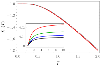
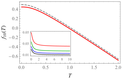
Figure 1: Left: free energy per site of the $\mathrm{su}(1|1)$ PF chain with $\mu_{1}\equiv\mu=K>0$ for $N=10$ spins, $f_{10}(T)$, as a function of $T$ (solid red line) compared to its thermodynamic limit computed via Eq. (5.11) (dashed gray line). Right: same plot for $\mu=-K$. Insets: difference $f(T)-f_{N}(T)$ for $N=10$ (red), $15$ (green), $20$ (blue) and $25$ (black) spins in the range $0\leqslant T\leqslant 10$. Note: in all plots, $f_{N}$, $f$ and $T$ are measured in units of $K$.

5.2 Symmetries of the free energy

We shall next deduce several symmetry properties of the free energy per site $f$ of the Hamiltonian (2.4)–(2.7) stemming from Eqs. (2.9) and (2.10), which shall be frequently applied in the following sections. To this end, in the rest of this section we shall drop the temperature dependence but otherwise use the more descriptive notation $f(\mu_{1},\dots,\mu_{m+n-1};K)$ for the free energy per site. Note, in particular, that the latter notation underscores the fact that we have chosen $\mu_{m+n}=0$ in Eq. (2.4). It is of interest for the sequel to determine how would a different “normalization” of the chemical potentials like, e.g., $\mu_{1}=0$ affect the free energy per site. To see this, let

$$\hat{\mathcal{H}}(\hat{\mu}_{2},\dots,\hat{\mu}_{m+n})={\mathcal{H}}_{0}-\sum_{\alpha=2}^{m+n}\hat{\mu}_{\alpha}{\mathcal{N}}_{\alpha},$$

and denote by $\hat{f}(\hat{\mu}_{2},\dots,\hat{\mu}_{m+n};K)$ the corresponding free energy per site (in the thermodynamic limit). Using the identity

$${\mathcal{N}}_{m+n}=N-\sum_{\alpha=1}^{m+n-1}{\mathcal{N}}_{\alpha}$$

it is straightforward to deduce that

$$\hat{\mathcal{H}}(\hat{\mu}_{2},\dots,\hat{\mu}_{m+n})={\mathcal{H}}(\mu_{1},\dots,\mu_{m+n-1})-N\hat{\mu}_{m+n},$$

where ${\mathcal{H}}(\mu_{1},\dots,\mu_{m+n-1})$ is given by Eq. (2.4) with $\mu_{m+n}=0$ and the chemical potentials $\mu_{\alpha},\hat{\mu}_{\alpha}$ are related by

$$\mu_{\alpha}=\hat{\mu}_{\alpha}-\hat{\mu}_{m+n}\quad(\hat{\mu}_{1}=0)\enspace\iff\enspace\hat{\mu}_{\alpha}=\mu_{\alpha}-\mu_{1}\quad(\mu_{m+n}=0).$$ (5.14)

It then follows that

$$\hat{f}(\hat{\mu}_{2},\dots,\hat{\mu}_{m+n};K)=f(\mu_{1},\dots,\mu_{m+n-1};K)-\hat{\mu}_{m+n}=f(\mu_{1},\dots,\mu_{m+n-1};K)+\mu_{1},$$ (5.15)

with $\mu_{\alpha}$ and $\hat{\mu}_{\alpha}$ related by Eq. (5.14). Consider next Eq. (2.9), which relates the spectra of ${\mathcal{H}}^{(m|n)}$ and ${\mathcal{H}}^{(n|m)}$. Dividing by $N$ and letting $N\to\infty$ we obtain the relation

$$f^{(n|m)}(\mu_{1},\dots,\mu_{m+n-1};K)=\lim_{N\to\infty}\frac{E_{0}}{N}+\hat{f}^{(m|n)}(\mu_{m+n-1},\dots,\mu_{1};-K),$$

where $f^{(n|m)}$ and $\hat{f}^{(m|n)}$ respectively denote the free energy per site of the Hamiltonians ${\mathcal{H}}^{(n|m)}$ (with the usual choice $\mu_{m+n}=0$) and $\hat{\mathcal{H}}^{(m|n)}$ (with $\hat{\mu}_{1}=0$). From Eqs. (2.8), (5.1) and (5.4) we have

$$\lim_{N\to\infty}\frac{E_{0}}{N}=K\lim_{N\to\infty}\frac{1}{N}\sum_{i=1}^{N-1}\varepsilon(x_{i})=K\int_{0}^{1}\varepsilon(x)\rmd x\equiv K\varepsilon_{0}\,,$$

where

$$\varepsilon_{0}=\cases{{\textstyle\frac{1}{6}}\,,&for the HS chain\\ {\textstyle\frac{1}{2}}\,,&for the PF chain\\ {\textstyle\frac{1}{3}}+{\textstyle\frac{\gamma}{2}}\,,&for the FI chain.}$$ (5.16)

Using Eq. (5.15) we finally obtain the remarkable relation

$$f^{(n|m)}(\mu_{1},\dots,\mu_{m+n-1};K)=K\varepsilon_{0}-\mu_{1}+f^{(m|n)}(-\mu_{1},\mu_{m+n-1}-\mu_{1},\dots,\mu_{2}-\mu_{1};-K).$$ (5.17)

Similarly, from Eq. (2.10) we immediately deduce that

$$f(\dots,\mu_{\alpha},\dots,\mu_{\alpha^{\prime}},\dots;K)=f(\dots,\mu_{\alpha^{\prime}},\dots,\mu_{\alpha},\dots;K)\qquad(\pi(\alpha)=\pi(\alpha^{\prime})),$$ (5.18)

so that $f$ is invariant under permutations of chemical potentials of the same type (bosonic or fermionic). Using the latter identity the relation (5.17) can be generalized as follows:

$$f^{(n|m)}(\mu_{1},\dots,\mu_{m+n-1};K)= K\varepsilon_{0}-\mu_{\alpha_{1}}$$ (5.19)

$$+f^{(m|n)}(-\mu_{\alpha_{1}},\mu_{\alpha_{m+n-1}}-\mu_{\alpha_{1}},\dots,\mu_{\alpha_{2}}-\mu_{\alpha_{1}};-K),$$

where $(\alpha_{1},\dots,\alpha_{m+n-1})$ is a permutation of $(1,\dots,m+n-1)$ such that $\{\alpha_{1},\dots,\alpha_{n}\}=\{1,\dots,n\}$.

5.3 Thermodynamic functions

Once the free energy per site is known, all the remaining thermodynamic functions can be easily derived through standard formulas. For instance, the density of $\mathrm{su}(m|n)$ spins of type $\alpha$ (with $\alpha=1,\dots,m+n-1$) is given by

$$n_{\alpha}=-\frac{\partial f}{\partial\mu_{\alpha}}.$$ (5.20)

Indeed, note that if $N_{\alpha}$ (with $\alpha=1,\dots,m+n$) are nonnegative integers such that $N_{1}+\cdots+N_{m+n}=N$, the Hamiltonian ${\mathcal{H}}_{0}$ leaves invariant the subspace ${\mathcal{N}}(N_{1},\dots,N_{m+n})\equiv{\mathcal{N}}(\mathbf{N})$ on which ${\mathcal{N}}_{\alpha}=N_{\alpha}$ for all $\alpha$. Thus the partition function of the chain (2.4) can be written as (recall that we are setting $\mu_{m+n}=0$)

$${\mathcal{Z}}=\sum_{N_{1}+\cdots+N_{m+n}=N}\rme^{\beta\sum\limits_{\alpha=1}^{\mathchoice{\hbox to0.0pt{\hss$\displaystyle{m+n-1}$\hss}}{\hbox to0.0pt{\hss$\textstyle{m+n-1}$\hss}}{\hbox to0.0pt{\hss$\scriptstyle{m+n-1}$\hss}}{\hbox to0.0pt{\hss$\scriptscriptstyle{m+n-1}$\hss}}}\mu_{\alpha}N_{\alpha}}{\mathcal{Z}}_{\mathbf{N}}\,,\qquad\qquad\beta\equiv 1/T\,,$$ (5.21)

where ${\mathcal{Z}}_{\mathbf{N}}$ is the partition function of the restriction of ${\mathcal{H}}_{0}$ to ${\mathcal{N}}(\mathbf{N})$, and is thus independent of the $\mu_{\alpha}$. Hence the thermal average of ${\mathcal{N}}_{\alpha}$ is given by

$$\langle{\mathcal{N}}_{\alpha}\rangle=\frac{1}{{\mathcal{Z}}}\sum_{N_{1}+\cdots+N_{m+n}=N}N_{\alpha}\rme^{\beta\sum\limits_{\alpha=1}^{\mathchoice{\hbox to0.0pt{\hss$\displaystyle{m+n-1}$\hss}}{\hbox to0.0pt{\hss$\textstyle{m+n-1}$\hss}}{\hbox to0.0pt{\hss$\scriptstyle{m+n-1}$\hss}}{\hbox to0.0pt{\hss$\scriptscriptstyle{m+n-1}$\hss}}}\mu_{\alpha}N_{\alpha}}{\mathcal{Z}}_{\mathbf{N}}=T\,\frac{\partial\log{\mathcal{Z}}}{\partial\mu_{\alpha}}\,,$$

which immediately yields Eq. (5.20) for $n_{\alpha}\equiv\langle{\mathcal{N}}_{\alpha}\rangle/N$. Note that this result supports a natural conjecture [40] according to which all the eigenstates $\psi_{k}({\boldsymbol{\sigma}})$ of a supersymmetric $\mathrm{su}(m|n)$ chain of HS type corresponding to an energy $E({\boldsymbol{\sigma}})$ are of the form

$$\psi_{k}({\boldsymbol{\sigma}})=\sum_{P\in{\mathcal{S}}_{N}}c_{P}(k,{\boldsymbol{\sigma}})P|\sigma_{1}\cdots\sigma_{N}\rangle\,,$$

where ${\mathcal{S}}_{N}$ denotes the permutation group of $N$ elements and the coefficients $c_{P}(k,{\boldsymbol{\sigma}})$ are suitable complex numbers. In other words, the number of spins of each type $\alpha$ in the eigenstate $\psi_{K}({\boldsymbol{\sigma}})$ should coincide with the number $N_{\alpha}({\boldsymbol{\sigma}})$ of components of the multiindex ${\boldsymbol{\sigma}}$ equal to $\alpha$. Indeed, if the latter conjecture were true the density $n_{\alpha}$ would be given by

$$n_{\alpha}=\frac{1}{N{\mathcal{Z}}}\sum_{{\boldsymbol{\sigma}}}N_{\alpha}({\boldsymbol{\sigma}})\rme^{-\beta E({\boldsymbol{\sigma}})}\,,$$

where $E({\boldsymbol{\sigma}})$, which is defined by Eq. (4.9), can be alternatively written as

$$E({\boldsymbol{\sigma}})=E^{(m|n)}({\boldsymbol{\sigma}})-\sum_{\alpha^{\prime}=1}^{m+n}\mu_{\alpha^{\prime}}N_{\alpha^{\prime}}({\boldsymbol{\sigma}})\,.$$

Since $E^{(m|n)}({\boldsymbol{\sigma}})$ is independent of the $N_{\alpha^{\prime}}$’s, from the latter equation it follows that

$$n_{\alpha}=\frac{T}{N{\mathcal{Z}}}\,\frac{\partial}{\partial\mu_{\alpha}}\sum_{{\boldsymbol{\sigma}}}\rme^{-\beta E({\boldsymbol{\sigma}})}=\frac{T}{N}\frac{\partial\log{\mathcal{Z}}}{\partial\mu_{\alpha}}=-\frac{\partial f}{\partial\mu_{\alpha}},$$

which coincides with Eq. (5.20).

The variance (per site) of the number of spins of type $\alpha$

$$\nu_{\alpha}\equiv\frac{1}{N}\Big{(}\langle{\mathcal{N}}_{\alpha}^{\,2}\rangle-\langle{\mathcal{N}}_{\alpha}\rangle^{2}\Big{)}$$ (5.22)

can be similarly computed from Eq. (5.21), with the result

$$\nu_{\alpha}=-\beta^{-1}\frac{\partial^{2}f}{\partial\mu_{\alpha}^{2}}\,.$$ (5.23)

The internal energy, heat capacity (at constant volume) and entropy per site are respectively given by the usual formulas

$$u=\frac{\partial}{\partial\beta}(\beta f),\qquad c_{V}=-\beta^{2}\frac{\partial u}{\partial\beta}\,,\qquad s=\beta^{2}\,\frac{\partial f}{\partial\beta}=\beta(u-f)\,.$$ (5.24)

The symmetry properties of the free energy derived in the previous subsection yield analogous properties of the thermodynamic functions just reviewed. For instance, it follows immediately from Eq. (5.18) that the thermodynamic functions $u$, $c_{V}$ and $s$ are invariant under permutations of chemical potentials of the same type, while the particle densities $n_{\alpha}$ (with $\alpha=1,\dots,m+n-1$) behave as

$$n_{\alpha}(\dots,\mu_{\alpha^{\prime}},\dots,\mu_{\alpha^{\prime\prime}},\dots;K)=n_{\alpha}(\dots,\mu_{\alpha^{\prime\prime}},\dots,\mu_{\alpha^{\prime}},\dots;K)\qquad(\pi(\alpha^{\prime})=\pi(\alpha^{\prime\prime}))$$

for $\alpha\neq\alpha^{\prime},\alpha^{\prime\prime}$ and

$$n_{\alpha}(\dots,\mu_{\alpha},\dots,\mu_{\alpha^{\prime}},\dots;K)=n_{\alpha^{\prime}}(\dots,\mu_{\alpha^{\prime}},\dots,\mu_{\alpha},\dots;K)\qquad(\pi(\alpha)=\pi(\alpha^{\prime}))$$

(similar relations hold for $\nu_{\alpha}$). In view of the last equation, we can restrict ourselves without loss of generality to studying just one bosonic and one fermionic density. Likewise, Eq. (5.17) implies that

$$u^{(n|m)}(\mu_{1},\dots,\mu_{m+n-1};K)=K\varepsilon_{0}-\mu_{1}+u^{(m|n)}(-\mu_{1},\mu_{m+n-1}-\mu_{1},\dots,\mu_{2}-\mu_{1};-K),$$ (5.25)

and similar identities for $c_{V}$ and $s$. As to the boson densities, differentiating (5.17) with respect to $\mu_{1}$ we obtain

$$n_{1}^{(n|m)}(\mu_{1},\dots,\mu_{m+n-1};K) =1-\sum_{\alpha=1}^{m+n-1}n_{\alpha}^{(m|n)}(-\mu_{1},\mu_{m+n-1}-\mu_{1},\dots,\mu_{2}-\mu_{1};-K)$$ (5.26)

$$=n_{m+n}^{(m|n)}(-\mu_{1},\mu_{m+n-1}-\mu_{1},\dots,\mu_{2}-\mu_{1};-K)\,.$$

On the other hand, differentiation of Eq. (5.17) with respect to $\mu_{\alpha}$ with $\alpha=2,\dots,m+n-1$ yields

$$n_{\alpha}^{(n|m)}(\mu_{1},\dots,\mu_{m+n-1};K)=n_{m+n+1-\alpha}^{(m|n)}(-\mu_{1},\mu_{m+n-1}-\mu_{1},\dots,\mu_{2}-\mu_{1};-K)\,.$$ (5.27)

Note that the latter equation is actually valid for $\alpha=1,\dots,m+n$, on account of Eq. (5.26) and the identity $n_{m+n}=1-\sum_{\alpha=1}^{m+n-1}n_{\alpha}$. Of course, similar relations hold for the variances per site $\nu_{\alpha}$. In particular, when $m=n$ Eqs. (5.25) (and its analogues for $c_{V}$ and $s$) and (5.27) imply that we can restrict ourselves without loss of generality to positive values of $K$.

In Sections 6–8 we shall apply the results of this section to study the thermodynamics of the $\mathrm{su}(1|1)$, $\mathrm{su}(2|1)$ (or, equivalently, $\mathrm{su}(1|2)$) and $\mathrm{su}(2|2)$ supersymmetric chains (2.4)–(2.7).

6 The $\mathrm{su}(1|1)$ chains

6.1 Free energy per site

In this case the transfer matrix $A(x)$ is simply

$$A(x)=\left(\begin{array}[]{cc}q^{-\mu}&q^{-\frac{\mu}{2}}\\ q^{K\varepsilon(x)-\frac{\mu}{2}}&q^{K\varepsilon(x)}\end{array}\right),\qquad\mu\equiv\mu_{1}\,,$$

with eigenvalues zero and

$$\lambda_{1}(x)=q^{K\varepsilon(x)}+q^{-\mu}\,.$$

In particular, the matrix $A(x)$ is diagonalizable for all $x\in[0,1]$, and condition i) in the previous section is thus trivially satisfied. Condition ii) is also easily verified, as we can simply take

$$P(x)=\left(\begin{array}[]{cc}q^{-(K\varepsilon(x)+\frac{\mu}{2})}&-q^{\frac{\mu}{2}}\\ 1&1\end{array}\right)$$

and therefore

$$\sum_{\alpha=1}^{2}(-1)^{\alpha+1}M_{\alpha 1}(1)q^{-\frac{1}{2}\mu_{\alpha}}=\left|\begin{array}[]{cc}q^{-\frac{\mu}{2}}&-q^{\frac{\mu}{2}}\\ 1&1\end{array}\right|=q^{-\frac{\mu}{2}}+q^{\frac{\mu}{2}}>0.$$

Thus the free energy per site is given by Eq. (5.11), which in this case reads

$$f(T,\mu)=-T\int_{0}^{1}\log\bigl{(}q^{K\varepsilon(x)}+q^{-\mu}\bigr{)}\rmd x=-\mu-\frac{1}{\beta}\int_{0}^{1}\log\Bigl{(}1+\rme^{-\beta(K\varepsilon(x)+\mu)}\Bigr{)}\rmd x\,.$$ (6.1)

For the $\mathrm{su}(1|1)$ HS chain (2.4)-(2.5), Eq. (6.1) coincides with the formula derived in Ref. [34]. The derivation of Eq. (6.1) in the latter reference is based on the equivalence of the $\mathrm{su}(1|1)$ HS chain to a translation-invariant free fermion model, which in turn relies on the symmetry of its dispersion relation $\varepsilon(x)=x(1-x)$ about $x=1/2$. This derivation is therefore not valid for the PF and FI chains, as their dispersion relations are monotonic. The approach followed in this paper circumvents this problem since, as remarked in the previous section, Eq. (6.1) is actually valid for the three chains of HS type (2.5)–(2.7).

As explained in the previous section, since $m=n=1$ we can restrict ourselves in this case to positive values of $K$. This also follows directly from the alternative expression for the free energy per site

$$f=\frac{1}{2}(K\varepsilon_{0}-\mu)-\frac{1}{\beta}\int_{0}^{1}\log\Big{[}2\cosh\Bigl{(}{\textstyle\frac{\beta}{2}}(K\varepsilon(x)+\mu)\Bigr{)}\Big{]}\rmd x\,,$$

which implies (temporarily dropping the dependence of $f$ on the temperature) that

$$f(-\mu;-K)=f(\mu;K)+\mu-K\varepsilon_{0}$$

(cf. Eq. (5.17)).

6.2 Thermodynamic functions

From Eqs. (5.24) and (6.1) we immediately obtain the following explicit formulas for the main thermodynamic functions of the $\mathrm{su}(1|1)$ chains of HS type:

$$n_{1} =\int_{0}^{1}\frac{\rmd x}{1+\rme^{-\beta(K\varepsilon(x)+\mu)}}\,,$$ (6.2)

$$\nu_{1} =\frac{1}{4}\int_{0}^{1}\mathop{\rm sech}\nolimits^{2}\bigl{[}{\textstyle\frac{\beta}{2}}(K\varepsilon(x)+\mu)\bigr{]}\rmd x\,,$$ (6.3)

$$u =-\mu+\int_{0}^{1}\frac{K\varepsilon(x)+\mu}{1+\rme^{\beta(K\varepsilon(x)+\mu)}}\,\rmd x\,,$$ (6.4)

$$c_{V} =\frac{\beta^{2}}{4}\int_{0}^{1}(K\varepsilon(x)+\mu)^{2}\mathop{\rm sech}\nolimits^{2}\bigl{[}{\textstyle\frac{\beta}{2}}(K\varepsilon(x)+\mu)\bigr{]}\rmd x\,,$$ (6.5)

$$s =\int_{0}^{1}\bigg{\{}\log\Bigl{[}2\cosh\bigl{(}{\textstyle\frac{\beta}{2}}(K\varepsilon(x)+\mu)\bigr{)}\Bigr{]}-\frac{\beta}{2}\,(K\varepsilon(x)+\mu)\tanh\bigl{(}{\textstyle\frac{\beta}{2}}(K\varepsilon(x)+\mu)\bigr{)}\bigg{\}}\,\rmd x\,.$$ (6.6)

In Fig. 2 we present a plot of the internal energy, specific heat and entropy per site as a function of $T$ for the three $\mathrm{su}(1|1)$ chains of HS type with $\mu=1/2$. In fact, we have found that the latter functions have the same qualitative behavior for a wide range of values of $\mu$, which is essentially the same as their $\mathrm{su}(2|0)$ counterparts analyzed in Ref. [33]. In particular, the specific heat exhibits the so called Schottky peak, characteristic of two-level systems like the Ising model at zero magnetic field or paramagnetic spin $1/2$ anyons [41].

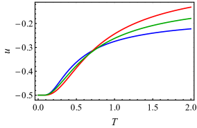
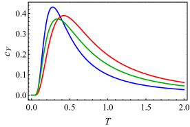
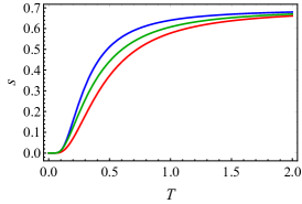
Figure 2: Internal energy (left), specific heat (center) and entropy (right) per site versus the temperature for the HS (blue), PF (red) and FI (with $\gamma=0$, green) $\mathrm{su}(1|1)$ chains with $\mu/K=1/2$. (The internal energy, specific heat and temperature are measured in units of $K$.)

As was the case for the $\mathrm{su}(2|0)$ PF chain studied in Ref. [33], it turns out that the thermodynamic functions of the $\mathrm{su}(1|1)$ PF chain (2.4)-(2.6) can be expressed in closed form in terms of elementary or well-known special functions. To this end, recall first of all the definition of the dilogarithm function [42, 43]

$$\mathop{\rm Li}\nolimits_{2}(z)=-\int_{0}^{z}\frac{\log(1-t)}{t}\,\rmd t,$$ (6.7)

where $\log z$ denotes the determination of the logarithm with $\mathop{\rm Im}\nolimits\log z\in(-\pi,\pi)$ and the integral is taken along any path not intersecting the branch cut on the half-line $[1,\infty)$. Performing the change of variables $t=-\rme^{-\beta(Kx+\mu)}$ in Eq. (6.1) for the PF chain we immediately obtain

$$f(T,\mu)=-\mu+\frac{1}{K\beta^{2}}\Big{[}\mathop{\rm Li}\nolimits_{2}(-\rme^{-\beta\mu})-\mathop{\rm Li}\nolimits_{2}(-\rme^{-\beta(K+\mu)})\Big{]}\,.$$ (6.8)

Differentiation of this expression with respect to $\mu$ yields a remarkable closed formula in terms of elementary functions for the density of bosons of the $\mathrm{su}(1|1)$ PF chain, namely

$$n_{1}=1-\frac{1}{K\beta}\,\log\biggl{(}\frac{1+\rme^{-\beta\mu}}{1+\rme^{-\beta(K+\mu)}}\biggr{)}.$$ (6.9)

The remaining thermodynamic functions admit similar closed-form expressions, namely

$$\nu_{1} =\frac{1}{K\beta}\,\frac{\rme^{-\beta\mu}(1-\rme^{-\beta K})}{(1+\rme^{-\beta\mu})(1+\rme^{-\beta(K+\mu)})}\,,$$ (6.10)

$$u =\frac{\mu}{K\beta}\log(1+\rme^{-\beta\mu})-\frac{K+\mu}{K\beta}\,\log(1+\rme^{-\beta(K+\mu)})-f-2\mu\,,$$ (6.11)

$$c_{V} =\frac{2\mu}{K}\log(1+\rme^{-\beta\mu})-\frac{2(K+\mu)}{K}\log(1+\rme^{-\beta(K+\mu)})$$ (6.12)

$$\hphantom{=\frac{2\mu}{K}\log}{}+\frac{\beta\mu^{2}}{K(1+\rme^{\beta\mu})}-\frac{\beta(K+\mu)^{2}}{K(1+\rme^{\beta(K+\mu)})}\,-2\beta(f+\mu),$$

$$s =\beta(u-f)\,.$$ (6.13)

6.3 Critical behavior

We shall next determine the low temperature behavior of the free energy per site (6.1) for the three HS-types chains (2.5)–(2.7). As is well known, when $T\to 0$ the free energy per unit length of a ($1+1$)-dimensional CFT (in natural units $\hbar=k_{\mathrm{B}}=1$) behaves as

$$f(T)\simeq f(0)-\frac{\pi cT^{2}}{6v}\,,$$ (6.14)

where $c$ is the central charge and $v$ is the effective speed of light [44, 45]. Since the value of $f$ at small temperatures is determined by the low energy excitations, the validity of Eq. (6.14) is generally taken as a strong indication of the conformal invariance of a quantum system. In fact, the latter equation is one of the standard methods for identifying the central charge of the Virasoro algebra of a quantum critical system.

Let us suppose, to begin with, that the boson chemical potential $\mu$ is strictly positive. In this case $K\varepsilon(x)+\mu>0$ for all $x\in[0,1]$ (since, as remarked above, we are taking $K>0$ throughout this section), so that $f(0,\mu)=-\mu$ and

$$|f(T,\mu)-f(0,\mu)|<T\int_{0}^{1}\rme^{-\beta(K\varepsilon(x)+\mu)}<T\rme^{-\beta\mu}\,,$$

so that the system is not critical. A similar result holds for $\mu<-K\varepsilon_{\mathrm{max}}$, where

$$\varepsilon_{\mathrm{max}}=\max_{0\leqslant x\leqslant 1}\varepsilon(x)=\cases{{\textstyle\frac{1}{4}}\,,&for the HS chain\\ 1\,&for the PF chain\\ 1+\gamma,&for the FI chain.}$$

Consider next the case $-K\varepsilon_{\mathrm{max}}<\mu<0$. It is now convenient to rewrite Eq. (6.1) as

$$f(T,\mu)+\mu=-\eta T\int_{0}^{1/\eta}\log\Bigl{(}1+\rme^{-\beta(K\varepsilon(x)+\mu)}\Bigr{)}\rmd x\,,$$ (6.15)

where

$$\eta=\cases{2\,,&for the HS chain\\ 1,&for the PF and FI chains.}$$

This is certainly possible, since the dispersion relation $\varepsilon(x)=x(1-x)$ is symmetric about $x=1/2$. Let $x_{0}$ denote the unique root of the equation $K\varepsilon(x)+\mu=0$ in the interval $(0,1/\eta)$, namely

$$x_{0}=\cases{{\textstyle\frac{1}{2}}\,(1-\sqrt{1+{\textstyle\frac{4\mu}{K}}}\,),&for the HS chain\\ -{\textstyle\frac{\mu}{K}},&for the PF chain\\ {\textstyle\frac{1}{2}}\,(-\gamma+\sqrt{\gamma^{2}-{\textstyle\frac{4\mu}{K}}}\,),&for the FI chain.}$$ (6.16)

Since $K\varepsilon(x)+\mu$ is negative for $0\leqslant x<x_{0}$ and positive for $x_{0}<x\leqslant 1/\eta$, we have

$$f(0,\mu)+\mu=\eta\bigg{(}K\int_{0}^{x_{0}}\varepsilon(x)\rmd x+\mu x_{0}\bigg{)}$$ (6.17)

and

$$f(T,\mu)-f(0,\mu)=-\eta T\int_{0}^{1/\eta}\log\Bigl{(}1+\rme^{-\beta|K\varepsilon(x)+\mu|}\Bigr{)}\rmd x.$$

If we now fix $\Delta<\min(x_{0},1/\eta-x_{0})$  independent of $T$ and set $A\equiv[0,x_{0}-\Delta]\cup[x_{0}+\Delta,1/\eta]$, the latter integral can be approximated by

$$I(T)\equiv\int_{x_{0}-\Delta}^{x_{0}+\Delta}\log\Bigl{(}1+\rme^{-\beta|K\varepsilon(x)+\mu|}\Bigr{)}\rmd x$$

with an error

$$\int_{A}\log\Bigl{(}1+\rme^{-\beta|K\varepsilon(x)+\mu|}\Bigr{)}\rmd x<\int_{A}\rme^{-\beta|K\varepsilon(x)+\mu|}\rmd x<\rme^{-\beta\kappa}\,,$$

with $\kappa=\min(-\mu-\varepsilon(x_{0}-\Delta),\mu+\varepsilon(x_{0}+\Delta))>0$ independent of $T$ . Performing the change of variables $y=\beta|K\varepsilon(x)+\mu|$ in each of the intervals $[x_{0}-\Delta,x_{0}]$ and $[x_{0},x_{0}+\Delta]$ we obtain

$$I(T)=\frac{T}{K}\bigg{(}\int_{0}^{\beta|K\varepsilon(x_{0}-\Delta)+\mu|}\frac{\log(1+\rme^{-y})}{\varepsilon^{\prime}(x)}\,\rmd y+\int_{0}^{\beta|K\varepsilon(x_{0}+\Delta)+\mu|}\frac{\log(1+\rme^{-y})}{\varepsilon^{\prime}(x)}\,\rmd y\bigg{)}.$$ (6.18)

Moreover, since $\varepsilon^{\prime}$ does not vanish on $[x_{0}-\Delta,x_{0}+\Delta]$ we have

$$\frac{1}{\varepsilon^{\prime}(x)}=\frac{1}{\varepsilon^{\prime}(x_{0})}+\Or(x-x_{0})=\frac{1}{\varepsilon^{\prime}(x_{0})}+\Or(Ty),$$ (6.19)

and therefore (taking into account that $\int_{0}^{\infty}y\log(1+\rme^{-y})\rmd y$ is convergent)

$$I(T)=\frac{T}{K\varepsilon^{\prime}(x_{0})}\bigg{(}\int_{0}^{\beta|K\varepsilon(x_{0}-\Delta)+\mu|}+\int_{0}^{\beta|K\varepsilon(x_{0}+\Delta)+\mu|}\bigg{)}\log(1+\rme^{-y})\,\rmd y+\Or(T^{2})\,.$$

It can be easily checked that the error incurred by replacing the upper limits in each of the above integrals by $+\infty$ is $\Or(\rme^{-\kappa^{\prime}\beta})$, where again $\kappa^{\prime}$ is a constant independent of the temperature (see, e.g., Ref. [46]). Hence

$$I(T)=\frac{2T}{K\varepsilon^{\prime}(x_{0})}\int_{0}^{\infty}\log(1+\rme^{-y})\,\rmd y+\Or(T^{2})=\frac{\pi^{2}T}{6K\varepsilon^{\prime}(x_{0})}+\Or(T^{2})\,,$$

and therefore

$$f(T,\mu)=f(0,\mu)-\frac{\eta\pi^{2}T^{2}}{6K\varepsilon^{\prime}(x_{0})}+\Or(T^{3})\,.$$

(See Fig. 3 (left) for a graphic comparison of the latter approximation to the exact expression (6.1) for $\mu/K=-\varepsilon_{\mathrm{max}}/4$ and $T/K\leqslant 0.3$.)

It was shown in Ref. [34] that the $\mathrm{su}(1|1)$ HS chain (2.4)-(2.5) can be mapped to a translationally invariant system of free fermions with energy-momentum relation $E(p)=K\varepsilon(p/(2\pi))$, where $p\in(0,2\pi)$ is the momentum ($\bmod\,2\pi$). Moreover, at low energies the spectrum of this chain consists of small excitations with momenta around $p_{0}\equiv 2\pi x_{0}$ (or $2\pi-p_{0}$), so that the effective speed of light is given by

$$v=\left.\frac{\rmd E}{\rmd p}\right|_{\mathchoice{\hbox to0.0pt{$\displaystyle{p=2\pi x_{0}}$\hss}}{\hbox to0.0pt{$\textstyle{p=2\pi x_{0}}$\hss}}{\hbox to0.0pt{$\scriptstyle{p=2\pi x_{0}}$\hss}}{\hbox to0.0pt{$\scriptscriptstyle{p=2\pi x_{0}}$\hss}}}\enspace=\frac{K\varepsilon^{\prime}(x_{0})}{2\pi}\qquad(\hbox{\rm for the HS chain})\,.$$

Of course, the situation is quite different for the PF and FI chains, since these systems are not translationally invariant and, in particular, their dispersion relation $\varepsilon(x)$ is not symmetric around $x=1/2$. In this case we must therefore take as energy-momentum relation the symmetric extension of $K\varepsilon(p/\pi)$ around $\pi$, i.e.,

$$E(p)=K\varepsilon(1-|1-p/\pi|)\qquad(\hbox{\rm for the PF and FI chains)}$$ (6.20)

(cf. Fig. 3, right), so that now $p=\pi x$ and the effective speed of light is given by

$$v=\left.\frac{\rmd E}{\rmd p}\right|_{\mathchoice{\hbox to0.0pt{$\displaystyle{p=\pi x_{0}}$\hss}}{\hbox to0.0pt{$\textstyle{p=\pi x_{0}}$\hss}}{\hbox to0.0pt{$\scriptstyle{p=\pi x_{0}}$\hss}}{\hbox to0.0pt{$\scriptscriptstyle{p=\pi x_{0}}$\hss}}}\enspace=\frac{K\varepsilon^{\prime}(x_{0})}{\pi}\qquad(\hbox{\rm for the PF and FI chains)}\,.$$

Note that this implies that in the thermodynamic limit (though not for any finite $N$) the $\mathrm{su}(1|1)$ PF and FI chains are equivalent to a translation-invariant free fermion model with energy-momentum relation (6.20), since under the change of variables $x=p/\pi$ Eq. (6.1) becomes

$$f(T,\mu)=-\mu-\frac{T}{\pi}\int_{0}^{\pi}\log(1+\rme^{-\beta(E(p)+\mu)})\,\rmd p.$$

Thus for all three $\mathrm{su}(1|1)$ chains of HS type we can write

$$v=\frac{K\varepsilon^{\prime}(x_{0})}{\eta\pi}\,,$$ (6.21)

and we can therefore express the asymptotic equation for the free energy per site in the unified way

$$f(T,\mu)=f(0,\mu)-\frac{\pi T^{2}}{6v}+\Or(T^{3})\,,$$ (6.22)

where

$$v=\cases{{\textstyle\frac{K}{2\pi}}\,\sqrt{1+{\textstyle\frac{4\mu}{K}}}\,,&for the HS chain\\ {\textstyle\frac{K}{\pi}}\,,&for the PF chain\\ {\textstyle\frac{K}{\pi}}\,\sqrt{\gamma^{2}-{\textstyle\frac{4\mu}{K}}}\,,&for the FI chain.}$$ (6.23)

Comparing with Eq. (6.14) we conclude that for $-K\varepsilon_{\mathrm{max}}<\mu<0$ all of these chains are critical, with $c=1$. In other words, the free energy per site of the three $\mathrm{su}(1|1)$ chains of HS type behaves as that of a CFT with central charge $c=1$ (for instance, a free CFT with one bosonic field).

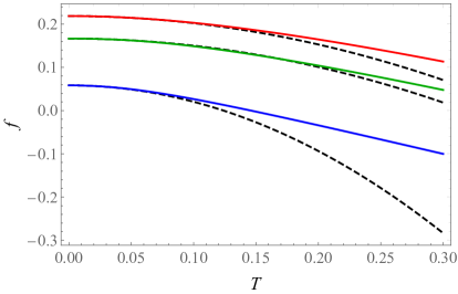
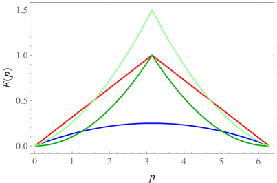
Figure 3: Left: free energy per site versus temperature (both in units of $K$) for the $\mathrm{su}(1|1)$ HS (blue), PF (red) and FI chains (with $\gamma=0$, green) for $\mu/K=-\varepsilon_{\mathrm{max}}/4$. In all three cases, the dashed black line represents the low-temperature approximation (6.22). Right: energy-momentum function $E(p)$ for the $\mathrm{su}(1|1)$ HS (blue), PF (red) and FI chains, with $\gamma=0$ (green) and $\gamma=1/2$ (light green) in the latter case.

For $\mu=0$, a similar analysis shows that the HS, PF and FI (with $\gamma\neq 0$) $\mathrm{su}(1|1)$ chains (2.4)-(2.7) are again critical, but the central charge is now $c=1/2$ (i.e., that of a free CFT with one fermionic field). On the other hand, the FI chain with $\gamma=\mu=0$ is not critical, since following Ref. [46] it can be shown that in this case

$$f(T,0)=-\frac{1}{2}\,\sqrt{\frac{\pi}{K}}\,\bigg{(}1-\frac{1}{\sqrt{2}}\bigg{)}\,\zeta(3/2)\,T^{3/2}+\Or(T^{2}),$$

where $\zeta(z)$ denotes Riemann’s zeta function. Finally, for $\mu=-K\varepsilon_{\mathrm{max}}$ the PF and FI chains are critical with $c=1/2$ (since the root $x_{0}=1$ of $K\varepsilon(x)-K\varepsilon_{\mathrm{max}}$ is simple in both cases), while for the HS chain it was shown in Ref. [34] that

$$f(T,-K/4)=\frac{K}{6}-\sqrt{\frac{\pi}{K}}\,\bigg{(}1-\frac{1}{\sqrt{2}}\bigg{)}\,\zeta(3/2)\,T^{3/2}+\Or(T^{2}).$$

In particular, the $\mathrm{su}(1|1)$ HS chain with $\mu=-K/4$ is not critical. In summary, the phase diagram of the three $\mathrm{su}(1|1)$ chains of HS type is as represented schematically in Fig. 4. For the $\mathrm{su}(1|1)$ HS chain, the above result follows from the general ones in Ref. [34] for a system of spinless free fermions, as well as the direct calculation in Ref. [7]. On the other hand, our result for the $\mathrm{su}(1|1)$ PF chain with $\mu=0$ is in agreement with the heuristic analysis of Ref. [29].

Figure 4: Phase diagram of the $\mathrm{su}(1|1)$ chains of HS type with $K>0$. The critical line and points are colored according to the value of the central charge $c$, as shown in the accompanying legend. The origin is not critical for the FI chain with $\gamma=0$, while the point $-K\varepsilon_{\mathrm{max}}$ is not critical for the HS chain.

6.4 Boson density at low temperatures

The low temperature behavior of the $\mathrm{su}(1|1)$ boson density (6.2) can be analyzed using the results of Ref. [34], which are valid for an arbitrary dispersion function $\varepsilon(x)$. To this end, let us rewrite Eq. (6.2) as

$$n_{1}=\eta\int_{0}^{1/\eta}\frac{\rmd x}{1+\rme^{-\beta(K\varepsilon(x)+\mu)}},$$

so that $\varepsilon(x)$ is monotonically increasing in the interval $[0,1/\eta]$ for all three chains of HS type. It readily follows from the latter expression that the value of the boson density at $T=0$ is given by

$$n_{1}(0,\mu)=\cases{0\,,&\hfill$\mu\leqslant-K\varepsilon_{\mathrm{max}}$\hfill\\ 1-\eta x_{0}\,,&$-K\varepsilon_{\mathrm{max}}\leqslant\mu\leqslant 0$\\ 1\,,&\hfill$\mu\geqslant 0$,\hfill}$$

where $x_{0}$ is given by Eq. (6.16). Thus the $\mathrm{su}(1|1)$ boson density presents a second-order (continuous) phase transition at zero temperature (cf. Fig. 5).

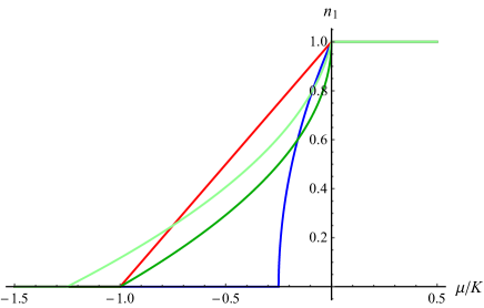
Figure 5: Zero temperature boson density $n_{1}$ as a function of $\mu/K$ for the HS (blue), PF (red) and FI (green for $\gamma=0$, light green for $\gamma=1/4$) chains.

The low temperature behavior of the boson density for the $\mathrm{su}(1|1)$ PF chain follows directly from Eq. (6.9). For instance, in the critical region $-K<\mu<0$ we have

$$n_{1}=1+\frac{\mu}{K}-\mathop{\rm sgn}\nolimits(K+2\mu)\,\frac{T}{K}\,\rme^{-\beta\min(|\mu|,K+\mu)}+\Or\biggl{(}\frac{T}{K}\,\rme^{-\kappa\beta}\biggr{)},$$

with $\kappa=\min(2|\mu|,K+\mu)$ for $-K/2\leqslant\mu<0$ and $\kappa=\min(|\mu|,2K+2\mu)$ for $-K<\mu\leqslant-K/2$. For the HS and FI chains, an asymptotic approximation for $n_{1}$ at low temperatures can be easily derived from the general formulas in Ref. [34]. For instance, in the critical region $-K\varepsilon_{\mathrm{max}}<\mu<0$ we have

$$n_{1} =1-\eta x_{0}+\frac{K\varepsilon^{\prime\prime}(x_{0})}{6\pi\eta^{2}v^{3}}\,T^{2}+\Or(T^{3})$$

$$=\cases{\sqrt{1+{\textstyle\frac{4\mu}{K}}}-{\textstyle\frac{2\pi^{2}}{3K^{2}}}\Big{(}1+{\textstyle\frac{4\mu}{K}}\Big{)}^{-3/2}T^{2}+\Or(T^{3})\,,&for the HS chain\vrule depth=12.0pt,width=0.0pt\\ 1+{\textstyle\frac{1}{2}}\Big{(}\gamma-\sqrt{\gamma^{2}-{\textstyle\frac{4\mu}{K}}}\,\Big{)}+{\textstyle\frac{\pi^{2}}{3K^{2}}}\Big{(}\gamma^{2}-{\textstyle\frac{4\mu}{K}}\Big{)}^{-3/2}T^{2}+\Or(T^{3})\,,&for the FI chain.}$$

The qualitative behavior of the boson density for finite $T$ can also be analyzed with the help of the closed formula (6.2). To begin with, since

$$\frac{\partial n_{1}}{\partial T}=-\frac{\eta}{4T^{2}}\int_{0}^{1/\eta}\frac{K\varepsilon(x)+\mu}{\cosh^{2}\bigl{[}{\textstyle\frac{\beta}{2}}\big{(}K\varepsilon(x)+\mu\big{)}\bigr{]}}\,\rmd x$$

and we are taking $K>0$, it is clear that for $\mu\leqslant-K\varepsilon_{\mathrm{max}}$ (resp. $\mu\geqslant 0$) the boson density increases (resp. decreases) monotonically to its $T\to\infty$ limit $1/2$, as expected. The qualitative behavior of the boson density is more subtle when $\mu$ lies inside the critical interval $(-K\varepsilon_{\mathrm{max}},0)$. To help analyze this behavior, in Fig. 6 (left) we have represented the implicit curve $\frac{\partial n_{1}}{\partial T}=0$ for the three $\mathrm{su}(1|1)$ chains of HS type and $\mu/(K\varepsilon_{\mathrm{max}})$ in the critical range $(-1,0)$. From the latter plot it is clear that for the HS and FI chains there is a range of values of $\mu$ for which $n_{1}$ is not monotonic. More precisely, for the HS chain the boson density has a unique minimum at finite temperature for $-K\varepsilon_{\mathrm{max}}<\mu<\mu_{c}$ for a certain critical chemical potential $\mu_{c}$, since $n_{1}$ is decreasing to the right of the curve $\frac{\partial n_{1}}{\partial T}=0$ and decreasing to its left (this is clear from the behavior of $n_{1}$ for $\mu>0$ and $\mu<-K\varepsilon_{\mathrm{max}}$). Similarly, the boson density of the FI chain presents a unique maximum at finite $T$ in the range $\mu_{c}<\mu<0$, where now the critical value $\mu_{c}$ of $\mu$ depends on the chain parameter $\gamma$. The situation is totally different for the PF chain, for which $n_{1}$ is monotonically increasing (resp. decreasing) for $-K<\mu<-K/2$ (resp. $-K/2<\mu<0$), since now $n_{1}$ is constant for $\mu=-K/2\equiv\mu_{c}$ (cf. Fig. 6, left). The critical chemical potential $\mu_{c}$ can be computed in all cases from the condition

$$\lim_{T\to\infty}T^{2}\frac{\partial n_{1}}{\partial T}(T,\mu_{c})=-\frac{1}{4}\,(K\varepsilon_{0}+\mu_{c})=0\,,$$

which yields $\mu_{c}=-K\varepsilon_{0}$. The qualitative behavior of $n_{1}$ just described is apparent in Fig. 6 (right), where we have plotted the boson density for the three chains of HS type for $\mu=-3K\varepsilon_{\mathrm{max}}/4$ and $\mu=-K\varepsilon_{\mathrm{max}}/4$.

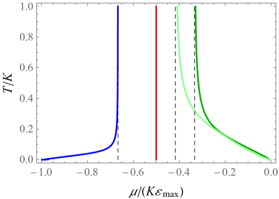
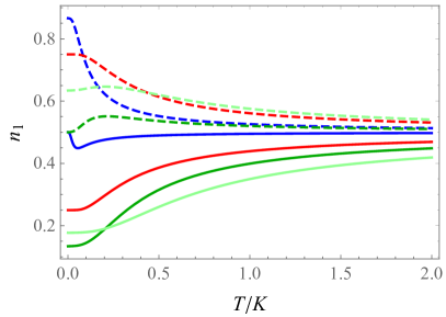
Figure 6: Left: plot of the implicit curve $\frac{\partial n_{1}}{\partial T}=0$ for the $\mathrm{su}(1|1)$ HS (blue), PF (red) and FI chains, with $\gamma=0$ (green) and $\gamma=1$ (light green) in the latter case. The dashed black lines represent the vertical asymptotes $\mu/(K\varepsilon_{\mathrm{max}})=-\varepsilon_{0}/\varepsilon_{\mathrm{max}}=-2/3,-5/12,-1/3$. Right: boson density for $\mu/(K\varepsilon_{\mathrm{max}})=-3/4$ (solid lines) and $\mu/(K\varepsilon_{\mathrm{max}})=-1/4$ (dashed lines), with the same color code.

7 The $\mathrm{su}(2|1)$ chains

This case is of particular interest, since its dual $\mathrm{su}(1|2)$ version with HS interaction (2.5) can be mapped to the spin $1/2$ Kuramoto–Yokoyama $t$-$J$ model in an external magnetic field [47, 48] with a suitable choice of the chemical potentials. In fact, the implications of our results for the latter model (including the discussion of its critical behavior) will be presented in a forthcoming publication. We shall only mention in this regard that, by contrast with the usual approaches, our method does not rely on any approximations and is thus valid for arbitrary temperature.

7.1 Free energy per site

The transfer matrix $A(x)$ is now given by

$$A(x)=\left(\begin{array}[]{ccc}q^{-\mu_{1}}&q^{-\frac{1}{2}(\mu_{1}+\mu_{2})}&-q^{-\frac{\mu_{1}}{2}}\\ q^{K\varepsilon(x)-\frac{1}{2}(\mu_{1}+\mu_{2})}&q^{-\mu_{2}}&q^{-\frac{\mu_{2}}{2}}\\ q^{K\varepsilon(x)-\frac{\mu_{1}}{2}}&q^{K\varepsilon(x)-\frac{\mu_{2}}{2}}&q^{K\varepsilon(x)}\end{array}\right),$$

and its eigenvalues are zero and

$$\lambda_{\pm}(x)=a(x)\pm\sqrt{a(x)^{2}+q^{-(\mu_{1}+\mu_{2})}(q^{K\varepsilon(x)}-1)}\,,$$

where

$$a(x)=\frac{1}{2}\,\Big{(}q^{-\mu_{1}}+q^{-\mu_{2}}+q^{K\varepsilon(x)}\Big{)}\,.$$

Thus the Perron–Frobenius eigenvalue is $\lambda_{1}(x)=\lambda_{+}(x)$. (Note that the term under the square root is clearly positive, since it is strictly greater than $\frac{1}{2}(q^{-\mu_{1}}-q^{-\mu_{2}})^{2}$.) Moreover, the matrix $A(x)$ is again diagonalizable for $0<x<1$, since for these values of $x$ its three eigenvalues are simple on account of the inequality $q^{K\varepsilon(x)}\neq 1$. Hence condition i) of the previous section is again satisfied. Moreover, when $0<x\leqslant 1$ the matrix $P(x)$ for the $\mathrm{su}(2|1)$ PF and FI chains can be taken as

$$P(x)=\left(\begin{array}[]{ccc}q^{\frac{1}{2}(\mu_{2}-\mu_{1})}&0&q^{\frac{1}{2}(\mu_{2}-\mu_{1})}\\[3.0pt] 1+\frac{q^{-\mu_{1}}}{\lambda_{+}(x)}(q^{K\varepsilon(x)}-1)&-q^{\frac{\mu_{2}}{2}}&1+\frac{q^{-\mu_{1}}}{\lambda_{-}(x)}(q^{K\varepsilon(x)}-1)\\[3.0pt] q^{K\varepsilon(x)+\frac{\mu_{2}}{2}}&1&q^{K\varepsilon(x)+\frac{\mu_{2}}{2}}\end{array}\right).$$ (7.1)

Thus Eq. (5.13) in this case reads

$$\left|\begin{array}[]{ccc}q^{-\frac{\mu_{1}}{2}}&0&q^{\frac{1}{2}(\mu_{2}-\mu_{1})}\\[3.0pt] q^{-\frac{\mu_{2}}{2}}&-q^{\frac{\mu_{2}}{2}}&1+\frac{q^{-\mu_{1}}}{\lambda_{-}(1)}(q^{K\varepsilon(1)}-1)\\[3.0pt] 1&1&q^{K\varepsilon(1)+\frac{\mu_{2}}{2}}\end{array}\right|=\frac{q^{-\frac{\mu_{1}}{2}+\mu_{2}}}{\lambda_{-}(1)}\,(1-q^{K\varepsilon(1)})\Big{(}\lambda_{-}(1)+q^{-(\mu_{1}+\mu_{2})}\Big{)}\neq 0.$$

For the PF and FI chains $\varepsilon(1)=1$ and $\varepsilon(1)=1+\gamma\geqslant 1$, respectively, so that the second factor never vanishes. The last one is positive, since it can be written as $\rho-\sqrt{\rho^{2}-\nu}$ with

$$\rho =\frac{1}{2}\,(q^{-\mu_{1}}+q^{-\mu_{2}}+2q^{-(\mu_{1}+\mu_{2})}+q^{K\varepsilon(1)})>0,$$

$$\nu =q^{-2(\mu_{1}+\mu_{2})}+q^{-(\mu_{1}+2\mu_{2})}+q^{-(2\mu_{1}+\mu_{2})}+q^{-(\mu_{1}+\mu_{2})}>0.$$

Thus condition ii) is also satisfied in this case. Applying Eq. (5.11) we then obtain, after a slight simplification,

$$f(T,\mu_{1},\mu_{2})=-\frac{1}{2}(\mu_{1}+\mu_{2})-T\int_{0}^{1}\log\Bigl{(}b(x)+\sqrt{b(x)^{2}+\rme^{-K\beta\varepsilon(x)}-1}\,\Bigr{)}\rmd x,$$ (7.2)

with

$$b(x)=\frac{1}{2}\,\rme^{-\beta[K\varepsilon(x)+\frac{1}{2}(\mu_{1}+\mu_{2})]}+\cosh\Bigl{(}{\textstyle\frac{\beta}{2}}(\mu_{1}-\mu_{2})\Bigr{)}.$$ (7.3)

Comparing the expressions for the eigenvalue $\lambda_{1}(x)=\lambda_{+}(x)$ from the $\mathrm{su}(1|1)$ and $\mathrm{su}(2|1)$ cases we conclude that the $\mathrm{su}(1|1)$ thermodynamic functions can be formally obtained from the $\mathrm{su}(2|1)$ ones in the limit $\mu_{2}\to-\infty$, as expected. The thermodynamic functions of the $\mathrm{su}(2|1)$ chains can be computed without difficulty from Eqs. (7.2)-(7.3) and the general equations (5.20), (5.23) and (5.24), although the corresponding expressions are rather cumbersome and shall therefore not be displayed here.

7.2 Critical behavior

With the help of the explicit formula (7.2), we shall next briefly analyze the criticality properties of the $\mathrm{su}(2|1)$ chains of HS type as a function of the chemical potentials and the interaction strength $K$. We shall see that these chains exhibit a richer critical behavior than their $\mathrm{su}(1|1)$ counterparts, both in terms of the complexity of the critical region and the possible values of the central charge.

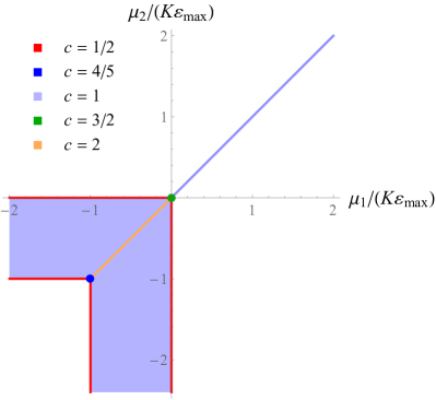
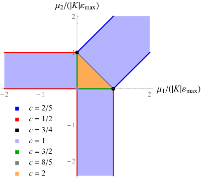
Figure 7: Phase diagram of the $\mathrm{su}(2|1)$ chains of HS type with $K>0$ (left) and $K<0$ (right). The critical regions, lines, and points are colored according to the central charge $c$ as shown in each plot’s legend. For $K>0$, the origin and the half-lines $\mu_{1}=0>\mu_{2}$, $\mu_{2}=0>\mu_{1}$, $\mu_{1}=\mu_{2}>0$ are not critical for the FI chain with $\gamma=0$, while the point $(-K\varepsilon_{\mathrm{max}},-K\varepsilon_{\mathrm{max}})$ and the half-lines $\mu_{1}=-K\varepsilon_{\mathrm{max}}>\mu_{2}$, $\mu_{2}=-K\varepsilon_{\mathrm{max}}>\mu_{1}$ are not critical for the HS chain. Similarly, for $K<0$ the origin and the half-lines $\mu_{1}=0>\mu_{2}$, $\mu_{2}=0>\mu_{1}$, $\mu_{1}=\mu_{2}>0$ are not critical for the FI chain with $\gamma=0$, while the points $(|K|\varepsilon_{\mathrm{max}},0)$, $(0,|K|\varepsilon_{\mathrm{max}})$, the segment $\{\mu_{1}+\mu_{2}=|K|\varepsilon_{\mathrm{max}},\ 0<\mu_{1}<|K|\varepsilon_{\mathrm{max}}\}$ and the half-lines $\{\mu_{1}=|K|\varepsilon_{\mathrm{max}},\ \mu_{2}<0\}$, $\{\mu_{2}=|K|\varepsilon_{\mathrm{max}},\ \mu_{1}<0\}$, $\mu_{1}=\mu_{2}-|K|\varepsilon_{\mathrm{max}}>0$, $\mu_{2}=\mu_{1}-|K|\varepsilon_{\mathrm{max}}>0$ are not critical for the HS chain.

The phase diagram of the $\mathrm{su}(2|1)$ chains is presented in Fig. 7, both for positive and negative values of $K$. For the sake of conciseness, we shall only present the calculations for a few cases of special interest (the remaining ones can be analyzed in a similar fashion). Note that, by Eq. (5.18), we can assume without loss of generality that $\mu_{1}\geqslant\mu_{2}$.

7.2.1 $K>0$.

Consider first the case $K>0$. To begin with, it is clear that the open region $\mu_{1}>0$, $\mu_{1}>\mu_{2}$ is not critical. Indeed, in this region

$$b(x)\underset{T\to 0+}\simeq\frac{1}{2}\Big{(}1+\rme^{-\beta(K\varepsilon(x)+\mu_{1})}\Big{)}\rme^{\frac{\beta}{2}(\mu_{1}-\mu_{2})}\equiv B(x)\rme^{\frac{\beta}{2}(\mu_{1}-\mu_{2})},$$ (7.4)

where we have discarded the exponentially small term $\rme^{-\beta(\mu_{1}-\mu_{2})/2}/2$. It easily follows that $f(0)=-\frac{1}{2}(\mu_{1}+\mu_{2})-\frac{1}{2}(\mu_{1}-\mu_{2})=-\mu_{1}$, and hence when $T\to 0+$

$$|f(T)-f(0)| \simeq\eta T\int_{0}^{1/\eta}\log\Bigl{[}B(x)+\sqrt{B^{2}(x)+\rme^{-\beta(\mu_{1}-\mu_{2})}(\rme^{-K\beta\varepsilon(x)}-1)}\,\Bigr{]}\rmd x$$

$$\leqslant\eta T\int_{0}^{1/\eta}\log\bigl{[}2B(x)\bigr{]}\,\rmd x\leqslant\eta T\int_{0}^{1/\eta}\rme^{-\beta(K\varepsilon(x)+\mu_{1})}\rmd x\leqslant T\rme^{-\beta\mu_{1}},$$

since $K>0$ by assumption. Similarly, if $-K\varepsilon_{\mathrm{max}}>\mu_{1}>\mu_{2}$ we have

$$b(x)\simeq\frac{1}{2}\Big{(}1+\rme^{\beta(K\varepsilon(x)+\mu_{1})}\Big{)}\rme^{-\frac{\beta}{2}(2K\varepsilon(x)+\mu_{1}+\mu_{2})}\equiv\widehat{B}(x)\rme^{-\frac{\beta}{2}(2K\varepsilon(x)+\mu_{1}+\mu_{2})},$$

so that

$$f(0)=-\frac{1}{2}\,(\mu_{1}+\mu_{2})+\frac{\eta}{2}\int_{0}^{1/\eta}(2K\varepsilon(x)+\mu_{1}+\mu_{2})\rmd x=K\varepsilon_{0}$$

and

$$|f(T)-f(0)| \simeq\eta T\int_{0}^{1/\eta}\log\Bigl{[}\widehat{B}(x)+\sqrt{\widehat{B}^{2}(x)+\rme^{\beta(2K\varepsilon(x)+\mu_{1}+\mu_{2})}(\rme^{-K\beta\varepsilon(x)}-1)}\,\Bigr{]}\rmd x$$

$$\leqslant\eta T\int_{0}^{1/\eta}\log\bigl{[}2\widehat{B}(x)\bigr{]}\,\rmd x\leqslant\eta T\int_{0}^{1/\eta}\rme^{\beta(K\varepsilon(x)+\mu_{1})}\rmd x\leqslant T\rme^{\beta(K\varepsilon_{\mathrm{max}}+\mu_{1})}.$$

Thus the triangular region $-K\varepsilon_{\mathrm{max}}>\mu_{1}>\mu_{2}$ is also noncritical.

Likewise, it can be shown that the open region $\mu_{1}>\mu_{2}$, $-K\varepsilon_{\mathrm{max}}<\mu_{1}<0$ is critical, with central charge $c=1$. To this end, let us denote by $x_{0}$ the unique root of the equation $K\varepsilon(x)+\mu_{1}=0$ in the interval $(0,1/\eta)$. We then have

$$f(T)\simeq-\mu_{1}-\eta T\int_{0}^{1/\eta}\log\Bigl{[}B(x)+\sqrt{B^{2}(x)+\rme^{-\beta(\mu_{1}-\mu_{2})}(\rme^{-K\beta\varepsilon(x)}-1)}\,\Bigr{]}\rmd x,$$

where the last term under the square root tends to $0$ as $T\to 0+$, and $K\varepsilon(x)+\mu_{1}$ is positive for $x_{0}<x\leqslant 1/\eta$. It follows that

$$f(0)=-\mu_{1}+\eta\int_{0}^{x_{0}}(K\varepsilon(x)+\mu_{1})\,\rmd x=\eta K\int_{0}^{x_{0}}\varepsilon(x)\rmd x-\mu_{1}(1-\eta x_{0}),$$

and thus

$$f(T)-f(0)\simeq-T(I_{1}+I_{2})\,,$$

where

$$I_{1} =\eta\int_{0}^{x_{0}}\log\Bigl{[}\widehat{B}(x)+\sqrt{\widehat{B}^{2}(x)+\rme^{\beta(2K\varepsilon(x)+\mu_{1}+\mu_{2})}(\rme^{-\beta K\varepsilon(x)}-1)}\,\Bigr{]}\rmd x,$$ (7.5)

$$I_{2} =\eta\int_{x_{0}}^{1/\eta}\log\Bigl{[}B(x)+\sqrt{B^{2}(x)+\rme^{-\beta(\mu_{1}-\mu_{2})}(\rme^{-K\beta\varepsilon(x)}-1)}\,\Bigr{]}\rmd x.$$ (7.6)

As in Subsection 6.3, the main contribution to both integrals comes from an arbitrarily small neighborhood of $x_{0}$, where $|K\varepsilon(x)+\mu_{1}|$ is small. In such a neighborhood, the remaining terms under the square root are negligible, since their exponents are strictly negative in the whole integration range. We thus have

$$I_{1}\simeq\eta\int_{0}^{x_{0}}\log\Bigl{[}2\widehat{B}(x)\Bigr{]}\rmd x,\qquad I_{2}\simeq\eta\int_{x_{0}}^{1/\eta}\log\Bigl{[}2B(x)\Bigr{]}\rmd x\,.$$

We now perform in each of these integrals the change of variables $y=\beta|K\varepsilon(x)+\mu_{1}|$. Taking into account that in a small neighborhood of $x_{0}$

$$\frac{\eta}{K\varepsilon^{\prime}(x)}=\frac{\eta}{K\varepsilon^{\prime}(x_{0})}+\Or(Ty)=\frac{1}{\pi v}+\Or(Ty)\,,$$

where the effective speed of light $v$ is given by Eq. (6.23) with $\mu=\mu_{1}$, we easily obtain

$$I_{1}\simeq\frac{T}{\pi v}\int_{0}^{\beta|\mu_{1}|}\log\Bigl{(}1+\rme^{-y}\Bigr{)}\rmd y\,,\qquad I_{2}\simeq\frac{T}{\pi v}\int_{0}^{\beta|K\varepsilon_{\mathrm{max}}+\mu_{1}|}\log\Bigl{(}1+\rme^{-y}\Bigr{)}\rmd y$$

up to a term of order $\Or(T)$. Extending both integrals to $+\infty$ (which produces an exponentially small error in $\beta$, as shown in Subsection 6.3) we finally obtain

$$I_{1,2}\simeq\frac{T}{\pi v}\int_{0}^{\infty}\log\Bigl{(}1+\rme^{-y}\Bigr{)}\rmd y=\frac{\pi T}{12v}$$

and therefore

$$f(T)-f(0)\simeq-\frac{\pi T^{2}}{6v}\,.$$

Comparing with Eq. (6.14) we conclude that the open set $\mu_{1}>\mu_{2},-K\varepsilon_{\mathrm{max}}<\mu_{1}<0$ is indeed critical, with central charge $c=1$.

The latter results, together with the symmetry of the free energy under exchange of the bosonic chemical potentials, establish the validity of the phase diagram in Fig. 7 (left) in the “generic” subset $\mu_{1}\neq\mu_{2}$ minus the half-lines $\mu_{1}=0\geqslant\mu_{2}$, $\mu_{2}=0\geqslant\mu_{1}$, $\mu_{1}=-K\varepsilon_{\mathrm{max}}\geqslant\mu_{2}$, $\mu_{2}=-K\varepsilon_{\mathrm{max}}\geqslant\mu_{1}$. To end the discussion for $K>0$, we shall limit ourselves to analyzing the points $(0,0)$ and $(-K\varepsilon_{\mathrm{max}},-K\varepsilon_{\mathrm{max}})$, which illustrate the general procedure.

First of all, at the origin we have

$$f(T)=-\eta T\int_{0}^{1/\eta}\log\Bigl{[}1+{\textstyle\frac{1}{2}}\,\rme^{-K\beta\varepsilon(x)}+\sqrt{2\rme^{-K\beta\varepsilon(x)}+{\textstyle\frac{1}{4}}\,\rme^{-2K\beta\varepsilon(x)}}\,\Bigr{]}\rmd x.$$

Performing again the change of variables $K\beta\varepsilon(x)=y$ and proceeding as above we obtain

$$f(T)\simeq-\frac{T^{2}}{\pi v}\int_{0}^{\infty}\log\Bigl{[}1+{\textstyle\frac{1}{2}}\,\rme^{-y}+\sqrt{2\rme^{-y}+{\textstyle\frac{1}{4}}\,\rme^{-2y}}\,\Bigr{]}\rmd y=-\frac{\pi T^{2}}{4v}\,,$$

where now $v=K\varepsilon^{\prime}(0)/(\eta\pi)$. (Of course, the latter formula is clearly not valid for the FI chain with $\gamma=0$, as $\varepsilon^{\prime}(0)=0$ in this case. In fact, it is straightforward to show that this chain is not critical when $\mu_{1}=\mu_{2}=0$, since $f(T)-f(0)\propto T^{-3/2}$.) Comparing with Eq. (6.14) we conclude that (except for the FI chain with $\gamma=0$) the model is critical in this case with central charge $c=3/2$ (i.e., that of a free CFT with one boson and one fermion). This is again in agreement with the general result of Ref. [29] for the $\mathrm{su}(m|n)$ PF chain with zero chemical potentials, according to which $c=m-1+n/2$ for $m\geqslant 1$. In fact, the same is true for the $\mathrm{su}(1|2)$ chains with $\mu_{1}=\mu_{2}=0$ (excluding again the FI chain with $\gamma=0$). Indeed, using Eq. (5.19) we readily obtain

$$f(T)-f(0)=f(T)-K\varepsilon_{0}\simeq-\frac{T^{2}}{\pi v}\int_{0}^{\infty}\log\Bigl{[}{\textstyle\frac{1}{2}}+\rme^{-y}+\sqrt{{\textstyle\frac{1}{4}}+2\rme^{-y}}\,\Bigr{]}\rmd y=-\frac{\pi T^{2}}{6v},$$

so that $c=1=m-1+n/2$ also in this case.

Consider, finally, the case $\mu_{1}=\mu_{2}=-K\varepsilon_{\mathrm{max}}=-K\varepsilon(1/\eta)\equiv\mu$, for which

$$f(T)=-\mu-\eta T\int_{0}^{1/\eta}\log\Bigl{[}1 +{\textstyle\frac{1}{2}}\,\rme^{-\beta(K\varepsilon(x)+\mu)}$$

$$+\sqrt{\rme^{-\beta(K\varepsilon(x)+\mu)}+{\textstyle\frac{1}{4}}\,\rme^{-2\beta(K\varepsilon(x)+\mu)}+\rme^{-K\beta\varepsilon(x)}}\,\Bigr{]}\rmd x,$$

and hence

$$f(0)=-\mu+\eta\int_{0}^{1/\eta}(K\varepsilon(x)+\mu)\rmd x=K\varepsilon_{0}\,.$$

We thus have

$$f(T)-f(0) =-\eta T\int_{0}^{1/\eta}\log\Bigl{[}{\textstyle\frac{1}{2}}+\rme^{\beta(K\varepsilon(x)+\mu)}+\sqrt{{\textstyle\frac{1}{4}}+\rme^{\beta(K\varepsilon(x)+\mu)}+\rme^{\beta(K\varepsilon(x)+2\mu)}}\,\Bigr{]}\rmd x,$$

$$\simeq-\eta T\int_{0}^{1/\eta}\log\Bigl{[}{\textstyle\frac{1}{2}}+\rme^{\beta(K\varepsilon(x)+\mu)}+\sqrt{{\textstyle\frac{1}{4}}+\rme^{\beta(K\varepsilon(x)+\mu)}}\,\Bigr{]}\rmd x\,,$$

since $\mu<0$. The PF and FI chains both satisfy the condition $\varepsilon^{\prime}(1)\neq 0$. In this case, performing the usual change of variables $\beta(K\varepsilon(x)+\mu)=-y$ and taking into account the definition (6.21) of the effective speed of light $v$ we obtain

$$f(T)-f(0)\simeq-\frac{T^{2}}{\pi v}\int_{0}^{\infty}\log\Bigl{[}{\textstyle\frac{1}{2}}+\rme^{-y}+\sqrt{{\textstyle\frac{1}{4}}+\rme^{-y}}\,\Bigr{]}\rmd y=-\frac{2\pi T^{2}}{15v}\,.$$

Thus the $\mathrm{su}(2|1)$ PF and FI chains with $\mu_{1}=\mu_{2}=-K\varepsilon_{\mathrm{max}}$ are both critical with central charge $c=4/5$, as claimed. Remarkably, this value of $c$ coincides with the central charge of the three-state Potts model [49, 50] (or, indeed, of any unitary minimal model [51] with $p=5$, where $c=1-6/[p(p+1)]$). Obviously, the latter conclusions do not hold for the HS chain, since in this case we have $\varepsilon^{\prime}(1/\eta)=\varepsilon(1/2)=0$. In fact, it can be shown without difficulty that this chain is not critical when $\mu_{1}=\mu_{2}=-K/4$.

7.2.2 $K<0$.

The phase diagram for $K<0$ is more complex than its $K>0$ counterpart, as is apparent from Fig. 7. We shall therefore limit ourselves to discussing the two most interesting cases, namely the half-line $\mu_{2}=\mu_{1}-|K|\varepsilon_{\mathrm{max}}>0$ and the point $(|K|\varepsilon_{\mathrm{max}},0)$. (Note that, by Eq. (5.18), the results we shall obtain automatically apply to the half-line $\mu_{1}=\mu_{2}-|K|\varepsilon_{\mathrm{max}}>0$ and the point $(0,|K|\varepsilon_{\mathrm{max}})$.)

Consider, to begin with, the half-line $\mu_{2}=\mu_{1}-|K|\varepsilon_{\mathrm{max}}>0$, on which

$$b(x)=\frac{1}{2}\Big{(}1+\rme^{\beta(|K|\varepsilon(x)-\mu_{1})}+\rme^{-|K|\beta\varepsilon_{\mathrm{max}}}\Big{)}\rme^{\frac{\beta}{2}|K|\varepsilon_{\mathrm{max}}}\equiv\hat{b}(x)\,\rme^{\frac{\beta}{2}|K|\varepsilon_{\mathrm{max}}}\,,$$ (7.7)

and consequently

$$f(T)=-\mu_{1}-\eta T\int_{0}^{1/\eta}\log\Bigl{[}\hat{b}(x)+\sqrt{\hat{b}(x)^{2}+\rme^{|K|\beta(\varepsilon(x)-\varepsilon_{\mathrm{max}})}-\rme^{-|K|\beta\varepsilon_{\mathrm{max}}}}\,\Bigr{]}\rmd x.$$ (7.8)

Since $\rme^{\beta(|K|\varepsilon(x)-\mu_{1})}\leqslant\rme^{-\beta|K|\mu_{2}}$, the function $\hat{b}(x)$ differs from $1/2$ by terms that are exponentially small in $\beta$. Discarding these terms we obtain the approximation

$$f(T)-f(0)\simeq-\eta T\int_{0}^{1/\eta}\log\Bigl{[}{\textstyle\frac{1}{2}}+\sqrt{{\textstyle\frac{1}{4}}+\rme^{|K|\beta(\varepsilon(x)-\varepsilon_{\mathrm{max}})}}\,\Bigr{]}\rmd x\,,$$

with $f(0)=-\mu_{1}$. We now perform the usual change of variable

$$y=|K|\beta\big{(}\varepsilon_{\mathrm{max}}-\varepsilon(x)\big{)},$$ (7.9)

which yields

$$f(T)-f(0)\simeq-\frac{\eta T^{2}}{|K|}\int_{0}^{|K|\beta\varepsilon_{\mathrm{max}}}\log\Bigl{[}{\textstyle\frac{1}{2}}+\sqrt{{\textstyle\frac{1}{4}}+\rme^{-y}}\,\Bigr{]}\frac{\rmd y}{\varepsilon^{\prime}(x)}\,,$$ (7.10)

where $x$ should be expressed in terms of $y$ inverting Eq. (7.9). As before, we can replace the term $1/\varepsilon^{\prime}(x)$ by its approximation near the lower endpoint of the integral (i.e., near $x=1/\eta$), where the integrand is not exponentially small. For the PF and FI chains $\varepsilon^{\prime}(1/\eta)=\varepsilon^{\prime}(1)\neq 0$, so that we can use Eqs. (6.19) and (6.21) with $x_{0}=\eta=1$. Extending the integral to $+\infty$ (which, as we saw above, produces an exponentially small error) we thus obtain

$$f(T)-f(0)\simeq-\frac{T^{2}}{\pi v}\int_{0}^{\infty}\log\Bigl{[}{\textstyle\frac{1}{2}}+\sqrt{{\textstyle\frac{1}{4}}+\rme^{-y}}\,\Bigr{]}\rmd y=-\frac{\pi T^{2}}{15v}\,.$$

Comparing with Eq. (6.14) we conclude that in this case the PF and FI chains are critical, with $c=2/5$. Interestingly, this value of $c$ does not coincide with the central charge of a minimal unitary model (nor even, to the best of our knowledge, of a nonunitary minimal model).

The situation is quite different for the HS chain, since in this case $\varepsilon^{\prime}(x)$ vanishes at the endpoint $x=1/\eta=1/2$. We now have

$$y=|K|\beta\big{(}{\textstyle\frac{1}{2}}-x\big{)}^{2}\,,\qquad\varepsilon^{\prime}(x)=1-2x=2\,\sqrt{\frac{Ty}{|K|}}\,$$

and hence

$$f(T)-f(0)\simeq-\frac{\kappa T^{3/2}}{\sqrt{|K|}}\,,\qquad\kappa\equiv\frac{1}{4}\int_{0}^{\infty}y^{-1/2}\log\Bigl{[}{\textstyle\frac{1}{2}}+\sqrt{{\textstyle\frac{1}{4}}+\rme^{-y}}\,\Bigr{]}\rmd y\simeq 0.254707\,.$$

Thus the $\mathrm{su}(2|1)$ HS chain with $K<0$ is not critical along the half-line $\mu_{2}=\mu_{1}-|K|\varepsilon_{\mathrm{max}}>0$.

Let us now turn to the point $(|K|\varepsilon_{\mathrm{max}},0)$, i.e., the endpoint of the half-line just considered. Using Eq. (7.8) with

$$\hat{b}(x)=\frac{1}{2}\Big{(}1+\rme^{\beta(|K|(\varepsilon(x)-\varepsilon_{\mathrm{max}})}+\rme^{-|K|\beta\varepsilon_{\mathrm{max}}}\Big{)}$$

(cf. Eq. (7.7)) and discarding the exponentially small term $\rme^{-|K|\beta\varepsilon_{\mathrm{max}}}$ we easily arrive at the asymptotic formula

$$f(T)-f(0)\simeq-\frac{\eta T^{2}}{|K|}\int_{0}^{|K|\beta\varepsilon_{\mathrm{max}}}\log\Bigl{[}{\textstyle\frac{1}{2}}\big{(}1+\rme^{-y}\big{)}+\sqrt{{\textstyle\frac{1}{4}}\,\big{(}1+\rme^{-y}\big{)}^{2}+\rme^{-y}}\,\Bigr{]}\,\frac{\rmd y}{\varepsilon^{\prime}(x)}\,,$$

where $x$ and $y$ are related by the change of variables (7.9). As explained above, for the PF and FI chains we can replace $\varepsilon^{\prime}(x)$ by $\varepsilon^{\prime}(1/\eta)=\varepsilon^{\prime}(1)$ and extend the integral to $+\infty$, obtaining

$$f(T)-f(0)\simeq-\frac{T^{2}}{\pi v}\int_{0}^{\infty}\log\Bigl{[}{\textstyle\frac{1}{2}}\big{(}1+\rme^{-y}\big{)}+\sqrt{{\textstyle\frac{1}{4}}\,\big{(}1+\rme^{-y}\big{)}^{2}+\rme^{-y}}\,\Bigr{]}\,\rmd y=-\frac{\pi T^{2}}{8v}\,,$$

where $v=|K|\,\varepsilon^{\prime}(1)/\pi$. Thus the $\mathrm{su}(2|1)$ PF and FI chains are critical in this case, with $c=3/4$ (cf. Eq. (6.14)). Again, this value of $c$ does not coincide with the central charge of a unitary (or, to the best of our knowledge, nonunitary) minimal model. Finally, for the HS chain proceeding as above we again obtain

$$f(T)-f(0)\simeq-\frac{\kappa T^{3/2}}{\sqrt{|K|}}\,,$$

where now

$$\kappa=\frac{1}{4}\int_{0}^{\infty}y^{-1/2}\log\Bigl{[}{\textstyle\frac{1}{2}}\big{(}1+\rme^{-y}\big{)}+\sqrt{{\textstyle\frac{1}{4}}\,\big{(}1+\rme^{-y}\big{)}^{2}+\rme^{-y}}\,\Bigr{]}\,\rmd y\simeq 0.471976\,.$$

Thus the $\mathrm{su}(2|1)$ HS chain with $K<0$ is not critical at the point $(|K|\varepsilon_{\mathrm{max}},0)$.

7.3 Zero-temperature densities

From Eqs. (5.20) and (7.2)-(7.3) we obtain the following explicit expressions for the particle densities of the $\mathrm{su}(2|1)$ chains of HS type:

$$n_{1}(T,\mu_{1},\mu_{2}) =\frac{1}{2}+\frac{\eta}{2}\,\int_{0}^{1/\eta}\frac{\sinh(\beta\mu_{-})-\frac{1}{2}\rme^{-\beta(K\varepsilon(x)+\mu_{+})}}{\sqrt{b(x)^{2}+\rme^{-K\beta\varepsilon(x)}-1}}\,\rmd x\,,$$ (7.11)

$$n_{2}(T,\mu_{1},\mu_{2}) =n_{1}(T,\mu_{2},\mu_{1})\,,$$ (7.12)

$$n_{3}(T,\mu_{1},\mu_{2}) =\frac{\eta}{2}\,\int_{0}^{1/\eta}\frac{\rme^{-\beta(K\varepsilon(x)+\mu_{+})}}{\sqrt{b(x)^{2}+\rme^{-K\beta\varepsilon(x)}-1}}\,\rmd x\,,$$ (7.13)

with

$$\mu_{\pm}\equiv\frac{1}{2}\,(\mu_{1}\pm\mu_{2})\,.$$

We shall limit ourselves to analyzing the behavior of these densities at zero temperature. By contrast with the $\mathrm{su}(2|0)$ and $\mathrm{su}(1|1)$ cases, we shall show that in this case the bosonic densities exhibit a first-order (discontinuous) phase transition across the half-line $\mu_{1}=\mu_{2}>-K\varepsilon_{\mathrm{max}}$ for $K>0$.

Suppose, to begin with, that $K>0$, and consider first the fermionic density $n_{3}$. Since this density is clearly symmetric under exchange of the bosonic chemical potentials, we shall restrict ourselves without loss of generality to the case $\mu_{1}\geqslant\mu_{2}$. When $\mu_{1}>\mu_{2}$, using the low temperature approximation (7.4) we have

$$n_{3}\simeq\eta\int_{0}^{1/\eta}\Big{[}(1+\rme^{\beta(K\varepsilon(x)+\mu_{1})})^{2}-4\rme^{2\beta(K\varepsilon(x)+\mu_{+})}\Big{]}^{-1/2}\rmd x\,,$$ (7.14)

where we have taken into account that $\rme^{\beta(K\varepsilon(x)+2\mu_{+})}\ll\rme^{2\beta(K\varepsilon(x)+\mu_{+})}$ as $T\to 0+$ for $0<x\leqslant 1/\eta$. When $K\varepsilon(x)+\mu_{1}>0$, the term $\rme^{2\beta(K\varepsilon(x)+\mu_{1})}$ dominates over the remaining ones as $T\to 0+$, so that the integrand tends to zero in this region. On the other hand, when $K\varepsilon(x)+\mu_{1}<0$ the integrand clearly tends to $1$ as $T\to 0+$. We thus have

$$n_{3}(0)=\eta|I(\mu_{1})|\,,$$

where $|I(\mu)|$ denotes the length of the (possibly empty) interval

$$I(\mu)=\{x\in[0,1/\eta]:K\varepsilon(x)+\mu<0\}.$$

Denoting by $x_{0}(\mu)$ the unique root of the equation $K\varepsilon(x)+\mu=0$ in the interval $[0,\eta]$ (cf. Eq. (6.16)), we conclude that for $K>0$ and $\mu_{1}>\mu_{2}$ the zero temperature fermionic density is given by

$$n_{3}(0)=\cases{0,&$\mu_{1}>0,$\\ \eta\,x_{0}(\mu_{1}),&$-K\varepsilon_{\mathrm{max}}\leqslant\mu_{1}\leqslant 0,$\\ 1,&$\mu_{1}<-K\varepsilon_{\mathrm{max}}$\,.}$$

Likewise, for $K>0$ and $\mu_{1}=\mu_{2}\equiv\mu$ we have

$$n_{3}=\eta\int_{0}^{1/\eta}\Big{[}1+4\rme^{\beta(K\varepsilon(x)+\mu)}+4\rme^{\beta(K\varepsilon(x)+2\mu)}\Big{]}^{-1/2}\rmd x\,,$$

so that again $n_{3}(0)=\eta|I(\mu)|$. From the previous formulas and the symmetry of $n_{3}$ under the exchange of $\mu_{1}$ with $\mu_{2}$ we obtain the following expression for $n_{3}(0)$, valid in the whole $(\mu_{1},\mu_{2})$ plane when $K>0$:

$$n_{3}(0)=\cases{0,&$\max(\mu_{1},\mu_{2})>0$,\\ \eta x_{0}(\max(\mu_{1},\mu_{2})),&$-K\varepsilon_{\mathrm{max}}\leqslant\max(\mu_{1},\mu_{2})\leqslant 0$,\\ 1,&$\max(\mu_{1},\mu_{2})<-K\varepsilon_{\mathrm{max}}$\,.}$$ (7.15)

It is apparent from the latter expression that $n_{3}$ is continuous, but its gradient is discontinuous along the segment $-K\varepsilon_{\mathrm{max}}\leqslant\mu_{1}=\mu_{2}\leqslant 0$ and the half-lines $\mu_{1}=0>\mu_{2}$, $\mu_{2}=0>\mu_{1}$, $\mu_{1}=-K\varepsilon_{\mathrm{max}}>\mu_{2}$, $\mu_{2}=-K\varepsilon_{\mathrm{max}}>\mu_{1}$ (cf. Fig. 8, left).

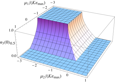
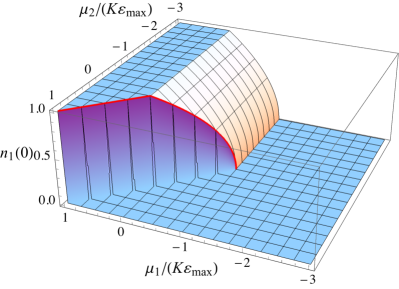
Figure 8: Left: fermion density at zero temperature for the $\mathrm{su}(2|1)$ HS chain with $K>0$. Right: same plot for the bosonic density $n_{1}$, with a red line drawn to illustrate the discontinuity along the half-line $\mu_{1}=\mu_{2}\geqslant-K\varepsilon_{\mathrm{max}}$.

Consider next the density $n_{1}$ of the first species of bosons, which for $\mu_{1}>\mu_{2}$ can be expressed as

$$n_{1}=\frac{1}{2}\,(1-n_{3})+\frac{\eta}{2}\,\int_{0}^{1/\eta}D(x)^{-1/2}\rmd x\,,\qquad D(x)\equiv\frac{b(x)^{2}+\rme^{-K\beta\varepsilon(x)}-1}{\sinh^{2}(\beta\mu_{-})}\,.$$ (7.16)

At low temperatures we have

$$D(x)=\Big{(}1+\rme^{-\beta(K\varepsilon(x)+\mu_{1})}\Big{)}^{2}+\Or(\rme^{-2\beta\mu_{-}}),$$

so that

$$\lim_{T\to 0+}\int_{0}^{1/\eta}D(x)^{-1/2}\rmd x=\Big{|}\{x\in[0,1/\eta]:K\varepsilon(x)+\mu_{1}>0\}\Big{|}=\frac{1}{\eta}-|I(\mu_{1})|,$$

and thus

$$n_{1}(0)=\frac{1}{2}\Big{(}1-n_{3}(0)\Big{)}+\frac{1}{2}\Big{(}1-\eta|I(\mu_{1})|\Big{)}\,.$$

Using the previous formula for $n_{3}(0)$ we obtain the following expression for $n_{1}(0)$ when $K>0$ and $\mu_{1}>\mu_{2}$:

$$n_{1}(0)=\cases{1\,,&$\mu_{1}>0,$\\ 1-\eta\,x_{0}(\mu_{1}),&$-K\varepsilon_{\mathrm{max}}\leqslant\mu_{1}\leqslant 0,$\\ 0,&$\mu_{1}<-K\varepsilon_{\mathrm{max}}$\,.}$$

On the other, when $K>0$ and $\mu_{2}>\mu_{1}$ we have

$$n_{1}=\frac{1}{2}\,(1-n_{3})-\frac{\eta}{2}\,\int_{0}^{1/\eta}D(x)^{-1/2}\rmd x\,,$$

so that proceeding as before we obtain

$$n_{1}(0)=\frac{1}{2}\Big{(}1-n_{3}(0)\Big{)}-\frac{1}{2}\Big{(}1-\eta|I(\mu_{2})|\Big{)}=0\,.$$

Finally, when $\mu_{1}=\mu_{2}$ by Eq. (7.16) we simply have $n_{1}(0)=(1-n_{3}(0))/2$. Taking into account the symmetry of $n_{1}$ under exchange of $\mu_{1}$ with $\mu_{2}$ we obtain the following general expression for the latter density (for $K>0$):

$$n_{1}(0)=\cases{0,&$\mu_{1}<\mu_{2}$ or $-K\varepsilon_{\mathrm{max}}\geqslant\mu_{1}>\mu_{2}$,\\ {\textstyle\frac{1}{2}},&$\mu_{1}=\mu_{2}\geqslant 0,$\\ {\textstyle\frac{1}{2}}(1-\eta x_{0}(\mu_{1})),&$-K\varepsilon_{\mathrm{max}}\leqslant\mu_{1}=\mu_{2}<0,$\\ 1-\eta x_{0}(\mu_{1}),&$-K\varepsilon_{\mathrm{max}}\leqslant\mu_{1}\leqslant 0,\enspace\mu_{1}>\mu_{2}$,\\ 1,&$\mu_{1}>0,\enspace\mu_{1}>\mu_{2}$\,.}$$ (7.17)

It follows from the previous expression that $n_{1}$ is discontinuous along the half-line $\mu_{1}=\mu_{2}\geqslant-K\varepsilon_{\mathrm{max}}$, and has a discontinuous gradient along the half-lines $\mu_{1}=-K\varepsilon_{\mathrm{max}}\geqslant\mu_{2}$ and $\mu_{1}=0\geqslant\mu_{2}$. Thus in this case the bosonic density $n_{1}$ (and hence $n_{2}$) presents both first- and second-order phase transitions for appropriate values of the chemical potentials $\mu_{1}$ and $\mu_{2}$. A very similar calculation, that we shall omit for the sake of conciseness, shows that when $K<0$ the fermionic density is given by

$$n_{3}(0)=\cases{0,&$\mu_{1}-\mu_{2}\geqslant|K|\varepsilon_{\mathrm{max}}$ or $\max(\mu_{1},\mu_{2})\geqslant|K|\varepsilon_{\mathrm{max}}$,\\ 1-\eta x_{0}(\max(\mu_{1},\mu_{2})),&$0\leqslant\max(\mu_{1},\mu_{2})\leqslant|K|\varepsilon_{\mathrm{max}},\;\min(\mu_{1},\mu_{2})\leqslant 0$,\\ 1-\eta x_{0}(\mu_{1}+\mu_{2}),&$\mu_{1}\geqslant 0,\;\mu_{2}\geqslant 0,\;\mu_{1}+\mu_{2}\leqslant|K|\varepsilon_{\mathrm{max}}$,\\ 1,&$\mu_{1}\leqslant 0,\;\mu_{2}\leqslant 0$,}$$

while the bosonic density $n_{1}(0)$ reads

$$n_{1}(0)=$$

$$\cases{0,&$\mu_{1}\leqslant 0$ or $\mu_{2}-\mu_{1}\geqslant|K|\varepsilon_{\mathrm{max}}$,\\ \eta x_{0}(\mu_{1}),&$0\leqslant\mu_{1}\leqslant|K|\varepsilon_{\mathrm{max}},\;\mu_{2}\leqslant 0$,\\ {\textstyle\frac{\eta}{2}}\Big{[}x_{0}(\mu_{1}+\mu_{2})+\mathop{\rm sgn}\nolimits(\mu_{1}-\mu_{2})x_{0}(|\mu_{1}-\mu_{2}|)\Big{]},&$\mu_{1}\geqslant 0,\;\mu_{2}\geqslant 0,\;\mu_{1}+\mu_{2}\leqslant|K|\varepsilon_{\mathrm{max}},$\\ {\textstyle\frac{1}{2}}\Big{[}1+\eta\mathop{\rm sgn}\nolimits(\mu_{1}-\mu_{2})x_{0}(|\mu_{1}-\mu_{2}|)\Big{]},&$|\mu_{1}-\mu_{2}|\leqslant|K|\varepsilon_{\mathrm{max}},\;\mu_{1}+\mu_{2}\geqslant|K|\varepsilon_{\mathrm{max}},$\\ 1,&$\mu_{1}-\mu_{2}\geqslant|K|\varepsilon_{\mathrm{max}},\;\mu_{1}\geqslant|K|\varepsilon_{\mathrm{max}}$\,.}$$

It can be easily checked that both densities (and hence the remaining one $n_{2}(0)$) are continuous, although their gradient is discontinuous along several segments and half-lines (cf. Fig. 9). Thus when $K<0$ the chains (2.4)–(2.7) exhibit only second-order phase transitions at zero temperature.

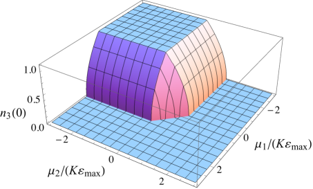
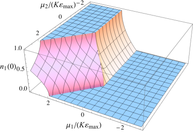
Figure 9: Left: fermion density at zero temperature for the $\mathrm{su}(2|1)$ HS chain with $K<0$. Right: same plot for the bosonic density $n_{1}$.

8 The $\mathrm{su}(2|2)$ chains

The eigenvalues of the $\mathrm{su}(2|2)$ transfer matrix

$$A(x)=\left(\begin{array}[]{cccc}q^{-\mu_{1}}&q^{-\frac{1}{2}(\mu_{1}+\mu_{2})}&q^{-\frac{1}{2}(\mu_{1}+\mu_{3})}&q^{-\frac{\mu_{1}}{2}}\\ q^{K\varepsilon(x)-\frac{1}{2}(\mu_{1}+\mu_{2})}&q^{-\mu_{2}}&q^{-\frac{1}{2}(\mu_{2}+\mu_{3})}&q^{-\frac{\mu_{2}}{2}}\\ q^{K\varepsilon(x)-\frac{1}{2}(\mu_{1}+\mu_{3})}&q^{K\varepsilon(x)-\frac{1}{2}(\mu_{2}+\mu_{3})}&q^{K\varepsilon(x)-\mu_{3}}&q^{-\frac{\mu_{3}}{2}}\\ q^{K\varepsilon(x)-\frac{\mu_{1}}{2}}&q^{K\varepsilon(x)-\frac{\mu_{2}}{2}}&q^{K\varepsilon(x)-\frac{\mu_{3}}{2}}&q^{K\varepsilon(x)}\end{array}\right)$$

are zero (double) and

$$\lambda_{\pm}(x)=a(x)\pm\sqrt{a(x)^{2}+(q^{K\varepsilon(x)}-1)(q^{-(\mu_{1}+\mu_{2})}-q^{K\varepsilon(x)-\mu_{3}})}\,,$$

where now

$$a(x)=\frac{1}{2}\,\Big{(}q^{-\mu_{1}}+q^{-\mu_{2}}+q^{K\varepsilon(x)-\mu_{3}}+q^{K\varepsilon(x)}\Big{)}\,.$$

Thus the Perron–Frobenius eigenvalue is again $\lambda_{1}(x)=\lambda_{+}(x)$. However, in this case $A(x)$ is not diagonalizable when $x\in(0,1)$. More precisely, for $0<x<1$ its Jordan canonical form can be taken as

$$J(x)=\left(\begin{array}[]{cccc}\lambda_{+}(x)&0&0&0\\ 0&\lambda_{-}(x)&\delta_{0,\lambda_{-}(x)}&0\\ 0&0&0&1\\ 0&0&0&0\end{array}\right)$$

where $\delta_{0.\lambda_{-}(x)}$ denotes Kronecker’s delta. Indeed, the eigenvalue $\lambda_{-}(x)$ vanishes if and only if $K\varepsilon(x)=\mu_{3}-\mu_{1}-\mu_{2}$ (i.e., for at most two values of $x$ for the HS chain and one such value for the PF and FI chains), and when this happens it can be shown that the geometric multiplicity of the zero eigenvalue is one. It follows that the product $J_{1}\cdots J_{N-1}$ is diagonal in either case provided that $N\geqslant 4$, so that the first condition is again satisfied. As to the second condition, we shall not present the matrix $P(x)$ in this case, since it is too unwieldy to display. However, a long but elementary calculation with the help of the symbolic package Mathematica™ shows that the latter condition is also satisfied in this case. Thus the free energy per spin is again given by Eq. (5.11), or equivalently

$$f( T,\mu_{1},\mu_{2},\mu_{3})=-\frac{1}{2}\,(\mu_{1}+\mu_{2})$$ (8.1)

$$-T\int_{0}^{1}\log\Bigl{[}b(x)+\sqrt{b(x)^{2}-(1-\rme^{-K\beta\varepsilon(x)})(1-\rme^{-\beta(K\varepsilon(x)+\mu_{1}+\mu_{2}-\mu_{3})})}\,\Bigr{]}\rmd x,$$

where now

$$b(x)=\rme^{-\beta[K\varepsilon(x)+\frac{1}{2}(\mu_{1}+\mu_{2}-\mu_{3})]}\cosh\Bigl{(}{\textstyle\frac{\beta}{2}}\mu_{3}\Bigr{)}+\cosh\Bigl{(}{\textstyle\frac{\beta}{2}}(\mu_{1}-\mu_{2})\Bigr{)}.$$ (8.2)

Comparing with Eqs. (7.2)-(7.3) we deduce that the thermodynamic functions of the $\mathrm{su}(2|1)$ chain can be formally obtained from those of its $\mathrm{su}(2|2)$ counterpart in the limit $\mu_{3}\to-\infty$.

Although the thermodynamic functions can be computed without difficulty from Eqs. (8.1)-(8.2), we shall not present here the corresponding expressions as they are excessively long. An important exception occurs when all chemical potentials vanish, so that the previous expression for the free energy per site simplifies to

$$f(T,0,0,0)=-2\eta T\int_{0}^{1/\eta}\log\Big{(}1+\rme^{-\frac{K}{2}\beta\varepsilon(x)}\Big{)}\rmd x=2f^{(2|0)}(T,0)\,.$$ (8.3)

Thus the energy, specific heat and entropy of the $\mathrm{su}(2|2)$ chains of HS type with $\mu_{\alpha}=0$ for all $\alpha$ are twice the corresponding values for their $\mathrm{su}(2|0)$ counterparts with $\mu_{1}=0$ and the same interaction strength $K$. Moreover, since the latter chains are all critical (except for the FI chain with $\gamma=0$), with central charge $c=1$, it follows that the $\mathrm{su}(2|2)$ chains with zero chemical potentials are also critical with $c=2$ (again with the exception of the FI chain with $\gamma=0$). This is once more in agreement with the general formula for the central charge of the $\mathrm{su}(m|n)$ PF chain with zero chemical potentials in Ref. [29].

We shall not exhaustively analyze the zero-temperature behavior of the particle densities, given the relative complexity of their explicit expressions. However, our numerical calculations based on the latter expressions clearly indicate that for $K>0$ the fermionic densities $n_{3,4}$ exhibit only second-order phase transitions at $T=0$, while the bosonic ones $n_{1,2}$ undergo also a first-order phase transition across (a subset of) the plane $\mu_{1}=\mu_{2}$ (see Fig. 10, top). On the other hand, from Eq. (5.27) we deduce that

$$n_{\alpha}(\mu_{1},\mu_{2},\mu_{3};K)=n_{5-\alpha}(-\mu_{1},\mu_{3}-\mu_{1},\mu_{2}-\mu_{1};-K).$$

From this equation and the previous observation it follows that for $K<0$ the situation is reversed, i.e., the fermionic densities feature only second-order phase transitions at zero temperature while the bosonic ones present also a first-order phase transition across (a subset of) the plane $\mu_{3}=0$. Again, this statement is fully corroborated by our numerical calculations (cf. Fig. 10, bottom).

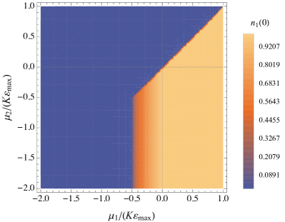
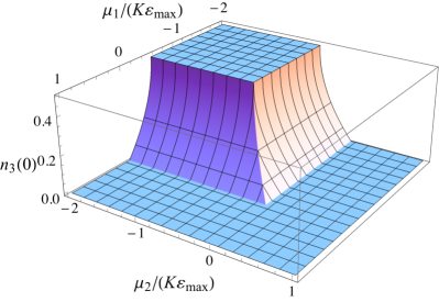
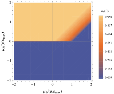
Figure 10: Contour and surface plots of the densities $n_{1}(0)$ (left) and $n_{3}(0)$ (right) for the $\mathrm{su}(2|2)$ HS chain with $\mu_{3}=0$, $K>0$ (top), and $\mu_{2}=0$, $K<0$ (bottom).

9 Conclusions

In this paper we study the thermodynamics and critical behavior of the three families of $\mathrm{su}(m|n)$ supersymmetric spin chains of Haldane–Shastry type with an additional chemical potential term. Our analysis is based on two main results, namely the computation in closed form of the partition function for an arbitrary (finite) number of spins and the derivation of a simple description of the spectrum in terms of supersymmetric motifs. By means of the transfer matrix method, we obtain an analytic expression for the free energy per site, and hence the main thermodynamic functions, in the thermodynamic limit. For the $\mathrm{su}(1|1)$, $\mathrm{su}(2|1)$ (or $\mathrm{su}(1|2)$) and $\mathrm{su}(2|2)$ chains, we identify the values of the chemical potentials for which the models are critical (gapless) by studying the low-temperature behavior of the free energy per site. In particular, we show that the central charge can take rational values that are not integers or half-integers, thus excluding the equivalence to a CFT with free bosons and/or fermions. Note, in this respect, that in order to establish the equivalence at low energies of a critical quantum system (in the thermodynamic limit) to a CFT Eq. (6.14) is necessary but not sufficient. For instance, the system’s ground state should have finite degeneracy for this equivalence to hold. Although we shall not go into specifics here, it is apparent that this condition will hold for the Hamiltonian (2.4) for generic values of the chemical potentials, since the term $H_{1}$ will break the degeneracy that the ground state of $H_{0}$ may possess (see Ref. [7] for more details). We also analyze the existence of zero-temperature phase transitions in the spin densities. More precisely, we show that in the $\mathrm{su}(1|1)$ case there are only second-order (continuous) phase transitions, while for $\mathrm{su}(2|1)$ and $\mathrm{su}(2|2)$ first-order (discontinuous) phase transitions occur in the bosonic densities when the interaction strength $K$ is positive. Moreover, for $\mathrm{su}(1|2)$ and $\mathrm{su}(2|2)$ the fermionic densities also undergo a first-order phase transition at $T=0$ for negative values of $K$.

The present work suggests several possible lines for future research. In the first place, the previous results and those of Ref. [33] seem to indicate that first-order transitions in the spin densities at $T=0$ will occur provided that $m+n>2$. It would be of interest to ascertain the validity of this conjecture, for instance by studying the behavior of these densities in the $\mathrm{su}(3)$ case. It would also be of interest to study the existence of a suitable recurrence relation for the (generalized) partition function of the models under study for arbitrary values of the chemical potentials $\mu_{\alpha}$, similar to the one derived in Ref. [29] for $\mu_{\alpha}=0$. Such a relation could then be used, by the method explained in the latter reference, to compute the central charge without explicit knowledge of the highest eigenvalue of the transfer matrix. Finally, another open problem that comes to mind is the extension of the above results to spin chains of HS type associated with root systems different than $A_{N-1}$, like $BC_{N}$, $B_{N}$ or $D_{N}$. A key step in this endeavor would be the deduction of a description of the spectrum in terms of suitable motifs. Note, in this respect, that the partition function of the supersymmetric Polychronakos–Frahm spin chain of $BC_{N}$ type with $\mu_{\alpha}=0$ is known [37], and the same is true for the ordinary (non-supersymmetric) PF chain of $D_{N}$ type [52] and the $BC_{N}$, $B_{N}$ and $D_{N}$ Haldane–Shastry chains [53, 54, 55]. However, for neither of these models an expression of the energies in terms of motifs akin to Eq. (4.9) has been found so far.

Appendix

In this Appendix we provide a justification of the different behavior of the free energy per site at finite $N$ of the $\mathrm{su}(1|1)$ chains for positive and negative values of the chemical potential $\mu$ when $K>0$ (see, e.g., Fig. 1). For simplicity, we shall restrict ourselves to the PF and FI chains (the argument for the HS chain is very similar). To begin with, for $m=n=1$ the value of $f$ at zero temperature for the PF and FI chains is given by

$$f(0)=\cases{K\varepsilon_{0}\,,&\hfill$\mu<-K\varepsilon_{\mathrm{max}}$,\hfill\cr K\int_{0}^{\mathchoice{\hbox to0.0pt{$\displaystyle{x_{0}}$\hss}}{\hbox to0.0pt{$\textstyle{x_{0}}$\hss}}{\hbox to0.0pt{$\scriptstyle{x_{0}}$\hss}}{\hbox to0.0pt{$\scriptscriptstyle{x_{0}}$\hss}}}\varepsilon(x)\,\rmd x-\mu(1-x_{0})\,,&\hfill$-K\varepsilon_{\mathrm{max}}\leqslant\mu\leqslant 0$,\hfill\cr-\mu\,,&\hfill$\mu>0$,\hfill}$$

with $K\varepsilon(x_{0})+\mu=0$ and $\varepsilon_{0}$ defined in Eq. (5.16) (cf. Section 6). On the other hand, from Eq. (4.9) for $m=n=1$ it follows that the ground state of the $\mathrm{su}(1|1)$ PF and FI chains with $K>0$ is nondegenerate for $\mu<-K\varepsilon_{\mathrm{max}}$ and $\mu>0$, since it is obtained from the unique values ${\boldsymbol{\sigma}}=(2,\dots,2)$ and ${\boldsymbol{\sigma}}=(1,\dots,1)$, respectively. The ground state energy $E_{\mathrm{GS}}$ is thus given by

$$E_{\mathrm{GS}}=\cases{J\sum_{i=1}^{N-1}{\mathcal{E}}(i)=K\sum_{i=1}^{N-1}\varepsilon(x_{i})\underset{N\to\infty}\simeq NK\varepsilon_{0}\,,&$\mu<-K\varepsilon_{\mathrm{max}}$\,,\cr-N\mu\,,&$\mu>0$.}$$

For $-K\varepsilon_{\mathrm{max}}\leqslant\mu\leqslant 0$ and large $N$, the ground state (still nondegenerate, or with very little degeneration) is instead obtained from a vector ${\boldsymbol{\sigma}}$ of the form $(2,\dots,2,1,\dots,1,2)$ with $Nx$ $2$’s and $N(1-x)$ $1$’s (where $0\leqslant x\leqslant 1$). The parameter $x$ is easily computed by minimizing the energy $E(x)$ corresponding to such a vector ${\boldsymbol{\sigma}}$, given by

$$E(x)=J\sum_{i=1}^{Nx-1}{\mathcal{E}}(i)-\mu N(1-x)\underset{N\to\infty}\simeq N\left(K\int_{0}^{x}\varepsilon(s)\,\rmd s-\mu(1-x)\right).$$

Differentiating with respect to $x$ we easily obtain $K\varepsilon(x)+\mu=0$, so that $x=x_{0}$. Thus in this case we have

$$E_{\mathrm{GS}} \simeq J\,\sum_{i=1}^{\mathchoice{\hbox to0.0pt{\hss$\displaystyle{Nx_{0}-1}$\hss}}{\hbox to0.0pt{\hss$\textstyle{Nx_{0}-1}$\hss}}{\hbox to0.0pt{\hss$\scriptstyle{Nx_{0}-1}$\hss}}{\hbox to0.0pt{\hss$\scriptscriptstyle{Nx_{0}-1}$\hss}}}{\mathcal{E}}(i)-N\mu(1-x_{0})=K\,\sum_{i=1}^{\mathchoice{\hbox to0.0pt{\hss$\displaystyle{Nx_{0}-1}$\hss}}{\hbox to0.0pt{\hss$\textstyle{Nx_{0}-1}$\hss}}{\hbox to0.0pt{\hss$\scriptstyle{Nx_{0}-1}$\hss}}{\hbox to0.0pt{\hss$\scriptscriptstyle{Nx_{0}-1}$\hss}}}\varepsilon(x_{i})-N\mu(1-x_{0})$$

$$\underset{N\to\infty}\simeq N\bigg{[}K\int_{0}^{\mathchoice{\hbox to0.0pt{$\displaystyle{x_{0}}$\hss}}{\hbox to0.0pt{$\textstyle{x_{0}}$\hss}}{\hbox to0.0pt{$\scriptstyle{x_{0}}$\hss}}{\hbox to0.0pt{$\scriptscriptstyle{x_{0}}$\hss}}}\varepsilon(x)\,\rmd x-\mu(1-x_{0})\bigg{]},\qquad-K\varepsilon_{\mathrm{max}}\leqslant\mu\leqslant 0\,.$$

In all cases, when $T\to 0$ we have ${\mathcal{Z}}\simeq\rme^{-\beta E_{\mathrm{GS}}}$, and consequently $f_{N}(0)=E_{\mathrm{GS}}/N$. From the previous expressions for the ground state energy we indeed conclude that

$$\lim_{N\to\infty}f_{N}(0)=f(0)\,,$$

as expected. However, for large though finite $N$ the value of $f_{N}(0)$ is exactly equal to $f(0)$ when $\mu\geqslant 0$, while for $\mu<0$

$$f(0)-f_{N}(0)=K\bigg{[}\int_{0}^{\mathchoice{\hbox to0.0pt{$\displaystyle{x_{0}}$\hss}}{\hbox to0.0pt{$\textstyle{x_{0}}$\hss}}{\hbox to0.0pt{$\scriptstyle{x_{0}}$\hss}}{\hbox to0.0pt{$\scriptscriptstyle{x_{0}}$\hss}}}\varepsilon(x)\,\rmd x-\frac{1}{N}\,\sum_{i=1}^{\mathchoice{\hbox to0.0pt{\hss$\displaystyle{Nx_{0}-1}$\hss}}{\hbox to0.0pt{\hss$\textstyle{Nx_{0}-1}$\hss}}{\hbox to0.0pt{\hss$\scriptstyle{Nx_{0}-1}$\hss}}{\hbox to0.0pt{\hss$\scriptscriptstyle{Nx_{0}-1}$\hss}}}\varepsilon(x_{i})\bigg{]}$$

(where $x_{0}$ should be interpreted as $1$ for $\mu<-K\varepsilon_{\mathrm{max}}$) is nonvanishing and $O(N^{-1})$.

References

References

- [1] Haldane F D M, Exact Jastrow–Gutzwiller resonating-valence-bond ground state of the spin- antiferromagnetic Heisenberg chain with exchange, 1988 Phys. Rev. Lett. 60 635
- [2] Shastry B S, Exact solution of an Heisenberg antiferromagnetic chain with long-ranged interactions, 1988 Phys. Rev. Lett. 60 639
- [3] Fowler M and Minahan J A, Invariants of the Haldane–Shastry chain, 1993 Phys. Rev. Lett. 70 2325
- [4] Bernard D, Gaudin M, Haldane F D M and Pasquier V, Yang–Baxter equation in long-range interacting systems, 1993 J. Phys. A: Math. Gen. 26 5219
- [5] Haldane F D M, Ha Z N C, Talstra J C, Bernard D and Pasquier V, Yangian symmetry of integrable quantum chains with long-range interactions and a new description of states in conformal field theory, 1992 Phys. Rev. Lett. 69 2021
- [6] Haldane F D M, “Spinon gas” description of the Heisenberg chain with inverse-square exchange: exact spectrum and thermodynamics, 1991 Phys. Rev. Lett. 66 1529
- [7] Basu-Mallick B, Bondyopadhaya N and Sen D, Low energy properties of the supersymmetric Haldane–Shastry spin chain, 2008 Nucl. Phys. B 795 596
- [8] Cirac J I and Sierra G, Infinite matrix product states, conformal field theory, and the Haldane–Shastry model, 2010 Phys. Rev. B 81 104431(4)
- [9] Greiter M and Schuricht D, No attraction between spinons in the Haldane–Shastry model, 2005 Phys. Rev. B 71 224424(4)
- [10] Greiter M, Statistical phases and momentum spacings for one-dimensional anyons, 2009 Phys. Rev. B 79 064409(5)
- [11] Finkel F and González-López A, Global properties of the spectrum of the Haldane–Shastry spin chain, 2005 Phys. Rev. B 72 174411(6)
- [12] Barba J C, Finkel F, González-López A and Rodríguez M A, The Berry–Tabor conjecture for spin chains of Haldane–Shastry type, 2008 Europhys. Lett. 83 27005(6)
- [13] Barba J C, Finkel F, González-López A and Rodríguez M A, Inozemtsev’s hyperbolic spin model and its related spin chain, 2010 Nucl. Phys. B 839 499
- [14] Enciso A, Finkel F and González-López A, Spin chains of Haldane–Shastry type and a generalized central limit theorem, 2009 Phys. Rev. E 79 060105(4)
- [15] Enciso A, Finkel F and González-López A, Level density of spin chains of Haldane–Shastry type, 2010 Phys. Rev. E 82 051117(6)
- [16] Giuliano D, Sindona A, Falcone G, Plastina F and Amico L, Entanglement in a spin system with inverse square statistical interaction, 2010 New J. Phys. 12 025022(15)
- [17] Hung C L, González-Tudela A, Cirac J I and Kimble H J, Quantum spin dynamics with pairwise-tunable, long-range interactions, 2016 Proc. Natl. Acad. Sci. U. S. A. 113 E4946
- [18] Ha Z N C and Haldane F D M, Models with inverse-square exchange, 1992 Phys. Rev. B 46 9359
- [19] Polychronakos A P, Exact spectrum of spin chain with inverse-square exchange, 1994 Nucl. Phys. B 419 553
- [20] Minahan J A and Polychronakos A P, Integrable systems for particles with internal degrees of freedom, 1993 Phys. Lett. B 302 265
- [21] Inozemtsev V I, Exactly solvable model of interacting electrons confined by the Morse potential, 1996 Phys. Scr. 53 516
- [22] Polychronakos A P, Lattice integrable systems of Haldane–Shastry type, 1993 Phys. Rev. Lett. 70 2329
- [23] Frahm H, Spectrum of a spin chain with inverse-square exchange, 1993 J. Phys. A: Math. Gen. 26 L473
- [24] Frahm H and Inozemtsev V I, New family of solvable 1D Heisenberg models, 1994 J. Phys. A: Math. Gen. 27 L801
- [25] Haldane F D M, Physics of the ideal semion gas: spinons and quantum symmetries of the integrable Haldane–Shastry spin chain, in A Okiji and N Kawakami, eds., Correlation Effects in Low-dimensional Electron Systems, Springer Series in Solid-state Sciences, volume 118, pp. 3–20
- [26] Basu-Mallick B, Ujino H and Wadati M, Exact spectrum and partition function of supersymmetric Polychronakos model, 1999 J. Phys. Soc. Jpn. 68 3219
- [27] Basu-Mallick B and Bondyopadhaya N, Exact partition functions of supersymmetric Haldane–Shastry spin chain, 2006 Nucl. Phys. B 757 280
- [28] Basu-Mallick B and Bondyopadhaya N, Spectral properties of supersymmetric Polychronakos spin chain associated with root system, 2009 Phys. Lett. A 373 2831
- [29] Hikami K and Basu-Mallick B, Supersymmetric Polychronakos spin chain: motif, distribution function, and character, 2000 Nucl. Phys. B 566 511
- [30] Basu-Mallick B, Bondyopadhaya N, Hikami K and Sen D, Boson-fermion duality in supersymmetric Haldane–Shastry spin chain, 2007 Nucl. Phys. B 782 276
- [31] Basu-Mallick B, Bondyopadhaya N and Hikami K, One-dimensional vertex models associated with a class of Yangian invariant Haldane–Shastry like spin chains, 2010 Symmetry Integr. Geom. 6 091(13)
- [32] Kuramoto Y and Yokoyama H, Exactly soluble supersymmetric --type model with long-range exchange and transfer, 1991 Phys. Rev. Lett. 67 1338
- [33] Enciso A, Finkel F and González-López A, Thermodynamics of spin chains of Haldane–Shastry type and one-dimensional vertex models, 2012 Ann. Phys.-New York 327 2627
- [34] Carrasco J A, Finkel F, González-López A, Rodríguez M A and Tempesta P, Critical behavior of supersymmetric spin chains with long-range interactions, 2016 Phys. Rev. E 93 062103(12)
- [35] Bernard D, Pasquier V and Serban D, Spinons in conformal field theory, 1994 Nucl. Phys. B 428 612
- [36] Bouwknegt P and Schoutens K, The WZW models. Spinon decomposition and yangian structure, 1996 Nucl. Phys. B 482 345
- [37] Barba J C, Finkel F, González-López A and Rodríguez M A, An exactly solvable supersymmetric spin chain of type, 2009 Nucl. Phys. B 806 684
- [38] Ahn C and Koo W M, color Calogero–Sutherland models and super Yangian algebra, 1996 Phys. Lett. B 365 105
- [39] Ahmed S, Bruschi M, Calogero F, Olshanetsky M A and Perelomov A M, Properties of the zeros of the classical polynomials and of the Bessel functions, 1979 Nuovo Cimento B 49 173
- [40] Basu-Mallick B, private communication
- [41] Mussardo G, Statistical Field Theory: an Introduction to Exactly Solved Models in Statistical Physics (Oxford: Oxford University Press) 2010
- [42] Lewin L, Polylogarithms and associated functions (New York: North Holland) 1981
- [43] Olver F W J, Lozier D W, Boisvert R F and Clark C W, eds., NIST Handbook of Mathematical Functions (Cambridge University Press) 2010
- [44] Blöte H W J, Cardy J L and Nightingale M P, Conformal invariance, the central charge, and universal finite-size amplitudes at criticality, 1986 Phys. Rev. Lett. 56 742
- [45] Affleck I, Universal term in the free energy at a critical point and the conformal anomaly, 1986 Phys. Rev. Lett. 56 746
- [46] Carrasco J A, Finkel F, González-López A and Rodríguez M A, Supersymmetric spin chains with nonmonotonic dispersion relation: Criticality and entanglement entropy, 2017 Phys. Rev. E 95 012129(15)
- [47] Kawakami N, Asymptotic Bethe-ansatz solution of multicomponent quantum systems with long-range interaction, 1992 Phys. Rev. B 46 1005
- [48] Arikawa M and Saiga Y, Exact spin dynamics of the supersymmetric - model in a magnetic field, 2006 J. Phys. A: Math. Gen. 39 10603
- [49] Potts R B, Some generalized order-disorder transformations, 1952 Math. Proc. Cambridge 48 106
- [50] Baxter R J, Exactly Solved Models in Statistical Mechanics (London: Academic Press) 1982
- [51] di Francesco P, Mathieu P and Sénéchal D, Conformal Field Theory (New York: Springer), corrected edition 1999
- [52] Basu-Mallick B, Finkel F and González-López A, Exactly solvable -type quantum spin models with long-range interaction, 2009 Nucl. Phys. B 812 402
- [53] Enciso A, Finkel F, González-López A and Rodríguez M A, Haldane–Shastry spin chains of type, 2005 Nucl. Phys. B 707 553
- [54] Basu-Mallick B, Finkel F and González-López A, The exactly solvable spin Sutherland model of type and its related spin chain, 2013 Nucl. Phys. B 866 391
- [55] Basu-Mallick B, Finkel F and González-López A, The spin Sutherland model of type and its associated spin chain, 2011 Nucl. Phys. B 843 505