Optimal measurements for quantum spatial superresolution

Abstract

We construct optimal measurements, achieving the ultimate precision predicted by quantum theory, for the simultaneous estimation of centroid, separation, and relative intensities of two incoherent point sources using a linear optical system. We discuss the physical feasibility of the scheme, which could pave the way for future practical implementations of quantum inspired imaging.

I Introduction

Metrology is the science of devising schemes that extract as precise as possible an estimate of the parameters associated with a system. The quantum foundations of this field were laid years ago Helstrom (1976); Holevo (2003); since then, most of the efforts have been devoted to single-parameter estimation, with a special emphasis in the prominent example of phase Giovannetti et al. (2011); Demkowicz-Dobrzanski et al. (2015). The quantum Cramér-Rao lower bound (qCRLB) then provides a saturable bound on the estimation uncertainty and recipes for finding the optimal measurement attaining that limit are known Braunstein and Caves (1994).

The case of multiparameter estimation is considerably more involved Yuen and Lax (1973); Belavkin (1976); Szczykulska et al. (2016). Although the equivalent qCRLB was formulated long time ago Helstrom (1967), this bound is not always saturable. The intuitive reason for this is the incompatibility of the measurements for different parameters. The conditions under which the qCRLB can be saturated have been determined Matsumoto (2002); Gill and Guta (2013) The associated optimal measurements have been worked out for pure states Pezzè et al. (2017), but for mixed states the results are fragmentary Yue et al. (2014); Zuppardo et al. (2015); Proctor et al. (2018).

In this work we will address these problems in the context of the two-point resolution limit for an optical system. In classical optics several criteria exist den Dekker and van den Bos (1997); Hemmer and Zapata (2012); Cremer and Masters (2013) to quantitatively determine these limits, the most famous of which is due to Rayleigh Rayleigh (1879).

Most of these criteria exploit properties of the point spread function (PSF) that specifies the intensity response to a point light source. This provides an intuitive picture of the mechanisms limiting resolution, but also has several shortcomings. These mainly stem from the fact that these criteria were developed for the human eye as the main detector. For example, the Rayleigh limit is defined as the distance from the center to the first minimum of the PSF, which can be made arbitrarily small with ordinary linear optics, although at the expense of the side lobes becoming much higher than the central maximum Schermelleh et al. (2010). This confirms that determining the position of the two points becomes also a question of photon statistics rather than being solely described by the Rayleigh limit.

A careful reconsideration of this conundrum has been performed in the framework of quantum estimation theory Tsang et al. (2016); Nair and Tsang (2016); Ang et al. (2016); Lupo and Pirandola (2016); Rehacek et al. (2017a); Kerviche et al. (2017); Tsang (2018); Zhou and Jiang (2018). This work showed that, in the case of two identical incoherent point sources with a priori knowledge of their centroid, the precision of an optimal measurement stays constant at all separations. As a consequence, the Rayleigh limit is subsidiary to the problem and arises because standard direct imaging discards all the phase information contained in the field. These predictions fuelled a number of proof-of-principle experiments Paur et al. (2016); Yang et al. (2016); Tham et al. (2016); Yang et al. (2017).

While remarkable, this result does not hold in the more general case of two unequally bright sources. In a suitable multiparameter scenario Chrostowski et al. (2017), where simultaneous estimation of centroid, separation, and relative brightness was considered, it was found that their estimation precisions decreased with separation Rehacek et al. (2017b). Nonetheless, an appropriate strategy was shown to lead to a significant improvement in precision at small separations over direct imaging for any fixed number of photons. The measurements attaining the ultimate quantum limits for this case are relevant to a number of applications, for example observational astronomy and microscopy.

II Model and associated multiparameter quantum Cramér-Rao bound

To be as self-contained as possible, we first set the stage for our analysis. We assume a linear spatially invariant system illuminated with quasimonochromatic paraxial waves with one specified polarization. We consider one spatial dimension; $x$ denoting the image-plane coordinate.

We phrase what follows in a quantum language that will simplify the following calculations. To a field of complex amplitude $U(x)$ we assign a ket $|U\rangle$, such that $U(x)=\langle x|U\rangle$, $|{x}\rangle$ being a point-like source at ${x}$. The system PSF is denoted by $I(x)=|\langle x|\Psi\rangle|^{2}=|\Psi(x)|^{2}$, so that $\Psi(x)$ can be interpreted as the amplitude PSF.

Two point sources, of different intensities and separated by a distance $\mathfrak{s}$, are imaged by that system. Since they are incoherent with respect to each other, the total signal must be depicted as a density operator

$$\varrho_{\bm{\theta}}=\mathfrak{q}\,\varrho_{+}+(1-\mathfrak{q})\,\varrho_{-}\,,$$ (1)

where $\mathfrak{q}$ and $1-\mathfrak{q}$ are the intensities of the sources (the total intensity is normalized to unity). The individual components $\varrho_{\pm}=|\Psi_{\pm}\rangle\langle\Psi_{\pm}|$ are just $x$-displaced PSF states; that is, $\langle x|\Psi_{\pm}\rangle=\langle x-\mathfrak{s}_{0}\mp\mathfrak{s}/2|\Psi\rangle$, so that they are symmetrically located around the geometric centroid $\mathfrak{s}_{0}$. Note that

$$|\Psi_{\pm}\rangle=\exp[-i(\mathfrak{s}_{0}\pm\mathfrak{s}/2)P]|\Psi\rangle\ ,$$ (2)

where $P$ is the momentum operator, which generates displacements in the $x$ variable, and acts as a derivative $P\mapsto-i\partial_{x}$.

The measured density matrix depends on the centroid $\mathfrak{s}_{0}$, the separation $\mathfrak{s}$, and the relative intensities of the sources $\mathfrak{q}$. This is indicated by the vector $\bm{\theta}=(\mathfrak{s}_{0},\mathfrak{s},\mathfrak{q})^{t}$. Our task is to estimate the values of $\bm{\theta}$ through the measurement of some observables on $\varrho_{\bm{\theta}}$.

In this multiparameter estimation scenario, the central quantity is the quantum Fisher information matrix (qFIM) Petz and Ghinea (2011). This is a natural generalization of the classical Fisher information, which is a mathematical measure of the sensitivity of a quantity to changes in its underlying parameters. However, the qFIM is optimized over all the possible measurements. It is defined as

$$Q_{\alpha\beta}(\bm{\theta})=\frac{1}{2}\mathrm{Tr}(\varrho_{\bm{\theta}}\{L_{\alpha},L_{\beta}\})\,,$$ (3)

where the Greek indices run over the components of the vector $\bm{\theta}$ and $\{\cdot,\cdot\}$ denotes the anticommutator. Here, $L_{\alpha}$ stands for the symmetric logarithmic derivative (SLD) Helstrom (1967) with respect the parameter $\theta_{\alpha}$:

$$\frac{1}{2}(L_{\alpha}\varrho_{\bm{\theta}}+\varrho_{\bm{\theta}}L_{\alpha})=\partial_{\alpha}\varrho_{\bm{\theta}}\,,$$ (4)

with $\partial_{\alpha}=\partial/\partial\theta_{\alpha}$.

The qFIM is a distinguishability metric on the space of quantum states and leads to the multiparameter qCRLB Braunstein and Caves (1994); Szczykulska et al. (2016) for a single detection event:

$$\mathrm{Cov}(\widehat{\bm{\theta}})\geq Q^{-1}(\bm{\theta})\,,$$ (5)

where $\mathrm{Cov}(\widehat{\bm{\theta}})$ is the covariance matrix for a locally unbiased estimator $\widehat{\bm{\theta}}$ of the quantity $\bm{\theta}$. Its matrix elements are $\mathrm{Cov}_{\alpha\beta}(\widehat{\bm{\theta}})=\mathbb{E}[(\widehat{\theta}_{\alpha}-\theta_{\alpha})(\widehat{\theta}_{\beta}-\theta_{\beta})]$, $\mathbb{E}[Y]$ being the expectation value of the random variable $Y$. The above inequality should be understood as a matrix inequality. In general, we can write $\mathrm{Tr}[\mathcal{C}\,\mathrm{Cov}(\widehat{\bm{\theta}})]\geq\mathrm{Tr}[\mathcal{C}\,Q^{-1}(\bm{\theta})]$, where $\mathcal{C}$ is some positive cost matrix, which allows us to asymmetrically prioritise the uncertainty cost of different parameters.

Unlike for a single parameter, the collective bound in (5) is not always saturable, as the measurements for different parameters may be incompatible Holevo (2003). The multiparameter qCRLB can be saturated provided

$$\mathrm{Tr}(\varrho_{\bm{\theta}}[L_{\alpha},L_{\beta}])=0\,,$$ (6)

where $[\cdot,\cdot]$ is the commutator. This condition is necessary and sufficient for pure states Matsumoto (2002); Gill and Guta (2013), upon which the criterion is equivalent to the existence of some pair of SLDs that commute. It is then possible to find an optimal measurement as the common eigenbasis of these SLDs. For mixed states, this criterion has been discussed by a number of authors Suzuki (2016) and has met some small inconsistencies in its usage, being variously identified as sufficient Vaneph et al. (2013) or necessary and sufficient Crowley et al. (2014). Reference Ragy et al. (2016) offers a clear account of this question. For our particular case, (6) is fulfilled whenever the PSF amplitude is real Rehacek et al. (2017b), $\Psi(x)^{\ast}=\Psi(x)$, which will be assumed henceforth ensuring that the parameters are therefore compatible.

For the model we are considering, and after a lengthy calculation Rehacek et al. (2017b), we obtain a compact expression for the qFIM; viz

$$Q=4\left(\begin{array}[]{ccc}p^{2}+4\mathfrak{q}(1-\mathfrak{q})\wp^{2}&(\mathfrak{q}-1/2)p^{2}&-iw\wp\\ (\mathfrak{q}-1/2)p^{2}&p^{2}/4&0\\ -iw\wp&0&\displaystyle\frac{1-w^{2}}{4\mathfrak{q}(1-\mathfrak{q})}\end{array}\right)\,,$$ (7)

which depends solely on the quantities

$$w \equiv \langle\Psi_{\pm}|\Psi_{\mp}\rangle=\langle\Psi|\exp(i\mathfrak{s}P)|\Psi\rangle\,,$$

$$p^{2} \equiv \langle\Psi_{\pm}|P^{2}|\Psi_{\pm}\rangle=\langle\Psi|P^{2}|\Psi\rangle\,,$$ (8)

$$\wp \equiv \pm\langle\Psi_{\pm}|P|\Psi_{\mp}\rangle=\langle\Psi|\exp(i\mathfrak{s}P)P|\Psi\rangle\,.$$

The quantity $p^{2}$ is determined by the shape of the PSF, whereas both $w$ and $\wp$ (which is purely imaginary) depend on the separation $\mathfrak{s}$.

Only for equally bright sources, $\mathfrak{q}=1/2$, the measurement of $\mathfrak{s}$ is uncorrelated with the other parameters. In general, when $\mathfrak{q}\neq 1/2$ the separation is correlated with the centroid (via the intensity term $\mathfrak{q}-1/2$) and the centroid is correlated with the intensity (via $p^{2}$).

The individual parameter $\theta_{\alpha}$ can be estimated with a variance satisfying $\mathrm{Var}(\widehat{\theta}_{\alpha})\geq(Q^{-1})_{\alpha\alpha}(\bm{\theta})$. It is convenient to use the inverses of the variances ${H}_{\alpha}=1/\mathrm{Var}(\theta_{\alpha})$, usually called the precisions Bernardo and Smith (2000). By inverting the QFIM and taking the limit $\mathfrak{s}\rightarrow 0$, they turn out to be Rehacek et al. (2017b)

$$H_{\mathfrak{s}_{0}}^{Q} \simeq \mathcal{Q}^{2}\,G_{22}\,\mathfrak{s}^{2}+O(\mathfrak{s}^{4})\,,$$

$$H_{\mathfrak{s}}^{Q} \simeq \frac{\mathcal{Q}^{2}}{4(1-\mathcal{Q}^{2})}\,G_{22}\,\mathfrak{s}^{2}+O(\mathfrak{s}^{4})\,,$$ (9)

$$H_{\mathfrak{q}}^{Q} \simeq \frac{1}{\mathcal{Q}^{2}}G_{22}\,\mathfrak{s}^{4}+O(\mathfrak{s}^{6})\,,$$

where

$$\mathcal{Q}^{2} = 4\mathfrak{q}(1-\mathfrak{q})<1\,,$$

$$G_{22}^{2} = \mathrm{Var}(P^{2})=\langle\Psi|P^{4}|\Psi\rangle-\langle\Psi|P^{2}|\Psi\rangle^{2}\,.$$

The superscript $Q$ indicates that the quantities are evaluated from the quantum matrix $Q$.

III Optimal measurements

We shall focus on finding measurements attaining the quantum limit, thus offering significant advantages with respect to conventional direct intensity measurements. In the general case of unequally bright sources ($\mathfrak{q}\neq 1/2$), the lack of symmetry makes this issue challenging and one cannot expect to find closed-form expressions for the optimal positive operator valued measures (POVMs) for all the values of the source parameters. However, this becomes viable when separations get very small. As already discussed, this is the most interesting regime, where conventional imaging techniques fail.

We start by specifying a basis in the signal space. A suitable choice is the set $\{|\Psi_{n}\rangle\}$ defined in terms of the spatial derivatives of the amplitude PSF:

$$\langle x|\Psi_{n}\rangle=\frac{\partial^{n}}{\partial x^{n}}\Psi(x-x_{0}),\quad n=0,1,2,\ldots,$$ (11)

where $x_{0}$ is an arbitrary displacement in the $x$-representation. We convert this set into an orthonormal basis $\{|\Phi_{n}\rangle\}$ by the standard Gram-Schmidt process. In this basis, all results can be expressed in a PSF-independent form. Moreover, signals well centered on the origin and with small separation, are represented by low-dimensional states; i.e., $\varrho_{\bm{\theta}}\rightarrow|\Phi_{0}\rangle\langle\Phi_{0}|$ for $\mathfrak{s}_{0}\rightarrow x_{0}$, and $\mathfrak{s}\rightarrow 0$.

To estimate three independent parameters, the required POVM must have at least four elements. We therefore consider the following class of measurements $\Pi_{j}=|\pi_{j}\rangle\langle\pi_{j}|$, $j=0,\ldots,2$ and $\Pi_{3}=\openone-\Pi_{0}-\Pi_{1}-\Pi_{2}$, so only three of these are independent. The first three POVM elements are defined in a four-dimensional subspace, with basis $\{|\Phi_{0}\rangle,\ldots,|\Phi_{3}\rangle\}$, wherein we expand $|\pi_{j}\rangle$ ($j=0,\ldots,2$) as

$$|\pi_{j}\rangle=\sum_{k=0}^{3}C_{jk}|\Phi_{k}\rangle\,.$$ (12)

Obviously, the projectors $|\pi_{j}\rangle\langle\pi_{j}|$ must be linearly independent. In addition, we impose the following set of conditions

$$\begin{array}[]{lcc}&|\Phi_{0}\rangle&|\Phi_{1}\rangle\\ &&\\ |\pi_{0}\rangle&C_{00}=0&C_{01}\neq 0\\ |\pi_{1}\rangle&C_{10}=0&C_{11}\neq 0\\ |\pi_{2}\rangle&C_{20}\neq 0&C_{21}\neq 0\,,\end{array}$$ (13)

where the row index can be permuted. In this way, two of the three rank-one projectors are orthogonal to the signal PSF $\Phi_{0}$; a crucial factor boosting the performance of the measurement. We stress that, by changing the displacement $x_{0}$, the basis and the measurement itself is displaced.

Next, we expand the signal components in the small parameter. We define $a_{\pm}=\mathfrak{s}_{0}\pm\mathfrak{s}-x_{0}$, so we have $\langle x|\Psi_{\pm}\rangle=\Psi(x-x_{0}-a_{\pm})$, and the expansion in $a_{\pm}$ gives

$$\langle x|\Psi_{\pm}\rangle = \sum_{m}\frac{(-a_{\pm})^{m}}{m!}\frac{\partial^{m}}{\partial x^{m}}\Psi(x-x_{0})=\sum_{m}\frac{(-a_{\pm})^{m}}{m!}\langle x|\Psi_{m}\rangle$$ (14)

$$= \langle x|\sum_{n}|\Phi_{n}\rangle\sum_{m}\frac{(-a_{\pm})^{m}}{m!}G_{nm}\,,$$

where $G_{nm}=\langle\Phi_{n}|\Psi_{m}\rangle$ [note that $G_{22}$ in Eq. (II) is consistent with this general definition]. Keeping terms up to the fourth power, we get

$$|\Psi_{\pm}\rangle \simeq \left(G_{00}+\frac{a_{\pm}^{2}}{2}G_{02}+\frac{a_{\pm}^{4}}{24}G_{04}\right)|\Phi_{0}\rangle$$ (15)

$$+ \left(a_{\pm}G_{11}+\frac{a_{\pm}^{3}}{6}G_{13}\right)|\Phi_{1}\rangle$$

$$+ \left(\frac{a_{\pm}^{2}}{2}G_{22}+\frac{a_{\pm}^{4}}{24}G_{24}\right)|\Phi_{2}\rangle$$

$$+ \frac{a_{\pm}^{3}}{6}G_{33}|\Phi_{3}\rangle\,.$$

Notice that for real amplitude PSFs, all $G$s carrying both odd and even subscripts are zero. This follows from the fact that $\langle\Psi_{n}|\Psi_{m}\rangle=0$, and hence $\langle\Psi|P^{m+n}|\Psi\rangle=0$ for any combination of odd and even subscripts, whenever the wave-function is real. We also have $G_{nm}=0$ for all $n>m$, by construction of the basis set, which makes a basis function orthogonal to all lower-order non-orthogonal functions, as the latter span a subspace that the former is orthogonal to.

We are set to evaluate the probabilities

$$p_{j}=\mathfrak{q}\langle\Psi_{+}|\Pi_{j}|\Psi_{+}\rangle+(1-\mathfrak{q})\langle\Psi_{-}|\Pi_{j}|\Psi_{-}\rangle\,,$$ (16)

and the corresponding classical Fisher information matrix per detection event:

$$F_{\alpha\beta}=\sum_{j=0}^{3}\frac{(\partial_{\alpha}p_{j})(\partial_{\beta}p_{j})}{p_{j}}\,.$$ (17)

The maximum of the classical Fisher information $F$ is its quantum version $Q$, as $Q$ is optimized over all POVMs. The corresponding precisions are thus related by $H_{\alpha}^{Q}\geq H_{\alpha}$.

Our initial strategy is to align the center of the measurement (12) with the signal centroid by letting $x_{0}=\mathfrak{s}_{0}$. The calculation of the precisions turns out to be a very lengthy task, yet the final result is surprisingly simple

$$H_{\alpha}=\lambda H_{\alpha}^{Q}\,.$$ (18)

Therefore, $H_{\alpha}$ differs from the quantum limit precision by a factor

$$\lambda=\mathcal{Q}^{2}\mathcal{A}\,,\qquad\mathcal{A}=\frac{(C_{01}C_{12}-C_{02}C_{11})^{2}}{C_{01}^{2}+C_{11}^{2}}<1\,.$$ (19)

The coefficient $\lambda$ consists of the product of two factors: one depending solely on the intensities [as defined in Eq. (II)], the other depending on the measurement. The latter one will be called the quality factor of the measurement. Conditions (13) are crucial for deriving relations (18) and (19): violating them makes the dominant terms of $H_{\alpha}$ disappear and kills the superresolution. One pertinent example would be projection on the basis set $|\Phi_{k}\rangle$: $C_{jk}=\delta_{jk}$ as for example projections on a set of Hermite-Gauss modes for a Gauss PSF advocated in Refs. Tsang et al. (2016) and Rehacek et al. (2017a) among others. Such projections can be optimal for estimating separation, but ultimately fail when separation, centroid, and intensity are to be estimated together in a multiparameter scenario considered here.

Going back to our result, two remarks are in order here. First, the performance of the measurement (12), when aligned with the centroid, scales with the same power of $\mathfrak{s}$ as the quantum limit does. The quantum limit is attained, but for a separation independent factor. This is true for all real-valued PSFs, no matter how we set the remaining free parameters of the measurement. Second, by optimizing those free parameters, the separation-independent factor $\lambda$ can be made arbitrarily close to $\lambda_{\mathrm{max}}=\mathcal{Q}^{2}$. Hence, for balanced signals ($\mathfrak{q}=1/2$), $\lambda_{\mathrm{max}}\rightarrow 1$ and the measurement (12) becomes optimal. Conversely, for unbalanced signals, the measurement is suboptimal and its performance worsens with $\mathfrak{q}$, approaching the limit $\lambda\rightarrow 0$ when $\mathfrak{q}\rightarrow 0$ and $\mathfrak{q}\rightarrow 1$.

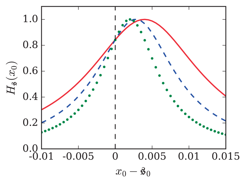
Figure 1: The precision $H_{\mathfrak{s}}$ of the separation for point objects with relative intensities $\mathfrak{q}=0.3$ and $\mathfrak{s}=0.02$ (red solid line), $\mathfrak{s}=0.014$ (blue broken line), and $\mathfrak{s}=0.01$ (green dots) as a function of misalignment $x_{0}-\mathfrak{s_{0}}$ between the measurement displacement and the centroid. The maxima of the Lorentzians are normalized to unity to make the changes in widths and centers apparent.

Next, we show that quantum limits can be saturated for any $\mathfrak{q}$ by optimizing the displacement $x_{0}$. The key point is that in the limit $\mathfrak{s}\ll 1$, the precisions $H_{\alpha}(x_{0})$, when considered as a function of the measurement displacement $x_{0}$, take a Lorentzian shape, as can be appreciated in Fig. 1 for the particular case of $H_{\mathfrak{s}}(x_{0})$. On decreasing the signal separation, the Lorentzian narrows down, with its center approaching the signal centroid. We therefore adopt the model

$$H_{\mathfrak{s}}(x_{0})=\frac{\ell_{1}\mathfrak{s}^{2}}{1+\displaystyle\frac{\ell_{2}(x_{0}-\mathfrak{s}_{0}+\ell_{3}\mathfrak{s})^{2}}{\mathfrak{s}^{2}}}\,.$$ (20)

The parameters can be identified by expanding $H_{\mathfrak{s}}$ in $\mathfrak{s}$ and $x_{0}-\mathfrak{s}_{0}$:

$$\ell_{1}\mathfrak{s}^{2}=\mathcal{A}H_{\mathfrak{s}}^{Q}\,,\quad\ell_{2}=\frac{1}{\mathfrak{q}(1-\mathfrak{q})}\,,\quad\ell_{3}=\frac{1}{2}(1-2\mathfrak{q})\,.$$ (21)

This uncovers the optimal displacement and precisions

$$x_{0}^{\mathrm{opt}}=\arg\max\limits_{x_{0}}H_{\mathfrak{s}}(x_{0})=\mathfrak{s}_{0}-\frac{1}{2}\mathfrak{s}(1-2\mathfrak{q})\,,$$

(22)

$$H_{\alpha}(x_{0}^{\mathrm{opt}})=\mathcal{A}H_{\alpha}^{Q}\,.$$

This is the central result of this paper. The optimal choice of displacement is precisely

$$x_{0}^{\mathrm{opt}}=(1-\mathfrak{q})(\mathfrak{s}_{0}-\mathfrak{s}/2)+\mathfrak{q}(\mathfrak{s}_{0}+\mathfrak{s}/2)\,,$$ (23)

so that the weighted centroid, rather than the geometrical centroid, is relevant to align the measurement. Note that the weighted centroid only coincides with the center of mass of the PSF when the PSFs are symmetric. By optimizing the measurement displacement $x_{0}$, the intensity dependent $\mathcal{Q}^{2}$ term is removed from (18) and (19) and the qCRLBs are saturated for all the signal parameters simply by letting $\mathcal{A}\rightarrow 1$. As this can be done in infinitely many ways, we conclude there are infinitely many measurements attaining the quantum limit in multiparameter superresolution imaging. They can be constructed following our recipe for any real-valued amplitude PSF.

IV Examples

To illustrate our result with a concrete example, we construct three orthogonal vectors through

$$|\pi_{\,0,1}\rangle=\left(\begin{array}[]{c}0\\ \frac{\sin(\phi/2)}{\sqrt{1+\cos\phi}}\\ \pm\frac{\cos(\phi/2)}{\sqrt{1+\cos\phi}}\\ -\sqrt{\frac{\cos\phi}{1+\cos\phi}}\end{array}\right)\,,\quad|\pi_{2}\rangle=\left(\begin{array}[]{c}\sqrt{\frac{2\cos\phi}{1+3\cos\phi}}\\ \sqrt{\frac{2\cos\phi}{1+3\cos\phi}}\\ 0\\ \sqrt{\frac{1-\cos\phi}{1+3\cos\phi}}\end{array}\right)$$ (24)

with $0<\phi<\pi/2$ in the $|\Phi_{k}\rangle$-representation, to build a family of POVMs according to the recipe (12). This measurement satisfies all the requirements, and the quality factor becomes $\mathcal{A}=1$, so that the quantum limit is attained for any real-valued PSF as long as $\mathfrak{s}\ll\sigma$.

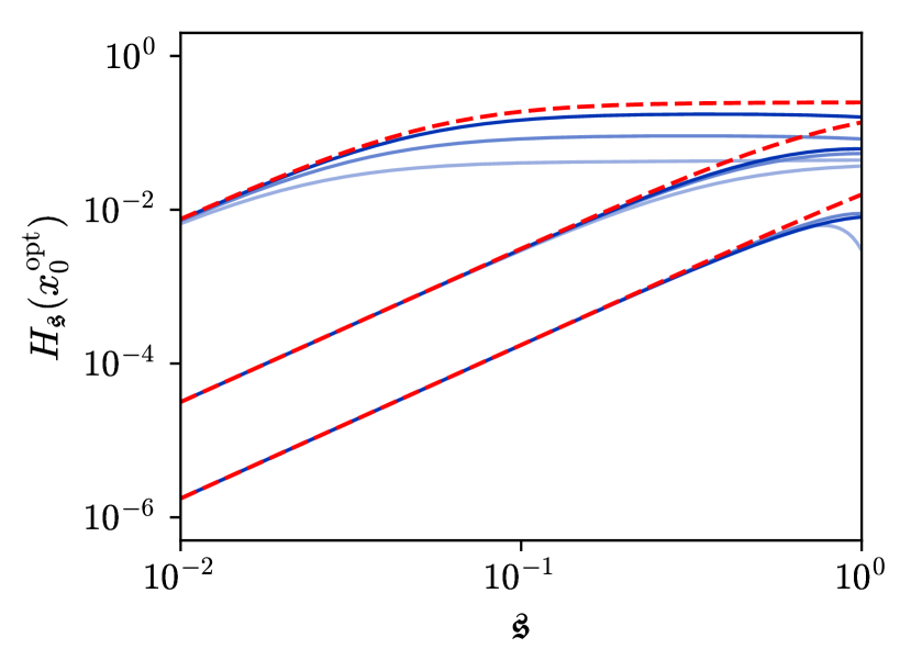
Figure 2: The precision $H_{\mathfrak{s}}(x_{0})$ for an optimally displaced measurement (24) (blue lines) as compared to the quantum limit (II) (red broken lines). The lines are grouped by the intensity difference: $\mathfrak{q}=0.49$ (top), $\mathfrak{q}=0.35$ (middle), and $\mathfrak{q}=0.1$ (bottom). Within each group (light to dark) $\phi=\pi/4$, $7\pi/20$, and $9\pi/20$, respectively. Notice the fast convergence towards the quantum limit as $\mathfrak{s}\rightarrow 0$. A Gaussian PSF of a unit width $\sigma=1$ is assumed.

The theory thus far is largely independent of the actual form of the PSF. To be more specific we adopt a Gaussian PSF, with unit width $\sigma=1$, which will serve from now on as our basis unit length. The associated orthonormal basis is then a set of displaced Hermite-Gauss modes

$$\Phi_{n}(x) = \frac{1}{(2\pi)^{\frac{1}{4}}2^{\frac{n}{2}}\sqrt{n!}}H_{n}\left((x-x_{0}^{\mathrm{opt}})/\sqrt{2}\right)$$ (25)

$$\times \exp\left[-\tfrac{1}{4}(x-x_{0}^{\mathrm{opt}})^{2}\right]\,,$$

where $H_{n}(x)$ are the Hermite polynomials. In this case, we have then $G_{22}=1/8$.

Figure 2 shows the resulting precision $H_{\mathfrak{s}}$ as a function of $\mathfrak{s}$ on a log-log scale for different intensities $\mathfrak{q}$ and different measurements of the family (24). Direct numerical evaluation of the Fisher information (17) was done using a computational basis $\{\Phi_{n}\}$ of dimension $30$ and no further approximation. With $\mathfrak{s}\rightarrow 0$ all precisions quickly converge towards the quantum limit and all the measurements (24) become optimal. Notice however that performances over a wider range of separations are sensitive to measurement parameter $\phi$ and values close to $\phi=\pi/2$ provide the best overall performance.

Having potential applications of the new detection scheme in mind we realize that achieving the quantum limits requires knowing the true values of the measured parameters. In particular, the measurement must be optimally displaced to reach the quantum limits and this displacement, through (III), depends on all the unknown signal parameters. Consequently different displacements should be used for different signals.

Can one hope to saturate the quantum limits for all signals with a fixed measurement? Unfortunately, the answer is negative. Let us consider the estimation of a signal with strongly overlapping components $\mathfrak{s}\ll 1$ of highly unequal intensities $\mathfrak{q}\rightarrow 0$ (the same analysis can be carried out for $\mathfrak{q}\rightarrow 1$), so that the weak component is outshined. To gain significant information about the weak component, the bright one must be almost completely suppressed in one of the measurement outputs. This is ensured by projecting the signal on a state that is nearly orthogonal to the bright component. That crucial projection, though, depends on both the signal centroid and separation.

Our optimal measurement also behaves in this way. Let us look at the value of $x_{0}^{\mathrm{opt}}$ in the limit $\mathfrak{q}\rightarrow 0$; i.e., when $|\Psi_{-}\rangle$ is the bright component. In this case, $x_{0}^{\mathrm{opt}}\rightarrow\mathfrak{s}_{0}-\mathfrak{s}$ coincides with the center of the bright component. But, this means that $|\Phi_{0}\rangle=|\Psi_{-}\rangle$ and the two outputs described by $|\pi_{0}\rangle$ and $|\pi_{1}\rangle$ project on subspaces orthogonal to the bright component, as anticipated.

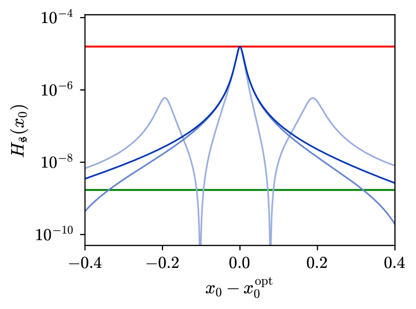
Figure 3: The precision $H_{\mathfrak{s}}$ for misaligned measurements (24) (solid blue lines) compared to the corresponding quantum (top red) and direct imaging (bottom green) limits. The parameters of the measurements are $\phi=\pi/20$ (light blue), $\pi/2$ (light blue), and $9\pi/20$ (dark blue). Observe the log vertical scale. A Gaussian PSF of a unit width $\sigma=1$ is assumed; and the sources satisfy $\mathfrak{s}=0.03$ and $\mathfrak{q}=0.1$.

In practice, the performance will be compromised by any misalignment with respect to $x_{0}^{\mathrm{opt}}$. This effect is examined in Fig. 3, where the quantum limit and the direct intensity imaging are compared with different misaligned measurements (24). Being about two orders of magnitude below the Rayleigh limit, such imperfections cause a loss of precision. Even then, the advantage with respect to direct imaging persists over a wide range of displacements $x_{0}$, demonstrating the robustness of our detection scheme. Again, setting $\phi\approx\pi/2$ seems to be the best option. For this particular example, the measurement can be misaligned by as much as $0.4\sigma$ from $x_{0}^{\mathrm{opt}}$ and still beat the direct imaging limits in measuring separations two orders of magnitude below the Rayleigh limit.

Such an inherent robustness of optimal detection schemes hints at using adaptive strategies to achieve the quantum limits. One plausible way would be to spend a portion of the photon pool to obtain a first estimate of the optimal displacement $\hat{x}_{0}^{\mathrm{opt}}=\hat{\mathfrak{s}}_{0}-\hat{\mathfrak{s}}(1-2\hat{\mathfrak{q}})/2$. Since this quantity is closely related to the weighted centroid, direct imaging can be used in this step. Then, the estimated $\hat{x}_{0}^{\mathrm{opt}}$ can be used with the optimal measurement (24) in the next step to refine the estimates of the signal parameters and so forth.

Having considered the fundamental aspects of the problem, how does one implement the optimal measurement in practice for one particular setting of the displacement? This amounts to performing simultaneous projections on three mutually orthogonal states. There exists a unitary transformation taking this triplet into another set of orthogonal vectors, where the latter set is experimentally feasible. For example the optimal projections can be mapped on three different pixels of a CCD camera. Unitary transformations of this kind can be always realized with a set of non-absorbing masks. Alternatively, giving up some performance, the implementation can be facilitated by splitting the signal beam and measuring the three projections separately. This leads to a photon loss and a threefold decrease of the precisions $H_{\alpha}$, which can be tolerated for sufficiently small separations.

V Conclusions

We have examined the ultimate limits for the simultaneous estimation of centroid, separation, and relative intensities of two incoherent point sources. Our results indicate that the optimal sub-Rayleigh resolution limit can be achieved for any real-valued amplitude PSF provided the system output is projected onto a suitable complete set of modes. Particularly useful modes can be generated from the derivatives of the system PSF, which in the limit of small separations can access all available information with a few projections.

For equally bright sources, our proposed projection is optimal whereas, for unbalanced signals, its performance deteriorates with the parameter $\mathfrak{q}$. While some of our findings were illustrated explicitly for Gaussian PSFs, our framework is general and can be applied to other relevant cases.

All in all, this constitutes an important application of multiparameter quantum estimation theory to a more realistic imaging setting. Our analysis provides a toolbox for achieving optimal resolution and paves the way for further experimental demonstrations and innovative solutions in scientific, industrial, and biomedical domains.