Limits for Rumor Spreading in stochastic populations

Biological systems can share and collectively process information to yield emergent effects, despite inherent noise in communication. While man-made systems often employ intricate structural solutions to overcome noise, the structure of many biological systems is more amorphous. It is not well understood how communication noise may affect the computational repertoire of such groups. To approach this question we consider the basic collective task of rumor spreading, in which information from few knowledgeable sources must reliably flow into the rest of the population.

In order to study the effect of communication noise on the ability of groups that lack stable structures to efficiently solve this task, we consider a noisy version of the uniform $\mathcal{PULL}$ model. We prove a lower bound which implies that, in the presence of even moderate levels of noise that affect all facets of the communication, no scheme can significantly outperform the trivial one in which agents have to wait until directly interacting with the sources. Our results thus show an exponential separation between the uniform $\mathcal{PUSH}$ and $\mathcal{PULL}$ communication models in the presence of noise. Such separation may be interpreted as suggesting that, in order to achieve efficient rumor spreading, a system must exhibit either some degree of structural stability or, alternatively, some facet of the communication which is immune to noise.

We corroborate our theoretical findings with a new analysis of experimental data regarding recruitment in Cataglyphis niger desert ants.

1 Introduction

1.1 Background and motivation

Systems composed of tiny mobile components must function under conditions of unreliability. In particular, any sharing of information is inevitability subject to communication noise. The effects of communication noise in distributed living systems appears to be highly variable. While some systems disseminate information efficiently and reliably despite communication noise [2, 22, 11, 31, 37], others generally refrain from acquiring social information, consequently losing all its potential benefits [25, 35, 38]. It is not well understood which characteristics of a distributed system are crucial in facilitating noise reduction strategies and, conversely, in which systems such strategies are bound to fail. Progress in this direction may be valuable towards better understanding the constraints that govern the evolution of cooperative biological systems.

Computation under noise has been extensively studied in the computer science community. These studies suggest that different forms of error correction (e.g., redundancy) are highly useful in maintaining reliability despite noise [3, 1, 40, 39]. All these, however, require the ability to transfer significant amount of information over stable communication channels. Similar redundancy methods may seem biologically plausible in systems that enjoy stable structures, such as brain tissues.

The impact of noise in stochastic systems with ephemeral connectivity patterns is far less understood. To study these, we focus on rumor spreading - a fundamental information dissemination task that is a prerequisite to almost any distributed system [10, 12, 16, 28]. A successful and efficient rumor spreading process is one in which a large group manages to quickly learn information initially held by one or a few informed individuals. Fast information flow to the whole group dictates that messages be relayed between individuals. Similar to the game of Chinese Whispers, this may potentially result in runaway buildup of noise and loss of any initial information [9]. It currently remains unclear what are the precise conditions that enable fast rumor spreading. On the one hand, recent works indicate that in some models of random noisy interactions, a collective coordinated process can in fact achieve fast information spreading [20, 23]. These models, however, are based on push operations that inherently include a certain reliable component (see more details in Section 1.3.2). On the other hand, other works consider computation through noisy operations, and show that several distributed tasks require significant running time [26]. The tasks considered in these works (including the problem of learning the input bits of all processors, or computing the parity of all the inputs) were motivated by computer applications, and may be less relevant for biological contexts. Moreover, they appear to be more demanding than basic tasks, such as rumor spreading, and hence it is unclear how to relate bounds on the former problems to the latter ones.

In this paper we take a general stance to identify limitations under which reliable and fast rumor spreading cannot be achieved. Modeling a well-mixed population, we consider a passive communication scheme in which information flow occurs as one agent observes the cues displayed by another. If these interactions are perfectly reliable, the population could achieve extremely fast rumor spreading [28]. In contrast, here we focus on the situation in which messages are noisy. Informally, our main theoretical result states that when all components of communication are noisy then fast rumor spreading through large populations is not feasible. In other words, our results imply that fast rumor spreading can only be achieved if either 1) the system exhibits some degree of structural stability or 2) some facet of the pairwise communication is immune to noise. In fact, our lower bounds hold even when individuals are granted unlimited computational power and even when the system can take advantage of complete synchronization.

Finally, we corroborate our theoretical findings with new analyses regarding the efficiency of information dissemination during recruitment by desert ants. More specifically, we analyze data from an experiment conducted at the Weizmann Institute of Science, concerning recruitment in Cataglyphis niger desert ants [34]. These analyses suggest that this biological system lacks reliability in all its communication components, and its deficient performances qualitatively validate our predictions. We stress that this part of the paper is highly uncommon. Indeed, using empirical biological data to validate predictions from theoretical distributed computing is extremely rare. We believe, however, that this interdisciplinary methodology may carry significant potential, and hope that this paper could be useful for future works that will follow this framework.

1.2 The problem

In this section, we give an intuitive description of the problem. Formal definitions are provided in Section 2.

Consider a population of $n$ agents. Thought of as computing entities, assume that each agent has a discrete internal state, and can execute randomized algorithms - by internally flipping coins. In addition, each agent has an opinion, which we assume for simplicity to be binary, i.e., either 0 or 1. A small number, $s$, of agents play the role of sources. Source agents are aware of their role and share the same opinion, referred to as the correct opinion. The goal of all agents is to have their opinion coincide with the correct opinion.

To achieve this goal, each agent continuously displays one of several messages taken from some finite alphabet $\Sigma$. Agents interact according to a random pattern, termed as the parallel-$\mathcal{PULL}$ model: In each round $t\in\mathbb{N}^{+}$, each agent $u$ observes the message currently displayed by another agent $v$, chosen uniformly at random (u.a.r) from all agents. Importantly, communication is noisy, hence the message observed by $u$ may differ from that displayed by $v$. The noise is characterized by a noise parameter $\delta>0$. Our model encapsulates a large family of noise distributions, making our bounds highly general. Specifically, the noise distribution can take any form, as long as it satisfies the following criterion.

Definition 1.1 (The $\delta$-uniform noise criterion).

Any time some agent $u$ observes an agent $v$ holding some message $m\in\Sigma$, the probability that $u$ actually receives a message $m^{\prime}$ is at least $\delta$, for any $m^{\prime}\in\Sigma$. All noisy samples are independent.

When messages are noiseless, it is easy to see that the number of rounds that are required to guarantee that all agents hold the correct opinion with high probability is $\mathcal{O}(\log n)$ [28]. In what follows, we aim to show that when the $\delta$-uniform noise criterion is satisfied, the number of rounds required until even one non-source agent can be moderately certain about the value of the correct opinion is very large. Specifically, thinking of $\delta$ and $s$ as constants independent of the population size $n$, this time is at least $\Omega(n)$.

To prove the lower bound, we will bestow the agents with capabilities that far surpass those that are reasonable for biological entities. These include:

• Unique identities: Agents have unique identities in the range $\{1,2,\ldots n\}$. When observing agent $v$, its identity is received without noise.

• Complete knowledge of the system: Agents have access to all parameters of the system (including $n$, $s$, and $\delta$) as well as to the full knowledge of the initial configuration except, of course, the correct opinion and the identity of the sources. In addition, agents have access to the results of random coin flips used internally by all other agents.

• Full synchronization: Agents know when the execution starts, and can count rounds.

We show that even given this extra computational power, fast convergence cannot be achieved.

1.3 Our contributions

1.3.1 Theoretical results

In all the statements that follow we consider the parallel-$\mathcal{PULL}$ model satisfying the $\delta$-uniform noise criterion, where $cs/n<\delta\leq 1/2$ for some sufficiently large constant $c$. Note that our criterion given in Definition 1.1 implies that $\delta\leq 1/|\Sigma|$. Hence, the previous lower bound on $\delta$ implies a restriction on the alphabet size, specifically, $|\Sigma|\leq n/(cs)$.

Theorem 1.2.

Any rumor spreading protocol cannot converge in less than ${\Omega}(\frac{n\delta}{s^{2}(1-2\delta)^{2}})$ rounds.

Recall that a source is aware that it is a source, but if it wishes to identify itself as such to agents that observe it, it must encode this information in a message, which is, in turn, subject to noise. We also consider the case in which an agent can reliably identify a source when it observes one (i.e.,, this information is not noisy). For this case, the following bound, which is weaker than the previous one but still polynomial, applies (a formal proof appears in Section B):

Corollary 1.3.

Assume that sources are reliably detectable. There is no rumor spreading protocol that converges in less than ${\Omega}((\frac{n\delta}{s^{2}(1-2\delta)^{2}})^{1/3})$ rounds.

Our results suggest that, in contrast to systems that enjoy stable connectivity, structureless systems are highly sensitive to communication noise. More concretely, the two crucial assumptions that make our lower bounds work are: 1) stochastic interactions, and 2) $\delta$-uniform noise (see the right column of Figure 1). When agents can stabilize their interactions the first assumption is violated. In such cases, agents can overcome noise by employing simple error-correction techniques, e.g., using redundant messaging or waiting for acknowledgment before proceeding. As demonstrated in Figure 1 (left column), when the noise is not uniform, it might be possible to overcome it with simple techniques based on using default neutral messages, and employing exceptional distinguishable signals only when necessary.

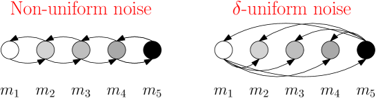
Figure 1: Non-uniform noise vs. uniform noise. On the left, we consider an example with non-uniform noise. Assume that the message vocabulary consists of 5 symbols, that is, $\Sigma=\{m_{1},m_{2},m_{3},m_{4},m_{5}\}$, where $m_{1}=0$ and $m_{5}=1$, represent the opinions. Assume that noise can occur only between consecutive messages. For example, $m_{2}$ can be observed as either $m_{2}$, $m_{3}$ or $m_{1}$, all with positive constant probability, but can never be viewed as $m_{4}$ or $m_{5}$. In this scenario, the population can quickly converge on the correct opinion by executing the following. The sources always display the correct opinion, i.e., either $m_{1}$ or $m_{5}$, and each other agent displays $m_{3}$ unless it has seen either $m_{1}$ or $m_{5}$ in which case it adopts the opinion it saw and displays it. In other words, $m_{3}$ serves as a default message for non-source agents, and $m_{1}$ and $m_{5}$ serve as attracting sinks. It is easy to see that the correct opinion will propagate quickly through the system without disturbance, and within $\mathcal{O}(\log n)$ number of rounds, where $n$ is the size of the population, all agents will hold it with high probability. In contrast, as depicted on the right picture, if every message can be observed as any other message with some constant positive probability (for clarity, some of the arrows have been omitted from the sketch), then convergence cannot be achieved in less than $\Omega(n)$ rounds, as Theorem 1.2 dictates.

1.3.2 Exponential separation between $\mathcal{PUSH}$ and $\mathcal{PULL}$

Our lower bounds on the parallel-$\mathcal{PULL}$ model (where agents observe other agents) should be contrasted with known results in the parallel-$\mathcal{PUSH}$ model, which is the push equivalent to parallel-$\mathcal{PULL}$ model, where in each round each agent may or may not actively push a message to another agent chosen u.a.r. (see also Section 2.3). Although never proved, and although their combination is known to achieve more power than each of them separately [28], researchers often view the parallel-$\mathcal{PULL}$ and parallel-$\mathcal{PUSH}$ models as very similar on complete communication topologies. Our lower bound result, however, undermines this belief, proving that in the context of noisy communication, there is an exponential separation between the two models. Indeed, when the noise level is constant for instance, convergence (and in fact, a much stronger convergence than we consider here) can be achieved in the parallel-$\mathcal{PUSH}$ using only logarithmic number of rounds [20, 23], by a simple strategy composed of two stages. The first stage consists of providing all agents with a guess about the source’s opinion, in such a way that ensures a non-negligible bias toward the correct guess. The second stage then boosts this bias by progressively amplifying it. A crucial aspect in the first stage is that agents remain silent until a certain point in time that they start sending messages continuously, which happens after being contacted for the first time. This prevents agents from starting to spread information before they have sufficiently reliable knowledge. It further allows to control the dynamics of the information spread in a balanced manner. More specifically, marking an edge corresponding to a message received for the first time by a node, the set of marked edges forms a spanning tree of low depth, rooted at the source. The depth of such tree can be interpreted as the deterioration of the message’s reliability.

On the other hand, as shown here, in the parallel-$\mathcal{PULL}$ model, even with the synchonization assumption, rumor spreading cannot be achieved in less than a linear number of rounds. Perhaps the main reason why these two models are often considered similar is that with an extra bit in the message, a $\mathcal{PUSH}$ protocol can be approximated in the $\mathcal{PULL}$ model, by letting this bit indicate whether the agent in the $\mathcal{PUSH}$ model was aiming to push its message. However, for such a strategy to work, this extra bit has to be reliable. Yet, in the noisy $\mathcal{PULL}$ model, no bit is safe from noise, and hence, as we show, such an approximation cannot work. In this sense, the extra power that the noisy $\mathcal{PUSH}$ model gains over the noisy $\mathcal{PULL}$ model, is that the very fact that one node attempts to communicate with another is reliable. This, seemingly minor, difference carries significant consequences.

1.3.3 Generalizations

Several of the assumptions discussed earlier for the parallel-$\mathcal{PULL}$ model were made for the sake of simplicity of presentation. In fact, our results can be shown to hold under more general conditions, that include: 1) different rate for sampling a source, and 2) a more relaxed noise criterion. In addition, our theorems were stated with respect to the parallel-$\mathcal{PULL}$ model. In this model, at every round, each agent samples a single agent u.a.r. In fact, for any integer $k$, our analysis can be applied to the model in which, at every round, each agent observes $k$ agents chosen u.a.r. In this case, the lower bound would simply reduce by a factor of $k$. Our analysis can also apply to a sequential variant, in which in each time step, two agents $u$ and $v$ are chosen u.a.r from the population and $u$ observes $v$. In this case, our lower bounds would multiply by a factor of $n$, yielding, for example, a lower bound of $\Omega(n^{2})$ in the case where $\delta$ and $s$ are constants.

1.3.4 Recruitment in desert ants

Our theoretical results assert that efficient rumor spreading in large groups could not be achieved without some degree of communication reliability. An example of a biological system whose communication reliability appears to be deficient in all of its components is recruitment in Cataglyphis niger desert ants. In this species, when a forager locates an oversized food item, she returns to the nest to recruit other ants to help in its retrieval [4, 34].

We complement our theoretical findings by providing new analyses from an experiment on this system conducted at the Weizmann Institute of Science [34]. In such experimental setting, we interpret our theoretical findings as an abstraction of the interaction modes between ants. While such high-level approximation may be considered very crude, we retain that it constitutes a good trade-off between analytical tractability and experimental data.

In our experimental setup recruitment happens in the small area of the nest’s entrance chamber (Figure 2a). We find that within this confined area, the interactions between ants are nearly uniform [32], such that an ant cannot control which of her nest mates she meets next (see Figure 2b). This random meeting pattern coincides with the first main assumption of our model. Additionally, it has been shown that recruitment in Cataglyphis niger ants relies on rudimentary alerting interactions [18, 27] which are subject to high levels of noise [34]. Furthermore, the responses to a recruiting ant and to an ant that is randomly moving in the nest are extremely similar [34]. Although this may resemble a noisy push interaction scheme, ants cannot reliably distinguish an ant that attempts to transmit information from any other non-communicating individual. In our theoretical framework, the latter fact means that the structure of communication is captured by a noisy-pull scheme (see more details about $\mathcal{PUSH}$ vs. $\mathcal{PULL}$ in Section 1.3.2).

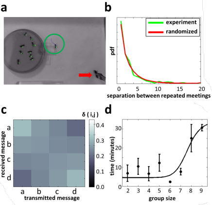
Figure 2: Unreliable communication and slow recruitment by desert ant (Cataglyphis niger). a. The experimental setup. The recruiter ant (circled) returns to the nest’s entrance chamber (dark, 9cm diameter, disc) after finding the immobilized food item (arrow). Group size is ten. b. A pdf of the number of interactions that an ant experiences before meeting the same ant twice. The pdf is compared to uniform randomized interaction pattern. Data summarizes $N=671$ interactions from seven experiments with a group size of 6 ants. c. Interactions with moving ants where classified into four different messages (’a’ to ’d’) depending on the ants’ speed. The noise at which messages were confused with each other was estimated according to the response recipient, initially stationary, ants (see Materials and Methods). Gray scale indicates the estimated overlap between every two messages $\delta(i,j)$. Note that $\delta=\min(\delta(i,j))\approx 0.2$. Data collected over $N=64$ interactions. d. The mean time it takes an ant that is informed about the food to recruit two nest-mates to exit the nest is presented for two group size ranges.

It has previously been shown that the information an ant passes in an interaction can be attributed solely to her speed before the interaction [34]. Binning ant speeds into four arbitrary discrete messages and measuring the responses of stationary ants to these messages, we can estimate the probabilities of one message to be mistakenly perceived as another one (see Materials and Methods). Indeed, we find that this communication is extremely noisy and complies with the uniform-noise assumption with a $\delta$ of approximately $0.2$ (Figure 2c).

Given the coincidence between the communication patterns in this ant system and the requirements of our lower bound we expect long delays before any uninformed ant can be relatively certain that a recruitment process is occurring. We therefore measured the time it takes an ant, that has been at the food source, to recruit the help of two nest-mates. We find that this time increases with group size ($p<0.05$ Kolmogorov-Smirnov test over $N=24$ experiments, Figure 2d). Thus, in this system, inherently noisy interactions on the microscopic level have direct implications on group level performance. While group sizes in these experiments are small, we nevertheless find these recruitment times in accordance with our asymptotic theoretical results. More details on the experimental methodology can be found in Appendix A.

1.4 Related work

Lower bound approaches in biological contexts are still extremely rare [8, 21]. Our approach can be framed within the general endeavour of addressing problems in theoretical biology through the algorithmic perspective of theoretical computer science [14, 13].

The computational study of abstract systems composed of simple individuals that interact using highly restricted and stochastic interactions has recently been gaining considerable attention in the community of theoretical computer science. Popular models include population protocols [7], which typically consider constant size individuals that interact in pairs (using constant size messages) in random communication patterns, and the beeping model [41], which assumes a fixed network with extremely restricted communication. Our model also falls in this framework as we consider the $\mathcal{PULL}$ model [16, 28, 29] with constant size messages. So far, despite interesting works that consider different fault-tolerant contexts [5, 6], most of the progress in this framework considered noiseless scenarios.

In Rumor Spreading problems (also referred to as Broadcast) a piece of information typically held by a single designated agent is to be disseminated to the rest of the population. It is the subject of a vast literature in theoretical computer science, and more specifically in the distributed computing community, see, e.g., [10, 12, 16, 17, 20, 26, 28, 33]. While some works assume a fixed topology, the canonical setting does not assume a network. Instead agents communicate through uniform $\mathcal{PUSH}/\mathcal{PULL}$ based interactions (including the phone call model), in which agents interact in pairs with other agents independently chosen at each time step uniformly at random from all agents in the population. The success of such protocols is largely due to their inherent simplicity and fault-tolerant resilience [19, 28]. In particular, it has been shown that under the $\mathcal{PUSH}$ model, there exist efficient rumor spreading protocol that uses a single bit per message and can overcome flips in messages (noise) [20].

The line of research initiated by El-Gamal [15], also studies a broadcast problem with noisy interactions. The regime however is rather different from ours: all $n$ agents hold a bit they wish to transmit to a single receiver. This line of research culminated in the $\Omega(n\log\log n)$ lower bound on the number of messages shown in [26], matching the upper bound shown many years sooner in [24].

2 Formal description of the models

We consider a population of $n$ agents that interact stochastically and aim to converge on a particular opinion held by few knowledgable individuals. For simplicity, we assume that the set of opinions contain two opinions only, namely, 0 and 1.

As detailed in this section, we shall assume that agents have access to significant amount of resources, often exceeding reasonable more realistic assumptions. Since we are concerned with lower bounds, we do not loose generality from such permissive assumptions. These liberal assumptions will actually simplify our proofs. One of these assumptions is the assumption that each agent is equipped with a unique identity $id(v)$ in the range $\{1,2,\ldots,n\}$ (see more details in Section 2.4).

2.1 Initial configuration

The initial configuration is described in several layers. First, the neutral initial configuration corresponds to the initial states of the agents, before the sources and the desired opinion to converge to are set. Then, a random initialization is applied to the given neutral initial configuration, which determines the set of sources and the opinion that agents need to converge to. This will result in what we call the charged initial configuration. It can represent, for example, an external event that was identified by few agents which now need to deliver their knowledge to the rest of the population.

Neutral Initial Configuration $\mathbf{x}^{(0)}$. Each agent $v$ starts the execution with an input that contains, in addition to its identity, an initial state taken from some discrete set of states, and a binary opinion variable $\lambda_{v}\in\{0,1\}$. The neutral initial configuration $\mathbf{x}^{(0)}$ is the vector whose $i$’th index, $\mathbf{x}^{(0)}_{i}$ for $i\in[n]$, is the input of the agent with identity $i$.

Charged Initial Configuration and Correct Opinion. The charged initial configuration is determined in three stages. The first corresponds to the random selection of sources, the second to the selection of the correct opinion, and the third to a possible update of states of sources, as a result of being selected as sources with a particular opinion.

• 1st stage - Random selection of sources. Given an integer $s\leq n$, a set $S$ of size $s$ is chosen uniformly at random (u.a.r) among the agents. The agents in $S$ are called sources. Note that any agent has equal probability of being a source. We assume that each source knows it is a source, and conversely, each non-source knows it is not a source.

• 2nd stage - Random selection of correct opinion. In the main model we consider, after sources have been determined in the first stage, the sources are randomly initialized with an opinion, called the correct opinion. That is, a fair coin is flipped to determine an opinion in $\{0,1\}$ and all sources are assigned with this opinion.

• 3rd stage - Update of initial states of sources. To capture a change in behavior as a result of being selected as a source with a particular opinion, we assume that once the opinion of a source $u$ has been determined, the initial state of $u$ may change according to some distribution $f_{source-state}$ that depends on (1) its identity, (2) its opinion, and (3) the neutral configuration. Each source samples its new state independently.

2.2 Alphabet and noisy messages

Agents communicate by observing each other according to some random pattern (for details see Section 2.3). To improve communication agents may choose which content, called message, they wish to reveal to other agents that observe them. Importantly, however, such messages are subject to noise. More specifically, at any given time, each agent $v$ (including sources) displays a message $m\in\Sigma$, where $\Sigma$ is some finite alphabet. The alphabet $\Sigma$ agents use to communicate may be richer than the actual information content they seek to disseminate, namely, their opinions. This, for instance, gives them the possibility to express several levels of certainty [30]. We can safely assume that the size of $\Sigma$ is at least two, and that $\Sigma$ includes both symbols $0$ and $1$. We are mostly concerned with the case where $\Sigma$ is of constant size (i.e., independent of the number of agents), but note that our results hold for any size of the alphabet $\Sigma$, as long as the noise criterion is satisfied (see below).

$\delta$-uniform noise. When an agent $u$ observes some agent $v$, it receives a sample of the message currently held by $v$. More precisely, for any $m,m^{\prime}\in\Sigma$, let $P_{m,m^{\prime}}$ be the probability that, any time some agent $u$ observes an agent $v$ holding some message $m\in\Sigma$, $u$ actually receives message $m^{\prime}$. The probabilities $P_{m,m^{\prime}}$ define the entries of the noise-matrix $P$ [23], which does not depend on time. We hereby also emphasize that the agents’ samples are independent.

The noise in the sample is characterized by a noise parameter $0<\delta\leq 1/2$. One of the important aspects in our theorems is that they are general enough to hold assuming any distribution governing the noise, as long as it satisfies the following noise criterion.

Definition 2.1 (The noise ellipticity parameter $\delta$).

We say that the noise has ellipticity $\delta$ if $P_{m,m^{\prime}}\geq\delta$ for any $m,m^{\prime}\in\Sigma$.

Observe that the aforementioned criterion implies that $\delta\leq 1/|\Sigma|$, and that the case $\delta=1/|\Sigma|$ corresponds to messages being completely random, and the rumor spreading problem is thus unsolvable. We next define a weaker criterion, that is particularly meaningful in cases in which sources are more restricted in their message repertoire than general agents. This may be the case, for example, if sources always choose to display their opinion as their message (possibly together with some extra symbol indicating that they are sources). Formally, we define $\Sigma^{\prime}\subseteq\Sigma$ as the set of possible messages that a source can hold together with the set of messages that can be observed when viewing a source (i.e., after noise is applied). Our theorems actually apply to the following criterion, that requires that only messages in $\Sigma^{\prime}$ are attained due to noise with some sufficient probability.

Definition 2.2 (The relaxed noise ellipticity parameter $\delta$).

We say that the noise has $\Sigma^{\prime}$-relaxed ellipticity $\delta$ if $P_{m,m^{\prime}}\geq\delta$ for any $m\in\Sigma$ and $m^{\prime}\in\Sigma^{\prime}$.

2.3 Random interaction patterns

We consider several basic interaction patterns. Our main model is the parallel-$\mathcal{PULL}$ model. In this model, time is divided into rounds, where at each round $i\in\mathbb{N}^{+}$, each agent $u$ independently selects an agent $v$ (possibly $u=v$) u.a.r from the population and then $u$ observes the message held by $v$. The parallel-$\mathcal{PULL}$ model should be contrasted with the parallel-$\mathcal{PUSH}$ model, in which $u$ can choose between sending a message to the selected node $v$ or doing nothing. We shall also consider the following variants of $\mathcal{PULL}$ model.

• $\mathcal{\mbox{\em parallel}\textnormal{-}PULL}$(k). Generalizing $\mathcal{\mbox{\em parallel}\textnormal{-}PULL}$ for an integer $1\leq k\leq n$, the $\mathcal{\mbox{\em parallel}\textnormal{-}PULL}$(k) model allows agents to observe $k$ other agents in each round. That is, at each round $i\in\mathbb{N}^{+}$, each agent independently selects a set of $k$ agents (possibly including itself) u.a.r from the population and observes each of them.

• $\mathcal{\mbox{\em sequential}\textnormal{-}PULL}$. In each time step $t\in\mathbb{N}^{+}$, two agents $u$ and $v$ are selected uniformly at random (u.a.r) among the population, and agent $u$ observes $v$.

• $\mathcal{\mbox{\em broadcast}\textnormal{-}PULL}$. It each time step $t\in\mathbb{N}^{+}$ one agent is chosen u.a.r. from the population and all agents observe it, receiving the same noisy sample of its message.

Regarding the difference in time units between the models, since interactions occur in parallel in the $\mathcal{\mbox{\em parallel}\textnormal{-}PULL}$ model, one round in that model should informally be thought of as roughly $n$ time steps in the $\mathcal{\mbox{\em sequential}\textnormal{-}PULL}$ or $\mathcal{\mbox{\em broadcast}\textnormal{-}PULL}$ model.

2.4 Liberal assumptions

As mentioned, we shall assume that agents have abilities that surpass their realistic ones. These assumption not only increases the generality of our lower bounds, but also simplifies their proofs. Specifically, the following liberal assumptions are considered.

• Unique identities. Each agent is equipped with a unique identity $id(v)\in\{1,2,\ldots,n\}$, that is, for every two agents $u$ and $v$, we have $id(u)\neq id(v)$. Moreover, whenever an agent $u$ observes some agent $v$, we assume that $u$ can infer the identity of $v$. In other words, we provide agents with the ability to reliably distinguish between different agents at no cost.

• Unlimited internal computational power. We allow agents to have unlimited computational abilities including infinite memory capacity. Therefore, agents can potentially perform arbitrarily complex computations based on their knowledge (and their $id$).

• Complete knowledge of the system. Informally, we assume that agents have access to the complete description of the system except for who are the sources and what is their opinion. More formally, we assume that each agent has access to:

  • the neutral initial configuration $\mathbf{x}^{(0)}$,

  • all the systems parameters, including the number of agents $n$, the noise parameter $\delta$, the number of sources $s$, and the distribution $f_{source-state}$ governing the update the states of sources in the third stage of the charged initial configuration.

• Full synchronization. We assume that all agents are equipped with clocks that can count time steps (in $\mathcal{\mbox{\em sequential}\textnormal{-}PULL}$ or $\mathcal{\mbox{\em broadcast}\textnormal{-}PULL}$) or rounds (in $\mathcal{\mbox{\em parallel}\textnormal{-}PULL}$(k)). The clocks are synchronized, ticking at the same pace, and initialized to 0 at the beginning of the execution. This means, in particular, that if they wish, the agents can actually share a notion of time that is incremented at each time step.

• Shared randomness. We assume that algorithms can be randomized. That is, to determine the next action, agents can internally toss coins and base their decision on the outcome of these coin tosses. Being liberal, we shall assume that randomness is shared in the following sense. At the outset, an arbitrarily long sequence $r$ of random bits is generated and the very same sequence $r$ is written in each agent’s memory before the protocol execution starts. Each agent can then deterministically choose (depending on its state) which random bits in $r$ to use as the outcome of its own random bits. This implies that, for example, two agents can possibly make use of the very same random bits or merely observe the outcome of the random bits used by the other agents. Note that the above implies that, conditioning on an agent $u$ being a non-source agent, all the random bits used by $u$ during the execution are accessible to all other agents.

• Coordinated sources. Even though non-source agents do not know who the sources are, we assume that sources do know who are the other sources. This means, in particular, that the sources can coordinate their actions.

2.5 Considered algorithms and solution concept

Upon observation, each agent can alter its internal state (and in particular, its message to be seen by others) as well as its opinion. The strategy in which agents update these variables is called “algorithm”. As mentioned, algorithms can be randomized, that is, to determine the next action, agents can use the outcome of coin tosses in the sequence $r$ (see Shared randomness in Section 2.4). Overall, the action of an agent $u$ at time $t$ depends on:

1. the initial state of $u$ in the charged initial configuration (including the identity of $u$ and whether or not it is a source),

2. the initial knowledge of $u$ (including the system’s parameters and neutral configuration),

3. the time step $t$, and the list of its observations (history) up to time $t-1$, denoted $x_{u}^{(<t)}$,

4. the sequence of random bits $r$.

2.6 Convergence and time complexity

At any time, the opinion of an agent can be viewed as a binary guess function that is used to express its most knowledgeable guess of the correct opinion. The agents aim to minimize the probability that they fail to guess this opinion. In this context, it can be shown that the optimal guessing function is deterministic.

Definition 2.3.

We say that convergence has been achieved if one can specify a particular non-source agent $v$, for which is it guaranteed that its opinion is the correct opinion with probability at least $2/3$. The time complexity is the number of time steps (respectively, rounds) required to achieve convergence.

We remark that the latter definition encompasses all three models considered.

Remark 2.4 (Different sampling rates of sources).

We consider sources as agents in the population but remark that they can also be thought of as representing the environment. In this case, one may consider a different rate for sampling a source (environment) vs. sampling a typical agent. For example, the probability to observe any given source (or environment) may be $x$ times more than the probability to observe any given non-source agent. This scenario can also be captured by a slight adaptation of our analysis. When $x$ is an integer, we can alternatively obtain such a generalization by considering additional artificial sources in the system. Specifically, we replace each source $u_{i}$ with a set of sources $U_{i}$ consisting of $x$ sources that coordinate their actions and behave identically, simulating the original behavior of $u_{i}$. (Recall that we assume that sources know who are the other sources and can coordinate their actions.) Since the number of sources increases by a multiplicative factor of $x$, our lower bounds (see Theorem 3.1 and Corollary 1.3) decrease by a multiplicative factor of $x^{2}$.

3 The lower bounds

Throughout this section we consider $\delta<1/2$, such that $\frac{(1-2\delta)}{\delta sn}\leq\frac{1}{10}$. Our goal in this section is to prove the following result.

Theorem 3.1.

Assume that the relaxed $\delta$-uniform noise criterion is satisfied.

• Let $k$ be an integer. Any rumor spreading protocol on the $\mathcal{\mbox{\em parallel}\textnormal{-}PULL}$(k) model cannot converge in fewer rounds than $\Omega\left(\frac{n\delta}{ks^{2}(1-2\delta)^{2}}\right).$

• Consider either the $\mathcal{\mbox{\em sequential}\textnormal{-}PULL}$ or the $\mathcal{\mbox{\em broadcast}\textnormal{-}PULL}$ model. Any rumor spreading protocol cannot converges in fewer rounds than $\Omega\left(\frac{n^{2}\delta}{s^{2}(1-2\delta)^{2}}\right).$

To prove the theorem, we first prove (in Section 3.1) that an efficient rumor spreading algorithm in either the noisy $\mathcal{\mbox{\em sequential}\textnormal{-}PULL}$ model or the $\mathcal{\mbox{\em parallel}\textnormal{-}PULL}$(k) model can be used to construct an efficient algorithm in the $\mathcal{\mbox{\em broadcast}\textnormal{-}PULL}$ model. The resulted algorithm has the same time complexity as the original one in the context of $\mathcal{\mbox{\em sequential}\textnormal{-}PULL}$ and adds a multiplicative factor of $kn$ in the context of $\mathcal{\mbox{\em parallel}\textnormal{-}PULL}$(k).

We then show how to relate the rumor spreading problem in $\mathcal{\mbox{\em broadcast}\textnormal{-}PULL}$ to a statistical inference test (Section 3.2). A lower bound on the latter setting is then achieved by adapting techniques from mathematical statistics (Section 3.3).

3.1 Reducing to the $\mathcal{\mbox{\em broadcast}\textnormal{-}PULL}$ Model

The following lemma establishes a formal relation between the convergence times of the models we consider. We assume all models are subject to the same noise distribution.

Lemma 3.2.

Any protocol operating in $\mathcal{\mbox{\em sequential}\textnormal{-}PULL}$ can be simulated by a protocol operating in $\mathcal{\mbox{\em broadcast}\textnormal{-}PULL}$ with the same time complexity. Moreover, for any integer $1\leq k\leq n$, any protocol $\mathcal{P}$ operating in $\mathcal{\mbox{\em parallel}\textnormal{-}PULL}$(k) can be simulated by a protocol operating in $\mathcal{\mbox{\em broadcast}\textnormal{-}PULL}$ with a time complexity that is $kn$ times that of $\mathcal{P}$ in $\mathcal{\mbox{\em parallel}\textnormal{-}PULL}$(k).

Proof.

Let us first show how to simulate a time step of $\mathcal{\mbox{\em sequential}\textnormal{-}PULL}$ in the
$\mathcal{\mbox{\em broadcast}\textnormal{-}PULL}$ model. Recall that in $\mathcal{\mbox{\em broadcast}\textnormal{-}PULL}$, in each time step, all agents receive the same observation sampled u.a.r from the population. Upon drawing such an observation, all agents use their shared randomness to generate a (shared) uniform random integer $X$ between $1$ and $n$. Then, the agent whose unique identity corresponds to $X$ is the one processing the observation, while all other agents ignore it. This reduces the situation to a scenario in $\mathcal{\mbox{\em sequential}\textnormal{-}PULL}$, and the agents can safely execute the original algorithm designed for that model.

As for simulating a time step of $\mathcal{\mbox{\em parallel}\textnormal{-}PULL}$(k) in $\mathcal{\mbox{\em broadcast}\textnormal{-}PULL}$, agents divide time steps in the latter model into rounds, each composing of precisely $kn$ time steps. Recall that the model assumes that agents share clocks that start when the execution starts and tick at each time step. This implies that the agents can agree on the division of time into rounds, and can further agree on the round number. For $1\leq i\leq kn$, during the $i$-th step of each round, only the agent whose identity is ($i$ mod $n$)$+1$ receives the observation, while all other agents ignore it. This ensures that when a round is completed in the $\mathcal{\mbox{\em broadcast}\textnormal{-}PULL}$ model, each agent receives precisely $k$ independent uniform samples as it would in a round of $\mathcal{\mbox{\em parallel}\textnormal{-}PULL}$(k). Therefore, at the end of each round $j\in\mathbb{N}^{+}$ in the $\mathcal{\mbox{\em broadcast}\textnormal{-}PULL}$ model, all agents can safely execute their actions in the $j$’th round of the original protocol designed for $\mathcal{\mbox{\em parallel}\textnormal{-}PULL}$(k). This draws a precise bijection from rounds in $\mathcal{\mbox{\em parallel}\textnormal{-}PULL}$(k) and rounds in $\mathcal{\mbox{\em broadcast}\textnormal{-}PULL}$. The multiplicative overhead of $kn$ simply follows from the fact that each round in $\mathcal{\mbox{\em broadcast}\textnormal{-}PULL}$ consists of $kn$ time steps. ∎

Thanks to Lemma 3.2, Theorem 3.1 directly follows from the next theorem.

Theorem 3.3.

Consider the $\mathcal{\mbox{\em broadcast}\textnormal{-}PULL}$ model and assume that the relaxed $\delta$-uniform noise criterion is satisfied. Any rumor spreading protocol cannot converges in fewer time steps than $\Omega\left(\frac{n^{2}\delta}{s^{2}(1-2\delta)^{2}}\right)~{}.$

The remaining of the section is dedicated to proving Theorem 3.3. Towards achieving this, we view the task of guessing the correct opinion in the $\mathcal{\mbox{\em broadcast}\textnormal{-}PULL}$ model, given access to noisy samples, within the more general framework of distinguishing between two types of stochastic processes which obey some specific assumptions.

3.2 Rumor Spreading and hypothesis testing

To establish the desired lower bound, we next show how the rumor spreading problem in the broadcast-$\mathcal{PULL}$ model relates to a statistical inference test. That is, from the perspective of a given agent, the rumor spreading problem can be understood as the following: Based on a sequence of noisy observations, the agent should be able to tell whether the correct opinion is $0$ or $1$. We formulate this problem as a specific task of distinguishing between two random processes, one originated by running the protocol assuming the correct opinion is 0 and the other assuming it is 1.

One of the main difficulties lies in the stochastic dependencies affecting these processes. In general, at different time steps, they do not consist of independent draws of a given random variable. In other words, the law of an observation not only depends on the correct opinion, on the initial configuration and on the underlying randomness used by agents, but also on the previous noisy observation samples and (consequently) on the messages agents themselves choose to display on that round. An intuitive version of this problem is the task of distinguishing between two (multi-valued) biased coins, whose bias changes according to the previous outcomes of tossing them (e.g., due to wear). Following such intuition, we define the following general class of Adaptive Coin Distinguishing Tasks, for short $\tt ACDT$.

Definition 3.4 ($\tt ACDT$).

A distinguisher is presented with a sequence of observations taken from a coin of type $\eta$ where $\eta\in\{0,1\}$. The type $\eta$ is initially set to $0$ or $1$ with probability $1/2$ (independently of everything else). The goal of the distinguisher is to determine the type $\eta$, based on the observations. More specifically, for a given time step $t$, denote the sequence of previous observations (up to, and including, time $t-1$) by $x^{(<t)}=(x^{(1)},\dots,x^{(t-1)}).$ At each time $t$, given the type $\eta\in\{0,1\}$ and the history of previous observations $x^{(<t)}$, the distinguisher receives an observation $X^{(t)}_{\eta}\in\Sigma$, which has law $P(X_{\eta}^{(t)}=m\mid x^{(<t)}).$

We next introduce, for each $m\in\Sigma$, the parameter

$$\varepsilon(m,x^{(<t)})=P(X_{1}^{(t)}=m\mid x^{(<t)})-P(X_{0}^{(t)}=m\mid x^{(<t)}).$$

Since, at all times $t$, it holds that

$$\sum_{m\in\Sigma}P(X_{0}^{(t)}=m\mid x^{(<t)})=\sum_{m\in\Sigma}P(X_{1}^{(t)}=m\mid x^{(<t)})=1,$$

then $\sum_{m\in\Sigma}\varepsilon(m,x^{(<t)})=0$. We shall be interested in the quantity $d_{\varepsilon}(x^{(<t)}):=\sum_{m\in\Sigma}|\varepsilon(m,x^{(<t)})|,$ which corresponds to the $\ell_{1}$ distance between the distributions $P(X_{0}^{(t)}=m\mid x^{(<t)})$ and $P(X_{1}^{(t)}=m\mid x^{(<t)})$ given the sequence of previous observations.

Definition 3.5 (The bounded family ${\tt ACDT}(\varepsilon,\delta)$).

We consider a family of instances of $\tt ACDT$, called ${\tt ACDT}(\varepsilon,\delta)$, governed by parameters $\varepsilon$ and $\delta$. Specifically, this family contains all instances of ${\tt ACDT}$ such that for every $t$, and every history $x^{(<t)}$, we have:

• $d_{\varepsilon}(x^{(<t)})\leq\varepsilon$, and

• $\forall m\in\Sigma$ such that $\varepsilon(m,x^{(<t)})\neq 0$, we have $\delta\leq P(X_{\eta}^{(t)}=m\mid x^{(<t)})$ for $\eta\in\left\{0,1\right\}$.

In the rest of the current section, we show how Theorem 3.3, that deals with the $\mathcal{\mbox{\em broadcast}\textnormal{-}PULL}$ model, follows directly from the next theorem that concerns the adaptive coin distinguishing task, by setting $\varepsilon=\frac{2s(1-2\delta)}{n}.$ The actual proof of Theorem 3.6 appears in Section 3.3.

Theorem 3.6.

Consider any protocol for any instance of $\tt ACDT(\varepsilon,\delta)$, The number of samples required to distinguish between a process of type $0$ and a process of type $1$ with probability of error less than $\frac{1}{3}$ is at least $\frac{\ln 2}{9}\left(\frac{6(\delta-\varepsilon)^{3}}{\delta^{3}-\delta^{2}\varepsilon+3\delta\varepsilon^{2}-\varepsilon^{3}}\right)\frac{\delta}{\varepsilon^{2}}.$ In particular, if $\frac{\varepsilon}{\delta}<{10}$, then the number of necessary samples is $\Omega\left(\frac{\delta}{\varepsilon^{2}}\right)$.

3.2.1 Proof of Theorem 3.3 assuming Theorem 3.6

Consider a rumor spreading protocol $\cal{P}$ in the $\mathcal{\mbox{\em broadcast}\textnormal{-}PULL}$ model. Fix a node $u$. We first show that running $\cal{P}$ by all agents, the perspective of node $u$ corresponds to a specific instance of $\tt ACDT(\frac{2s(1-2\delta)}{n},\delta)$ called $\Pi(\mathcal{P},u)$. We break down the proof of such correspondence into two claims.

The $\tt ACDT$ instance $\Pi(\mathcal{P},u)$.

Recall that we assume that each agent knows the complete neutral initial configuration, the number of sources $s$, and the shared of random bits sequence $r$. We avoid writing such parameters as explicit arguments to $\Pi(\mathcal{P},u)$ in order to simplify notation, however, we stress that what follows assumes that these parameters are fixed. The bounds we show hold for any fixed value of $r$ and hence also when $r$ is randomized.

Each agent is interested in discriminating between two families of charged initial configurations: Those in which the correct opinion is $0$ and those in which it is $1$ (each of these possibilities occurs with probability $\frac{1}{2}$). Recall that the correct opinion is determined in the 2nd stage of the charged initial configuration, and is independent form the choice of sources (1st stage).

We next consider the perspective of a generic non-source agent $u$, and define the instance $\Pi(\mathcal{P},u)$ as follows. Given the history $x^{(<t)}$, we set $P(X_{\eta}^{(t)}=m\mid x^{(<t)})$, for $\eta\in\left\{0,1\right\}$, to be equal to the probability that $u$ observes message $m\in\Sigma$ at time step $t$ of the execution $\cal{P}$. For clarity’s sake, we remark that the latter probability is conditional on: the history of observations being $x^{(<t)}$, ,the sequence of random bits $r$, ,the correct opinion being $\eta\in\{0,1\}$, ,the neutral initial configuration, ,the identity of $u$, ,the algorithm $\mathcal{P}$, and the system’s parameters (including the distribution $f_{source-state}$ and the number of sources $s$).

Claim 3.7.

Let $\cal{P}$ be a correct protocol for the rumor spreading problem in $\mathcal{\mbox{\em broadcast}\textnormal{-}PULL}$ and let $u$ be an agent for which the protocol is guaranteed to produce the correct opinion with probability at least $p$ by some time $T$ (if one exists), for any fixed constant $p\in(0,1)$. Then $\Pi({\cal{P}},u)$ can be solved in time $T$ with correctness being guaranteed with probability at least $p$.

Proof.

Conditioning on $\eta\in\{0,1\}$ and on the random seed $r$, the distribution of observations in the $\Pi(\mathcal{P},u)$ instance follows precisely the distribution of observations as perceived from the perspective of $u$ in $\mathcal{\mbox{\em broadcast}\textnormal{-}PULL}$. Hence, if the protocol $\cal{P}$ at $u$ terminates with output $j\in\{0,1\}$ at round $T$, after the $T$-th observation in $\Pi({\cal{P}},u)$ we can set $\Pi({\cal{P}},u)$’s output to $j$ as well. Given that the two stochastic processes have the same law, the correctness guarantees are the same. ∎

Lemma 3.8.

$\Pi({{\cal{P}},u})\in\tt ACDT\left(\frac{2(1-2\delta)s}{n},\delta\right)$.

Proof.

Since the noise in $\mathcal{\mbox{\em broadcast}\textnormal{-}PULL}$ flips each message $m\in\Sigma$ into any $m^{\prime}\in\Sigma^{\prime}$ with probability at least $\delta$, regardless of the previous history and of $\eta\in\{0,1\}$, at all times $t$, if $m\in\Sigma^{\prime}$ then $P(X_{\eta}^{(t)}=m\mid x^{(<t)})\geq\delta.$ Consider a message $m\in\Sigma\setminus\Sigma^{\prime}$ (if such a message exists). By definition, such a message could only be received by observing a non-source agent. But given the same history $x^{(<t)}$, the same sequence of random bits $r$, and the same initial knowledge, the behavior of a non-source agent is the same, no matter what is the correct opinion $\eta$. Hence, for $m\in\Sigma\setminus\Sigma^{\prime}$ we have $P(X_{0}^{(t)}=m\mid x^{(<t)})=P(X_{1}^{(t)}=m\mid x^{(<t)})$, or in other words, $m\in\Sigma\setminus\Sigma^{\prime}\implies\varepsilon(m,x^{(<t)})=0.$

It remains to show that $d_{\varepsilon}(x^{(<t)})\leq\frac{2(1-2\delta)s}{n}$. Let us consider two executions of the rumor spreading protocol, with the same neutral initial configuration, same shared sequence of random bits $r$, same set of sources, except that in the first the correct opinion is $0$ while in the other it is $1$. Let us condition on the history of observations $x^{(<t)}$ being the same in both processes. As mentioned, given the same history $x^{(<t)}$, the behavior of a non-source agent is the same, regardless of the correct opinion $\eta$. It follows that the difference in the probability of observing any given message is only due to the event that a source is observed. Recall that the number of sources is $s$. Therefore, the probability of observing a source is $s/n$, and we may write as a first approximation $\varepsilon(m,x^{(<t)})\leq s/n$ . However, we can be more precise. In fact, $\varepsilon(m,x^{(<t)})$ is slightly smaller than $s/n$, because the noise can still affect the message of a source. We may interpret $\varepsilon(m,x^{(<t)})$ as the following difference. For a source $v\in S$, let $m_{\eta}^{v}$ be the message of $u$ assuming the given history $x^{(<t)}$ and that $v$ is of type $\eta\in\{0,1\}$ (the message $m_{\eta}^{v}$ is deterministically determined given the sequence $r$ of random bits, the neutral initial configuration, the parameters of the system, and the identity of $v$). Let $\alpha_{m^{\prime},m}$ be the probability that the noise transforms a message $m^{\prime}$ into a message $m$. Then $\varepsilon(m,x^{(<t)})=\frac{1}{n}\sum_{v\in S}(\alpha_{m_{1}^{v},m}-\alpha_{m_{0}^{v},m}),$ and

$$d_{\varepsilon}(x^{(<t)})=\sum_{m\in\Sigma}|\varepsilon(m,x^{(<t)})|\leq\frac{1}{n}\sum_{m\in\Sigma}\sum_{v\in S}|\alpha_{m_{1}^{v},m}-\alpha_{m_{0}^{v},m}|.$$ (1)

By the definition of ${\tt ACDT}(\varepsilon,\delta)$, it follows that either $\alpha_{m_{1}^{v},m}=\alpha_{m_{0}^{v},m}$ (if $\varepsilon(m,x^{(<t)})=0$) or $\delta\leq\alpha_{m_{1}^{v},m},\alpha_{m_{0}^{v},m}\leq 1-\delta$ (if $\varepsilon(m,x^{(<t)})\neq 0$). Thus, to bound the right hand side in (1), we can use the following claim.

Claim 3.9.

Let $P$ and $Q$ be two distributions over a universe $\Sigma$ such that for any element $m\in\Sigma$, $\delta\leq P(m),Q(m)\leq 1-\delta.$ Then $\sum_{m\in\Sigma}\lvert P(m)-Q(m)\rvert\leq 2(1-2\delta).$

Proof of Claim 3.9.

Let $\Sigma_{+}:=\{m:P(m)>Q(m)\}$. We may write

$$\sum_{m\in\Sigma}\lvert P(m)-Q(m)\rvert =\sum_{m\in\Sigma_{+}}(P(m)-Q(m))+\sum_{m\in setminus\Sigma_{+}}(Q(m)-P(m))$$

$$=P(\Sigma_{+})-Q(\Sigma_{+})+Q(\Sigma\setminus\Sigma_{+})-P(\Sigma\setminus\Sigma_{+})$$

$$=2(P(\Sigma_{+})-Q(\Sigma_{+})),$$

where in the last line we used the fact that $Q(\Sigma\setminus\Sigma_{+})-P(\Sigma\setminus\Sigma_{+})=1-Q(\Sigma_{+})-1+P(\Sigma_{+})=P(\Sigma_{+})-Q(\Sigma_{+}).$ We now distinguish two cases. Case $1$.If $\Sigma_{+}$ is a singleton, $\Sigma_{+}=\{m^{*}\}$, then $P(\Sigma_{+})-Q(\Sigma_{+})=P(m^{*})-Q(m^{*})\leq 1-2\delta$, by assumption. Case $2$. Otherwise, $\lvert\Sigma_{+}\rvert\geq 2$ and $2\sum_{m\in\Sigma_{+}}(P(m)-Q(m))\leq 2-2\sum_{m\in\Sigma_{+}}Q(m)\leq 2(1-\delta\lvert\Sigma_{+}\rvert)\leq 2(1-2\delta)$, using the fact that for any $m$, $Q(m)\geq\delta$, and the fact that $P$ is a probability measure. This completes the proof of Claim 3.9. ∎

Applying Claim 3.9 for a fixed $v\in S$ to distributions $(\alpha_{m_{0}^{v},m})_{m}$ and $(\alpha_{m_{1}^{v},m})_{m}$, we obtain

$$\frac{1}{n}\sum_{m\in\Sigma}\sum_{v\in S}|\alpha_{m_{1}^{v},m}-\alpha_{m_{0}^{v},m}|\leq\frac{1}{n}2\sum_{v\in S}(1-2\delta)\leq\frac{2(1-2\delta)s}{n}.$$

Hence, we have $\Pi({\cal{P}})\in\tt ACDT\left(\frac{2(1-2\delta)s}{n},\delta\right)$, establishing Lemma 3.8. ∎

Thanks to Claims 3.7 and Lemma 3.8, Theorem 3.3 regarding the $\mathcal{\mbox{\em broadcast}\textnormal{-}PULL}$ model becomes a direct consequence of Theorem 3.6 on the adaptive coin distinguishing task, taking $\varepsilon=\frac{2(1-2\delta)s}{n}~{}.$ More precisely, the assumption $\frac{(1-2\delta)}{\delta sn}\leq c$ for some small constant $c$, ensures that $\frac{\varepsilon}{\delta}\leq c$ as required by Theorem 3.6. The lower bound $\Omega\left(\frac{\varepsilon^{2}}{\delta}\right)$ corresponds to $\Omega\left(\frac{n^{2}\delta}{(1-2\delta)^{2}s^{2}}\right)~{}.$ This concludes the proof of Theorem 3.3. ∎

To establish our results it remains to prove Theorem 3.6.

3.3 Proof of Theorem 3.6

We start by recalling some facts from Hypothesis Testing. First let us recall two standard notions of (pseudo) distances between probability distributions. Given two discrete distributions $P_{0},P_{1}$ over a probability space $\Omega$ with the same support, the total variation distance is defined as $TV(P_{0},P_{1}):=\frac{1}{2}\sum_{x\in\Omega}\lvert P_{0}(x)-P_{1}(x)\rvert,$ and the Kullback-Leibler divergence $KL(P_{0},P_{1})$ is defined as $KL(P_{0},P_{1}):=\sum_{x\in\Omega}P_{0}(x)\log\frac{P_{1}(x)}{P_{0}(x)}.$

The following lemma shows that, when trying to discriminate between distributions $P_{0},P_{1}$, the total variation relates to the smallest error probability we can hope for.

Lemma 3.10 (Neyman-Pearson [36, Lemma $5.3$ and Proposition $5.4$]).

Let $P_{0},P_{1}$ be two distributions. Let $X$ be a random variable of law either $P_{0}$ or $P_{1}$. Consider a (possibly probabilistic) mapping $f:\Omega\rightarrow\{0,1\}$ that attempts to “guess” whether the observation $X$ was drawn from $P_{0}$ (in which case it outputs $0$) or from $P_{1}$ (in which case it outputs $1$). Then, we have the following lower bound,

$$\text{${\textstyle P_{0}}$}\left(f(X)=1\right)+\text{${\textstyle P_{1}}$}\left(f(X)=0\right)\geq 1-TV(P_{0},P_{1}).$$ (2)

The total variation is related to the $KL$ divergence by the following inequality.

Lemma 3.11 (Pinsker [36, Lemma $5.8$]).

For any two distributions $P_{0},P_{1}$,

$$TV(P_{0},P_{1})\leq\sqrt{KL\left(P_{0},P_{1}\right)}.$$ (3)

We are now ready to prove the theorem.

Proof of Theorem 3.6.

Let us define $\text{${\textstyle P_{\eta}}$}\left(\ \cdot\ \right)=P\left(\ \cdot\ |\ \text{``correct distribution is $\eta$''}\right)$ for $\eta\in\left\{0,1\right\}$. We denote $P^{(\leq t)}_{\eta}$, $\eta\in\left\{0,1\right\}$, the two possible distributions of $\mathbf{X}^{(\leq t)}$. We refer to $P_{0}^{(\leq t)}$ as the distribution of type $0$ and to $P_{1}^{(\leq t)}$ as the distribution of type $1$. Furthermore, we define the correct type of a sequence of observations $\mathbf{X}^{(\leq t)}$ to be $0$ if the observations are sampled from $P^{(\leq t)}_{0}$, and to be $1$ if they are sampled from $P^{(\leq t)}_{1}$.

After $t$ observations $\mathbf{x}^{(\leq t)}=(x^{(1)},\dots,x^{(t)})$ we have to decide whether the distribution is of type $0$ or $1$. Our goal is to maximize the probability of guessing the type of the distribution, observing $\mathbf{X}^{(\leq t)}$, which means that we want to minimize

$$f=\sum_{\eta\in\{0,1\}}P_{\eta}\left(f(\mathbf{X}^{(\leq t)})=1-\eta\right)P\left(\text{``correct type is $\eta$''}\right).$$ (4)

Recall that the correct type is either $0$ or $1$ with probability $\frac{1}{2}$. Thus, the error probability described in (4) becomes

$$\frac{1}{2}P_{0}\left(f(\mathbf{X}^{(\leq t)})=1\right)+\frac{1}{2}P_{1}\left(f(\mathbf{X}^{(\leq t)})=0\right).$$ (5)

By combining Lemmas 3.10 and 3.11 with $X=\mathbf{X}^{(\leq t)}$ and $P_{\eta}=P_{\eta}^{(\leq t)}$ for $\eta=0,1$, we get the following Theorem. Although for convenience we think of $f$ as a deterministic function, it could in principle be randomized.

Theorem 3.12.

Let $f$ be any guess function. Then

$$P_{0}\left(ft(\mathbf{X}^{(\leq t)})=1\right)+P_{1}\left(f(\mathbf{X}^{(\leq t)})=0\right)\geq 1-\sqrt{KL\left(P_{0}^{(\leq t)},P_{1}^{(\leq t)}\right)}.$$ (6)

Theorem 3.12 implies that for the probability of error to be small, it must be the case that the term $KL\left(P_{0}^{(\leq t)},P_{1}^{(\leq t)}\right)$ is large. Our next goal is therefore to show that in order to make this term large, $t$ must be large.

Note that $P_{\eta}^{(\leq T)}$ for $\eta\in\{0,1\}$ cannot be written as the mere product of the marginal distributions of the $X^{(t)}$s, since the observations at different times may not necessarily be independent. Nevertheless, we can still express the term $KL(P_{0}^{(\leq T)},P_{1}^{(\leq T)})$ as a sum, using the Chain Rule for $KL$ divergence. It yields

$$KL(P_{0}^{(\leq T)},P_{1}^{(\leq T)}) =\sum_{t\leq T}KL(P_{0}(x^{(t)}\mid x^{(<t)}),P_{1}(x^{(t)}\mid x^{(<t)}))$$ (7)

$$:=\sum_{x^{(<t)}\in\Sigma^{t-1}}P_{0}(x^{(<t)})\sum_{x^{(t)}\in\Sigma}P_{0}(x^{(t)}\mid x^{(<t)})\log\frac{P_{0}(x^{(t)}\mid x^{(<t)})}{P_{1}(x^{(t)}\mid x^{(<t)})}.$$

$$=\sum_{x^{(<t)}\in\Sigma^{t-1}}P_{0}(x^{(<t)})\sum_{m\in\Sigma}P_{0}(X_{0}^{(t)}=m\mid x^{(<t)})\log\frac{P(X_{0}^{(t)}=m\mid x^{(<t)})}{P(X_{1}^{(t)}=m\mid x^{(<t)})}.$$ (8)

Since we are considering an instance of $\tt ACDT\left(\varepsilon,\delta\right)$, we have

• $d_{\varepsilon}(x^{(<t)})=\sum_{m\in\Sigma}|\varepsilon(m,x^{(<t)})|\leq\varepsilon$, and

• for every $m\in\Sigma$ such that $\varepsilon(m,x^{(<t)})\neq 0$, it holds that $\delta\leq P_{\eta}(X_{0}^{(t)}=m\mid x^{(<t)})$ for $\eta\in\left\{0,1\right\}$.

We make use of the previous facts to upper bound the KL divergence terms in the right hand side of (8), as follows.

$$KL(P_{0}(x^{(t)}\mid x^{(<t)}),P_{1}(x^{(t)}\mid x^{(<t)}))$$ (9)

$$=\sum_{x^{(<t)}\in\Sigma^{t-1}}P_{0}(x^{(<t)})\sum_{m\in\Sigma}\left(P(X_{0}^{(t)}=m\mid x^{(<t)})\log\frac{P(X_{0}^{(t)}=m\mid x^{(<t)})}{P(X_{0}^{(t)}=m\mid x^{(<t)})+\varepsilon(m,x^{(<t)})}\right)$$ (10)

$$=-\sum_{x^{(<t)}}P_{0}(x^{(<t)})\sum_{m\in\Sigma}\left(P(X_{0}^{(t)}=m\mid x^{(<t)})\log\left(1+\frac{\varepsilon(m,x^{(<t)})}{P(X_{0}^{(t)}=m\mid x^{(<t)})}\right)\right).$$ (11)

Recall that we assume $\frac{\varepsilon(m,x^{(<t)})}{P(X_{0}^{(t)}=m\mid x^{(<t)})}\leq\frac{\varepsilon(m,x^{(<t)})}{\delta}\leq\frac{\varepsilon}{\delta}.$ We make use of the following claim, which follows from the Taylor expansion of $\log(1+u)$ around $0$.

Claim 3.13.

Let $x\in[-a,a]$ for some $a\in(0,1)$. Then $\lvert\log(1+x)-x+x^{2}/2\rvert\leq\frac{x^{3}}{3(1-a)^{3}}$.

Using Claim 3.13 with $a=\frac{\varepsilon}{\delta}$, we can bound the inner sum appearing in (11) from above and below with

$$\frac{1}{\ln 2}\sum_{m\in\Sigma}\left({\varepsilon(m,x^{(<t)})}-\frac{1}{2}\frac{(\varepsilon(m,x^{(<t)}))^{2}}{P(X_{0}^{(t)}=m\mid x^{(<t)})}\pm\frac{\delta^{3}}{3(\delta-\varepsilon)^{3}}\left(\frac{(\varepsilon(m,x^{(<t)}))^{3}}{P(X_{0}^{(t)}=m\mid x^{(<t)})^{2}}\right)\right).$$ (12)

Since $\sum_{m}\lvert\varepsilon(m,x^{(<t)})\rvert\leq\varepsilon$, we also have that $\sum_{m}{(\varepsilon(m,x^{(<t)}))^{2}}\leq\varepsilon^{2}$. The latter bound, together with the fact that $P(X_{0}^{(t)}=\tilde{m}\mid x^{(<t)})\geq\delta$ for any $\tilde{m}\in\Sigma$ such that $\varepsilon(\tilde{m},x^{(<t)})\neq 0$, implies

$$\sum_{m}\frac{(\varepsilon(m,x^{(<t)}))^{2}}{P(X_{0}^{(t)}=m\mid x^{(<t)})}\leq\frac{\varepsilon^{2}}{\delta}~{}.$$ (13)

Finally, we can similarly bound the term $\sum_{m\in\Sigma}\left({(\varepsilon(m,x^{(<t)}))^{3}}/{P(X_{0}^{(t)}=m\mid x^{(<t)})^{2}}\right)$ with

$$\sum_{m\in\Sigma}\left({(\varepsilon(m,x^{(<t)}))^{3}}/{P(X_{0}^{(t)}=m\mid x^{(<t)})^{2}}\right)\leq\frac{\varepsilon^{3}}{\delta^{2}}.$$ (14)

Recall that $\sum_{m}{\varepsilon(m,x^{(<t)})}=0$, thus the first term in (12) disappears. Hence, substituting the bounds (13) and (14) in (12), we have

$$\left|\log\left(1+\frac{\varepsilon(m,x^{(<t)})}{P(X_{0}^{(t)}=m\mid x^{(<t)})}\right)\right| \leq\frac{1}{\ln 2}\left(\frac{1}{2}\frac{\varepsilon^{2}}{\delta}+\frac{\delta\varepsilon^{3}}{3(\delta-\varepsilon)^{3}}\right)$$

$$\leq\frac{1}{\ln 2}\left(\frac{1}{2}+\frac{\delta^{2}\varepsilon}{3(\delta-\varepsilon)^{3}}\right)\frac{\varepsilon^{2}}{\delta}.$$ (15)

If we define the right hand side (15) to be $W(\varepsilon,\delta)$ and we substitute the previous bound in (11), we get

$$KL(P_{0}(x^{(t)}\mid x^{(<t)}),P_{1}(x^{(t)}\mid x^{(<t)}))\leq W(\varepsilon,\delta),$$ (16)

and combining the previous bound with (7), we can finally conclude that for any integer $T$, we have $KL(P_{0}^{(\leq T)},P_{1}^{(\leq T)})\leq T\cdot W(\varepsilon,\delta).$ Thus, from Theorem 3.12 and the latter bound, it follows that the error under a uniform prior of the source type, as defined in (5), is at least

$$\frac{1}{2}\text{${\textstyle P_{0}}$}\left(ft(\mathbf{X}^{(\leq t)})=1\right)+\frac{1}{2}\text{${\textstyle P_{1}}$}\left(f(\mathbf{X}^{(\leq t)})=0\right) \geq\frac{1}{2}-\frac{1}{2}\sqrt{KL(P_{0}^{(\leq T)},P_{1}^{(\leq T)})}$$ (17)

$$\geq\frac{1}{2}-\frac{1}{2}\sqrt{T\cdot W(\varepsilon,\delta)}.$$ (18)

Hence, the number of samples $T$ needs to be greater than $\frac{1}{9}\frac{1}{W(\varepsilon,\delta)}=\frac{\ln 2}{9}\left(\frac{6(\delta-\varepsilon)^{3}}{\delta^{3}-\delta^{2}\varepsilon+3\delta\varepsilon^{2}-\varepsilon^{3}}\right)\frac{\delta}{\varepsilon^{2}}$ to allow the possibility that the error be less than $1/3$.

In particular, if we assume that ${10}\varepsilon<\delta$, then we can bound $\frac{\delta^{2}\varepsilon}{3(\delta-\varepsilon)^{3}}\leq\frac{\delta^{3}}{10}\cdot\frac{1}{3(9/10)^{3}\delta^{3}}\leq\frac{100}{2187}.$ It follows that (15) can be bounded with $W(\varepsilon,\delta)\leq\frac{1}{\ln 2}\left(\frac{1}{2}+\frac{100}{2187}\right)\leq 0.79\,,$ and so $\frac{1}{9}\frac{1}{W(\varepsilon,\delta)}\geq 0.14\cdot\frac{\delta}{\varepsilon^{2}}=\Omega\left(\frac{\delta}{\varepsilon^{2}}\right).$ This completes the proof of Theorem 3.6 and hence of Theorem 3.3. ∎

Appendix A Methods

All experimental results presented in this manuscript are re-analysis of data obtained in Cataglyphis niger recruitment experiments [34]. In short, ants in the entrance chamber of an artificial nest were given access to a tethered food item just outside the nest’s entrance (Fig 2a). The inability of the ants to retrieve the food induced a recruitment process [34].
The reaction of the ants to this manipulation was filmed and the locations, speeds and interactions of all participating ants were extracted from the resulting videos.
Calculation of $\delta$. To estimate the parameter $\delta$ we used interactions between ants moving at four different speed ranges (measured in ${cm}/{sec}$), namely, ‘a’: 0-1, ‘b’: 1-5, ‘c’: 5-8, and ‘d’: over 8, and stationary “receiver” ants where used. The message alphabet is then assumed to be $\Sigma=\{a,b,c,d\}$. The response of a stationary ant $v$ to the interaction was quantified in terms of her speed after the interaction. Assuming equal priors to all messages in $\Sigma$, and given specific speed of the receiver ant, $v$, the probability that it was the result of a specific message $i\in\Sigma$ was calculated as $p_{i}(v)={p(v\mid i)}/{\sum_{k\in\Sigma}p(v\mid k)}$, where ${p(v\mid j)}$ is the probability of responding in speed $v$ after “observing” $j$. The probability $\delta(i,j)$ that message $i$ was perceived as message $j$ was then estimated as the weighted sum over the entire probability distribution measured as a response to $j$: $\delta(i,j)=\sum_{v}p(v\mid j)\cdot p_{i}(v)$. The parameter $\delta$ can then be calculated using $\delta=\min\{\delta(i,j)\mid i,j\in\Sigma\}$.

Appendix B Proof of Corollary 1.3

Let us start with the first item of the corollary, namely the lower bound in the $\mathcal{\mbox{\em sequential}\textnormal{-}PULL}$ model. For any step $t$, let $S(t)$ denote the set of sources together with the agents that have directly observed at least one of the sources at some point up to time $t$. We have $S=S(0)\subseteq S(1)\subseteq S(2)\subseteq\ldots$. The size of the set $S(t)$ is a random variable which is expected to grow at a moderate speed. Specifically, letting $s^{\prime}=\frac{11}{10}\cdot s\cdot T$, we obtain:

Claim B.1.

With probability at least $1-n^{-10}$, we have $\lvert S(T)\rvert\leq s^{\prime}$.

Proof of Claim B.1.

The variable $S(T)$ may be written as a sum of indicator variables

$$S(T) =\sum_{i=1}^{n}\mathds{1}(\text{Agent $i$ observed at least one source before step $t$})$$

$$\leq\sum_{i=1}^{n}\sum_{r\leq T}\mathds{1}(\text{Agent $i$ observes a source on step $r$}).$$

This last expression is a sum of $n\cdot T$ independent Bernoulli variables with parameter $s/n$. In other terms, it is a binomial variable with probability $s/n$ and $T\cdot n$ trials. By a standard Chernoff bound the probability that it deviates by a multiplicative factor $\frac{11}{10}$ from its mean $s\cdot T$ is less than $\exp(-\Omega(sT))\leq n^{-10}$. The last bound holds because we assume $sT\geq C\log n$ for some large enough constant $C$. ∎

Denote by $\mathcal{E}$ the event that $|S(t)|\leq s^{\prime}$ for every $t\leq T$. Using Claim B.1, we know that $P(\mathcal{E})\geq 1-n^{-10}$. Our goal next is to prove that the probability $\rho$ that a given agent correctly guesses the correct opinion is low for any given time $t\leq cT$, where $c$ is a small constant. For this purpose, we condition on the highly likely event $\mathcal{E}$. Removing this conditioning will amount to adding a negligible term (of order at most $n^{-10}$) to $\rho.$

In order to bound $\rho$, we would like to invoke Theorem 3.3 with the number of sources upper bounded by $s^{\prime}$. Let us explain why it applies in this context. To begin with, we may adversarially assume (from the perspective of the lower bound) that all agents in $S(t)$ learn the value of the correct bit to spread. Thus, they essentially become “sources” themselves. In this case the number of sources varies with time, but the proof of Theorem 3.3 can easily be shown to cover this case as long as $s$ (i.e., $s^{\prime}$ here) is an upper bound on the number of sources at all times. We can therefore safely apply Theorem 3.3 with $s^{\prime}$. By the choice of $T$,

$$T=\Theta\left(\frac{n^{2}\delta}{(s^{\prime})^{2}(1-2\delta)^{2}}\right)~{}.$$

Hence, we can set $c$ to be a sufficiently small constant such that for all times $t\leq cT$, the probability of guessing correctly, even in this adversarial scenario, is less than $1/3$. In other words, we have $\rho\leq 1/3$. All together, this yields a lower bound of $\Omega(T)$ on the convergence time.

As for the $\mathcal{\mbox{\em parallel}\textnormal{-}PULL}$(k) model, the argument is similar. After $T^{\prime}={T}/{k}$ parallel rounds, using a similar claim as Claim B.1, we have that with high probability, at most $\mathcal{O}(ksT^{\prime})$ agents have directly observed one of the $s$ sources by time $T^{\prime}$. Applying Theorem 3.3 with $s^{\prime\prime}=\mathcal{O}(ksT^{\prime})=\mathcal{O}(sT)$ yields a lower bound (in terms of samples in the broadcast model) of

$$\Theta\left(\frac{n^{2}\delta}{(s^{\prime\prime})^{2}(1-2\delta)^{2}}\right)=\Theta\left(\frac{n^{2}\delta}{s^{2}T^{2}(1-2\delta)^{2}}\right)=\Theta(T).$$ (19)

The last line follows by choice of $T$. Hence $T$ is a lower bound on the number of samples, which is attained in $T^{\prime}$ rounds of $\mathcal{\mbox{\em parallel}\textnormal{-}PULL}$(k) model.

References

- [1] A. El Gamal a. Young-Han Kim. Network Information Theory. 2011.
- [2] M. Abeles. Corticonics: Neural circuits of the cerebral cortex. 1991.
- [3] N. Alon, M. Braverman, K. Efremenko, R. Gelles, and B. Haeupler. Reliable communication over highly connected noisy networks. In PODC, pages 165–173, 2016.
- [4] F. Amor, P. Ortega, X. Cerdá, and R. Boulay. Cooperative prey-retrieving in the ant cataglyphis floricola: An unusual short-distance recruitment. Insectes Sociaux, 57(1), 2010.
- [5] D. Angluin, J. Aspnes, and D. Eisenstat. A simple population protocol for fast robust approximate majority. Distributed Computing, 21(2):87–102, 2008.
- [6] D. Angluin, J. Aspnes, M. J. Fischer, and H. Jiang. Self-stabilizing population protocols. TAAS, 3(4), 2008.
- [7] J. Aspnes and E. Ruppert. An introduction to population protocols. Bulletin of the EATCS, 93:98–117, 2007.
- [8] W. Bialek. Physical limits to sensation and perception. Annual review of biophysics and biophysical chemistry, 16(1):455–478, 1987.
- [9] S. Bikhchandani, D. Hirshleifer, and I. Welch. Learning from the behavior of others: Conformity, fads, and informational cascades. J. Economic Perspectives, 12(3):151–170, 1998.
- [10] L. Boczkowski, A. Korman, and E. Natale. Minimizing message size in stochastic communication patterns: Fast self-stabilizing protocols with 3 bits. In SODA, pages 2540–2559, 2017.
- [11] A. Cavagna, A. Cimarelli, I. Giardina, G. Parisi, R. Santagati, F. Stefanini, and M. Viale. Scale-free correlations in starling flocks. PNAS, 107(26):11865–11870, 2010.
- [12] K. Censor-Hillel, B. Haeupler, J. A. Kelner, and P. Maymounkov. Global computation in a poorly connected world: fast rumor spreading with no dependence on conductance. In STOC, pages 961–970, 2012.
- [13] E. Chastain, A. Livnat, C. Papadimitriou, and U. Vazirani. Algorithms, games, and evolution. PNAS, 111(29):10620–10623, July 2014. doi:10.1073/pnas.1406556111.
- [14] Bernard Chazelle. Natural algorithms. In SODA, pages 422–431, 2009.
- [15] Thomas M Cover and B Gopinath. Open problems in communication and computation. Springer Science & Business Media, 2012.
- [16] A. Demers, D. Greene, C. Hauser, W. Irish, J. Larson, S. Shenker, H. Sturgis, D. Swinehart, and D. Terry. Epidemic algorithms for replicated database maintenance. In PODC, 1987.
- [17] B. Doerr, L. A. Goldberg, L. Minder, T. Sauerwald, and C. Scheideler. Stabilizing consensus with the power of two choices. In SPAA, pages 149–158, 2011.
- [18] A. Dornhaus and L. Chittka. Food alert in bumblebees (bombus terrestris): Possible mechanisms and evolutionary implications. Behavioral Ecology and Sociobiology, 50(6):570–576, 2001.
- [19] R. Elsässer and T. Sauerwald. On the runtime and robustness of randomized broadcasting. Theor. Comput. Sci., 410(36):3414–3427, 2009.
- [20] O. Feinerman, B. Haeupler, and A. Korman. Breathe before speaking: efficient information dissemination despite noisy, limited and anonymous communication. In PODC, 2014.
- [21] O. Feinerman and A. Korman. Theoretical distributed computing meets biology: A review. In ICDCIT, pages 1–18. Springer, 2013.
- [22] O. Feinerman, A. Rotem, and E. Moses. Reliable neuronal logic devices from patterned hippocampal cultures. Nature physics, 4(12):967–973, 2008.
- [23] P. Fraigniaud and E. Natale. Noisy rumor spreading and plurality consensus. In PODC, pages 127–136, 2016.
- [24] R. G. Gallager. Finding parity in a simple broadcast network. IEEE Trans. Inf. Theor., 34(2):176–180, 2006.
- [25] L. A. Giraldeau, T. J. Valone, and J.J. Templeton. Potential disadvantages of using socially acquired information. Philosophical Transactions of the Royal Society of London B: Biological Sciences, 357(1427):1559–1566, 2002.
- [26] N. Goyal, G. Kindler, and M. E. Saks. Lower bounds for the noisy broadcast problem. SIAM J. Comput., 37(6):1806–1841, 2008.
- [27] B. Hölldobler. Recruitment behavior in camponotus socius (hym. formicidae). J. of Comparative Physiology A, 75(2):123–142, 6 1971.
- [28] R. M. Karp, C. Schindelhauer, S. Shenker, and B. Vöcking. Randomized rumor spreading. In FOCS, pages 565–574, 2000.
- [29] D. Kempe, A. Dobra, and J. Gehrke. Gossip-based computation of aggregate information. In FOCS, pages 482–491. IEEE, 2003.
- [30] A. Korman, E. Greenwald, and O. Feinerman. Confidence sharing: An economic strategy for efficient information flows in animal groups. PLoS Comp. Biology, 10(10), 2014.
- [31] S. Marras, R. Batty, and P. Domenici. Information transfer and antipredator maneuvers in schooling herring. Adaptive Behavior, 20(1):44–56, 2012.
- [32] C. Musco, H. Su, and N. A. Lynch. Ant-inspired density estimation via random walks: Extended abstract. In PODC, pages 469–478, 2016.
- [33] B. Pittel. On spreading a rumor. SIAM J. Appl. Math., 47(1):213–223, 1987.
- [34] N. Razin, J.P. Eckmann, and O. Feinerman. Desert ants achieve reliable recruitment across noisy interactions. Journal of the Royal Society Interface; 10(20170079)., 2013.
- [35] G. Rieucau and L. A. Giraldeau. Persuasive companions can be wrong: the use of misleading social information in nutmeg mannikins. Behavioral Ecology, pages 1217–1222, 2009.
- [36] P. Rigollet. High dimensional statistics. Lecture notes for course 18S997., 2015.
- [37] S. B. Rosenthal, C. R. Twomey, A. T. Hartnett, H. S. Wu, and I. D. Couzin. Revealing the hidden networks of interaction in mobile animal groups allows prediction of complex behavioral contagion. PNAS, 112(15):4690–4695, 2015.
- [38] J. J. Templeton and Giraldeau L. A. Patch assessment in foraging flocks of european starlings: evidence for the use of public information. Behavioral Ecology, 6(1):65–72, 1995.
- [39] J. von Neumann. Probabilistic logics and the synthesis of reliable organisms from unreliable components. Automata Studies, pages 43–98, 1956.
- [40] A. Xu and M. Raginsky. Information-theoretic lower bounds for distributed function computation. IEEE Trans. Information Theory, 63(4):2314–2337, 2017.
- [41] Y.Afek, N. Alon, O. Barad, E. Hornstein, N. Barkai, and Z. Bar-joseph. A biological solution to a fundamental distributed computing problem. Science, 2011.