Fine-tuning in scalar meson decay with bound-state corrections

Abstract

The glueball-quarkonia mixture decay amplitude has been evaluated, in the literature, by diagrammatic techniques for drawing quark lines and the quark-gluon vertex. In this paper we use an alternative approach which consists in a mapping technique, the Fock-Tani formalism, in order to obtain an effective Hamiltonian starting from microscopic interactions. An extra effect is present in this formalism associated to the extended nature of mesons: bound-state corrections, which introduces an additional decay amplitude and sets a fine-tuning procedure for general meson decay calculations. The $f_{0}(1500)\to\pi\pi$ channel shall be considered as numerical example of the procedure.

I Introduction

The gluon self-coupling in QCD opens the possibility of existing bound states of pure gauge fields known as glueballs. Glueballs are predicted by many models and by lattice calculations. Many mesons have stood up as good candidates for the lightest glueball in the spectrum and in particular the scalar sector seems promising. In the scalar sector it is expected the mixing of glueball states with nearby quark-antiquark states (for a review see mathieu ; curtis-meyer-09 ; ochs ). Another motivation is the new generation of experiments that will focus on the search for exotic states. In particular we expect the PANDA experiment at FAIR to establish the existence of glueballs panda . We also expect that the GlueX and CLAS12 experiments can help us determine the structure of scalar resonances and enable one to obtain conclusive evidence of the existence of glueballs.

The mass of low-lying scalar glueball is expected by lattice calculation to be in the range of $1.5-1.8$ GeV bali ; hchen ; morningstar ; vaccarino ; loan ; ychen ; gregory and recently the glueball spectrum and the radiative decay of $J/\Psi$ from unquenched lattice QDC and experimental data was considered to study the scalar glueball in Ref. cheng_hep . The most feasible glueball candidates are scalars $f_{0}(1370)$, $f_{0}(1500)$ and $f_{0}(1710)$ pdg . The scalar sector has been studied for a long time, but there is no agreement about the glueball content of $f_{0}(1370)$, $f_{0}(1500)$ and $f_{0}(1710)$ amsler1 ; amsler2 ; weingarten ; faessler ; close1 .

In the lowest order, it is expected that a mixture of the scalar glueball $G$ and quarkonia states $n\bar{n}=(u\bar{u}+d\bar{d})/\sqrt{2}$ and $s\bar{s}$ should exist. There are three eigenstates $|f_{0}(M)\rangle$ with physical masses $M$ given by

$$|f_{0}(M)\rangle=c_{1}\,|n\bar{n}\rangle+c_{2}\,|s\bar{s}\rangle+c_{3}\,|G\rangle.$$ (1)

with the following normalization condition $\sum_{i=1}^{3}c_{i}^{2}=1$. In the literature these parameters have been adjusted to those of the observed resonances $f_{0}(1370)$, $f_{0}(1500)$ and $f_{0}(1710)$ close1 ; close2 ; close3 .

Recently this matter has been discussed in several papers where models are used to investigate the structure of these scalars. For example, scalar meson photoproduction was calculated at GlueX energies magno , these results could provide novel tests for our understanding of the nature of the scalar resonances. In another calculation, exclusive production of glueballs at high energies was performed for the scalar sector magno2 , where sufficiently large cross sections were found, feasible for experimental measurement. In Ref. fariborz the authors used an effective nonlinear chiral Lagrangian to study the $f_{0}(1370)$ structure. In their results they obtained that $f_{0}(1370)$ was predominantly quark-antiquark state with substantial $s\bar{s}$ content. Resonances $f_{0}(1370)$, $f_{0}(1500)$ and $f_{0}(1710)$ were also studied in a Linear Sigma Model giacosa1 ; giacosa2 , where it was shown that $f_{0}(1370)$ was predominantly quark-antiquark state, $f_{0}(1500)$ was predominantly $s\bar{s}$ state and $f_{0}(1710)$ is a glueball. The authors in Ref. denis calculated the decay rates for scalar glueballs in a Witten-Sakai-Sujimoto model and suggest the $f_{0}(1710)$ as the scalar glueball. Monte Carlo simulation and phenomenological studies were used to study glueballs in Ref. dobbs , in the scalar sector their results shown that $f_{0}(1710)$ is not a pure scalar glueball. A phenomenological study of $B$ semi-inclusive decay were performed in Ref. he where they found that $f_{0}(1710)$ is mainly scalar glueball.

In the experimental point of view there are uncertainties in the scalar sector for example the $f_{0}(1710)$, first discovered by Crystal-Ball in radiative $J/\psi$ decays into $\eta\eta$ was consistent with a dominant $s\bar{s}$ assignment and confirmed by WA102 which reported a much stronger coupling to $K\bar{K}$ than to $\pi\pi$ which spoiling the pure glueball picture. But the BES Collaboration suggests the existence of an other resonance with mass around $1790$ MeV which has a strong $f_{0}(1790)\to\pi\pi$ decay but no corresponding signal for decays to $K\bar{K}$ bes . Another problem is low data statistics in processes which provide important results that can be compared with theoretical models that could provide crucial information about the constituent scalar content.

In this work we will apply a mapping technique known as the Fock-Tani formalism to describe the strong decay of the scalar resonances. This formalism has been developed in hadron physics to deal with scattering of composite particles with constituent interchange plb96 ; annals and has been extended recently to composite meson decay prd08 . The novel feature was the presence of bound-state corrections in the decay amplitude. In the present we shall evaluate the effect of the bound-state correction, originated from the Fock-Tani formalism, in a quark-glue mixture for a state as the one defined in Eq. (1). As a simple numerical example we shall the impact of this fine-tuning in a particular decay channel, $f_{0}(1500)\to 2\pi$, shall be considered.

II Fock-Tani formalism for Mixtures

In the Fock-Tani formalism, the starting point is the definition of the composite meson creation operator $F^{{\dagger}}$. This operator is written in a second quantization notation, but differently than in references plb96 ; annals ; prd08 a simple definition in terms of the elementary constituents is not possible. The presence of a quark-gluon mixture implies in a two step procedure in order to establish the precise meaning of the composite particles present in the theory. First, an operator that creates quark-antiquark ${\cal Q}\,\bar{\cal Q}$ bound-state meson can written as

$$M^{\dagger}_{\alpha} = \Phi_{\alpha}^{\mu\nu}{\cal Q}^{\,{\dagger}}_{\mu}\,\bar{{\cal Q}}^{\,{\dagger}}_{\nu}$$ (2)

$\Phi$ is the bound-state wave-function and ${\cal Q}^{{\dagger}}(\bar{{\cal Q}}^{{\dagger}})$ is the $u$, $d$, $s$ quark (antiquark) creation operator. In the compact notation, where sum (integration) is implied over repeated indexes, ($\mu,\nu$) are the set of momentum, spin, color, flavor for quark and antiquarks; the $\alpha$ index is the meson’s set of quantum numbers. In an explicit form, the quarkonia and strangeonia components of Eq. (2) can be separated as follows

$$M^{\dagger}_{\alpha} = \Phi_{\alpha}^{\mu\nu}{\cal Q}^{\,{\dagger}}_{\mu}\,\bar{{\cal Q}}^{\,{\dagger}}_{\nu}=a_{1}\,\,\varphi_{\alpha}^{\mu\nu}\,q_{\mu}^{\dagger}\bar{q}_{\nu}^{\dagger}+a_{2}\,\,\Upsilon_{\alpha}^{\mu\nu}\,Q_{\mu}^{\dagger}\bar{Q}_{\nu}^{\dagger}$$ (3)

$$\equiv a_{1}\,N^{\dagger}_{\alpha}+a_{2}\,S^{\dagger}_{\alpha}$$

where $c_{1}$ and $c_{2}$ are the quark sector mixing parameters. The next step is the definition of the glueball creation operator, written as a two-gluon bound-state

$$G_{\alpha}^{\dagger} = \frac{1}{\sqrt{2}}\Psi_{\alpha}^{\mu\nu}a_{\mu}^{\dagger}a_{\nu}^{\dagger},$$ (4)

$\Psi$ is the bound-state wave-function and $a^{{\dagger}}$ is the gluon creation operator. It is clear from this procedure that $M_{\alpha}^{\dagger}$ holds the fermionic components, which is separated from a purely bosonic constituents in $G_{\alpha}^{\dagger}$. The last step, is the definition of $F^{{\dagger}}$, consistent with Eqs. (1)-(4). The simplest choice is a linear combination of operators $M^{\dagger}$ and $G^{\dagger}$

$$F^{{\dagger}}_{\alpha}=b_{1}\,M_{\alpha}^{\dagger}+b_{2}\,G_{\alpha}^{\dagger}\,$$ (5)

The gluon, quark and antiquark operators in the former equations satisfy the following canonical relations,

$$[a_{\mu},a^{{\dagger}}_{\nu}]=\delta_{\mu\nu}\,\,\,\,\,;\,\,\,\,\,\{q_{\mu},q^{\dagger}_{\nu}\}=\{\bar{q}_{\mu},\bar{q}^{\dagger}_{\nu}\}=\delta_{\mu\nu},$$

$$\{Q_{\mu},Q^{\dagger}_{\nu}\}=\{\bar{Q}_{\mu},\bar{Q}^{\dagger}_{\nu}\}=\delta_{\mu\nu},$$ (6)

all other (anti)commutators are zero. The composite operators $N$, $S$ and $G$ in Eqs. (3)-(5) have non-canonical commutators

$$[N_{\alpha},N^{\dagger}_{\beta}]=\delta_{\alpha\beta}-{\cal N}_{\alpha\beta}\,\,\,;\,\,\,[S_{\alpha},S^{\dagger}_{\beta}]=\delta_{\alpha\beta}-{\cal S}_{\alpha\beta}$$

$$[G_{\alpha},G_{\beta}^{\dagger}]=\delta_{\alpha\beta}+{\cal G}_{\alpha\beta}$$ (7)

where

$${\cal N}_{\alpha\beta} = \varphi_{\alpha}^{*{\mu\nu}}\varphi_{\beta}^{\mu\sigma}\bar{q}^{\dagger}_{\sigma}\bar{q}_{\nu}+\varphi_{\alpha}^{*{\mu\nu}}\varphi_{\beta}^{\rho\nu}q^{\dagger}_{\rho}q_{\mu}$$

$${\cal S}_{\alpha\beta} = \Upsilon_{\alpha}^{*{\mu\nu}}\Upsilon_{\beta}^{\mu\sigma}\bar{Q}^{\dagger}_{\sigma}\bar{Q}_{\nu}+\Upsilon_{\alpha}^{*{\mu\nu}}\Upsilon_{\beta}^{\rho\nu}Q^{\dagger}_{\rho}Q_{\mu}$$

$${\cal G}_{\alpha\beta} = 2\Psi_{\alpha}^{\ast\mu\gamma}\Psi_{\beta}^{\gamma\rho}a_{\rho}^{\dagger}a_{\mu}.$$ (8)

The presence of ${\cal N}_{\alpha\beta}$, ${\cal S}_{\alpha\beta}$ and ${\cal G}_{\alpha\beta}$ in Eq. (7) reflects the composite nature of the meson. In the Fock-Tani formalism, the physical particles are replaced by “ideal particles” and $F^{\dagger}$ must be replaced by a new creation operator

$$f^{{\dagger}}_{\alpha}=c_{1}\,n_{\alpha}^{\dagger}+c_{2}\,s_{\alpha}^{\dagger}+c_{3}\,g_{\alpha}^{\dagger}\,,$$ (9)

where canonical relations are satisfied:

$$[n_{\alpha},n_{\beta}^{\dagger}]=\delta_{\alpha\beta}\,\,\,\,\,;\,\,\,\,[s_{\alpha},s_{\beta}^{\dagger}]=\delta_{\alpha\beta}\,\,\,\,\,;\,\,\,\,[g_{\alpha},g_{\beta}^{\dagger}]=\delta_{\alpha\beta}.$$

To obtain Eq. (9), the Fock-Tani formalism requires the definition of a unitary transformation $U$ that maps the composite state onto an ideal state, i.e.,

$$U^{-1}\,N_{\alpha}^{\dagger}\,|0\rangle=n_{\alpha}^{\dagger}\,|0\rangle\,\,\,\,\,;\,\,\,\,U^{-1}\,S_{\alpha}^{\dagger}\,|0\rangle=s_{\alpha}^{\dagger}\,|0\rangle$$

$$U^{-1}\,G_{\alpha}^{\dagger}\,|0\rangle=\,g_{\alpha}^{\dagger}\,|0\rangle.$$ (10)

The mapping (10) is achieved when one writes $U=\exp({t\,{\cal F}})$ and the parameter $t$ assumes the value of $-\pi/2$. The operator ${\cal F}$ is the generator of the transformation given by

$${\cal F}={\cal F}_{N}+{\cal F}_{S}+{\cal F}_{G}\,,$$ (11)

where ${\cal F}_{N}$, ${\cal F}_{S}$ and ${\cal F}_{G}$ are defined as

$${\cal F}_{N} = n_{\alpha}^{\dagger}\,\tilde{N}_{\alpha}-\tilde{N}_{\alpha}^{\dagger}\,n_{\alpha}\,\,\,;\,\,{\cal F}_{S}=s_{\alpha}^{\dagger}\,\tilde{S}_{\alpha}-\tilde{S}_{\alpha}^{\dagger}\,s_{\alpha}$$

$${\cal F}_{G} = g_{\alpha}^{\dagger}\,\tilde{G}_{\alpha}-\tilde{G}_{\alpha}^{\dagger}\,g_{\alpha}.$$ (12)

The operators $\tilde{N}$, $\tilde{S}$ and $\tilde{G}$ are expansions in powers of the wave-function, with the following conditions

$$[\tilde{N}_{\alpha},\tilde{N}^{\dagger}_{\beta}]=\delta_{\alpha\beta}+{\cal O}(\varphi^{n+1})$$

$$[\tilde{S}_{\alpha},\tilde{S}^{\dagger}_{\beta}]=\delta_{\alpha\beta}+{\cal O}(\Upsilon^{n+1})$$

$$[\tilde{G}_{\alpha},\tilde{G}^{\dagger}_{\beta}]=\delta_{\alpha\beta}+{\cal O}(\Psi^{n+1})\,.$$ (13)

It is easy to see from Eq. (12) that ${\cal F}^{{\dagger}}=-{\cal F}$, which ensures that $U$ is unitary. The operators $\tilde{N}_{\alpha}$, $\tilde{S}_{\alpha}$ and $\tilde{G}_{\alpha}$ are determined up to a specific order $n$ consistent with Eq. (13). The examples studied in annals required the determination in the quark sector, for example, $\tilde{N}^{(i)}_{\alpha}$, up to order 3 as shown below

$$\tilde{N}_{\alpha}^{(0)} = N_{\alpha}\hskip 14.22636pt;\hskip 14.22636pt\tilde{N}_{\alpha}^{(1)}=0\hskip 14.22636pt;\hskip 14.22636pt\tilde{S}_{\alpha}^{(2)}=\frac{1}{2}{\cal N}_{\alpha\beta}\,N_{\beta}$$

$$\tilde{N}_{\alpha}^{(3)} = \frac{1}{2}N^{\dagger}_{\beta}\,\,[N_{\alpha},{\cal N}_{\alpha\beta}]\,\,N_{\gamma}.$$ (14)

In the glueball mapping, the transformed operators are similar to the meson’s and details are described in mario . By the former discussion it is trivial to show that the mixed meson $F^{{\dagger}}$ is also mapped onto the ideal sector

$$|\alpha\,) = U^{-1}\,F_{\alpha}^{\dagger}\,|0\rangle=f_{\alpha}^{\dagger}\,|0\rangle.$$ (15)

Applying the Fock-Tani formalism to a microscopic Hamiltonian $H$ gives rise to an effective interaction ${\cal H}_{FT}$,

$${\cal H}_{FT}=U^{-1}HU\,.$$ (16)

To find this Hamiltonian we have to calculate the transformed operators for quarks, antiquarks and gluons by a technique known as the equation of motion technique described in references annals ; prd08 . The Fock-Tani formalism is a general theoretical framework, limited by the choice of the microscopic Hamiltonian, which in many cases is defined by phenomenological assumptions. In the quark sector, for example, a very successful approach is a pair production Hamiltonian that regards the decay of an initial state meson in the presence of a $q\bar{q}$ pair created from the vacuum. The pair is obtained from the non-relativistic limit of the interaction Hamiltonian $H_{q\bar{q}}$ involving Dirac quark fields prd08 ; barnes

$$H_{q\bar{q}} = g_{q\bar{q}}\int d\vec{x}\,\bar{\psi}(\vec{x})\,\psi(\vec{x}).$$ (17)

The procedure to obtain an effective bound-state corrected Hamiltonian from the ${}^{3}P_{0}$ interaction (17) after the Fock-Tani mapping was described in prd08 and called the $C^{\,3}P_{0}$ Hamiltonian,

$$\!\!\!\!{\cal H}^{\rm C3P0} = -\Phi^{\ast\rho\xi}_{\alpha}\Phi^{\ast\lambda\tau}_{\beta}\Phi^{\mu\nu}_{\gamma}\,V\,m^{{\dagger}}_{\alpha}m^{{\dagger}}_{\beta}m_{\gamma}.$$ (18)

where in Eq. (18) $m$ is an generic ideal meson ($n$ or $s$); the potential $V$ is a condensed notation for

$$\!\!\!\!\!\!\!\!\!\!\!\!\!\!\!\!\!\!\!\!\!\!V = V_{\mu\nu}\left[\delta_{\mu\lambda}\delta_{\nu\xi}\delta_{\omega\rho}\delta_{\sigma\tau}-\frac{1}{2}\delta_{\sigma\xi}\,\delta_{\lambda\omega}\,\,\Delta(\rho\tau;\mu\nu)\right.$$ (19)

$$+\frac{1}{4}\delta_{\sigma\xi}\,\delta_{\lambda\mu}\,\,\Delta(\rho\tau;\omega\nu)+\left.\frac{1}{4}\delta_{\xi\nu}\,\delta_{\lambda\omega}\,\,\Delta(\rho\tau;\mu\sigma)\right]$$

while the pair creation potential $V_{\mu\nu}$ is given by

$$V_{\mu\nu}\equiv 2\,m_{q}\,\gamma\,\,\delta(\vec{p}_{\mu}+\vec{p}_{\nu})\,\bar{u}_{s_{\mu}f_{\mu}c_{\mu}}(\vec{p}_{\mu})\,v_{s_{\nu}f_{\nu}c_{\nu}}(\vec{p}_{\nu}),$$ (20)

with $g_{q\bar{q}}=2\,m_{q}\,\gamma$. It should be noted that since Eq. (17) is meant to be taken in the non-relativistic limit, Eq. (20) should be as well. The bound-state kernel $\Delta$ in (19) is defined as

$$\Delta(\rho\tau;\mu\sigma)=\Phi_{\alpha}^{\rho\tau}\Phi_{\alpha}^{\ast\mu\sigma}.$$ (21)

The physical implications of (19) and (21) were discussed in detail in reference prd08 .

The glue sector is not covered by the former discussion and a consistent map implies that the microscopic Hamiltonian must contain the quark-gluon vertex. In different approaches, the glueball is pictured as a non-relativistic bound-state of two constituent gluons, where decay proceeds by the conversion of these gluons into $q\bar{q}$ pairs, again the interaction vertex is the crucial ingredient. An elementary interaction vertex used in faessler is given to lowest order in the non-relativistic limit by

$$V^{(1)}_{(a_{i}q_{l}\bar{q}_{k})}=g_{G}\,(\vec{\sigma}_{(lk)}\cdot\vec{\epsilon}_{i})~{}{\mathbf{1}}_{F}^{(lk)}~{}\left(\frac{1}{2}\sum_{b=1}^{8}\lambda^{b}_{(lk)}A^{b}_{i}\right)$$ (22)

where the vertex in Eq. (22) is multiplied by an overall momentum conservation $\delta(\vec{k}_{i}-\vec{p}_{l}-\vec{p}_{k})$, with the internal momenta $\vec{k}_{i}$ for gluon $i=1,2$ and $\vec{p}_{l(k)}$ for the quarks with label $l=1,3$ ($k=2,4$). The identity operator ${\mathbf{1}}^{(lk)}_{F}$ projects onto a flavor singlet state of the created $q\bar{q}$ pair ($lk$). The last term in Eq. (22) is the color part of the interaction vertex with the Gell-Mann matrices $\lambda^{b}$ acting in color space of ($lk$). The color octet wave-function of the gluon $i$ with polarization vector $\vec{\epsilon}_{i}$ is denoted by $A^{b}_{i}$. An effective second order amplitude with a four quark-antiquark and two gluon operator structure of the type

$$V^{(2)}_{(a_{i}q_{l}\bar{q}_{k})}\sim\left(q^{\dagger}\bar{q}^{\dagger}\,a\right)\left(q^{\dagger}\bar{q}^{\dagger}\,a\,\right)$$ (23)

can be obtained from Eq. (22). This is a required assumption that guarantees, in the glue sector of $f_{0}$, that after the Fock-Tani transformation, the ideal glueball $g$ decays to ideal mesons $m$ mario . The effective Hamiltonian ${\cal H}_{G}$ is obtained from Eq. (23), in lowest order,

$${\cal H}_{G} = U^{-1}\,V^{(2)}_{(a_{i}q_{l}\bar{q}_{k})}\,U$$ (24)

$$\approx V_{I}\,\,\Phi_{\beta}^{\ast\mu\rho}\,\Phi_{\delta}^{\ast\nu\eta}\,\Psi_{\alpha}^{\tau\xi}\,m_{\beta}^{\dagger}\,m_{\delta}^{\dagger}\,g_{\alpha}\,$$

with

$$V_{I} \equiv \bar{\delta}^{2}\frac{\alpha_{s}}{\,8\sqrt{2}\pi^{2}}\frac{\lambda^{b_{\tau}}\lambda^{b_{\xi}}}{\sqrt{\omega_{\vec{p}_{\tau}}\omega_{\vec{p}_{\xi}}}}\,\Pi_{\mu\,\nu}({\cal P}_{\tau})\,\Pi_{\eta\,\rho}({\cal P}_{\xi})$$ (25)

where $\alpha_{s}=g_{G}^{2}/(4\pi)$, $\Pi_{\mu\,\nu}({\cal P}_{\tau})=\vec{\sigma}_{\mu\nu}\cdot\vec{\epsilon}({\cal P}_{\tau})$, ${\cal P}$ is the gluon’s polarization vector and $\bar{\delta}^{2}=\delta(\vec{p}_{\mu}+\vec{p}_{\nu}-\vec{p}_{\tau})\delta(\vec{p}_{\sigma}+\vec{p}_{\rho}-\vec{p}_{\xi})$.

The wave-function of the $f_{0}$ meson has quark-antiquark and glueball components. The quark-antiquark sector wave-function $\varphi$ (and/or $\Upsilon$) is written as the following product

$$\varphi_{\alpha}^{\mu\nu}=\chi_{S_{\alpha}}^{s_{\mu}s_{\nu}}\,{\cal C}^{c_{\mu}c_{\nu}}\,\xi^{f_{\mu}f_{\nu}}\,\varphi_{\vec{P}_{\alpha}}^{\,\vec{p}_{\mu}\vec{p}_{\nu}},$$ (26)

$\chi$ is the spin contribution ($S_{\alpha}$ is the meson’s spin); ${\cal C}$ is the color component; $\xi$ is the flavor part and the spatial wave-function is

$$\varphi_{\vec{P}_{\alpha}}^{\vec{p}_{\mu}\vec{p}_{\nu}}=\delta^{(3)}(\vec{P}_{\alpha}-\vec{p}_{\mu}-\vec{p}_{\nu})\,{\left(\frac{1}{\pi\beta_{q}^{2}}\right)}^{\frac{3}{4}}e^{-\frac{1}{8\beta_{q}^{2}}{\left(\vec{p}_{\mu}-\vec{p}_{\nu}\right)}^{2}}.$$ (27)

The glueball wave-function $\Psi$ has a similar structure to (26) and (27) with the parameter $\beta_{q}$ replaced by $\beta_{g}$ and with the flavor part absent in (26). In our example, the final state wave-function $\Phi$ is for pions, where again the form written in Eqs. (26) and (27) shall be used with the following substitution $\beta_{q}\to\beta_{\pi}$.

To determine the decay rate, we define the initial and final states by $|i\rangle=f^{{\dagger}}_{\alpha}|0\rangle$ and $|f\rangle=m^{{\dagger}}_{\beta}m^{{\dagger}}_{\gamma}|0\rangle$. The matrix element between these states is

$$\langle f\mid({\cal H}^{C3P0}+{\cal H}_{G})\mid i\rangle=\delta(\vec{p}_{\alpha}-\vec{p}_{\beta}-\vec{p}_{\gamma})h_{fi},$$ (28)

where the decay amplitude $h_{fi}$ can be written as

$$h_{fi}=c_{1}\,h^{n\bar{n}}_{fi}+c_{2}\,h^{s\bar{s}}_{fi}+c_{3}\,h^{g}_{fi},$$ (29)

where in Eqs. (9) and (29) the following was considered: $c_{1}=b_{1}a_{1}$, $c_{2}=b_{1}a_{2}$ and $c_{3}=b_{2}$. This assumption is consistent with Eq. (1) and the normalization condition on $c_{i}$.

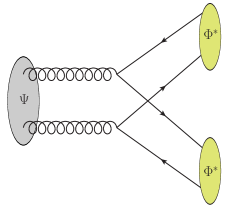
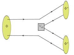
Figure 1: Fock-Tani amplitude is a mixture of a glueball decay into mesons (upper) and the meson decay (lower).

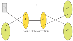
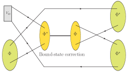
Figure 2: Fock-Tani bound-state correction amplitudes to the $q\bar{q}$ pair creation. There is no correction to the glueball amplitude.

III Numerical example

In our example we shall study the following decay channel $f_{0}(1500)\to 2\pi$. The amplitudes obtained are

$$h^{n\bar{n}}_{fi} = \gamma\,\left[b_{1}(p)\,e_{1}(p)-b_{2}(p)\,e_{2}(p)\right]\,Y_{00}$$

$$h^{s\bar{s}}_{fi} = 0$$

$$h^{g}_{fi} = \,\alpha_{s}\,b_{3}\,Y_{00}$$ (30)

where $Y_{00}$ is the spherical harmonic and

$$b_{1}(p) = \frac{32}{\pi^{1/4}}\sqrt{\frac{2}{3}}\beta_{q}^{5/2}\frac{3\beta_{\pi}^{2}(2\beta_{q}^{2}+\beta_{\pi}^{2})-(\beta_{q}^{2}+\beta_{\pi}^{2})\,p^{2}}{2\left(2{\beta_{q}}^{2}+{\beta_{\pi}}^{2}\right)^{7/2}}$$

$$b_{2}(p) = \frac{32}{\pi^{1/4}}\sqrt{\frac{2}{3}}\beta_{q}^{5/2}\frac{3\beta_{\pi}^{2}(4\beta_{q}^{2}+3\beta_{\pi}^{2})-4(\beta_{q}^{2}+\beta_{\pi}^{2})\,p^{2}}{3\left(4\beta_{q}^{2}+3\beta_{\pi}^{2}\right)^{7/2}}$$

$$b_{3} = \frac{4\sqrt{2}}{9\,\pi^{9/4}}\beta_{g}^{1/2}\,\beta_{\pi}^{2}\frac{(3\beta_{g}^{2}-2\beta_{\pi}^{2})}{(\beta_{g}^{2}+2\beta_{\pi}^{2})^{2}\,}\,\,$$

$$e_{1}(p) = \exp\left(-\frac{p^{2}}{8{\beta_{q}}^{2}+4{\beta_{\pi}}^{2}}\right)$$

$$e_{2}(p) = \exp\left(-\frac{\left(4{\beta_{q}}^{2}+5{\beta_{\pi}}^{2}\right){p}^{2}}{4{\beta_{\pi}}^{2}\left(4{\beta_{q}}^{2}+3{\beta_{\pi}}^{2}\right)}\right)$$ (31)

The second term in $h^{n\bar{n}}_{fi}$ is the bound-state correction for the light quark sector. If one sets $b_{2}(p)=0$, the bound state correction is turned off.

The $h_{fi}$ decay amplitude can be combined with a relativistic phase space to give the differential decay rate barnes

$$\frac{d\Gamma_{\alpha\rightarrow\beta\gamma}}{d\Omega}=2\pi\,\frac{PE_{\beta}E_{\gamma}}{M_{\alpha}}\,\,|h_{fi}|^{2}=2\pi\,\frac{PE_{\pi}^{2}}{M_{f_{0}}}\,\,|h_{fi}|^{2},$$ (32)

which after integration in the solid angle $\Omega$ gives rise to the decay rate, a usual choice for the meson momenta is made: $\vec{P}_{f_{0}}=0$ ($P=|\vec{P}_{\pi}|$). The experimental value for this decay channel is $\Gamma_{\rm exp}=38.04\,\pm{2.51}$ MeV pdg . The meson masses assumed in the numerical calculation have standard values of $M_{\pi}=138$ MeV and $M_{f_{0}}=1505$ MeV. There are two other sets of parameters, the first is the pair of coupling constants $\gamma$ and $\alpha_{s}$; the second are three wave-function widths $\beta_{\pi}$, $\beta_{q}$ and $\beta_{g}$. The value of $q\bar{q}$ coupling can be extracted from light meson, $\gamma=0.5$ barnes . The parameter $\alpha_{s}$ is the quark-gluon coupling, which is assumed to be fixed at the usual value $0.6$. The quark sector widths are in the range of 0.3 - 0.4 GeV barnes . For the pion, we shall fix $\beta_{\pi}=0.4$ GeV. The parameter $\beta_{q}$ is from the quark sector of $f_{0}(1500)$ and is chosen close, but slightly smaller than the pion’s value $\beta_{q}=0.3$ GeV. This leaves only one actually free parameter, the glueball’s width $\beta_{g}$, that should be adjusted. The best fit of $\Gamma$ to the range of the experimental value results in $\beta_{g}$ the order of 1.6 GeV. The mixing parameters $c_{i}$ used are from Ref. faessler where three models (A, B and C) are studied in detail. A comparison is shown in table (LABEL:tab1).

In conclusion, we have showed that the Fock-Tani formalism applied to meson decay with mixing is a promising approach and it exhibits bound-state corrections to the decay amplitude. This extends the OZI-allowed decays beyond the ordinary ${}^{3}P_{0}$ approach. Even though the choice of the microscopic Hamiltonians for the quark and gluon sectors is very simple, the essence of the procedure is clear and introduces a difference ranging from 7% to 11% in the decay rates. In future calculations an approach based on a Hamiltonian formulation, for example, QCD in the Coulomb gauge swanson1 ; swanson2 ; swanson3 , can replace some of the unknown parameters by fundamental quantities, extracted from QCD.

Table 1: Comparison of the decay rates in the ${}^{3}P_{0}$ and C${}^{3}P_{0}$ models

					$\Gamma$   (MeV)
Model	$c_{1}$	$c_{2}$	$c_{3}$	${}^{3}P_{0}$		C${}^{3}P_{0}$
A	0.43	-0.61	0.61	37.6		41.2
B	0.40	-0.90	0.19	19.8		22.3
C	0.31	-0.58	0.75	30.1		32.5

References

- (1) V. Mathieu, N. Kochelev and V. Vento, Int. J. Mod. Phys. E 18, 1 (2009).
- (2) V. Crede and C. A. Meyer, Prog in Part. and Nucl. Phys. 63, (2009) 74.
- (3) W. Ochs, J. Phys. G 40, 043001 (2013).
- (4) M. F. M. Lutz et al. [PANDA Collaboration], arXiv:0903.3905 [hep-ex].
- (5) G. S. Bali et al. [UKQCD Collaboration], Phys. Lett. B 309, 378 (1993).
- (6) H. Chen, J. Sexton, A. Vaccarino and D. Weingarten, Nucl. Phys. Proc. Suppl.34, 357 (1994).
- (7) C. J. Morningstar and M. J. Peardon, Phys. Rev. D 60, 034509 (1999).
- (8) A. Vaccarino and D. Weingarten, Phys. Rev. D 60, 114501 (1999).
- (9) M. Loan, X. Q. Luo and Z. H. Luo, Int. J. Mod. Phys. A 21, 2905 (2006).
- (10) Y. Chen et al., Phys. Rev. D 73, 014516 (2006).
- (11) E. Gregory, A. Irving, B. Lucini, C. McNeile, A. Rago, C. Richards and E. Rinaldi, JHEP 1210, 170 (2012).
- (12) H. Y. Cheng, C. K. Chua and K. F. Liu, Phys. Rev. D 92, no. 9, 094006 (2015).
- (13) C. Patrignani et al. [Particle Data Group], Chin. Phys. C 40 (2016) 100001 and 2017 update.
- (14) C. Amsler and F. E. Close, Phys. Lett. B 353, 385 (1995).
- (15) C. Amsler and F. E. Close, Phys. Rev. D 53, 295 (1996).
- (16) D. Weingarten, Nucl. Phys. B (Proc. Suppl) 53, 232 (1997).
- (17) M. Strohmiere-Preiek, T. Gutsche, R. Vinh Mau, A. Faessler, Phys. Rev. D 60, 054010 (1999).
- (18) F. E. Close, A. Kirk, Phys. Lett. B 483, 345 (2000).
- (19) F. E. Close, A. Kirk, Eur. Phys. J. C 21, 531 (2001).
- (20) F. E. Close, Q. Zhao, Phys. Rev. D 71, 094022 (2005).
- (21) M. L. L. da Silva and M. V. T. Machado, Phys. Rev. C 86, 015209 (2012).
- (22) M. V. T. Machado and M. L. L. da Silva, Phys. Rev. C 83, 014907 (2011).
- (23) A. H. Fariborz, A. Azizi and A. Asrar, Phys. Rev. D 91, 073013 (2015).
- (24) S. Janowski, D. Parganlija, F. Giacosa, and D. H. Rischke, Phys. Rev. D 84, 054007 (2011).
- (25) S. Janowski, F. Giacosa and D. H. Rischke, Phys. Rev. D 90, 114005 (2014).
- (26) F. Brüner, D. Parganlija and A. Robhan, Phys. Rev. D 91, 106002 (2015).
- (27) S. Dobbs, A. Tomaradze and K. K. Seth, Phys. Rev. D 91, 052006 (2015).
- (28) X. G. He and T. C. Yuan, Eur. Phys. J. C 75, 136 (2015).
- (29) M. Ablikim et al. (BES Collaboration), Phys. Lett. B 607, 243 (2005).
- (30) D. Hadjimichef, G. Krein, S. Szpigel and J. S. da Veiga, Phys. Lett. B 367, 317 (1996).
- (31) D. Hadjimichef, G. Krein, S. Szpigel and J. S. da Veiga, Ann. of Phys. 268, 105 (1998).
- (32) D.T. da Silva, M.L.L. da Silva, J.N. de Quadros, D. Hadjimichef, Phys. Rev. D 78, 076004 (2008).
- (33) M. L. L. da Silva, D. Hadjimichef, C. A. Z. Vasconcellos, B. E. J. Bodmann, J. Phys. G 32, 475 (2006).
- (34) E. S. Ackleh, T. Barnes and E. S. Swanson, Phys. Rev. D 54, 6811 (1996).
- (35) D. G. Robertson, E. S. Swanson, A. Szczepaniak, Chueng-Ryong Ji and S. R. Cotanch, Phys. Rev. D 59, 074019 (1999).
- (36) A. Szczepaniak, E. S. Swanson, Phys. Rev. D 62, 094027 (2000).
- (37) A. Szczepaniak, E. S. Swanson, Phys. Rev. D 65, 025012 (2001).